SFB/CPP-04-03
March 2004
Automated use of DIANA for two-fermion production at colliders

Abstract

We describe packages for the calculation of radiative corrections to two-fermion production at colliders. The packages use DIANA, and also QGRAF, FORM, Fortran, and further unix/linux tools. The one-loop calculations in the Standard Model are highly automatized with the package ai̊Talc. Further, the automatic determination of all the matrix elements for two-loop corrections to massive Bhabha scattering in QED and the classification of their topologies and prototypes is done with DIANA. A generalization to the Standard Model is straightforward.

1 INTRODUCTION

For the future $e^{+}e^{-}$ Linear Collider (LC) we need quite precise predictions of cross-sections for a variety of reactions, among them

$$e^{+}e^{-}\to{\bar{f}}f(\gamma),~{}~{}~{}~{}f=e,\mu,\tau,u,d,c,s,t,b.$$ (1)

The predictions have to be calculated with account of quantum corrections, typically with one- or two-loop accuracy. This has to be done in some model of field theory, notably the Standard Model or the Minimal Supersymmetric Standard Model. First complete one-loop calculations in the Standard Model for two-fermion production [1] and for Bhabha scattering [2] date back to 1979. After 25 years of perturbative calculations, the quest for a more or less complete automatization of this kind of calculation is natural. Nevertheless, only few packages for such a task are publicly available. We would like to mention CompHEP [3, 4, 5, 6, 7], FeynCalc/FeynArts/FormCalc/LoopTools/FF [8, 9, 10, 11], the grace project [12, 13] and SANC [14]. These packages have a variety of options to be used, but they do not go substantially beyond the one-loop level.

We are interested in a package for one- and two-loop calculations and we think that a prospective approach might be based on DIANA [15, 16, 17], an interface to QGRAF [18], to be combined also with FORM [19, 20] and Fortran, c++ and additional unix/linux tools.

Recently, we performed complete, high-precision one-loop calculations for (1) ($f\neq e$) in the Standard Model [21, 22] and demonstrated numerical agreements with the results of other groups, finally with up to eleven digits [23]. In a next step, the program package was completely rewritten in order to allow also the unexperienced user to create their own numerical code. The result is the package ai̊Talc. It covers also Bhabha scattering and will be described in more detail in the next section. In an earlier comparison for Bhabha scattering [24] a per mill agreement was established (see also [25, 26]). For realistic applications, one has to include also higher order corrections and to combine the so-called ‘weak library’ with a Monte Carlo code for the treatment of real bremsstrahlung; this is not discussed here. A dedicated comparison of this kind proved an accuracy of the order of $10^{-4}$ [27].

2 DIANA and two-fermion production

It is not so long ago that DIANA [28] was in a kind of experimental state. There exist several variants of the package with identical version numbers but with quite some different properties. For this reason, we decided to install a chain of versions with well-defined version properties at our location, presently the last one being v.2.35 [29]. From the user’s point of view, the package is characterized by a small number of input files:

• process.cnf – the file defines how to run DIANA; for examples see [29]; the incoming and outgoing particles plus loop order should be edited;

• Model.model – we have prepared four model files: QED.model, StandardModel0.model (a basic file with leptons

  only), StandardModel.model (complete with all masses and mixings), StandardModelC.model (with counter terms for neutral current $2f\to{2f}$, following [30], a typo corrected with [31]);

• FeynmanRules.frm – we have prepared three sets of Feynman rules: FeynmanRules0.frm (a simple version), FeynmanRules1.frm (with account of actual external momenta distribution), FeynmanRules2.frm (with account of internal momenta).

These files, together with a proper application of QGRAF and of additional DIANA options, give a huge flexibility to prepare a sample of prepared matrix elements of a given loop order in a given model for a subsequent FORM or MAPLE calculation. As an application in the Standard Model, the flavor non-diagonal reactions

$$e^{+}e^{-}\to{\bar{f}_{1}}f_{2},~{}~{}~{}~{}f_{1,2}=\mu,\tau,u,d,c,s,t,b$$ (2)

may also be treated. In this respect it would be extremely useful to have additional model files, e.g. for the minimal supersymmetric Standard Model. Some time ago, a project in XML was proposed, being intended on creating a standard for model files to be used in different CAS [32].

2.1 Full automatization of one-loop EWRC: ai̊Talc

A completely automated example, based on DIANA and other packages (see Fig. 1), is the project ai̊Talc [33], that provides also numerical output.

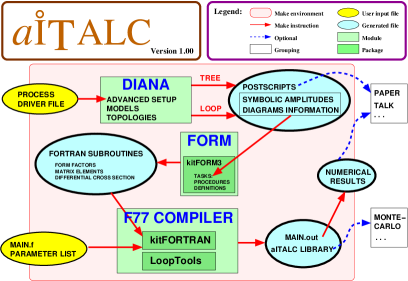
Figure 1: Flow chart of the ai̊Talc package.

It is designed to organize the calculation of tree-level and one-loop corrections to $2\rightarrow 2$ fermion processes, including Bhabha scattering (and in the near future also Moller scattering). This tool allows presently the calculation of unpolarized differential and integrated cross-sections. Differing from topfit [34], ai̊Talc treats all particle masses (including the electron mass) and mixings exactly, but does not cover hard photon emission.

In a simple driver file process.ini (simple form of process.cnf), the user specifies the ingoing and outgoing fermions. The determination of matrix elements, form factors and other kinematical routines proceeds then automatically. Later on, two Fortran files give access to the specific values of the parameters in our model and the numerical output of the code (i.e. a number of data points in the angular distribution, integrated cross section, running flags, etc).
Advanced features are not extremely user friendly, but still under development. Fermion masses are included by default, but may be neglected, and soft photonic corrections may be included (or not), as well as one may perform a full one-loop tensor integral reduction to the master integrals $A_{0}$, $B_{0}$, $C_{0}$ and $D_{0}$ in the Passarino-Veltman scheme [1]. All these possibilities will be described in more detail in a tutorial to be published soon.
Some more details may be found also in [23].

3 NUMERICAL ONE-LOOP RESULTS FOR BHABHA SCATTERING

The package ai̊Talc was used for a precise calculation of the one-loop electroweak corrections to fermion pair production and Bhabha scattering at LC energies. We compared the result of this with numerics from FeynArts/FormCalc/LoopTools [23].

The Table 1 shows an agreement of the two calculations of 14 digits for the $\mathcal{O}(\alpha)$ corrections (i.e. Born+QED+weak+soft) for the case with an exact treatment of $m_{e}\neq 0$, while the simplified comparison with $m_{e}\to 0$ does not provide more than 10 digits agreement. For practical purposes, this make no difference, of course.

Table 1: Cross-sections for $e^{-}e^{+}\to e^{-}e^{+}~{}(\gamma)$ at $\sqrt{s}=500~{}\mathrm{GeV}$ with a photon energy cut $E^{\mathrm{max}}_{\gamma_{\mathrm{soft}}}={\sqrt{s}}/{10}$.

$\begin{array}[]{rll}\hline\cr\cos{\theta}\phantom{\Big{|}}&{\left[\frac{\mathrm{d}\sigma}{\mathrm{d}\cos{\theta}}\right]}_{\mathcal{O}(\alpha^{3})}\quad\mathrm{(pb)}&\mathrm{Group}\\ \hline\cr-0.9&0.19344~{}50785~{}2686{\textsl{$3~{}6$}}\phantom{\cdot 10^{0}}&\textrm{{\sc{a}{\r{\i}}\raisebox{-1.4pt}{T}alc}{}}\\ -0.9&0.19344~{}50785~{}2686{\textsl{$2~{}2$}}\phantom{\cdot 10^{0}}&\textrm{FA/FC/LT}\\ \vspace{5pt}-0.9&0.19344~{}50785~{}{\textsl{$62637~{}9$}}\phantom{\cdot 10^{0}}&{\textsl{$m_{e}=0$}}\\ 0.0&0.54667~{}71794~{}6942{\textsl{$3~{}1$}}\phantom{\cdot 10^{0}}&\textrm{{\sc{a}{\r{\i}}\raisebox{-1.4pt}{T}alc}{}}\\ 0.0&0.54667~{}71794~{}6942{\textsl{$1~{}8$}}\phantom{\cdot 10^{0}}&\textrm{FA/FC/LT}\\ \vspace{5pt}0.0&0.54667~{}71794~{}{\textsl{$99961~{}4$}}\phantom{\cdot 10^{0}}&{\textsl{$m_{e}=0$}}\\ 0.9&0.17292~{}83490~{}6650{\textsl{$7~{}2$}}\cdot 10^{3}&\textrm{{\sc{a}{\r{\i}}\raisebox{-1.4pt}{T}alc}{}}\\ 0.9&0.17292~{}83490~{}6650{\textsl{$8~{}0$}}\cdot 10^{3}&\textrm{FA/FC/LT}\\ 0.9&0.17292~{}83490~{}6{\textsl{$1347~{}4$}}\cdot 10^{3}&{\textsl{$m_{e}=0$}}\\ \hline\cr\end{array}$

4 MASSIVE TWO-LOOP BHABHA SCATTERING

In a related activity, we use DIANA for a preparation of two-loop matrix elements in massive QED. We apply it for the solution of two different problems:

• The calculation of interferences of the two-loop amplitudes with the Born amplitudes (i.e. of the integrands for the determination of the scalar integrals);

• The determination of all prototypes.

Prototypes are topologies of diagrams, where additionally the different masses on internal lines are taken into account. An example is shown in Figure 2, where all prototypes with three external lines and six internal lines for the Bhabha process are given. Diagrams V1-V5 are genuine two loop QED vertices for the Bhabha process. Vertices V6-V10 come from extractions of one single line from two-loop QED box prototypes (altogether there are six genuine box prototypes). Strictly speaking, the prototypes V4-V6 and V8 should already be shrinked to five internal lines and classified into this class of prototypes because they have two internal lines with identical momentum. There are many more prototypes with five internal lines which come from the extraction of one (or two) lines of original vertex (or box) prototypes; we do not present them here. For these cases and for cases where even more lines are extracted, an automatization of the procedure for the identification of prototypes is very useful. Technically it has been made by merging information from DIANA and QGRAF in a subsequent FORM program.

Let us mention finally that out of all the prototypes shown in Figure 2 only V2 and V10 correspond to master integrals; all the others may be reduced to other master integrals. For a complete set of master integrals see [35].

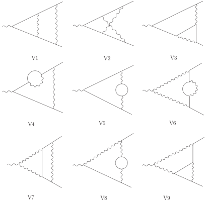
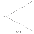
Figure 2: Vertices for the two-loop Bhabha process with six internal lines.

References

- [1] G. Passarino and M. Veltman, Nucl. Phys. B160 (1979) 151.
- [2] M. Consoli, Nucl. Phys. B160 (1979) 208.
- [3] E. Boos et al., MGU 89-63/140.
- [4] A. Pukhov et al., hep-ph/9908288.
- [5] E. Boos, for the CompHep collab., these proceedings.
- [6] A. Kryukov, for the CompHep collab., these proceedings.
- [7] A. Kryukov and L. Shamardin, these proceedings.
- [8] J. Küblbeck, M. Böhm and A. Denner, Comput. Phys. Commun. 60 (1990) 165.
- [9] T. Hahn, Comput. Phys. Commun. 140 (2001) 418, hep-ph/0012260.
- [10] T. Hahn and M. Pérez-Victoria, Comput. Phys. Commun. 118 (1999) 153, hep-ph/9807565.
- [11] G. van Oldenborgh, Comput. Phys. Commun. 66 (1991) 1.
- [12] G. Belanger et al., hep-ph/0308080.
- [13] J. Fujimoto et al., for the grace collab., these proceedings.
- [14] D. Bardin, P. Christova and L. Kalinovskaya, Nucl. Phys. Proc. Suppl. 116 (2003) 48.
- [15] M. Tentyukov and J. Fleischer, Comput. Phys. Commun. 132 (2000) 124, hep-ph/9904258.
- [16] M. Tentyukov and J. Fleischer, Nucl. Instrum. Meth. A502 (2003) 570.
- [17] J. Fleischer, A. Lorca and M. Tentyukov, these proceedings.
- [18] P. Nogueira, J. Comput. Phys. 105 (1993) 279.
- [19] J. Vermaseren, “Symbolic manipulation with FORM” (Computer Algebra Nederland, Amsterdam, 1991).
- [20] J.A.M. Vermaseren, (2000), math-ph/0010025.
- [21] J. Fleischer et al., Eur. Phys. J. C31 (2003) 37, hep-ph/0302259.
- [22] T. Hahn et al., hep-ph/0307132, LC-TH-2003-083.
-
[23]
A. Lorca,
http://www-zeuthen.desy.de/
~alorca/downloads/montpellier-11-03.pdf. - [24] D. Bardin, W. Hollik and T. Riemann, Z. Phys. C49 (1991) 485.
- [25] D. Bardin et al., Reports of the Working Group on Precision Calculations for the Resonance, report CERN 95–03 (1995), edited by D. Bardin, W. Hollik and G. Passarino, pp. 7–162, hep-ph/9709229.
- [26] Two Fermion Working Group, M. Kobel et al., hep-ph/0007180.
- [27] W. Beenakker and G. Passarino, Phys. Lett. B425 (1998) 199, hep-ph/9710376.
-
[28]
M. Tentyukov,
DIANA web page, http://
www.physik.uni-bielefeld.de/
~tentukov/diana.html . - [29] See the web page http://www-zeuthen.desy.de/theory/research/CAS.html .
- [30] A. Denner, Fortschr. Phys. 41 (1993) 307.
- [31] M. Böhm, H. Spiesberger and W. Hollik, Fortsch. Phys. 34 (1986) 687.
- [32] A. Demichev, A. Kryukov and A. Rodionov, hep-ph/0203102.
- [33] A. Lorca and T. Riemann, Zeuthen DIANA/aITALC project; the package ai̊Talc has been written by A. Lorca. See also the web page http://www-zeuthen.desy.de/theory/research/CAS.html .
- [34] J. Fleischer et al., Fortran program topfit.F v.0.92 (01 July 2003), http://www-zeuthen.desy.de/theory/num.html.
- [35] M. Czakon, J. Gluza and T. Riemann, hep-ph/0406203, to appear in Nucl. Phys. (Proc. Suppl.) B.