Cold Electroweak Baryogenesis

Abstract

We present arguments that the CKM CP-violation in the standard model may be sufficient for the generation of the baryon asymmetry, if the electroweak transition in the early universe was of the cold, tachyonic, type after electroweak-scale inflation. A model implementing this is described which complies with the CMB constraints and which is falsifiable with the LHC. Numerical simulations of the tachyonic transition with an effective CP-bias indicate that the observed baryon asymmetry can be generated this way.

1 Introduction

There are three families in the minimal Standard Model (SM), why? Such why-questions lie outside the scope of the model, but the thought ‘to allow for CP-violation and baryogenesis’ comes up easily. What is currently known experimentally about CP violation[1] can be attributed to the CKM matrix being complex, which is only possible for three or more families. This provides a strong motivation for finding a scenario for baryogenesis that makes use of this fact. SM electroweak baryogenesis[2], is believed by many to be impossible, because of ($i$) the weakness of CKM CP-violation, and ($ii$) the smoothness of the finite-temperature electroweak transition[3].

Of course, the SM assumes neutrinos to be massless, and a better framework is its extension that includes right-handed neutrino fields with renormalizable Yukawa couplings and a Majorana mass matrix, which may be called the Extended Standard Model (ESM). Leptogenesis is an attractive possibility within this framework[4]. However, it makes use of physics at the scale of $10^{10}$ GeV and it seems worth putting effort into scenarios closer to what we know on the scale $\lesssim 200$ GeV. So we must face issues ($i$) and ($ii$).

In the following a scenario[5, 6, 7, 8, 9] will be reviewed based on a cold (‘tachyonic’) electroweak transition caused by the coupling of a gauge-singlet inflaton to the ESM. First, we shall argue that CP violation is much stronger at zero temperature than often stated.

2 Magnitude of CKM CP-violation

The usual estimate for the magnitude of CP violation is[10, 2]

$$\delta_{\rm CP}=J\,(m_{u}^{2}-m_{c}^{2})(m_{c}^{2}-m_{t}^{2})(m_{t}^{2}-m_{u}^{2})(m_{d}^{2}-m_{s}^{2})(m_{s}^{2}-m_{b}^{2})(m_{b}^{2}-m_{d}^{2})/T^{12},$$ (1)

where $m_{u}$, …,$m_{b}$ are the quark masses and[1]

$$J=|{\rm Im}(V_{fg}V_{hi}V_{fi}^{*}V_{hg}^{*})|=(2.88\pm 0.33)\times 10^{-5}$$ (2)

is the simplest rephasing-invariant combination of the CKM matrix $V$. For $T=100$ GeV, of order of the finite-temperature electroweak phase transition, (1) gives the discouraging value $\delta_{\rm CP}\approx 10^{-19}$. At zero temperature one would replace $m_{j}/T$ by the Yukawa coupling $\lambda_{j}=\sqrt{2}\,m_{j}/v$, with $v=246$ GeV the vev of the Higgs field, giving

$$\delta_{\rm CP}=J\,(\lambda_{u}^{2}-\lambda_{c}^{2})(\lambda_{c}^{2}-\lambda_{t}^{2})(\lambda_{t}^{2}-\lambda_{u}^{2})(\lambda_{d}^{2}-\lambda_{s}^{2})(\lambda_{s}^{2}-\lambda_{b}^{2})(\lambda_{b}^{2}-\lambda_{d}^{2})\approx 10^{-22},$$ (3)

even smaller than (1). However, even with the Higgs field settled in its vev, the measured CP violating effects in accelerator experiments are at a much higher level than $10^{-23}$, e.g. the magnitude of the decay asymmetry $\epsilon^{\prime}$ in the $K^{0}-\bar{K}^{0}$ system is about[1] $4\times 10^{-6}$. This suggests that the above order of magnitude estimates of $\delta_{\rm CP}$ are misleading, at least at zero temperature.

To make the discussion more concrete, consider the effective action obtained by integrating our the fermions, $\Gamma_{\rm eff}=-\mbox{Tr}(\ln D)$, with $D$ the Dirac operator. In studies and discussions of electroweak baryogenesis, CP violation has been taken into account by approximating the CP asymmetry in $\Gamma_{\rm eff}$ by a leading dimension-six term[11]

$$-\mathcal{L}_{\rm CP}=\frac{3\delta_{\rm CP}}{16\pi^{2}M^{2}}\,\varphi^{\dagger}\varphi\;\mbox{tr}(F^{\mu\nu}\tilde{F}_{\mu\nu}),$$ (4)

where $F_{\mu\nu}$ is the SU(2) field strength tensor, $\tilde{F}_{\mu\nu}$ its dual, and $M$ is a mass depending on the scale of the problem. It could be the mass scale of an extension of the ESM. Within the ESM, at finite temperature, one could take $M=T$, but what to use when $T=0$? The fermion masses are $\propto\langle\varphi\rangle$, but $\varphi^{\dagger}\varphi/\langle\varphi^{\dagger}\varphi\rangle$ does not seem to make sense. The ordering of the terms in $\Gamma_{\rm eff}$ according to increasing dimension is questionable in a zero-temperature transition in which $\langle\varphi^{\dagger}\varphi\rangle$ increases from zero to some finite value.

Luckily, there exists a very detailed calculation of the zero-temperature effective action in a general chiral gauge model, based on a gauge-covariant derivative-expansion that is completely non-perturbative in the Higgs field, by L.L. Salcedo[12, 13]. We have applied his results to the ESM (without Majorana mass terms), and found that (4) is incorrect for this case: the rephasing invariant $J$ does not appear as a coefficient of $\mbox{tr}(F^{\mu\nu}\tilde{F}_{\mu\nu})$ times a function of the un-differentiated Higgs field[14]. The first CKM CP-violating contribution lies unfortunately still beyond the scope of Salcedo’s results, but a typical term is expected to have the form, in unitary gauge $A_{\mu}\to W_{\mu}$, $\varphi=(0,h)^{T}$,

$$\epsilon^{\kappa\lambda\mu\nu}W_{\kappa\lambda}^{a}W_{\mu\nu}^{b}W^{c}_{\rho}W^{d\rho}\,n^{\prime}_{abcd}(\lambda h),$$

where $a,b,c,d$ are $SU(2)$ indices and $n^{\prime}_{abcd}(\lambda h)$ is a non-trivial function of the Yukawa couplings times the Higgs field, $d_{j}\equiv\lambda_{j}\,h$. For e.g. $a=b=c=d=1$ the above expression violates CP and is expected to contain the invariant $J$. The crucial point is now that $n^{\prime}_{abcd}$ is expected to be a homogeneous function of the $d_{j}$. This is the case for the explicitly calculated coefficient functions at fourth order of the gauge-covariant derivative-expansion (involving four Lorentz indices), which are homogeneous of degree zero[12, 13], which is why (4) cannot occur. For the higher order term we expect that, when we rescale the Yukawa couplings $\lambda_{j}\to s\lambda_{j}$, the coefficient functions $n(\lambda h)$ scale by some negative power of $s$ (perhaps up to logarithms). This strongly suggests that we should not include the product of Yukawa couplings (3) in estimating $\delta_{\rm CP}$, leaving only $J$, which is a factor of about $10^{17}$ larger. For example,

$$\frac{(\lambda_{u}^{2}-\lambda_{c}^{2})(\lambda_{c}^{2}-\lambda_{t}^{2})(\lambda_{t}^{2}-\lambda_{u}^{2})(\lambda_{d}^{2}-\lambda_{s}^{2})(\lambda_{s}^{2}-\lambda_{b}^{2})(\lambda_{b}^{2}-\lambda_{d}^{2})}{(\lambda_{u}^{2}+\lambda_{c}^{2})(\lambda_{c}^{2}+\lambda_{t}^{2})(\lambda_{t}^{2}+\lambda_{u}^{2})(\lambda_{d}^{2}+\lambda_{s}^{2})(\lambda_{s}^{2}+\lambda_{b}^{2})(\lambda_{b}^{2}+\lambda_{d}^{2})}\simeq 0.99.$$

The argument applies only at zero temperature, since at finite $T$ a new scale appears, e.g. the thermal QCD quark mass $m_{\rm th}=g_{\rm s}T/\sqrt{6}$.

3 A falsifiable model of electroweak-scale inflation

Here we take seriously a minimal phenomenological extension of the ESM with an additional gauge-singlet inflaton that couples only to the Higgs field[9]. Its inflaton-Higgs potential is constructed after [7],

$$V(\sigma,\phi)=V_{0}-\frac{1}{p}\alpha_{p}\sigma^{p}+\frac{1}{q}\alpha_{q}\sigma^{q}-\frac{1}{2}\lambda_{\sigma\phi}\sigma^{2}\phi^{2}+\frac{1}{2}\mu_{\phi}^{2}\phi^{2}+\frac{1}{4}\lambda_{\phi}(\phi^{2})^{2},$$ (5)

where $\sigma$ is the inflaton field and $\phi^{2}\equiv 2\varphi^{\dagger}\varphi$. During inflation, $\sigma$ slow-rolls away from the origin. After inflation has ended it accelerates, and the effective Higgs mass

$$\mu_{\rm eff}^{2}=\mu_{\phi}^{2}-\lambda_{\sigma\phi}\sigma^{2}$$ (6)

changes sign from positive to negative, and the tachyonic electroweak transition starts. During the transition the baryon asymmetry is to be generated through the electroweak anomaly and the CKM CP-bias. To avoid sphaleron washout of the asymmetry the reheating temperature $T_{\rm rh}$ has to be small enough. Taking $V_{0}^{1/4}=100$ GeV, the Hubble rate is tiny, $H\approx 10^{-14}$ GeV, and $T_{\rm rh}=[30V_{0}/(\pi^{2}g_{*})]^{1/4}\simeq 51$ GeV ($g_{*}=86.25$ is the effective number of SM degrees of freedom below the $W$ mass), at which temperature the sphaleron rate is negligible.

As a phenomenological model it has to comply with what is currently known. Firstly, we have the CMB constraints[15]: the large-scale normalization $|\delta_{\bf k}|^{2}=(3.8\pm 0.5)\times 10^{-5}$, and the scalar spectral-index $n_{S}-1=-0.03\pm 0.03$. The latter is given by $n_{S}-1\simeq-(2/N)(p-1)/(p-2)$, with $N$ the number of e-folds before the end inflation, and $p>2$ for slow-roll to end naturally. For electroweak-scale inflation $N\simeq 24$, which is much lower than usually mentioned $\approx 60$, and the resulting $n_{S}-1\lesssim-0.083$ is too low. This is fixed[9] as mentioned below.

Secondly, in the minimum of the potential we have (approximating the cosmological constant by zero)

$$\frac{dV}{d\sigma}(v_{\sigma},v_{\phi}) = 0,\;\;\frac{dV}{d\phi}(v_{\sigma},v_{\phi})=0,\quad V(v_{\sigma},v_{\phi})=0,\quad v_{\phi}=246\;\mbox{GeV},$$

$$\mu_{\phi}^{2}-\lambda_{\sigma\phi}v_{\sigma}^{2} = -\frac{1}{2}\,m_{\phi}^{2},\;\;m_{\phi}^{2}=2\lambda_{\phi}v_{\phi}^{2},$$ (7)

where $m_{\phi}$ would be the SM Higgs mass, were it not that $\lambda_{\sigma\phi}$ leads to a considerable inflaton-Higgs mixing, to be addressed shortly. For definiteness we continue with $V_{0}^{1/4}=100$ GeV, $\mu_{\phi}=100$ GeV, $m_{\phi}=200$ GeV, for which the Higgs self-coupling $\lambda_{\phi}=0.33$, and we expect a particle mass above the current lower bound of 114 GeV[1].

Thirdly, the transition has to be reasonably rapid to allow for successful baryogenesis, which leads[7, 9] to the constraint $\lambda_{\sigma\phi}\gtrsim 0.01$. Essentially this constraint now fixes $p=5$ (the choices for $V_{0}$, $\mu_{\phi}$ and $m_{\phi}$ are not critical in this respect). The basic reason is that for $p<5$ the potential goes down rather slowly, giving a large $\sigma$-vev $v_{\sigma}$ and consequently a too small $\lambda_{\sigma\phi}$ (cf. (7)), whereas for $p>5$ the result is a ridiculously large $\lambda_{\sigma\phi}$. So we end up with non-renormalizable couplings, and to keep the powers of $\sigma$ as low as possible we have chosen $q=6$.

Returning to the minimum of the potential, the inflaton-Higgs mixing follows from the mass matrix

$$\partial^{2}V/\partial(\sigma,\phi)_{v_{\sigma},v_{\phi}}\Rightarrow\mbox{$m_{1}=385$ GeV, $m_{2}=125$ GeV, $\xi=0.44$ },$$

where $\xi$ is the mixing angle. The model thus predicts (only) two scalar particles with couplings to the rest of the SM determined by the mixing.

The CMB scalar spectral-index can be accommodated by adding terms $-\frac{1}{2}\,\alpha_{2}\sigma^{2}+\frac{1}{3}\,\alpha_{3}\sigma^{3}-\frac{1}{4}\,\alpha_{4}\sigma^{4}$ to the potential that were artificially set to zero in (5). For example, still with $\alpha_{3}=0$ we found that we could fit $n_{S}$ easily, see figure 1.

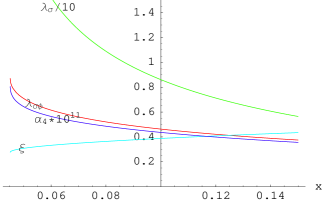
Figure 1: Dimension-full (left) and dimension-less (right) parameters as a function of $x\equiv\alpha_{2}m_{\rm Planck}^{2}/V_{0}$, for the central WMAP value $n_{S}-1=-0.03$.

Furthermore, in a one-loop study we verified that the potential can be kept flat enough so as not to upset slow-roll inflation; the non-renormalizable couplings lead to the conclusion that the model breaks down at scales around a TeV or so.

The flatness of the potential is finely tuned, but we stress that there is nothing wrong with this in a phenomenological model. It is a minimal extension of the SM that incorporates inflation as well as the tachyonic electroweak transition desired for baryogenesis, with signatures due to inflaton-Higgs mixing that allow it to be falsified by the LHC.

4 Tachyonic way-out-of-equilibrium transition

After inflation and before the transition, the universe is cold and approximately in the ground state corresponding to the symmetric phase of the SM. Then $\mu_{\rm eff}^{2}$ changes sign and the tachyonic transition develops. The initial part of such transitions with given ‘speed’ $\partial\mu_{\rm eff}^{2}/\partial t$ has been studied analytically as well as numerically[16, 17, 18, 19, 20]. We used the infinitely-fast quench,

$$\mu_{\rm eff}^{2} = +\mu^{2},\quad t<0$$

$$= -\mu^{2},\quad t>0,$$

in our simulations of the $SU(2)$-Higgs model described by

$$-\mathcal{L}=\frac{1}{2g^{2}}\,\mbox{tr}(F_{\mu\nu}F^{\mu\nu})+(D_{\mu}\varphi)^{\dagger}D^{\mu}\varphi+\mu_{\rm eff}^{2}\varphi^{\dagger}\varphi+\lambda(\varphi^{\dagger}\varphi)^{2}$$ (8)

as an explorative approximation for studying baryogenesis[8]. In the gaussian approximation the Fourier modes of a real component $\phi_{\bf k}$ of the Higgs field can be solved in the form $\alpha_{{\bf k}}\,e^{-i\omega_{k}^{-}t}+\beta_{\bf k}\,e^{i\omega_{k}^{-}t}$, with $\omega_{k}^{-}=\sqrt{-\mu^{2}+k^{2}}$. The modes with $k<\mu$ are unstable and grow exponentially $\propto e^{|\omega_{k}^{-}|t}$. After some time $\mu t\gg 1$, the equal-time correlators of $\phi_{\bf k}$ and $\pi_{\bf k}=\partial_{t}\phi_{\bf k}$ are generically well approximated by the classical distribution[21]

$$\exp\left[-\frac{1}{2}\sum_{|{\bf k}|<\mu}\left(\frac{|\xi^{+}_{\bf k}|^{2}}{n_{k}+1/2+\tilde{n}_{k}}+\frac{|\xi^{-}_{\bf k}|^{2}}{n_{k}+1/2-\tilde{n}_{k}}\right)\right],$$ (9)

where $\xi^{\pm}_{{\bf k}}=\frac{1}{\sqrt{2\omega_{k}}}\left(\omega_{k}\,\phi_{{\bf k}}\pm\pi_{\bf k}\right)$, and $n_{k}+1/2+\tilde{n}_{k}\gg 1$ and $n_{k}+1/2-\tilde{n}_{k}\ll 1$. So the typical $\xi_{k}^{+}$ grow large, while $\xi_{k}^{-}\to 0$; the distribution gets squeezed. In the classical approximation, realizations of the distribution (9) are used as initial conditions for time evolution using the classical equations of motion. For a weakly coupled system such as the SU(2)-Higgs sector of the SM we don’t have to wait till the occupation numbers have grown large, as the quantum and classical evolutions are identical in the gaussian approximation. Our ‘just a half’ initial conditions start directly at $t=0$, for which the occupation numbers $n_{k}=\tilde{n}_{k}=0$. In temporal gauge, $A_{0}=0$, the gauge field ${\bf A}$ is initialized to zero, and the initial $\partial_{t}{\bf A}$ is found from Gauss’ law[8].

In [22] we studied the particle-number distribution of the Higgs and W. For example, Fig. 2 shows how the W-particle $n_{k}$ in Coulomb gauge change in time. The rapid rise of the low momentum modes end at about $tm_{H}=7$ and after $tm_{H}=30$ the distribution does not change much anymore.

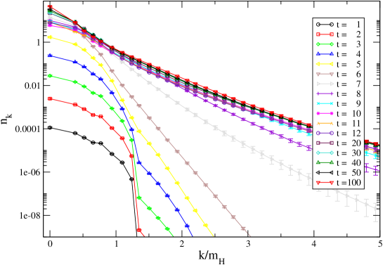
Figure 2: Coulomb-gauge W-particle numbers vs. momentum, time in units of $m_{H}^{-1}$.

These $n_{k}$ differ initially very much from the corresponding ones in the unitary gauge, but by time $tm_{H}=100$ they are practically the same. The particle numbers of the longitudinal polarization are initially similar to those of the Higgs but later appear to be slower in adjusting to the same distribution. The distributions at $tm_{H}=100$ can be fitted to Bose-Einstein distributions, separately in the more important low momentum region and for the higher momentum tails, giving effective temperatures and (at that time still considerable) chemical potentials. The overall lesson learned from these studies is that the transition is strongly out of equilibrium, and over after a few tens of $m_{H}^{-1}$. The finer details of thermalization will be different when the other d.o.f. from the quarks, gluons, etc. have been taken into account.

5 Baryogenesis

To estimate the asymmetry generated by the transition under influence of CP violation we simulated[8] the $SU(2)$-Higgs model with the effective CP violating term (4) added to the lagrangian (8). Although it was mentioned in section 2 that this term does not apply to the ESM, it is still interesting to see how large its parameter $\delta_{\rm CP}$ has to be in order to obtain the observed asymmetry. For the simulation we relabelled

$$\frac{3\delta_{\rm CP}}{16\pi^{2}M^{2}}\equiv\kappa,\quad k\equiv 16\pi^{2}m_{W}^{2}\,\kappa.$$ (10)

The baryon asymmetry is given by the anomaly equation

$$B(t)=3N_{\rm CS}(t)=3\frac{1}{16\pi^{2}}\int_{0}^{t}dt^{\prime}\int d^{3}x\,\left\langle\mbox{tr}\left(F_{\mu\nu}({\bf x},t^{\prime})\tilde{F}^{\mu\nu}({\bf x},t^{\prime})\right)\right\rangle,$$

where we assumed $B(0)=0$ (after inflation, just before the transition) and initial Chern-Simon number $N_{\rm CS}(0)=0$ (choice of gauge). Another useful observable is the winding number of the Higgs field,

$$N_{\rm w} = \frac{1}{24\pi^{2}}\int d^{3}x\,\epsilon_{klm}\mbox{tr}(\partial_{k}UU^{\dagger}\partial_{l}UU^{\dagger}\partial_{m}UU^{\dagger}),$$

$$U = \left(i\tau_{2}\varphi^{*},\,\varphi\right)/(\varphi^{\dagger}\varphi)^{1/2}\in SU(2).$$

At relatively low energy the gauge and Higgs fields are close to being pure-gauge and then $N_{\rm CS}(A)\approx N_{\rm w}(\varphi)$.

We simulated with parameters such that $m_{H}/m_{W}=1$ and $\sqrt{2}$, and various values of $k$ defined in (10). The initial conditions were ‘just a half’ (cf. Sect. 4) and ‘thermal’. The latter are simply Higgs-field realizations drawn from a free BE ensemble at low temperature $T=0.1\,m_{H}$, thermal noise that we used to get an impression of the sensitivity to the initial conditions. Figure 3 shows an example of how at first

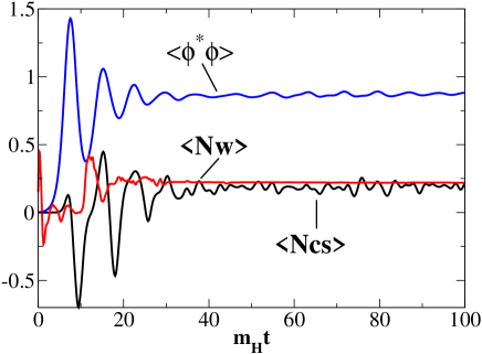
Figure 3: Averages: Higgs field $2\langle\varphi^{\dagger}\varphi\rangle/v^{2}$, Chern-Simons number $\langle N_{\rm CS}\rangle$ and Higgs winding number $\langle N_{\rm w}\rangle$, for $m_{H}=m_{w}$, $k=16$, ‘just a half’ initial conditions.

$\langle\varphi^{\dagger}\varphi\rangle$ rises exponentially and then settles into a damped oscillation near the vev. The Chern-Simons number has a small bump near $tm_{H}=7$, which we can understand analytically, after which it appears to resonate with $\langle\varphi^{\dagger}\varphi\rangle$ and settle near the winding number. The latter is at first erratic but then appears to stabilize earlier than $N_{\rm CS}$.

Fig. 4 shows results for the Chern-Simons number-density at time $tm_{H}=100$. There is no evidence for a sensitive dependence on the initial ensemble, and apparently the dependence on the magnitude of CP violation becomes non-linear for $k\gtrsim 5-10$. The dependence on the mass ratio $m_{H}/m_{W}$ appears limited. This is in contrast to what we found[21] in the 1+1D abelian-Higgs toy model, for which there is a sensitive dependence on $m_{H}/m_{W}$; it also showed nice linear behavior in the 1+1D analog $\kappa$ for small enough values.

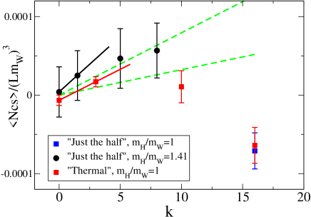
Figure 4: Chern-Simons number density vs. $k$.

The dashed lines are linear fits through the origin, ignoring the data at $k=0$ and 16. The straight full lines go through the two data points with lowest $k$. Including the data at $k=0$ is meaningful because these were generated with the same sequence of pseudo-random numbers as for $k=3$ ($m_{H}=m_{W}$) and $k=1.5$ ($m_{H}=\sqrt{2}\,m_{W}$). (Note that the $k=0$ data is shifted somewhat away from zero for $m_{H}=m_{W}$). Using the dashed-line fit for the case $m_{H}=\sqrt{2}\,m_{W}\simeq 114$ GeV gives a baryon asymmetry

$$\frac{n_{B}}{n_{\gamma}}=(0.46\pm 0.21)\times 10^{-2}\kappa\,m_{W}^{2}.$$

To fit the observed $n_{B}/n_{\gamma}\simeq 6.5\times 10^{-10}$, requires $\kappa$ to be

$$\kappa\approx\frac{1.4\times 10^{-7}}{m_{W}^{2}}\approx\frac{2.2\times 10^{-5}}{1{\rm TeV}^{2}}.$$

The 1 TeV scale is reasonable if we interpret $\mathcal{L}_{\rm CP}$ as being due to physics beyond the ESM. On the other hand, if we boldly assume that the results make sense for the ESM by taking the scale $M=m_{W}$, then the required $\delta_{\rm CP}$ turns out to be of the order of $J$ in (2):

$$\delta_{\rm CP}\approx 0.7\times 10^{-5}.$$

We consider this as very encouraging for further developing the scenario of cold electroweak baryogenesis.

References

- [1] S. Eidelman et al. [Particle Data Group Collaboration], Phys. Lett. B 592 (2004) 1.
- [2] V. A. Rubakov and M. E. Shaposhnikov, Usp. Fiz. Nauk 166, 493 (1996) [Phys. Usp. 39, 461 (1996)] [arXiv:hep-ph/9603208].
- [3] K. Kajantie, M. Laine, K. Rummukainen and M. E. Shaposhnikov, Nucl. Phys. B 466 (1996) 189 [arXiv:hep-lat/9510020].
- [4] M. Plümacher, these proceedings.
- [5] J. García-Bellido, D. Y. Grigoriev, A. Kusenko and M. E. Shaposhnikov, Phys. Rev. D 60, 123504 (1999) [arXiv:hep-ph/9902449].
- [6] L.M. Krauss and M. Trodden, Phys. Rev. Lett. 83, 1502 (1999).
- [7] E. J. Copeland, D. Lyth, A. Rajantie and M. Trodden, Phys. Rev. D 64, 043506 (2001) [arXiv:hep-ph/0103231].
- [8] A. Tranberg and J. Smit, JHEP 0311, 016 (2003) [arXiv:hep-ph/0310342].
- [9] B. van Tent, J. Smit and A. Tranberg, JCAP 0407, 003 (2004).
- [10] C. Jarlskog, Phys. Rev. Lett. 55, 1039 (1985).
- [11] M. E. Shaposhnikov, Nucl. Phys. B 287, 757 (1987).
- [12] L. L. Salcedo, Eur. Phys. J. C 20, 147 (2001) [arXiv:hep-th/0012166].
- [13] L. L. Salcedo, Eur. Phys. J. C 20, 161 (2001) [arXiv:hep-th/0012174].
- [14] J. Smit, arXiv:hep-ph/0407161.
- [15] D. N. Spergel et al., Astrophys. J. Suppl. 148, 175 (2003).
- [16] T. Asaka, W. Buchmuller and L. Covi, Phys. Lett. B 510, 271 (2001).
- [17] E. J. Copeland, S. Pascoli and A. Rajantie, Phys. Rev. D 65, 103517 (2002).
- [18] J. García-Bellido, M. García-Pérez, A. Gonzáles-Arroyo, Phys. Rev. D 67, 103501 (2003) [arXiv:hep-ph/0208228].
- [19] J. García-Bellido, M. García-Pérez, A. Gonzáles-Arroyo, Phys. Rev. D 69, 023504 (2004) [arXiv:hep-ph/0304285].
- [20] S. Borsanyi, A. Patkos and D. Sexty, Phys. Rev. D 68, 063512 (2003).
- [21] J. Smit and A. Tranberg, JHEP 0212, 020 (2002) [arXiv:hep-ph/0211243].
- [22] J. I. Skullerud, J. Smit and A. Tranberg, JHEP 0308, 045 (2003).
- [23] A. Tranberg, these proceedings.