Quark-Gluon Plasma Thermalization and Plasma Instabilities

Abstract

In this talk, I review the important role played by plasma instabilities in the thermalization of quark-gluon plasmas at very high energy. [Conference talk presented at Strong and Electroweak Mattter 2004, Helsinki, Finland, June 16–19.]

1 Introduction

Here is a basic question: What is the (local) thermalization time for quark-gluon plasmas (QGPs) in heavy ion collisions? That’s a difficult question, so let’s ask a simpler one: What is it for arbitrarily high energy collisions, where the running coupling constant is small, $\alpha_{\rm s}\ll 1$? Even that turns out to be complicated, so let me focus on an even simpler version, first posed by Baier, Mueller, Schiff and Son:[1] How does that time depend on $\alpha_{\rm s}$? In particular, in the saturation picture of heavy-ion collisions, what is the exponent $n$ in the relation

$$t_{\rm eq}\sim\frac{\alpha_{\rm s}^{n}}{Q_{\rm s}}\,?$$ (1)

Before discussing this question in more detail, I wish to make a general side comment about plasma physics. Plasma physics is complicated! This is made abundantly clear simply by looking at pictures of various plasma phenomena, such as the image in Fig. 1 of a solar coronal filament from NASA’s TRACE satellite. Theoretical discussions of quark-gluon plasmas, however, are generally much less complicated. There are several reasons why such discussions can usually avoid the full complication of traditional plasma physics. First, much of the theoretical literature discusses QGPs that are at or very close to thermal equilibrium. The physics of plasmas near global thermal equilibrium is much less complicated than the physics of non-equilibrium situations. Because electromagnetic interactions are long-ranged, traditional electromagnetic plasmas can be very complicated even when they are in local thermal equilibrium. Macroscopic currents in one region of the plasma can interact magnetically with other currents in other regions, over tremendous distance scales, creating complicated structures like Fig. 1. Non-Abelian plasmas, however, are somewhat different. From theoretical studies of the equilibrium properties of such plasmas, we know that the non-Abelian interactions cause magnetic confinement over distances of order $1/(g^{2}T)$. It is reasonable to assume that, even dynamically, color magnetic fields cannot exists on distance scales larger than the confinement length. So, unlike traditional electromagnetic plasmas, there are no large-distance magnetic fields. As far as the color degrees of freedom are concerned, the long-distance effective theory of a non-Abelian plasma is hydrodynamics rather than magneto-hydrodynamics.

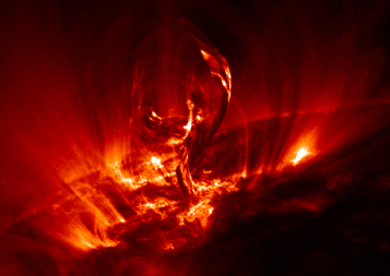
Figure 1: Image of a solar coronal filament from NASA’s TRACE satellite, from $\langle$http://antwrp.gsfc.nasa.gov/apod/ap000809.html$\rangle$.

The color magnetic fields can play a role on small scales. But the full complications of plasma physics might be ignored on small distance scales if the relevant physics on those scales is weakly interacting. This was the proposal of the original bottom-up scenario for thermalization of quark-gluon plasmas.[1] However, as we shall discuss, even at small distance scales, there can be plasma instabilities. These instabilities cause the growth of non-perturbatively large magnetic fields, bringing in some of the complicated non-linear physics of traditional plasma physics.

In the original bottom-up thermalization scenario of Baier et al., the starting assumption is the saturation scenario, which assumes that the formation of the quark-gluon plasma starts at times $t\sim Q_{\rm s}^{-1}$ dominated by gluons with momenta $p\sim Q_{\rm s}$, where the scale $Q_{\rm s}$ is known as the saturation scale. In this talk, these gluons will be referred to as “hard” gluons, since we will soon be discussing even softer momentum scales. This situation is depicted in Fig. 2a. The occupation numbers of each gluon mode are initially non-perturbative, with $f({\bm{x}},{\bm{p}})\sim 1/\alpha_{\rm s}$, where $f$ is the phase-space density. As the system expands 1-dimensionally immediately after the collision, the density per unit volume decreases, and one might therefore expect the hard gluon interactions to become more perturbative. To understand what happens next, let’s ignore these perturbative interactions for the moment and think about free expansion. As the nuclear pancakes fly apart after the collision, the gluons, which started in the center, will separate themselves in space according to the $z$ components of their velocities, as $\Delta z\sim v_{z}t$. This is depicted in Fig. 2b. The gluons left in the central region will be those with small $v_{z}$, as shown in Fig. 2c. As a result, the momentum distribution in that central region will have an anisotropic pancake shape, as shown in Fig. 2d. In other regions, the momentum distribution is simply a boosted version of this—that is, it looks the same if one works in the local rest frame.

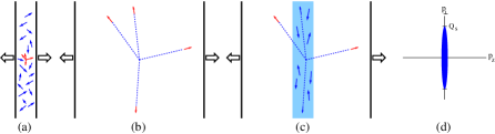
Figure 2: Approximately free expansion at relatively early stages of the bottom-up scenario.

It should be emphasized that this anisotropic momentum distribution has nothing to do with the usual elliptic flow distribution measured in non-central heavy ion collisions. Fig. 2d is a statement of the local momentum distribution in the local fluid rest frame at very early times, before collisions have brought the system to local equilibrium. Elliptic flow is instead a measure of the net fluid flow on large scales of a system that has quite possibly come to local thermal equilibrium (and so locally has isotropic momentum distributions in the local fluid rest frame).

In the original bottom-up scenario, equilibration of the plasma was assumed to occur through individual 2-body collisions between particles (with some LPM effect thrown in). In the first stage of the scenario, $1\ll Q_{\rm s}t\ll\alpha^{-5/2}$, the important processes were small angle scattering, which slightly widens the hard particle distribution in $p_{z}$, and soft Bremsstrahlung from colliding hard particles, which creates soft gluons with momenta $k\ll Q_{\rm s}$. In the second stage, $\alpha^{-5/2}\ll Q_{\rm s}t\ll\alpha^{-13/5}$, these soft gluons come to dominate the number density of particles, but the hard gluons still dominate the energy density. Collisions between the soft gluons cause the soft gluons to thermalize. Finally, the hard particles begin to lose energy by Bremsstrahlung plus cascading, as shown in Fig. 3. In this scenario, local thermalization became complete at $Q_{\rm s}t\sim\alpha^{-13/5}$.

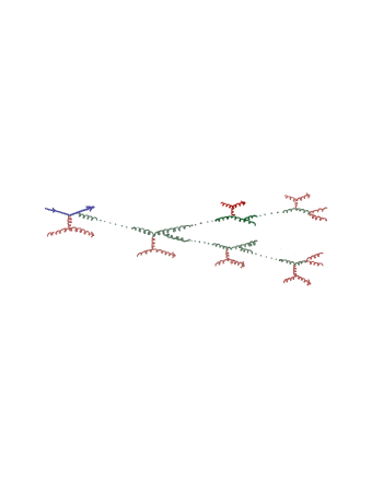
Figure 3: Cascading process for energy transfer from hard particles to soft sector in the original bottom-up scenario. Straight lines denote hard gluons, $p\sim Q_{\rm s}$.

The original bottom-up scenario overlooked the possibility that collective processes (as opposed to sequences of individual collisions) could play an important role in the equilibration of the plasma. In the case at hand, these collective processes are related to the appearance of plasma instabilities in the analysis of the equilibration of the quark-gluon plasma.

2 Plasma Instabilities

The hero of this story is Stan Mrówczyński,[2, 3, 4] who over the years has been the major proponent of the idea that plasma instabilities are important for the equilibration of the quark-gluon plasma. The application of this idea to bottom-up thermalization was made by myself, Jonathan Lenaghan and Guy Moore.[5] A selection of other folks who have considered the idea past and present include Refs. heinz_conf–birse and the work by Romatschke and Strickland,[10] which was reported on at this conference.

Let me start with a slightly formal explanation of the origin of plasma instabilities, and I will give a more physical picture afterward. Imagine calculating the self-energy $\Pi(\omega,k)$ for a particle moving through the plasma. The self-energy represents the effect on the particle of forward-scattering off of other particles in the medium, as in Fig. 4a, which one can alternatively calculate as in Fig. 4b using one’s favorite formalism for field theory in a medium, or more simply calculate using linearized kinetic theory. (Here, the straight lines represent hard particles, which are gluons in the bottom-up scenario.) The result is the same either way. Generically, if the momentum distribution $f({\bm{p}})$ of hard particles is anisotropic, one finds that there are negative eigenvalues of $\Pi^{ij}(0,{\bm{k}})$. (See, for example, the general arguments in Ref. alm.) Such negative eigenvalues indicate instabilities at small $k$, which means exponentially growing soft gauge fields.

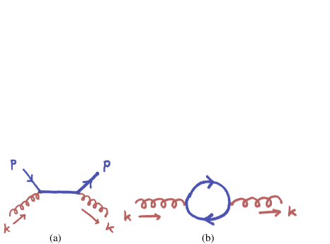
Figure 4: Self-energy of soft modes due to hard particles.

Let me give an analogy from scalar $\phi^{4}$ theory at finite temperature. Imagine integrating out the hard particles to get an effective thermal self-energy $\Pi$ of order $\lambda T^{2}$. The effective linearized equation of motion is then

$$\omega^{2}\phi=(k^{2}+m_{0}^{2}+\Pi)\phi\equiv(k^{2}+m_{\rm eff}^{2})\phi.$$ (2)

Let’s set $m_{0}=0$ to improve the analogy, since gluons do not have any intrinsic mass. If we were in a situation where $k^{2}+\Pi$ were less than zero, then there would be solutions with $\omega=\pm i\Gamma$ pure imaginary, which would lead to exponentially growing solutions to the linearized equation. Alternatively, think about the effective potential,

$$V_{\rm eff}(\phi)=m_{\rm eff}^{2}\phi^{2}+\lambda\phi^{4}=\Pi\phi^{2}+\lambda\phi^{4}.$$ (3)

If $\Pi<0$, as happens in some multi-scalar theories,[11] then the potential looks like a double-well potential: the naive vacuum $\phi=0$ is unstable; there is exponential growth from $\phi=0$ of modes with $k<(-\Pi)^{1/2}$; and the growth stops once $\phi$ becomes non-perturbatively large.

Now let’s turn to a physical picture of the instability, which I will adapt from Refs. mrow,alm. For simplicity, imagine two inter-penetrating, homogeneous streams of charged hard particles, one going up the page and one going down, which I’ll call the $\pm x$ directions. Now also imagine that, due to some fluctuation, there is a very tiny seed magnetic field of the form ${\bm{B}}=B{\bm{e}}_{y}\cos(kz)$, as shown in Fig. 5a. Here, crosses denote magnetic fields pointing into the page, and dots fields pointing out of the page. Using the right-hand rule, you can check that the magnetic fields bend the trajectories of positively charged particles in the directions shown. This then focuses the net downward and upward currents into different channels, as shown in Fig. 5b. Again using the right-hand rule, one finds that these currents in turn create magnetic fields that add to the original seed field. With bigger fields, the effect becomes more pronounced, and the fields continue to grow through this mechanism. This is the Weibel instability.

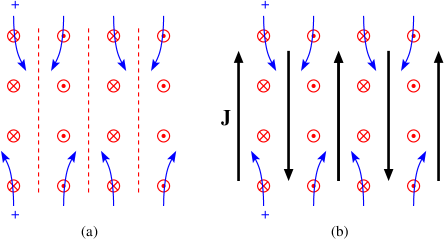
Figure 5: Origin of Weibel instability.

We get a seemingly contradictory picture of what happens if we considers hard particles which move in other directions, such as in Fig. 6. Following how these particles are by the seed magnetic field, we find they are directed a little more upward in some regions and a little more downward in others. This results in a net current as shown in the picture, but these currents create magnetic fields which oppose the seed field. Let ${\bm{p}}$ be the original momentum of the hard particle and ${\bm{k}}$ the wave number of the soft magnetic field fluctuation. What happens is that particles with ${\bm{p}}\cdot{\bm{k}}\simeq 0$ get trapped in valleys, as shown in Fig. 6b, and give the de-stabilizing effect discussed earlier. Other particles, with ${\bm{p}}\cdot{\bm{k}}\not\simeq 0$, are “untrapped” as in Fig. 6a, and give a stabilizing effect. For isotropic $f({\bm{p}})$, these two contributions turn out to cancel, giving $\Pi^{ij}(0,{\bm{k}})=0$.

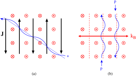
Figure 6: (a) untrapped particles; (b) trapped particles.

Now, instead of an isotropic hard particle distribution $f({\bm{p}})$, think of the one depicted earlier in Fig. 2d. For ${\bm{k}}$ in the $z$ direction, we will get a relatively smaller percentage of particles with ${\bm{p}}\cdot{\bm{k}}\simeq 0$ than we would with an isotropic distribution, and so the net effect will be stabilizing. On the other hand, for ${\bm{k}}$ in the $\perp$ direction, we will get a relatively larger percentage of particles with ${\bm{p}}\cdot{\bm{k}}\simeq 0$ than we would with an isotropic distribution, and so the net effect will be de-stabilizing. For ${\bm{k}}$ at significant angles to the axis, most of the particles with have ${\bm{p}}\cdot{\bm{k}}\not\simeq 0$, and we will tend to get stability. The moral of this story, to which we will later return, is that the unstable modes associated with this distribution have ${\bm{k}}$ pointing very close to the $z$ axis.

3 When does the growth stop?

As in the scalar analogy discussed earlier, the growth of instabilities should stop when the soft fields become non-perturbatively large. From considering covariant derivatives $D=\partial-igA$, the effects of soft fields $A$ become non-perturbative when $A\sim\partial/g$. There are two possibilities for the momentum scale associated with the derivatice $\partial$. The first, a possibility for both QCD and QED, is that growth stops when the effects of the soft fields on hard particles becomes non-perturbative, which will happen when $A\sim p_{\rm hard}/g$ and corresponds to the trajectories of hard particles being bent dramatically from straight lines. The second possibility, which cannot occur in QED, is that growth stops when the non-Abelian self-interactions of the soft fields become non-perturbative. This corresponds to $A\sim k_{\rm soft}/g$. Whenever there is a significant separation $k\ll p$ between soft and hard physics (as in the bottom-up scenario), these two possibilities correspond to parametrically different scales for $A$.

Jonathan Lenaghan and I conjecture[12] that growing QCD instabilities “abelianize.” That is, the growth stops when $A\sim k_{\rm soft}/g\sim|\Pi|^{1/2}/g$, just as in QED. That in turn suggests that the complicated stuff that happens afterward is closely related to the mainstream plasma physics of (collisionless) relativistic QED plasmas. What follows is a summary of suggestive arguments that we make for abelianization.

Start with the general HTL effective action for anisotropic $f({\bm{p}})$, which I adapt from Mrówczyński, Rebhan, and Strickland.[13] Shcematically,

$$S_{\rm eff}=-\int_{x}F^{2}-g^{2}\int_{x{\bm{p}}}f({\bm{p}})\,W^{2},$$ (4)

$$W\equiv W_{\alpha}(x,{\bm{p}})\equiv\frac{p^{\mu}}{p\cdot D}\,F_{\mu\alpha}.$$ (5)

Now imagine finding the effective potential $V_{\rm eff}$ by looking at $S_{\rm eff}$ for time-independent configurations in $A_{0}{=}0$ gauge. There is a problem, which is that $(p\cdot D)^{-1}$ is a complicated, non-local operator. But now recall that, for the hard particle distribution of Fig. 2d, the typical unstable modes have ${\bm{k}}$ pointing very close the $z$ direction. Inspired by this, let’s ignore $k_{\perp}$ altogether and consider configurations ${\bm{A}}={\bm{A}}(z)$ depending on $z$ only. There is then an amazing simplification, noted by Blaizot and Iancu:[14] $W$ given by (5) then turns out to be linear in $A$. As a result, the HTL term $g^{2}\int fW^{2}$ in the effective action (4) is then quadratic in $A$. That means that it consists of nothing but the HTL self-energy, so that

$$S_{\rm eff}[{\bm{A}}(z)]=-\int_{x}F^{2}-\int_{x}A\Pi A.$$ (6)

The $\Pi$ here is for ${\bm{k}}$’s proportional to $\hat{z}$. It is also transverse, corresponding to $\Pi_{\perp}(0,k\hat{z})$. This turns out not to depend on the magnitude $k$ of ${\bm{k}}$. I will define the constant $-\mu^{2}\equiv\Pi_{\perp}(0,k\hat{z})$. The effective potential from (6) is then

$$V_{\rm eff}[A(z)]=B^{2}-\mu^{2}A_{\perp}^{2},$$ (7)

where $B$ is the full, non-Abelian magnetic field, which includes non-linear terms in $A$. Now consider the arbitrarily soft limit $k\to 0$, where the derivative term in $B$ vanishes and only the non-Abelian commutator term survives:

$$V_{\rm eff}\to[A_{x},A_{y}]^{2}-\mu^{2}(A_{x}^{2}+A_{y}^{2}).$$ (8)

What does this potential look like? As an example, let’s consider just two of the degrees of freedom: color 1 of $A_{x}$ and color 2 of $A_{y}$. A plot of the resulting potential is shown in Fig. 7. As one moves away from $A=0$, the potential bends down due to the $-\mu^{2}A^{2}$ term. If both colors are present, it then later bends back up again due to the quartic $[A_{x},A_{y}]^{2}$ term. However, if the configuration is single-colored ($A_{x}^{(1)}=0$ or $A_{y}^{(2)}=0$), the commutator vanishes, and the potential continues to run away. If we were to roll a ball from the origin in such a potential, it would eventually roll away down into one of the Abelian directions $[A_{x},A_{y}]=-0$.

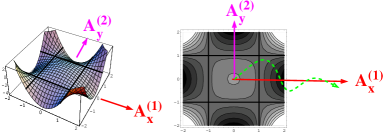
Figure 7: A picture of the effective potential.

The above argument suggests the following conjecture, which is the conclusion of my talk: The growth of Weibel instabilities eventually “abelianizes” the soft gauge fields into the maximal Abelian subgroup of the gauge group. For SU(2) gauge theory, this would give traditional U(1) plasma physics. For SU(3) gauge theory, it would give U(1)$\times$U(1) plasma physics, corresponding to two copies of Abelian electromagnetism. Further discussion, including corroboration from numerical simulation results of a related toy model, may be found in Ref. al.

References

- [1] R. Baier, A. H. Mueller, D. Schiff and D. T. Son, Phys. Lett. B502, 51 (2001) [hep-ph/0009237].
- [2] S. Mrówczyński, Phys. Lett. B214, 587 (1988); ibid. B314, 118 (1993); Phys. Rev. C49, 2191 (1994); Phys. Lett. B393, 26 (1997) [hep-ph/9606442].
- [3] S. Mrówczyński and M. H. Thoma, Phys. Rev. D62, 036011 (2000) [hep-ph/0001164].
- [4] J. Randrup and S. Mrówczyński, Phys. Rev. C68, 034909 (2003) [nucl-th/0303021].
- [5] P. Arnold, J. Lenaghan and G. D. Moore, JHEP 0308, 002 (2003) [hep-ph/0307325].
- [6] U. W. Heinz, Nucl. Phys. A418, 603C (1984).
- [7] Y. E. Pokrovsky and A. V. Selikhov, JETP Lett. 47, 12 (1988) [Pisma Zh. Eksp. Teor. Fiz. 47, 11 (1988)]; Sov. J. Nucl. Phys. 52, 146 (1990) [Yad. Fiz. 52, 229 (1990)]. ibid. 52, 385 (1990) [Yad. Fiz. 52, 605 (1990)].
- [8] O. P. Pavlenko, Sov. J. Nucl. Phys. 55, 1243 (1992) [Yad. Fiz. 55, 2239 (1992)].
- [9] M. C. Birse, C. W. Kao and G. C. Nayak, Phys. Lett. B570, 171 (2003) hep-ph/0304209.
- [10] P. Romatschke and M. Strickland, Phys. Rev. D68, 036004 (2003) [hep-ph/0304092].
- [11] S. Weinberg, Phys. Rev. D9, 3357 (1974).
- [12] P. Arnold and J. Lenaghan, hep-ph/0408052.
- [13] S. Mrowczynski, A. Rebhan and M. Strickland, Phys. Rev. D70, 025004 (2004) [hep-ph/0403256].
- [14] J. P. Blaizot and E. Iancu, Phys. Lett. B326, 138 (1994) [hep-ph/9401323].