Prethermalisation and
the build-up of the Higgs effect

D. SEXTY and A. PATKÓS111Work supported by grant T-037689 of the Hungarian National Science Foundation. Department of Atomic Physics
Eötvös University
H-1117 Pázmány Péter sétány 1/A
E-mail: denes@achilles.elte.hu, patkos@ludens.elte.hu
Abstract

Real time field excitations in the broken symmetry phase of the classical abelian Gauge+Higgs model are studied numerically in the unitary gauge, for systems starting from the unstable maximum of the Higgs potential.

1 Introduction

Tracking the transmutation of the angular component of a complex Higgs field into the longitudinal polarisation state of the gauge field during the termination of inflation in hybrid models might reveal interesting details of the real time Higgs effect and of the electroweak dynamics [1]. The excitation rate of the different polarisation states might be different as well as the thermal relaxation rates [2]. The production of gauged cosmic strings is another important aspect of this process[3]. Our numerical study concentrates on the non-equilibrium phase transition aspects.

2 Partial Pressures and Energy Densities of the Model

The main observables studied in the present investigation of the classical abelian Gauge+Higgs model,

L=14FμνFμν+12DμΦ(DμΦ)V(Φ),V(Φ)=12m2Φ2+λ24Φ4formulae-sequence𝐿14subscript𝐹𝜇𝜈superscript𝐹𝜇𝜈12subscript𝐷𝜇Φsuperscriptsuperscript𝐷𝜇Φ𝑉Φ𝑉Φ12superscript𝑚2superscriptΦ2𝜆24superscriptΦ4L=-\frac{1}{4}F_{\mu\nu}F^{\mu\nu}+\frac{1}{2}D_{\mu}\Phi(D^{\mu}\Phi)^{*}-V(\Phi),\quad V(\Phi)=\frac{1}{2}m^{2}\Phi^{2}+\frac{\lambda}{24}\Phi^{4} (1)

are the partial energy densities and pressures:

ϵitalic-ϵ\displaystyle\epsilon =\displaystyle= ϵρ+ϵT+ϵL,p=pρ+pT+pL,subscriptitalic-ϵ𝜌subscriptitalic-ϵ𝑇subscriptitalic-ϵ𝐿𝑝subscript𝑝𝜌subscript𝑝𝑇subscript𝑝𝐿\displaystyle\epsilon_{\rho}+\epsilon_{T}+\epsilon_{L},\quad p=p_{\rho}+p_{T}+p_{L},
ϵρsubscriptitalic-ϵ𝜌\displaystyle\epsilon_{\rho} =\displaystyle= 12Πρ2+12(ρ)2+V(ρ),pρ=12Πρ216(ρ)2V(ρ),12superscriptsubscriptΠ𝜌212superscript𝜌2𝑉𝜌subscript𝑝𝜌12superscriptsubscriptΠ𝜌216superscript𝜌2𝑉𝜌\displaystyle\frac{1}{2}\Pi_{\rho}^{2}+\frac{1}{2}(\nabla\rho)^{2}+V(\rho),\quad p_{\rho}=\frac{1}{2}\Pi_{\rho}^{2}-\frac{1}{6}(\nabla\rho)^{2}-V(\rho),
ϵTsubscriptitalic-ϵ𝑇\displaystyle\epsilon_{T} =\displaystyle= 12[𝚷T2+(×𝐀T)2+e2ρ2𝐀T2],12delimited-[]superscriptsubscript𝚷𝑇2superscriptsubscript𝐀𝑇2superscript𝑒2superscript𝜌2superscriptsubscript𝐀𝑇2\displaystyle\frac{1}{2}[{\bf\Pi}_{T}^{2}+(\nabla\times{\bf A}_{T})^{2}+e^{2}\rho^{2}{\bf A}_{T}^{2}],
pTsubscript𝑝𝑇\displaystyle p_{T} =\displaystyle= 16[𝚷T2+(×𝐀T)2e2ρ2𝐀T2],16delimited-[]superscriptsubscript𝚷𝑇2superscriptsubscript𝐀𝑇2superscript𝑒2superscript𝜌2superscriptsubscript𝐀𝑇2\displaystyle\frac{1}{6}[{\bf\Pi}_{T}^{2}+(\nabla\times{\bf A}_{T})^{2}-e^{2}\rho^{2}{\bf A}_{T}^{2}],
ϵLsubscriptitalic-ϵ𝐿\displaystyle\epsilon_{L} =\displaystyle= 12[𝚷L2+e2ρ2(𝐀L2+1(e2ρ2)2(ΠL)2)],12delimited-[]superscriptsubscript𝚷𝐿2superscript𝑒2superscript𝜌2superscriptsubscript𝐀𝐿21superscriptsuperscript𝑒2superscript𝜌22superscriptsubscriptΠ𝐿2\displaystyle\frac{1}{2}\left[{\bf\Pi}_{L}^{2}+e^{2}\rho^{2}\left({\bf A}_{L}^{2}+\frac{1}{(e^{2}\rho^{2})^{2}}(\nabla\Pi_{L})^{2}\right)\right],
pLsubscript𝑝𝐿\displaystyle p_{L} =\displaystyle= 16[𝚷L2e2ρ2𝐀L2]+121e2ρ2(𝚷L)2.16delimited-[]superscriptsubscript𝚷𝐿2superscript𝑒2superscript𝜌2superscriptsubscript𝐀𝐿2121superscript𝑒2superscript𝜌2superscriptsubscript𝚷𝐿2\displaystyle\frac{1}{6}[{\bf\Pi}_{L}^{2}-e^{2}\rho^{2}{\bf A}_{L}^{2}]+\frac{1}{2}\frac{1}{e^{2}\rho^{2}}(\nabla{\bf\Pi}_{L})^{2}. (2)

Index T𝑇T refers to the transversal, L𝐿L to the longitudinal part of the gauge field 𝐀𝐀\bf A. The expressions are valid in the unitary gauge: ρ=|Φ|𝜌Φ\rho=|\Phi|. A0subscript𝐴0A_{0} was eliminated with the Gauss constraint. It was checked numerically that in equilibrium ϵρ:ϵL:ϵT=1:1:2:subscriptitalic-ϵ𝜌subscriptitalic-ϵ𝐿:subscriptitalic-ϵ𝑇1:1:2\epsilon_{\rho}:\epsilon_{L}:\epsilon_{T}=1:1:2 within statistical fluctuations [4].

The equations of motion derived from (1) were solved in the A0=0subscript𝐴00A_{0}=0 gauge and the solutions were transformed to the unitary gauge for measurements. Initially ρ(𝐱,t=0)=0𝜌𝐱𝑡00\rho({\bf x},t=0)=0 was put uniformly. Inhomogenuous modes beyond the region of spinodal instability (up to |𝐤|5|m|)|{\bf k}|\leq 5|m|) were filled with low amplitude white noise. The spatial lattice spacing was chosen to as=0.35|m|1subscript𝑎𝑠0.35superscript𝑚1a_{s}=0.35|m|^{-1} and the time step δt=0.04|m|1𝛿𝑡0.04superscript𝑚1\delta t=0.04|m|^{-1}.

3 Spectral Analysis of the Process of Excitation

Spectral representation of the energy densities ϵ(𝐤)italic-ϵ𝐤\epsilon({\bf k}) (pressures p(𝐤)𝑝𝐤p({\bf k})) were defined using the Fourier transform of the square root of various pieces of the local energy densities (pressures) and taking their absolute squares.

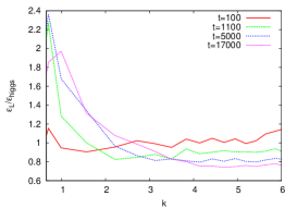
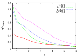
In Fig.1 the degrees of excitation ϵT(𝐤)/ϵρ(𝐤)subscriptitalic-ϵ𝑇𝐤subscriptitalic-ϵ𝜌𝐤\epsilon_{T}({\bf k})/\epsilon_{\rho}({\bf k}) and ϵL(𝐤)/ϵρ(𝐤)subscriptitalic-ϵ𝐿𝐤subscriptitalic-ϵ𝜌𝐤\epsilon_{L}({\bf k})/\epsilon_{\rho}({\bf k}) are displayed as functions of |𝐤|𝐤|{\bf k}| at different times. The low frequency part of ϵL(𝐤)subscriptitalic-ϵ𝐿𝐤\epsilon_{L}({\bf k}) develops an over-excited peak, while ϵT(𝐤)subscriptitalic-ϵ𝑇𝐤\epsilon_{T}({\bf k}) is excited weakly at early times. Their slow evolution towards equipartition defines an extremely long thermalisation time-scale (τ>105|m|1𝜏superscript105superscript𝑚1\tau>10^{5}|m|^{-1}).

Refer to caption Refer to caption

Figure 1: Evolution of the longitudinal (left) and transversal (right) energy excitations relative to the 𝐤0𝐤0{\bf k}\neq 0 Higgs modes.

4 Signals for Prethermalisation

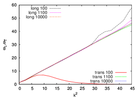
The dispersion relations ω2(𝐤)superscript𝜔2𝐤\omega^{2}({\bf k}) of the modes (ρ,𝐀T)𝜌subscript𝐀𝑇(\rho,{\bf A}_{T}) are obtained as |Πρ(𝐤)|2/|ρ(𝐤)|2superscriptsubscriptΠ𝜌𝐤2superscript𝜌𝐤2|\Pi_{\rho}({\bf k})|^{2}/|\rho({\bf k})|^{2} and |ΠT(𝐤)|2/|𝐀T(𝐤)|2superscriptsubscriptΠ𝑇𝐤2superscriptsubscript𝐀𝑇𝐤2|\Pi_{T}({\bf k})|^{2}/|{\bf A}_{T}({\bf k})|^{2}. For the longitudinal mode inspection of ϵLsubscriptitalic-ϵ𝐿\epsilon_{L} in (2) suggests ωL2(𝐤)|[e2ρ2𝐀L](𝐤)|2/|ΠL(𝐤)|2.superscriptsubscript𝜔𝐿2𝐤superscriptdelimited-[]superscript𝑒2superscript𝜌2subscript𝐀𝐿𝐤2superscriptsubscriptΠ𝐿𝐤2\omega_{L}^{2}({\bf k})\equiv|[e^{2}\rho^{2}{\bf A}_{L}]({\bf k})|^{2}/|\Pi_{L}({\bf k})|^{2}. The masses of the longitudinal and transversal modes become degenerate early when calculated from modes 1|𝐤|51𝐤51\leq|{\bf k}|\leq 5; evolutionary effects are seen only at high k𝑘k (see Fig. 2).

Refer to caption

Figure 2: Evolution of the longitudinal and transversal dispersion relations

Spectral equations of state for the different fields can be defined assuming the mode-by-mode equality of the kinetic and potential spectral energy densities. Using this in (2) one arrives at the following equation for 𝐀Tsubscript𝐀𝑇{\bf A}_{T}:

wT(𝐤)pT(𝐤)/ϵT(𝐤)=𝐤2|𝐀T(𝐤)|2/3|ΠT(𝐤)|2=𝐤2/3ωT2(𝐤).subscript𝑤𝑇𝐤subscript𝑝𝑇𝐤subscriptitalic-ϵ𝑇𝐤superscript𝐤2superscriptsubscript𝐀𝑇𝐤23superscriptsubscriptΠ𝑇𝐤2superscript𝐤23superscriptsubscript𝜔𝑇2𝐤w_{T}({\bf k})\equiv p_{T}({\bf k})/{\epsilon}_{T}({\bf k})={\bf k}^{2}|{\bf A}_{T}({\bf k})|^{2}/3|\Pi_{T}({\bf k})|^{2}={\bf k}^{2}/3\omega_{T}^{2}({\bf k}). (3)

Similar relation holds for ρ𝜌\rho. Using ωL2(𝐤)superscriptsubscript𝜔𝐿2𝐤\omega_{L}^{2}({\bf k}) for the longitudinal mode the same formula appears on the right end of the chain if the definition wL(𝐤)[e2ρ2pL](𝐤)/[e2ρ2ϵL](𝐤)subscript𝑤𝐿𝐤delimited-[]superscript𝑒2superscript𝜌2subscript𝑝𝐿𝐤delimited-[]superscript𝑒2superscript𝜌2subscriptitalic-ϵ𝐿𝐤w_{L}({\bf k})\equiv[e^{2}\rho^{2}p_{L}]({\bf k})/[e^{2}\rho^{2}\epsilon_{L}]({\bf k}) is applied. The expected functional form (with newly fitted squared mass values) was compared with the measured wT,L(|𝐤|)subscript𝑤𝑇𝐿𝐤w_{T,L}(|{\bf k}|). The modes filled initially almost instantly obey the expected form (3). Higher |𝐤|𝐤|{\bf k}| modes are gradually filled and w(𝐤)𝑤𝐤w({\bf k}) ”climbs up” to the stable free particle behavior. These prompt features illustrate the phenomenon of ”prethermalisation” [5] in a gauge system.

5 Gauge-Higgs Cross-Correlations

The intiuitive quasi-particle picture in the unitary gauge conjectures that at low enough temperature and at moderate couplings the statistically independent field variables are just ρ,𝐀L,𝐀T𝜌subscript𝐀𝐿subscript𝐀𝑇\rho,{\bf A}_{L},{\bf A}_{T}. In the analysis of the equations of state above we avoided to rely on the statistical independence of these three variables which we are going to test next.

The transverse polarisation. The correlation coefficient between the quadratic spatial averages of ρ𝜌\rho and 𝐀Tsubscript𝐀𝑇{\bf A}_{T} is defined as

Δ[𝐀T,ρ](ρ2(𝐱,t)𝐀T2(𝐱,t)¯ρ2(𝐱,t)¯𝐀T2(𝐱,t)¯)/ρ2(𝐱,t)𝐀T2(𝐱,t)¯.Δsubscript𝐀𝑇𝜌¯superscript𝜌2𝐱𝑡superscriptsubscript𝐀𝑇2𝐱𝑡¯superscript𝜌2𝐱𝑡¯superscriptsubscript𝐀𝑇2𝐱𝑡¯superscript𝜌2𝐱𝑡superscriptsubscript𝐀𝑇2𝐱𝑡\displaystyle\Delta[{\bf A}_{T},\rho]\equiv\left(\overline{\rho^{2}({\bf x},t){\bf A}_{T}^{2}({\bf x},t)}-\overline{\rho^{2}({\bf x},t)}~{}\overline{{\bf A}_{T}^{2}({\bf x},t)}\right)/\overline{\rho^{2}({\bf x},t){\bf A}_{T}^{2}({\bf x},t)}. (4)

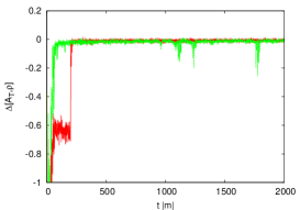
In Fig.3a the time evolution of this quantity is displayed in two characteristic runs. In the first a large negative value is reached almost instantly after the Higgs-field rolls down. After a longer time interval Δ[𝐀T,ρ]Δsubscript𝐀𝑇𝜌\Delta[{\bf A}_{T},\rho] suddenly jumps to a value compatible with zero. In the other run one can observe negative ”needles” occuring on the background of near-zero fluctuations.

A large negative value of the correlation coefficient (4) represents a very sensitive indicator for the presence of relativistic Abrikosov-strings. The location of the points where ρ/|m|<0.3𝜌𝑚0.3\rho/|m|<0.3 displays a vortex network very nicely (see Fig. 3b), but Δ0Δ0\Delta\approx 0 excludes the presence of vortices.

Refer to captionRefer to caption

Figure 3: Non-smooth 𝐀Tρsubscript𝐀𝑇𝜌{\bf A}_{T}-\rho correlation histories, and the corresponding vortex pair.

The longitudinal polarisation. The quantity Δ[𝐀L,ρ]Δsubscript𝐀𝐿𝜌\Delta[{\bf A}_{L},\rho] always displays instantly after the roll-down values significantly different from zero. and shows only a very mild time variation. It was checked that a non-zero value is present also in equilibrium [4]. This correlation coeficient linearly increases with the temperature. These observations point to the fact that the true quasiparticle field is a composite of ρ𝜌\rho and 𝐀Lsubscript𝐀𝐿{\bf A}_{L}. This is not a very great surprise for relatively strongly coupled systems, still it should be confronted with the fact that (without vortices) 𝐀T(𝐤,t)subscript𝐀𝑇𝐤𝑡{\bf A}_{T}({\bf k},t) and ρ(𝐤,t)𝜌𝐤𝑡\rho({\bf k},t) perform statistically independent and Gaussian small oscillations.
Refer to caption

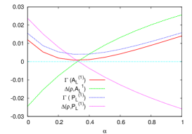
Figure 4: Correlations testing independence and Gaussianity of (5) in function of α𝛼\alpha

We have tested several trial composite fields at equilibrium [4]. In Fig. 4 we show the variation of Δ[PL,ρ],Δ[QL,ρ]Δsubscript𝑃𝐿𝜌Δsubscript𝑄𝐿𝜌\Delta[P_{L},\rho],\Delta[Q_{L},\rho] and of Γ[PL],Γ[QL]Γdelimited-[]subscript𝑃𝐿Γdelimited-[]subscript𝑄𝐿\Gamma[P_{L}],\Gamma[Q_{L}] defined by the ratio Γ[QL]((QL2(𝐱,t))2¯3(QL2(𝐱,t)¯)2)/(QL2(𝐱,t))2¯Γdelimited-[]subscript𝑄𝐿¯superscriptsuperscriptsubscript𝑄𝐿2𝐱𝑡23superscript¯superscriptsubscript𝑄𝐿2𝐱𝑡2¯superscriptsuperscriptsubscript𝑄𝐿2𝐱𝑡2\Gamma[Q_{L}]\equiv\left({\overline{\left(Q_{L}^{2}({\bf x},t)\right)^{2}}-3\left(\overline{Q_{L}^{2}({\bf x},t)}\right)^{2}}\right)/\overline{\left(Q_{L}^{2}({\bf x},t)\right)^{2}} as a function of α𝛼\alpha which characterizes the compositeness of the conjugate variables

QL(𝐱,t)=(1+αρ2(𝐱,t))𝐀L(𝐱,t),PL(𝐱,t)=ΠL(𝐱,t)/(1+αρ2(𝐱,t)).formulae-sequencesubscript𝑄𝐿𝐱𝑡1𝛼superscript𝜌2𝐱𝑡subscript𝐀𝐿𝐱𝑡subscript𝑃𝐿𝐱𝑡subscriptΠ𝐿𝐱𝑡1𝛼superscript𝜌2𝐱𝑡Q_{L}({\bf x},t)=(1+\alpha\rho^{2}({\bf x},t)){\bf A}_{L}({\bf x},t),\quad P_{L}({\bf x},t)=\Pi_{L}({\bf x},t)/(1+\alpha\rho^{2}({\bf x},t)). (5)

The coefficients ΓΓ\Gamma signal deviations from Gaussianity. The nice surprise is that in equilibrium there exists a single optimal choice αoptsubscript𝛼𝑜𝑝𝑡\alpha_{opt} where Δ[PL,ρ],Δ[QL,ρ]Δsubscript𝑃𝐿𝜌Δsubscript𝑄𝐿𝜌\Delta[P_{L},\rho],\Delta[Q_{L},\rho] vanish and both ΓΓ\Gamma’s are minimal. It turns out, however, that during the non-equilibrium phase transition no such αoptsubscript𝛼𝑜𝑝𝑡\alpha_{opt} appears to exist, the ”longitudinal quasiparticle” coordinate presumably emerges only on the thermalisation scale.

In conclusion, we found that in the abelian Higgs model an early quasi-particle characterisation works well for the dispersion relations and the equations of state just after the symmetry breaking is completed. The non-linear quasi-particle field containing the longitudinal vector component builds up much more slowly in the process of complete thermalisation.

References

  • [1] J. Smit, Cold Electroweak Baryogenesis, to appear in Proc. of SEWM’04
  • [2] J.-I. Skullerud, J. Smit and A. Tranberg, JHEP 0308 (2003) 045
  • [3] M. Hindmarsh and A. Rajantie, Phys. Rev. D64 (2001) 065016
  • [4] D. Sexty and A. Patkós, hep-ph/0404235
  • [5] J. Berges, Sz. Borsányi, C. Wetterich,hep-ph/0403234