The mass of the nucleon in a chiral quark-diquark model

The mass of the nucleon is studied in a chiral quark-diquark model. Both scalar and axial-vector diquarks are taken into account for the construction of the nucleon state. After the hadronization procedure to obtain an effective meson-baryon Lagrangian, the quark-diquark self-energy is calculated in order to generate the baryon kinetic term as well as the mass of the nucleon. It turns out that both the scalar and axial-vector parts of the self-energy are attractive for the mass of the nucleon. We investigate the range of parameters that can reproduce the mass of the nucleon.

1 Introduction

An effective Lagrangian approach is an useful method for the description of hadron properties at low energies. Such a Lagrangian contains various terms and parameters expressing not only structures of mesons and baryons but also their interactions. A microscopic description for such terms is desired, especially when we consider, for instance, character changes of hadrons at finite temperatures and densities, which is one of the interesting topics of current hadron physics.

Eventually, QCD should address this issue, but the present situation is not very satisfactory. If we start, however, from an intermediate QCD oriented theory, we can make a reasonably good achievement. One of such approach is the Nambu-Jona-Lasinio model [1, 2, 3] for mesons, and the quark diquark model for mesons and baryons [4, 5]. The models have been tested to a great extent for the description of various meson and baryon properties. It was then shown that the hadronization method based on the path-integral formalism is useful, because it can incorporate hadron structure in terms of quarks and diquarks with respecting important symmetries such as the gauge and chiral symmetries. This idea was first investigated by Cahill [6] and Reinhardt [7]. This, then, was also investigated by Ebert and Jurke in a simplified framework [4], which was later more elaborated by Abu-Raddad et al [5]. Recently, the method was applied also to the nuclear force by the present authors [8]. Nonetheless, these previous studies were done only with the scalar diquark, though the construction of the baryon requires two types of diquarks: scalar and axial-vector ones. The inclusion of the axial-vector diquarks is crucially important for the description of spin-isospin quantities such as the axial coupling constant $g_{A}$ and isovector magnetic moment $\mu$ of the nucleon, and also the nuclear force.

In this paper, we extend our previous study and calculate the nucleon mass with the inclusion of the axial-vector diquark. This is a necessary step to complete the program of the hadronization method. It is shown that by choosing suitable parameters, the mass of the nucleon is reproduced with the same significant amount of the axial-vector diquark component, which will help improve the observables such as $g_{A}$ and isovector magnetic moment.

The paper is organized as follows. In section 2, we construct a microscopic (quark-diquark) Lagrangian and derive the macroscopic (meson-baryon) Lagrangian through the hadronization of the microscopic Lagrangian. In section 3, we study the quark-diquark self-energy and calculate the mass of the nucleon. In section 4, we present numerical results. The final section is devoted to summary and conclusions.

2 Lagrangian

We briefly review the method to derive the effective meson-baryon Lagrangian following the work of Abu-Raddad et al [5]. Let us start from the SU(2)${}_{L}\times$SU(2)_R NJL Lagrangian

$${\cal L}_{NJL}=\bar{q}(i/{\partial}-m_{0})q+\frac{G}{2}\left[(\bar{q}q)^{2}+(\bar{q}i\gamma_{5}\vec{\tau}q)^{2}\right],$$ (2.1)

where $q$ is the current quark field, ${\tau}_{a}(a=1,2,3)$ the flavor Pauli matrices, $G$ the NJL coupling constant with dimension of (mass)^-2 and $m_{0}$ the current quark mass. In this paper, we set $m_{0}=0$ for simplicity. The NJL Lagrangian is bosonized by introducing collective meson fields as auxiliary fields in the path-integral method. As an intermediate step, we find the following Lagrangian:

$${{\cal L}^{\prime}_{q\sigma\pi}}=\bar{q}\left(i\hbox to0.0pt{/\hss}\partial-g(\sigma+i\gamma_{5}\vec{\tau}\cdot\vec{\pi})\right)q-\frac{g^{2}}{2G}(\sigma^{2}+\vec{\pi}^{\;2})\,.$$ (2.2)

Here $\sigma$ and $\vec{\pi}$ are properly normalized scalar-isoscalar sigma and pseudoscalar-isovector pion fields as generated from $\sigma\sim\bar{q}q$ and $\vec{\pi}\sim i\bar{q}\vec{\tau}\gamma_{5}q$, respectively, and $g$ is a meson-quark coupling constant.

For our purpose, it is convenient to work in the non-linear basis [4, 9, 10]. Firstly, the meson fields are expressed as

$$\sigma+i\gamma_{5}\vec{\tau}\cdot\vec{\pi}=f\exp\left(-\frac{i}{F_{\pi}}\gamma_{5}\vec{\tau}\cdot\vec{\Phi}\right).$$ (2.3)

where $f$ and $\Phi$ are new meson fields in the non-linear basis and $f^{2}=\sigma^{2}+\vec{\pi}^{\;2}$. Spontaneous breaking of chiral symmetry is realized when $f$ takes a non-zero vacuum expectation value $\langle f\rangle=F_{\pi}$, which is identified with the pion decay constant$\sim$ 93 MeV, generating the constituent quark mass dynamically, $m_{q}=gF_{\pi}$ [11]. The non-linear Lagrangian is, then, achieved by chiral rotation from the current ($q$) to constituent ($\chi$) quark fields:

$$\chi=\xi_{5}^{\dagger}q\,,\;\;\;\;\xi_{5}=\exp\left(\frac{i}{2F_{\pi}}\gamma_{5}\vec{\tau}\cdot\vec{\Phi}\right)\,.$$ (2.4)

Thus we find

$${\cal L^{\prime}_{\chi\sigma\pi}}=\bar{\chi}\left(i\hbox to0.0pt{/\hss}\partial-m_{q}-\hbox to0.0pt{/\hss}v-\hbox to0.0pt{/\hss}a\gamma_{5}\right)\chi-\frac{1}{2G}f^{2}\,,$$ (2.5)

where

$$v_{\mu}=\frac{1}{2i}\left(\xi^{\dagger}\partial_{\mu}\xi+\xi\partial_{\mu}\xi^{\dagger}\right)\,,\;\;\;a_{\mu}=\frac{1}{2i}\left(\xi^{\dagger}\partial_{\mu}\xi-\xi\partial_{\mu}\xi^{\dagger}\right)\,,$$ (2.6)

are the vector and axial-vector currents written in terms of the chiral field

$$\xi=\exp\left(\frac{i}{2F_{\pi}}\vec{\tau}\cdot\vec{\Phi}\right).$$ (2.7)

The Lagrangian (2.5) describes not only the kinetic term of the quark, but also quark-meson interactions such as the Yukawa and the Weinberg-Tomozawa types among others.

For the description of baryons, we introduce diquarks and their interactions with quarks. We assume local interactions between a quark and a diquark to generate the nucleon field. As suggested previously [12], we consider two diquarks; one is a Lorentz scalar, isoscalar color $\bar{3}$ one as denoted by $D$, and the other is an axial-vector, isovector color $\bar{3}$ one, $D_{\mu}$. The ground state nucleon is then described as a superposition of the bound state of a quark and scalar diquark ($\equiv$ scalar channel), and the bound state of a quark and axial-vector diquark ($\equiv$ axial-vector channel). Hence, our microscopic Lagrangian for quarks, diquarks and mesons is given by [5]

$${\cal L} = \bar{\chi}(i\hbox to0.0pt{/\hss}\partial-m_{q}-\hbox to0.0pt{/\hss}v-\hbox to0.0pt{/\hss}a\gamma_{5})\chi\;-\;\frac{g^{2}}{2G}f^{2}\;+D^{\dagger}(\partial^{2}+M_{S}^{2})D\;+\;{\vec{D}^{{\dagger}\;\mu}}\left[(\partial^{2}+M_{A}^{2})g_{\mu\nu}-\partial_{\mu}\partial_{\nu}\right]\vec{D}^{\nu}$$ (2.8)

$$\;+\;\tilde{G}\left(\sin{\theta}\;\bar{\chi}\gamma^{\mu}\gamma^{5}\>\vec{\tau}\cdot{\vec{D}}^{\dagger}_{\mu}\;+\;\cos{\theta}\;\bar{\chi}D^{\dagger}\right)\;\left(\sin{\theta}\;{\vec{D}}_{\nu}\cdot\vec{\tau}\>\gamma^{\nu}\gamma^{5}\chi\;+\;\cos{\theta}\;D\chi\right)\;.$$

In the last term $\tilde{G}$ is a coupling constant for the quark-diquark interaction and an angle $\theta$ controls the mixing ratio of the scalar and axial-vector channels in the nucleon wave function. In this construction, we have assumed a local interaction between the quark and diquarks. This stems from, for instance, the static limit of a quark exchange between a quark and a diquark as shown in Fig.1. In this case, due to the spin-flavor-color structure, the interactions become attractive both for the scalar and axial-vector diquark channels. In Eq. (2.8), a positive $\tilde{G}$ guarantees an attractive interaction, which is the case we consider.

Now the hadronization procedure is straightforward by the introduction of a baryon field as an auxiliary field $B\sim\sin\theta\vec{D}_{\nu}\cdot\vec{\tau}\gamma^{\nu}\gamma_{5}\chi+\cos\theta D\chi$ and the elimination of the quark and diquark fields in Eq. (2.8). The final result is written in a compact form as [5]

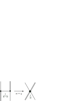
Figure 1: The quark exchange diagram(left) in the Faddeev approach [13, 14] and its static limit(right).

$${\cal L}_{\rm eff} = -\frac{1}{2G}f^{2}\;-\;i\;{\rm tr\;ln}(i\hbox to0.0pt{/\hss}\partial-m_{q}-\hbox to0.0pt{/\hss}v-\hbox to0.0pt{/\hss}a\gamma_{5})\;-\;\frac{1}{\tilde{G}}\;\bar{B}B\;+\;i\;{\rm tr\;ln}(1\;-\;\Box)\,.$$ (2.9)

Here traces are taken over space-time, color, flavor, and Lorentz indices, and the operator $\Box$ is defined by

$$\Box = \begin{pmatrix}{\cal A}&{{\cal F}_{2}}\\ {{\cal F}_{1}}&{\cal S}\end{pmatrix}\,,$$ (2.10)

where

$${\cal A}^{\mu i,\,\nu j} = {\sin}^{2}\theta\ \bar{B}\;\gamma_{\rho}\gamma^{5}\;{\tau}_{k}\;\tilde{\Delta}^{\rho k,\,\mu i}\;S\;{\tau}^{j}\;\gamma^{\nu}\gamma^{5}\;B\;,$$ (2.11a)

$${\cal S} = {\cos}^{2}\theta\;\bar{B}\;\Delta\;S\;B\;,\;\;\;\;\;\;$$ (2.11b)

$$({{\cal F}}_{1})^{\nu j} = \sin{\theta}\cos{\theta}\;\bar{B}\;\Delta\;S\;{\tau^{j}}\;\gamma^{\nu}\gamma^{5}\;B\;,$$ (2.11c)

$$({\cal F}_{2})^{\mu i} = \sin{\theta}\cos{\theta}\;\;\bar{B}\;\tilde{\Delta}^{\rho k,\,\mu i}\;\gamma_{\rho}\gamma^{5}\;{\tau_{k}}\;S\;B\;.$$ (2.11d)

The $S$, $\Delta$ and $\tilde{\Delta}$ are the quark, scalar diquark and axial-vector diquark propagators. The tr log can be expanded as

$$\,\hbox{tr}\,\mbox{ln}(1-\Box)=-\,\hbox{tr}\,\left(\Box+\frac{\Box^{2}}{2}+\cdots\right).$$ (2.12)

The first term on the right hand side describes one particle properties of the nucleon, as it contains the nucleon bilinear form $\bar{B}\Gamma B$, while higher order terms contain two, three and more nucleon interaction terms.

Finally, we comment on the properties of the nucleon field. Since we take the non-linear representation, the transformation properties of baryons under chiral $SU(2)_{L}\times SU(2)_{R}$ are simple. Baryons transform in the same way as quarks do

$$\chi\to\chi^{\prime}(x)=h(x)\chi(x),B(x)\to B^{\prime}(x)=h(x)B(x),$$ (2.13)

where $h(x)$ is the non-linear function of the chiral transformations and of the chiral field at a point $x$ [10]. Here we note that the baryon field $B(x)$, in terms of quarks and diquarks, is related to the nucleon wave-function in the constituent quark model by way of

$$D\chi=2\phi_{\rho}\chi_{\rho},$$ (2.14)

$$\vec{D}_{\nu}\cdot\vec{\tau}\gamma^{\nu}\gamma_{5}\chi=6\phi_{\lambda}\chi_{\lambda},$$ (2.15)

in the non-relativistic limit, where $\phi_{\rho},\ \phi_{\lambda}$ and $\chi_{\rho},\ \chi_{\lambda}$ are the standard 3-quark spin and iso-spin wave-functions [10]. If we take $\tan\theta=1/3$, we realize the $SU(4)$ spin-flavor symmetry of the constituent quark model.

3 The quark-diquark self-energy

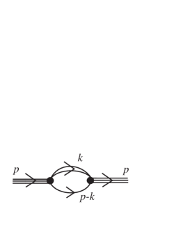
Figure 2: A diagrammatic representation of the quark-diquark self-energy. The single, double and triple lines represent the quark, diquark and nucleon respectively.

In the first order term with respect to $\Box$ of Eq. (2.12), the quark-diquark self-energy corresponding to Fig. 2 is given by,

$${\cal L}_{0}=-i\,\hbox{tr}\,\left[{\cal S}+{\cal A}^{\mu\nu}_{ij}\right]-\frac{1}{\tilde{G}}\bar{B}B.$$ (3.1)

Using the interaction terms in Eqs. (2.11), we obtain

$${\cal L}_{0}=\cos^{2}\theta\bar{B}(p)\Sigma_{S}(p)B(p)+\sin^{2}\theta\bar{B}(p)\Sigma_{A}(p)B(p)-\frac{1}{\tilde{G}}\bar{B}B,$$ (3.2)

where $\Sigma_{S}(p)$ and $\Sigma_{A}(p)$ are the nucleon self-energies corresponding to the scalar and axial-vector diquark channels, respectively,

$$\Sigma_{S}(p) = -iN_{c}\int\frac{d^{4}k}{(2\pi)^{4}}\frac{1}{k^{2}-M_{S}^{2}}\frac{/{p}-/{k}+m_{q}}{(p-k)^{2}-m_{q}^{2}},$$ (3.3a)

$$\Sigma_{A}(p) = -iN_{c}\int\frac{d^{4}k}{(2\pi)^{4}}\frac{k^{\mu}k^{\nu}/M_{A}^{2}-g^{\mu\nu}}{k^{2}-M_{A}^{2}}\delta_{ij}\gamma_{\nu}\gamma_{5}\tau_{j}\frac{/{p}-/{k}+m_{q}}{(p-k)^{2}-m_{q}^{2}}\tau_{i}\gamma_{\mu}\gamma_{5}.$$ (3.3b)

These are divergent; $\Sigma_{S}(p)$ is logarithmically and $\Sigma_{A}(p)$ quadratically divergent. In the previous works, we employed the Pauli-Villars regularization to let the divergences finite. In the present work, however we shall employ the three momentum cutoff method, since the Pauli-Villars method is not appropriate to regularize the quadratic divergence in $\Sigma_{A}$. The quadratic nature necessarily requires two independent cutoff parameters in the Pauli-Villars method, while it is sufficient to introduce single cutoff parameter in the three-momentum cut-off scheme.

Now in the rest frame of the nucleon, i.e. $p=(p_{0},\vec{0})$, the self-energies as functions of $p_{0}$ can be written as, after integrating Eqs. (3.3) over $k_{0}$,

$$\Sigma_{S}(p_{0}) = \Sigma_{S}^{0}(p_{0})+\Sigma^{1}_{S}(p_{0})\gamma_{0}\,,$$

$$\Sigma_{A}(p_{0}) = \Sigma_{A}^{0}(p_{0})+\Sigma^{1}_{A}(p_{0})\gamma_{0}\,,$$ (3.4)

where the coefficients are given as

$$\Sigma_{S}^{0}(p_{0}) = -N_{c}\int_{0}^{\Lambda}\frac{k^{2}dk}{2\pi^{2}}\left\{\frac{m_{q}}{2e_{1}[(p_{0}+e_{1})^{2}-e_{2}^{2}]}+\frac{m_{q}}{2e_{2}[(p_{0}-e_{2})^{2}-e_{1}^{2}]}\right\}_{,}$$

$$\Sigma_{S}^{1}(p_{0}) = -N_{c}\int_{0}^{\Lambda}\frac{k^{2}dk}{2\pi^{2}}\left\{\frac{-e_{1}}{2e_{1}[(p_{0}+e_{1})^{2}-e_{2}^{2}]}+\frac{(p_{0}-e_{2})}{2e_{2}[(p_{0}-e_{2})^{2}-e_{1}^{2}]}\right\}_{,}$$ (3.5)

and

$$\Sigma_{A}^{0}(p_{0}) = -\frac{N_{c}\vec{\tau}^{2}}{M_{A}^{2}}\int_{0}^{\Lambda}\frac{k^{2}dk}{2\pi^{2}}\left\{\frac{3m_{q}M_{A}^{2}}{2e_{3}[(e_{3}-p_{0})^{2}-e_{1}^{2}]}\right.$$

$$+\;\left.\frac{4m_{q}M_{A}^{2}-m_{q}\left((p_{0}+e_{1})^{2}-\vec{k}^{2}\right)}{2e_{1}[(p_{0}+e_{1})^{2}-e_{3}^{2}]}\right\}\,,$$

$$\Sigma_{A}^{1}(p_{0}) = -\frac{N_{c}\vec{\tau}^{2}}{M_{A}^{2}}\int_{0}^{\Lambda}\frac{k^{2}dk}{2\pi^{2}}\left\{\frac{-3e_{3}M_{A}^{2}+p_{0}M_{A}^{2}+2e_{3}^{2}p_{0}}{2e_{3}[(e_{3}-p_{0})^{2}-e_{1}^{2}]}\right.$$ (3.6)

$$+\;\left.\frac{-2e_{1}M_{A}^{2}-e_{1}(p_{0}+e_{1})^{2}+(2p_{0}+e_{1})\vec{k}^{2}}{2e_{1}[(p_{0}+e_{1})^{2}-e_{3}^{2}]}\right\}\,.$$

In the above equations $N_{c}$ is the number of colors, and $e_{1}=\sqrt{\vec{k}^{2}+m_{q}^{2}},e_{2}=\sqrt{\vec{k}^{2}+M_{S}^{2}},e_{3}=\sqrt{\vec{k}^{2}+M_{A}^{2}}$.

Now physical nucleon fields are defined such that the self-energy becomes the nucleon propagator on the nucleon mass shell. This condition is implemented by expanding the self-energy around $p_{0}=M_{N}$:

$$\bar{B}\left(\cos^{2}\theta\Sigma_{S}(p_{0})+\sin^{2}\theta\Sigma_{A}(p_{0})-\frac{1}{\tilde{G}}\right)B = Z^{-1}\bar{B}(p_{0}\gamma^{0}-M_{N})B$$ (3.7)

$$= \bar{B}_{phys}(p_{0}\gamma^{0}-M_{N})B_{phys},$$

where $B_{phys}=\sqrt{Z^{-1}}B$ is the properly normalized physical nucleon field. The parameters $Z$ and $M_{N}$ are the wave-function renormalization constant and the mass of the nucleon. The parameters $Z$, $M_{N}$ and $\tilde{G}$ are determined by the following conditions,

$$Z^{-1} = \left.\frac{\partial\Sigma(p_{0})}{\partial p_{0}}\right|_{p_{0}\to M_{N}}=\cos^{2}\theta\frac{\partial\Sigma_{S}(M_{N})}{\partial p_{0}}+\sin^{2}\theta\frac{\partial\Sigma_{A}(M_{N})}{\partial p_{0}}_{,}$$ (3.8)

$$\tilde{G} = (\cos^{2}\theta\Sigma_{S}(M_{N})+\sin^{2}\theta\Sigma_{A}(M_{N}))^{-1}_{.}$$ (3.9)

Therefore, we obtain the mass of the physical nucleon by solving Eqs. (3.8) and (3.9).

4 Results

To start with, we briefly discuss our parameters which are listed in Table 1. We use the values in Ref. [5] for the mass of the constituent quarks $m_{q}$, the NJL coupling constant $G$ and the cut-off mass $\Lambda$. Then $m_{q}$, $G$ and $\Lambda$ are determined self-consistently in the NJL model by solving the gap equation and reproducing the pion decay constant $f_{\pi}=93$ MeV [11, 15, 2]. The masses of the scalar and axial-vector diquarks, $M_{S}$ and $M_{A}$ may be determined , for instance, in the NJL model by solving the Bethe-Salpeter equation in the corresponding diquark channels [3, 16]. These masses have been also calculated by QCD oriented methods [17, 18, 19]. Results are, however, somewhat dependent on the methods. Here, instead of solving the BS equation rigorously, we simply choose a reasonable set of diquark masses. These parameters can reproduce, for instance the mass splitting between the nucleon and delta[3, 17].

Table 1: Model parameters. All parameters are in units of GeV.

$m_{q}$	$M_{S}$	$M_{A}$	$\Lambda$
0.39	0.60	1.05	0.6

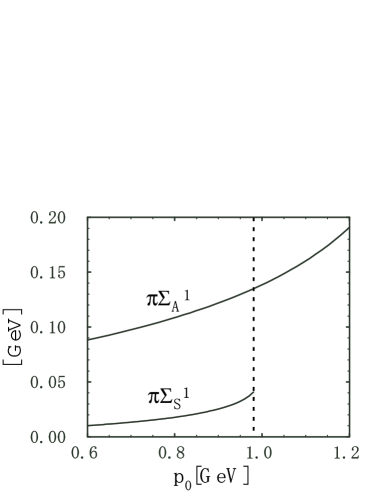
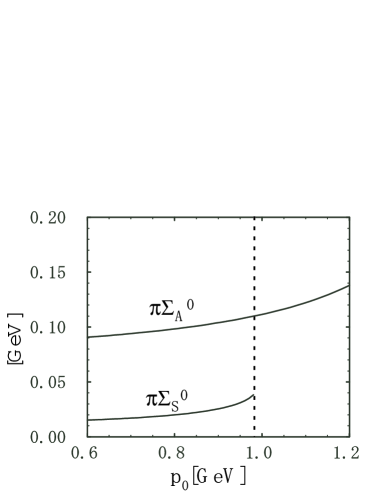
Figure 3: Real parts of the self-energies $\Sigma_{S,A}^{1}$(left) and $\Sigma_{S,A}^{0}$(right) multiplied by $\pi$. The vertical dashed lines represent the threshold for the quark and scalar diquark channel $=m_{q}+M_{S}$.

In Fig. 3, we plotted the real parts of the self-energies Eqs. (3.5) and (3.6) as functions of $p_{0}$.

We find that both scalar and axial-vector channels are positive, meaning that both channels contribute to the mass of the nucleon attractively, or decrease the mass of the nucleon. Obviously the contributions of the axial-vector diquark part is considerably larger than that of the scalar diquark part, reflecting the stronger (quadratic) divergence of the former than the latter. In Fig. 3 we also explicitly show a threshold $m_{q}+M_{S}$. We can not obtain the reasonable result for the larger mass of $M_{N}$ than $m_{q}+M_{S}$, because this model has no confining effect. Recently, several works including the mimic effects of the confinement was done[20, 21, 22]. Although we continue this simple treatment, we should confine this model in the region $M_{N}<m_{q}+M_{S}$.

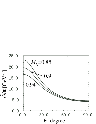
Figure 4: The contour plot of the nucleon mass $M_{N}$ as a function of the coupling constant $\tilde{G}$ (divided by $\pi$) and the mixing angle $\theta$. Each lines are for $M_{N}$=0.94, 0.90, 0.85 [GeV] from bottom to top.

In this paper, the mass of the nucleon $M_{N}$ is treated as a function of $\tilde{G}$ and the mixing angle $\theta$. In Fig. 4, we show the contour plot for the nucleon mass as a function of $\tilde{G}$ and $\theta$. One finds that both of the scalar and axial-vector parts of the self-energy contribute attractively to the mass of the nucleon, and that the attraction from the axial part is larger than that from the scalar part. At $\theta=0$ where only $\Sigma_{S}$ contributes to the mass of the nucleon, the experimental value $M_{N}=0.94$ GeV is obtained when $\tilde{G}/\pi\sim 17$. In making comparisons, we note that in the present calculation pion cloud effect is not included, which might bring substantial contribution to nucleon properties at the quantitative level [23, 24, 25]. Nevertheless, for the qualitative discussions in the present paper, we simply compare the results with experiments directly.

At $\theta=30$ degrees, for instance, the mass of the nucleon is reproduced when $\tilde{G}/\pi\sim 9.5$. As the mixing angle $\theta$ increases, or the axial-vector component in the nucleon wave-function becomes larger, the mass of the nucleon decreases. This behavior is also shown in Fig. 5, where $\theta$ dependence is shown for fixed values of $\tilde{G}$. One sees that for larger values of $\theta$, $M_{N}$ is reproduced for smaller values of $\tilde{G}$, showing once again that the attraction from the axial-vector part is larger than the attraction in the scalar part. Although we do not discuss in this paper, a finite value of $\theta$ is favored when explaining the isovector magnetic moments $\mu$ and isovector axial-vector coupling constant $g_{A}$.

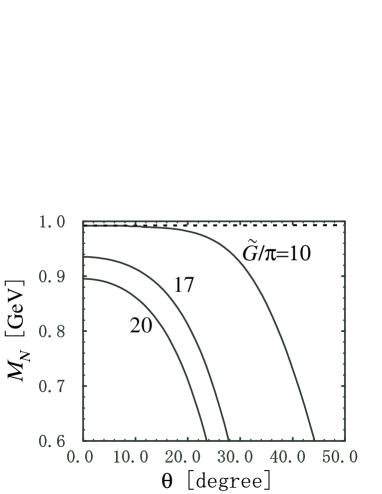
Figure 5: The mixing angle $\theta$ dependence of the mass of the nucleon $M_{N}$ for several values of the quark-diquark coupling constant $\tilde{G}$. Three curves are for $\tilde{G}/\pi$=20, 17, 10 [GeV^-1] from bottom to top as indicated. Dashed horizontal line is the threshold $=m_{q}+M_{S}$.

5 Summary

In this paper, we have studied the nucleon state in terms of a microscopic model for hadrons, namely, a chiral quark-diquark model. The nucleon was constructed as a superposition of the two quark-diquark channels including the scalar and axial-vector diquarks. The quark-diquark model was then hadronized in the path-integral method to obtain an effective Lagrangian for the mesons and nucleon. The present work is an extension of the previous ones including only scalar diquark channel. Here, in order to test the validity of the method and see a role the axial-vector diquark channel plays, we investigated the mass of the nucleon. It was calculated through the renormalization conditions of the nucleon self-energies. Then we found that the mass of the nucleon is reproduced by choosing the mixing angle $\theta$ and the coupling constant $\tilde{G}$ appropriately. Our result is consistent with the previous work solving the Faddeev equations for the three quark system in the NJL model [14].

The present result suggests that the quark-diquark model, although it is simpler than solving the three quark system directly, would be a practically useful model for the description of the nucleon. As advocated previously, an advantage of the present method is to be able to work out to a large extent in an analytic way preserving important symmetries such as gauge and chiral symmetries.

Naturally, it is a further extension to apply the present method to various hadronic properties such as the electromagnetic couplings and the nuclear force. For some quantities such as isovector magnetic moments and axial-vector coupling constants, it is expected that the axial-vector channel play an important role [26, 27]. Furthermore, this is necessary to describe the octet and decuplet baryons. In addition, the axial-vector channel may play another role which we did not consider explicitly in the present work, for only a single state of the nucleon was constructed. If both the channels are treated as independent degrees of freedom, then the two nucleon states may be described as bound states of the quark and diquarks. This is investigated in a separate paper [28].

Note added

In the numerical calculation of the self-energies in the original version, the factor $\pi$ was missed. In order to account for the factor correctly, the self-energies shown in Fig. 3 and the coupling constant $\tilde{G}$ are scaled by the factor $\pi$. The results and conclusions are not affected. This is reported in Erratum of PRC.

References

- [1] Y. Nambu and G. Jona-Lasinio, Phys. Rev. 122, 345 (1961); ibid. 124, 246 (1961).
- [2] T. Hatsuda and T. Kunihiro, Phys. Rept. 247, 221 (1994).
- [3] U. Vogl and W. Weise, Prog. Part. Nucl. Phys. 27, 195 (1991).
- [4] D. Ebert and T. Jurke, Phys. Rev. D 58, 034001(1998).
- [5] L. J. Abu-Raddad, A. Hosaka, D. Ebert and H. Toki, Phys. Rev. C 66, 025206 (2002).
- [6] R. T. Cahill, Austral. J. Phys. 42, 171 (1989).
- [7] H. Reinhardt, Phys. Lett. B 244, 316 (1990).
- [8] K. Nagata and A. Hosaka, Prog. Theor. Phys. 111, 857 (2004).
- [9] N. Ishii, Nucl. Phys. A 689, 793 (2001).
- [10] A. Hosaka and H. Toki, Quarks, Baryons and Chiral Symmetry, World Scientific (2001).
- [11] D. Ebert and H. Reinhardt, Nucl. Phys. B 271, 188 (1986).
- [12] D. Espriu, P. Pascual and R. Tarrach, Nucl. Phys. B 214, 285 (1983).
- [13] A. Buck, R. Alkofer and H. Reinhardt, Phys. Lett. B 286, 29 (1992).
- [14] N. Ishii, W. Bentz and K. Yazaki, Phys. Lett. B 318, 26 (1993).
- [15] D. Ebert, H. Reinhardt and M. K. Volkov, Prog. Part. Nucl. Phys. 33, 1 (1994).
- [16] R. T. Cahill, C. D. Roberts and J. Praschifka, Phys. Rev. D 36, 2804 (1987).
- [17] M. Hess, F. Karsch, E. Laermann and I. Wetzorke, Phys. Rev. D 58, 111502 (1998).
- [18] P. Maris, Few Body Syst. 32, 41 (2002).
- [19] C. J. Burden, L. Qian, C. D. Roberts, P. C. Tandy and M. J. Thomson, Phys. Rev. C 55, 2649 (1997).
- [20] M. Oettel, G. Hellstern, R. Alkofer and H. Reinhardt, Phys. Rev. C 58, 2459 (1998).
- [21] G. Hellstern, R. Alkofer and H. Reinhardt, Nucl. Phys. A 625, 697 (1997).
- [22] G. Hellstern, R. Alkofer, M. Oettel and H. Reinhardt, Nucl. Phys. A 627, 679 (1997).
- [23] A. W. Thomas, Adv. Nucl. Phys. 13, 1 (1984).
- [24] N. Ishii, Phys. Lett. B 431, 1 (1998).
- [25] M. B. Hecht, M. Oettel, C. D. Roberts, S. M. Schmidt, P. C. Tandy and A. W. Thomas, Phys. Rev. C 65, 055204 (2002).
- [26] R. Alkofer, A. Höll, M. Kloker, A. Krassnigg and C. D. Roberts, Few Body Syst. 37, 1 (2005).
- [27] A. Holl, R. Alkofer, M. Kloker, A. Krassnigg, C. D. Roberts and S. V. Wright, Nucl. Phys. A 755, 298 (2005).
- [28] K. Nagata and A. Hosaka, arXiv:hep-ph/0506193.