Abstract
We propose a sophisticated framework for high-energy hadronic collisions, wherein different QCD physics processes are interleaved in a common sequence of falling transverse-momentum values. Thereby phase-space competition is introduced between multiple parton–parton interactions and initial-state radiation. As a first step we develop new transverse-momentum-ordered showers for initial- and final-state radiation, which should be of use also beyond the scope of the current article. These showers are then applied in the context of multiple interactions, and a few tests of the new model are presented. The article concludes with an outlook on further aspects, such as the possibility of a shower branching giving partons participating in two different interactions.

1 Introduction

High-energy hadronic collisions offer a busy environment. The incoming hadrons seethe with activity as partons continuously branch and recombine. At the moment of collision, several partons from the two incoming hadrons may undergo interactions, that scatter the partons in different directions. The scattered partons may radiate, and all outgoing partons, including the beam remnants, hadronize in a correlated fashion to produce the observable high-multiplicity events. The physics involves a subtle blend of many perturbative and nonperturbative phenomena. No wonder that there is no simple, standard description to be offered!

What often saves the day is that most of the above activity is soft, i.e. confined to small transverse momenta $p_{\perp}$. When the processes of interest occur at large momentum transfers they therefore stand out, by producing jets, leptons or photons at large $p_{\perp}$. To first approximation, the rest of the activity, which we refer to as the underlying event, may then be disregarded. For precision studies, however, the problem remains: minijets from the underlying event may e.g. affect the jet energy calibration and the lepton and photon isolation criteria. Quite apart from the interesting challenge of better understanding the complex (semi-)soft processes for their own sake, this motivates an effort to investigate and model as well as possible the underlying event physics (when a selective trigger is used) and minimum-bias physics (for the inclusive sample of multihadronic events).

The basic building blocks needed to describe hadron–hadron collisions include hard-scattering matrix elements, parton density functions, initial- and final-state parton showers, and a hadronization scheme. Each of these deserve study in its own right, but additionally there is the question of how they should be combined. It is this latter aspect that we take aim at here. More specifically, we concentrate on the non-trivial interplay between multiple parton–parton interactions and initial-state parton showers, extending previous models for multiple interactions and developing new models for $p_{\perp}$-ordered initial- and final-state parton showers in the process.

Figure 1: Schematic figure illustrating one incoming hadron in an event with a hard interaction occurring at $p_{\perp 1}$ and three further interactions at successively lower $p_{\perp}$ scales, each associated with (the potentiality of) initial-state radiation, and further with the possibility of two interacting partons (2 and 3 here) having a common ancestor in the parton showers. Full lines represent quarks and spirals gluons. The vertical $p_{\perp}$ scale is chosen for clarity rather than realism; most of the activity is concentrated to small $p_{\perp}$ values.

A good starting point for the discussion is offered by Fig. 1. Based on the composite nature of hadrons we have here depicted multiple interactions (MI) between several pairs of incoming partons, see ref. [1] for a minireview. The structure of an incoming hadron is illustrated, with the $p_{\perp}$ evolution of some partons from a nonperturbative border at $p_{\perp\mathrm{min}}$ up to the different perturbative interactions. The $p^{2}_{\perp}=\hat{t}\hat{u}/\hat{s}$ scale is a convenient measure of hardness, since the $t$ (and $u$) channel gluon exchange processes $\mathrm{q}\mathrm{q}^{\prime}\to\mathrm{q}\mathrm{q}^{\prime}$, $\mathrm{q}\mathrm{g}\to\mathrm{q}\mathrm{g}$ and $\mathrm{g}\mathrm{g}\to\mathrm{g}\mathrm{g}$ dominate the cross section. One has to imagine a corresponding picture for the other hadron — omitted for clarity — with the two incoming sides joined at the interactions.

The next immediate issue that arises is how to describe hadronic objects under such conditions. In general, cross section calculations rely on parton density functions to describe the initial state. For the joint cross section of several simultaneous interactions one thus needs multi-parton densities, categorized by flavour content and fully differential in all $x$ and $Q^{2}\approx p^{2}_{\perp}$ values. Obviously such densities are almost entirely unconstrained, with neither data nor first-principles theory giving more than the roughest guidelines. To develop a realistic approximate framework, it is natural to consider first the hardest interaction, which after all should be the most important one in terms of experimental consequences. Moreover, self-consistency ensures that this is also the interaction for which the standard ‘one-parton-inclusive’ pdf’s should be applicable; when averaging over all configurations of softer partons, the standard QCD phenomenology should be obtained for the ones participating in the hardest interaction, this being the way the standard parton densities have been measured. Thus it makes sense to order and study the interactions in a sequence of falling ‘hardness’, for which we shall here take $p_{\perp}$ as our measure, i.e. we consider the interactions in a sequence $p_{\perp 1}>p_{\perp 2}>p_{\perp 3}>p_{\perp 4}$. The normal parton densities can then be used for the scattering at $p_{\perp 1}$, and correlation effects, known or estimated, can be introduced in the choice of ‘subsequent’ lower-$p_{\perp}$ scatterings.

In ref. [1] we developed a new and sophisticated model to take into account such correlations in momentum and flavour. In particular, contrary to the earlier model described in ref. [2], the new model allows for more than one valence quark to be kicked out, and also takes into account the fact that sea quarks come in pairs. The beam remnant structure and colour flow topologies can become quite complicated, and so-called string junctions have to be handled, see [3].

In addition, the more sophisticated machinery allowed a more complete treatment of initial-state radiation (ISR) and final-state radiation (FSR). That is, each simple $2\to 2$ interaction could be embedded in the center of a more complicated $2\to n$ process, $n\geq 2$, where additional partons are produced by ISR or FSR. In order to avoid doublecounting, this additional radiation should be softer than the core $2\to 2$ interaction. Here $p^{2}_{\perp}$ is again a convenient measure for hardness ordering, but not a unique one.

In this article, we introduce an additional interplay, between multiple parton interactions and ISR. ISR is the mechanism whereby parton densities evolve and become scale-dependent. The paradigm is that parton densities at a scale $Q^{2}$, in our case identified with $p^{2}_{\perp}$, probe the resolved partonic content at that scale. Therefore the issue of multi-parton densities is mixed in with the handling of ISR. For instance, if an ISR branching related to the first interaction occurs at a $p_{\perp 1}^{\prime}<p_{\perp 1}$ then that reduces the available phase space for a second interaction at $p_{\perp 2}<p_{\perp 1}^{\prime}$. In the complementary region $p_{\perp 2}>p_{\perp 1}^{\prime}$, it is instead the momentum carried away by the second interaction that reduces the phase space for the ISR branching of the first. Thus, a consistent choice is to consider ISR (on both of the two incoming hadron sides) and MI in parallel, in one common sequence of decreasing $p_{\perp}$ values, where the partonic structure at one $p_{\perp}$ scale defines what is allowed at lower scales. Again this approach of interleaved evolution is intended to accurately reproduce measurements at $p_{\perp}$ values corresponding to the hardest scales in the event, and fits well with the backwards evolution approach to ISR [4]. (One could have devised alternative procedures with forward evolution from lower to higher $p_{\perp}$ values, which would have offered a more intuitive physics picture, but with problems of its own.)

To the best of our knowledge, a scenario of this kind has never before been studied. In the early multiple interactions modelling [2] ISR and FSR was only included for the hardest interaction, and this before additional interactions were at all considered. In our more recent study [1] all interactions included ISR and FSR, but again separately for each interaction.

An additional difference is that, in our previous studies, spacelike (for ISR) or timelike (for FSR) virtuality was used as evolution and ordering variable in the showers. In the framework we shall present here, an essential ingredient is the use of $p_{\perp}$-ordered showers, such that the proposed competition between MI and ISR can be introduced in terms of a common ordering variable. We have therefore completed the rewriting begun in [5] of the existing Pythia showering algorithms [6] to $p_{\perp}$-ordering. These new models have interesting features in their own right, quite apart from the application to interleaved multiple interactions.

This article should be viewed as one step on the way towards a better understanding of hadronic physics, but not as the final word. Further issues abound. The downwards evolution in $p_{\perp}$ may also reveal that two seemingly separately interacting partons actually have a common origin in the branching of a single parton at a lower $p_{\perp}$ scale ($p_{\perp 23}$ in Fig. 1), and a single parton may scatter twice against partons in the other hadron. We shall refer to such possibilities specifically as intertwined multiple interactions, to distinguish them somewhat from the interleaved evolution that will be our main focus here.

In this article we begin, in Section 2, with a description of the new showering framework. This is followed, in Section 3, by a discussion on the model for interleaving MI and ISR, and a few results are presented in Section 4. The outlook in Section 5 contains a first estimate of the significance of the backward evolution joining several interactions. Finally Section 6 gives our conclusions.

2 New Transverse-Momentum-Ordered Showers

In this section we describe the new framework for timelike FSR and spacelike ISR in the context of a single hard-scattering process. We start by a brief review of the main existing showering algorithms, to introduce the basic terminology and ideas we will make use of. Thereafter the philosophy underlying the new algorithms is outlined. The more technical details are then described separately, first for timelike showers and then for spacelike ones, the latter as a rule being the more complicated.

Figure 2: Schematic figure with our standard terminology for (a) a final-state and (b) an initial-state branching $a\to bc$, with a cross marking the central hard process and a recoiling parton $r$ moving out to or coming in from the other side.

2.1 Shower minireview

In the shower approach, the evolution of a complex multi-parton final state is viewed as a succession of simple parton branchings. Thus a $2\to n$ process can be viewed as consisting of a simple high-virtuality process, often $2\to 2$, that approximately defines the directions and energies of the hardest jets of the process, combined with shower branchings at lower virtuality scales. The shower branchings thus add details to the simple answer, both by the production of additional jets and by a broadening of the existing ones. We distinguish between initial-state showers, whereby the incoming partons to the hard process build up increasingly spacelike virtualities $Q^{2}$, and final-state showers, where outgoing partons, including the non-colliding partons emitted from the initial state, may have timelike virtualities $Q^{2}$ that decrease in the cascade down to on-shell partons.

To first order, both cascade types are governed by the same DGLAP evolution equations [7]

$$\mathrm{d}{\cal P}_{a}(z,Q^{2})=\frac{\mathrm{d}Q^{2}}{Q^{2}}\,\frac{\alpha_{\mathrm{s}}}{2\pi}\,P_{a\to bc}(z)\,\mathrm{d}z~{},$$ (1)

expressing the differential probability that a ‘mother’ parton $a$ will branch to two ‘daughter’ partons $b$ and $c$, at a virtuality scale $Q^{2}$, and with parton $b$ taking a fraction $z$ of the $a$ energy, and $c$ a fraction $1-z$, cf. Fig.2. The splitting kernels $P_{a\to bc}(z)$ are (for massless quarks)

$$P_{\mathrm{q}\to\mathrm{q}\mathrm{g}}(z) = \frac{4}{3}\,\frac{1+z^{2}}{1-z}~{},$$ (2)

$$P_{\mathrm{g}\to\mathrm{g}\mathrm{g}}(z) = 3\,\frac{(1-z(1-z))^{2}}{z(1-z)}~{},$$ (3)

$$P_{\mathrm{g}\to\mathrm{q}\overline{\mathrm{q}}}(z) = \frac{n_{f}}{2}\,(z^{2}+(1-z)^{2})~{},$$ (4)

where $n_{f}$ is the number of quark flavours kinematically allowed. The kernels can be viewed as the universal collinear limit of the behaviour of relevant matrix-element expressions. In such a context it is natural to associate $Q^{2}$ with $|m^{2}|$, the virtuality of an intermediate off-shell parton, since a $1/m^{2}$ comes from the propagator of the virtual particle. This is a free choice, however: if $Q^{2}=f(z)\,m^{2}$, then for any (nice) function $f(z)$ it holds that $\mathrm{d}Q^{2}/Q^{2}\,\mathrm{d}z=\mathrm{d}m^{2}/m^{2}\,\mathrm{d}z$. At this stage, several equivalent choices are therefore possible.

Note that eq. (1) formally corresponds to the emission of an infinite number of partons. However, very soft and collinear gluons will not be resolved in an infrared safe fragmentation framework such as the string one [8], so we are free to introduce some effective $Q_{0}$ cut-off scale, of the order of 1 GeV or $\Lambda_{\mathrm{QCD}}$, below which perturbative emissions need not be considered (to first approximation).

The remaining total emission probability is still normally above unity, which is allowed for an inclusive rate since several emissions can occur. For an exclusive parton shower it is then convenient to introduce a ‘time’ ordering, i.e. to decide which of the allowed emissions occur ‘first’. This is encompassed in the Sudakov form factor [9], expressing the probability that no emissions occur between the initial maximum scale $Q^{2}_{\mathrm{max}}$ and a given $Q^{2}$, and within limits $z_{\mathrm{min}}<z<z_{\mathrm{max}}$ that depend on the kinematics and the $Q_{0}$ cutoff,

$${\cal P}^{\mathrm{no}}_{a}(Q^{2}_{\mathrm{max}},Q^{2})=\exp\left(-\int_{Q^{2}}^{Q^{2}_{\mathrm{max}}}\int_{z_{\mathrm{min}}}^{z_{\mathrm{max}}}\mathrm{d}{\cal P}_{a}(z^{\prime},{Q^{\prime}}^{2})\right)~{},$$ (5)

so that the differential probability for the first branching to occur at a $Q^{2}=Q_{a}^{2}$ is given by $\mathrm{d}{\cal P}_{a}(z,Q_{a}^{2})\,{\cal P}^{\mathrm{no}}_{a}(Q^{2}_{\mathrm{max}},Q_{a}^{2})$. Once the parton $a$ has branched, it is now the daughters $b$ and $c$ that can branch in their turn, with their $Q^{2}_{\mathrm{max}}$ given by $Q_{a}^{2}$, and so on until the cutoff scale is reached. Thus the shower builds up.

Obviously, at this stage different $Q^{2}$ choices are no longer equivalent: since $a$ will only branch once, those regions of phase space considered at a later stage will be suppressed by a Sudakov factor relative to those considered earlier.

For ISR, the most commonly adopted approach is that of backwards evolution [4], wherein branchings are reconstructed backwards in time/virtuality from the hard interaction to the shower initiators. The starting point is the DGLAP equation for the $b$ density

$$\mathrm{d}f_{b}(x,Q^{2})=\frac{\mathrm{d}Q^{2}}{Q^{2}}\,\frac{\alpha_{\mathrm{s}}}{2\pi}\,\int\frac{\mathrm{d}x^{\prime}}{x^{\prime}}\,f_{a}(x^{\prime},Q^{2})\,P_{a\to bc}\left(\frac{x}{x^{\prime}}\right)~{}.$$ (6)

This expresses that, during a small increase $\mathrm{d}Q^{2}$ there is a probability for parton $a$ with momentum fraction $x^{\prime}$ to become resolved into parton $b$ at $x=zx^{\prime}$ and another parton $c$ at $x^{\prime}-x=(1-z)x^{\prime}$. Correspondingly, in backwards evolution, during a decrease $\mathrm{d}Q^{2}$ a parton $b$ may become ‘unresolved’ into parton $a$. The relative probability $\mathrm{d}{\cal P}_{b}$ for this to happen is given by the ratio $\mathrm{d}f_{b}/f_{b}$, which translates into

$$\mathrm{d}{\cal P}_{b}(x,Q^{2})=\left|\frac{\mathrm{d}Q^{2}}{Q^{2}}\right|\,\frac{\alpha_{\mathrm{s}}}{2\pi}\,\int\mathrm{d}z\,\frac{x^{\prime}f_{a}(x^{\prime},Q^{2})}{xf_{b}(x,Q^{2})}\,P_{a\to bc}(z)~{}.$$ (7)

Again, ordering the evolution in $Q^{2}$ implies that this ‘naive probability’ should be multiplied by the probability ${\cal P}^{\mathrm{no}}_{b}(x,Q^{2}_{\mathrm{max}},Q^{2})$ for no emissions to occur at scales higher than $Q^{2}$, obtained from $\mathrm{d}{\cal P}_{b}$ by exponentiation like in eq. (5). As for the timelike showers, additional sophistication can be added by coherence constraints and matrix-element merging, but ISR remains less well understood than FSR [22].

2.2 Existing approaches

Of the three most commonly used final-state shower algorithms, Pythia uses $m^{2}$ as evolution variable [10, 11], while Herwig uses an energy-weighted emission angle, $E^{2}(1-\cos\theta)\sim m^{2}/(z(1-z))$ [12], and Ariadne a squared transverse momentum, $\sim z(1-z)m^{2}$ [13, 14, 15]. Thus the three programs give priority to emissions with large invariant mass, large emission angle and large transverse momentum, respectively.

The Herwig algorithm makes angular ordering a direct part of the evolution process, and thereby correctly (in an azimuthal-angle-averaged sense) takes into account coherence effects in the emission of soft gluons [16]. Branchings are not ordered in hardness: often the first emission is that of a soft gluon at wide angles. The algorithm does not populate the full phase space but leaves a ‘dead zone’ in the hard three-jet region, that has to be filled up separately [17]. The kinematics of a shower is only constructed at the very end, after all emissions have been considered.

The Pythia algorithm is chosen such that the shower variables closely match the standard three-jet phase space in $\mathrm{e}^{+}\mathrm{e}^{-}\to\mathrm{q}\overline{\mathrm{q}}\mathrm{g}$, and such that the shower slightly overpopulates the hard three-jet region, so that a simple rejection step can be used to obtain a smooth merging of all relevant first-order gluon-emission matrix elements with the shower description [11]. The mass-ordering of emissions is one possible definition of hardness-ordering. The main limitation of the algorithm is that it does not automatically include coherence effects. Therefore angular ordering is imposed by an additional veto, but then cuts away a bit too much of the soft-gluon phase space [18]. The kinematics of a branching is not constructed until the daughters have been evolved in their turn, so that their virtualities are also known.

The Ariadne algorithm differs from the above two in that it is formulated in terms of dipoles, consisting of parton pairs, rather than in terms of individual partons. The two partons that make up a dipole may then collectively emit a gluon, causing the dipole to split in two. Thus the basic process is that of one dipole branching into two dipoles, rather than of one parton branching into two partons. Emissions are ordered in terms of a decreasing transverse momentum, which automatically includes coherence effects [13], and also is a good measure of hardness. Kinematics can be constructed, in a Lorentz invariant fashion, immediately after each branching, with individual partons kept on mass shell at each stage. This makes it easy to stop and restart the shower at some intermediate $p_{\perp}$ scale. The implementation of an (L)CKKW-style matching of matrix elements with parton showers [19] is therefore simplified, and in particular Sudakov factors can be generated dynamically to take into account the full kinematics of the branching history. A disadvantage is that $\mathrm{g}\to\mathrm{q}\overline{\mathrm{q}}$ branchings do not fit naturally into a dipole framework, since they cannot be viewed as one dipole branching into two.

In experimental tests, e.g. compared with LEP data [21], the three final-state algorithms all offer acceptable descriptions. If Herwig tends to fare the worst, it could partly reflect differences in the hadronization descriptions, where the Herwig cluster approach is more simplistic than the Pythia string one, also used by Ariadne. Among the latter two, Ariadne tends to do somewhat better.

The above three programs also can be used for initial-state showers. For Herwig the evolution variable is again angular-defined, and for Pythia now $Q^{2}=-m^{2}$. Both programs make use of backwards evolution, as described above.

By contrast, the Ariadne approach defines radiating dipoles spanned between the remnants and the hard scattering [23], and thereby cannot easily be related to the standard DGLAP formalism. Ldcmc is a more sophisticated approach [24], based on forward evolution and unintegrated parton densities, and equivalent to the CCFM equations [25].

2.3 The new approach

In this article we wish to modify/replace the existing Pythia shower routines so that emissions are ordered in $p^{2}_{\perp}$ rather than in $Q^{2}=\pm m^{2}$, and also include some of the good points of the dipole approach within the shower formalism. Specifically we

• retain the shower language of one parton branching into two, such that $\mathrm{g}\to\mathrm{q}\overline{\mathrm{q}}$ appears on equal footing with other branchings,

• make use of a simplified $p^{2}_{\perp}$ as evolution variable, picked such that the translation $p^{2}_{\perp}\leftrightarrow\pm m^{2}$ is trivial, thereby preserving all the sophistication of the existing matrix-element-merging,

• construct a preliminary kinematics directly after each branching, with currently unevolved partons explicitly on mass shell,

• define a recoil partner, ‘recoiler’, for each branching parton, ‘radiator’, to keep the total energy and momentum of the radiator+recoiler ‘dipole’ preserved whenever a parton previously put on mass shell is assigned a virtuality, and

• ensure that the algorithms can be stopped and restarted at any given intermediate $p_{\perp}$ scale without any change of the final result, so that they can be used for interleaving showers and multiple interactions (and also for (L)CKKW-style matching, although this will not be made use of here).

2.3.1 Transverse momentum definitions

So far, we have used $p_{\perp}$ to denote a general kind of ‘transverse momentum’, without specifying further the details of which momentum we are talking about and which direction it is transverse to. It is now our purpose to specify more closely which precise definition(s) we have in mind, and to give a comparison to some other commonly encountered $p_{\perp}$ definitions.

To specify a $p_{\perp}$ suitable for a branching $a\to bc$, consider lightcone kinematics, $p^{\pm}=E\pm p_{z}$, for which $p^{+}p^{-}=m_{\perp}^{2}=m^{2}+p^{2}_{\perp}$. For $a$ moving along the $+z$ axis, with $p_{b}^{+}=zp_{a}^{+}$ and $p_{c}^{+}=(1-z)p_{a}^{+}$, $p^{-}$ conservation then gives

$$m_{a}^{2}=\frac{m_{b}^{2}+p^{2}_{\perp}}{z}+\frac{m_{c}^{2}+p^{2}_{\perp}}{1-z}$$ (8)

or equivalently

$$p^{2}_{\perp}=z(1-z)m_{a}^{2}-(1-z)m_{b}^{2}-zm_{c}^{2}=p^{2}_{\perp\mathrm{LC}}~{}.$$ (9)

For a timelike branching $Q^{2}=m_{a}^{2}$ and $m_{b}=m_{c}=0$, so then $p^{2}_{\perp\mathrm{LC}}=z(1-z)Q^{2}$. For a spacelike branching $Q^{2}=-m_{b}^{2}$ and $m_{a}=m_{c}=0$, so instead $p^{2}_{\perp\mathrm{LC}}=(1-z)Q^{2}$. We use these relations to define abstract evolution variables $p^{2}_{\perp\mathrm{evol}}=z(1-z)Q^{2}$ or $=(1-z)Q^{2}$, in which to order the sequence of shower emissions.

However, this is not the $z$ definition we will use to construct the kinematics of the branchings. For this, we interpret $z$ to give the energy sharing between the daughters, in the rest frame of the radiator+recoiler system, $E_{b}=zE_{a}$ and $E_{c}=(1-z)E_{a}$. The latter $z$ interpretation gives nice Lorentz invariance properties — energies in this frame are easily related to invariant masses, $2E_{i}/m_{ijk}=1-m_{jk}^{2}/m_{ijk}^{2}$ for the $ijk$ three-parton configuration after the radiation — but gives more cumbersome kinematics relations, specifically for $p_{\perp}$. This is the reason we use the lightcone relations to define the evolution variable while we use the energy definition of $z$ to construct the actual kinematics of the branchings.

Figure 3: (a) Schematic figure of the clustering of two particles. (b) A topology with a large $\theta_{12}$ but a small $p_{\perp 1,2}$.

The deliberate choice of maintaining this dichotomy can be better understood by examining a few different $p_{\perp}$ definitions in common use, in particular those in clustering algorithms. To this end consider first the situation depicted in Fig. 3a: With the two particles massless, so that $E_{1}=|\mathbf{p}_{1}|$ and $E_{2}=|\mathbf{p}_{2}|$, the momentum transverse to the vector sum $\mathbf{p}_{1}+\mathbf{p}_{2}$, which would correspond to the momentum of an imagined mother, is

$$p_{\perp}=\frac{|\mathbf{p}_{1}\times\mathbf{p}_{2}|}{|\mathbf{p}_{1}+\mathbf{p}_{2}|}=\frac{E_{1}E_{2}\sin\theta_{12}}{\sqrt{E_{1}^{2}+E_{2}^{2}+2E_{1}E_{2}\cos\theta_{12}}}=p_{\perp 1,2}~{}.$$ (10)

There is one troubling feature of this $p_{\perp 1,2}$: not only does it vanish when the opening angle $\theta_{12}$ goes to zero, but it also vanishes for $\theta_{12}\to\pi$ (unless $E_{1}\equiv E_{2}$). Physically it is clear what is happening in this limit: the parton with larger energy is going along the $\mathbf{p}_{1}+\mathbf{p}_{2}$ direction and the one with smaller energy is just opposite to it, Fig. 3b. In a clustering algorithm, where the idea is to combine ‘nearby’ particles, a measure with such a behaviour clearly is undesirable. Even when the starting point would be to have a $p_{\perp}$-related measure for small $\theta_{12}$, we would prefer to have this measure increase monotonically for increasing $\theta_{12}$, given fix $E_{1}$ and $E_{2}$, and behave a bit more like the invariant mass at large angles. Therefore, in the Luclus algorithm [26], the replacements $\sin\theta_{12}\to 2\sin(\theta_{12}/2)$ and $|\mathbf{p}_{1}+\mathbf{p}_{2}|\to E_{1}+E_{2}$ are performed, so that

$$p_{\perp}=\frac{|\mathbf{p}_{1}\times\mathbf{p}_{2}|}{|\mathbf{p}_{1}+\mathbf{p}_{2}|}\to\frac{E_{1}E_{2}2\sin(\theta_{12}/2)}{E_{1}+E_{2}}=p_{\perp\mathrm{L}}~{}.$$ (11)

But, since $\sin^{2}(\theta_{12}/2)=(1-\cos\theta_{12})/2$, it also follows that

$$p^{2}_{\perp\mathrm{L}}=\frac{E_{1}}{E_{1}+E_{2}}\,\frac{E_{2}}{E_{1}+E_{2}}2E_{1}E_{2}(1-\cos\theta_{12})\simeq z(1-z)m^{2}=p^{2}_{\perp\mathrm{evol}}~{},$$ (12)

given our $z$ definition in the shower as being one of energy sharing.

The $p_{\perp\mathrm{L}}$ and $p_{\perp\mathrm{evol}}$ are not completely equivalent: for the shower algorithm to be Lorentz invariant it is essential that the energies in the $z$ definition are defined in the radiator+recoiler rest frame, whereas the Luclus algorithm normally would be applied in the rest frame of the event as a whole. Nevertheless, we gain some understanding why the choice of $p^{2}_{\perp\mathrm{evol}}$ as evolution variable actually may be more physically meaningful than $p^{2}_{\perp 1,2}$. Specifically, for the emission of a gluon off a $\mathrm{q}\overline{\mathrm{q}}$ dipole, say, we retain the subdivision of radiation from the mass-ordered algorithm, roughly in proportions $1/m_{\mathrm{q}\mathrm{g}}^{2}:1/m_{\overline{\mathrm{q}}\mathrm{g}}^{2}$ for $\mathrm{q}\to\mathrm{q}\mathrm{g}:\overline{\mathrm{q}}\to\overline{\mathrm{q}}\mathrm{g}$. With the $p^{2}_{\perp 1,2}$ measure, $\mathrm{q}$ radiation close to the $\overline{\mathrm{q}}$ would not be disfavoured, since also $\theta_{12}\to\pi$ would be classified as a collinear emission region.

The Durham clustering algorithm [27] is intended to represent the transverse momentum of the lower-energy parton relative to the direction of the higher-energy one, but again modified to give a sensible behaviour at large angles:

$$p_{\perp\mathrm{rel}}=\min(E_{1},E_{2})\,\sin\theta_{12}\to\min(E_{1},E_{2})\,2\sin(\theta_{12}/2)=p_{\perp\mathrm{D}}$$ (13)

Thereby it follows that

$$(p_{\perp\mathrm{evol}}\simeq)~{}p_{\perp\mathrm{L}}=\frac{\max(E_{1},E_{2})}{E_{1}+E_{2}}\,p_{\perp\mathrm{D}}$$ (14)

so the two $p_{\perp}$ measures never disagree by more than a factor of two, and coincide in the soft-gluon limit.

In the Ariadne dipole emission approach, finally, the $p_{\perp}$ is defined as the momentum of the emitted parton relative to the axis of the emitting partons [15]. For the emission of a soft parton 3 from the 1 and 2 recoiling parton dipole one can then derive

$$p^{2}_{\perp\mathrm{A}}=\frac{m_{13}^{2}m_{23}^{2}}{m_{123}^{2}}~{}.$$ (15)

When the $m^{2}=m_{13}^{2}\to 0$ limit is considered, this corresponds to $p^{2}_{\perp\mathrm{A}}\approx(1-z)m^{2}$, rather than the $p^{2}_{\perp\mathrm{L}}\approx z(1-z)m^{2}$. That is, for the soft-gluon limit $z\to 1$ the two measures agree, while they disagree in the hard-gluon limit $z\to 0$: $p^{2}_{\perp\mathrm{A}}\approx m^{2}\gg zm^{2}\approx p^{2}_{\perp\mathrm{L}}$. It is not clear whether this difference by itself would have any visible consequences, but it illustrates that the meaning of ‘$p_{\perp}$-ordered emission’ is not uniquely defined.

2.3.2 The new algorithms

Taking into account the above considerations, the basic strategy of the algorithms therefore can be summarized as follows:

• Define the evolution variable $p^{2}_{\perp\mathrm{evol}}$,

  $$\mathrm{FSR:} p^{2}_{\perp\mathrm{evol}}=z(1-z)Q^{2}~{},$$ (16)

  $$\mathrm{ISR:} p^{2}_{\perp\mathrm{evol}}=(1-z)Q^{2}~{}.$$ (17)

• Evolve all radiators downwards in $p^{2}_{\perp\mathrm{evol}}$, from a $p^{2}_{\perp\mathrm{max}}$ defined either by the hard process or by the preceding shower branching, to find trial branchings according to the respective evolution equation,

  $$\mathrm{FSR:} \mathrm{d}\mathcal{P}_{a}=\frac{\mathrm{d}p^{2}_{\perp\mathrm{evol}}}{p^{2}_{\perp\mathrm{evol}}}\,\frac{\alpha_{\mathrm{s}}(p^{2}_{\perp\mathrm{evol}})}{2\pi}\,P_{a\to bc}(z)\,\mathrm{d}z\;\mathcal{P}^{\mathrm{no}}_{a}(p^{2}_{\perp\mathrm{max}},p^{2}_{\perp\mathrm{evol}})~{},$$ (18)

  $$\mathrm{ISR:} \mathrm{d}\mathcal{P}_{b}=\frac{\mathrm{d}p^{2}_{\perp\mathrm{evol}}}{p^{2}_{\perp\mathrm{evol}}}\,\frac{\alpha_{\mathrm{s}}(p^{2}_{\perp\mathrm{evol}})}{2\pi}\,\frac{x^{\prime}f_{a}(x^{\prime},p^{2}_{\perp\mathrm{evol}})}{xf_{b}(x,p^{2}_{\perp\mathrm{evol}})}\,P_{a\to bc}(z)\,\mathrm{d}z\;\mathcal{P}^{\mathrm{no}}_{b}(x,p^{2}_{\perp\mathrm{max}},p^{2}_{\perp\mathrm{evol}})~{}.$$ (19)

  Note that we have chosen $p^{2}_{\perp\mathrm{evol}}$ as scale both for parton densities and $\alpha_{\mathrm{s}}$ [28]. The Sudakov form factors are, as before, obtained by exponentiation of the respective real-emission expressions.

• Select the radiator+recoiler set with the largest trial $p^{2}_{\perp\mathrm{evol}}$ to undergo the next actual branching.

• For this branching, use the picked $p^{2}_{\perp\mathrm{evol}}$ and $z$ values to derive the virtuality $Q^{2}$,

  $$\mathrm{FSR:} m_{a}^{2}=Q^{2}=\frac{p^{2}_{\perp\mathrm{evol}}}{z(1-z)}~{},$$ (20)

  $$\mathrm{ISR:} -m_{b}^{2}=Q^{2}=\frac{p^{2}_{\perp\mathrm{evol}}}{1-z}~{}.$$ (21)

• Construct kinematics based on $Q^{2}$ and $z$
  a) in the radiator+recoiler rest frame,
  b) defining $z$ in terms of energy fractions, or equivalently mass ratios,
  c) assuming that yet unbranched partons are on-shell and that the current two ‘earliest’ ISR partons are massless, and
  d) shuffling energy–momentum from the recoiler as required.

• Iterate towards lower $p^{2}_{\perp\mathrm{evol}}$ until no further branchings are found above the lower cutoff scale $p^{2}_{\perp\mathrm{min}}$.

We now proceed to fill in the details for the respective algorithms.

2.4 Timelike showers

2.4.1 The basic formalism

At each step of the evolution there is a set of partons that are candidates for further branching. Each such radiator defines dipoles together with one or several recoiler partons. Normally these recoilers are defined as the parton carrying the anticolour of the radiator, where colour indices in a cascade are traced in the $N_{C}\to\infty$ limit. A gluon, with both a colour and an anticolour index, thus has two partners, and the nominal emission rate is split evenly between these two. Since the kinematics constraints in the two radiator+recoiler dipoles normally will be different, the actual emission probabilities will not agree, however.

To illustrate, consider $\mathrm{e}^{+}\mathrm{e}^{-}\to\gamma^{*}/\mathrm{Z}^{0}\to\mathrm{q}\overline{\mathrm{q}}\mathrm{g}$, where one gluon has already been radiated. The quark is then a radiator, with the gluon as recoiler, but also the gluon is a radiator with the quark as recoiler. Similarly for the antiquark–gluon pair. There is no colour dipole directly between the quark and the antiquark. On the other hand, we may also allow photon emission via the shower branching $\mathrm{q}\to\mathrm{q}\gamma$, similarly to $\mathrm{q}\to\mathrm{q}\mathrm{g}$, and for such branchings indeed the quark and the antiquark are each other’s recoilers, while the uncharged gluon is not involved at all. In total, this configuration thus corresponds to six possible radiator+recoiler sets. Each of these are to be evolved downwards from the $p^{2}_{\perp\mathrm{evol}}$ scale of the first gluon emission, and the one with largest new $p^{2}_{\perp\mathrm{evol}}$ is chosen as the next evolution step to be realized. Thereafter the whole procedure is iterated, to produce one common sequence of branchings with $p_{\perp\mathrm{max}}>p_{\perp 1}>p_{\perp 2}>\ldots>p_{\perp\mathrm{min}}$.

A special case is where a narrow coloured resonance is concerned, as for instance in top decay to $\mathrm{b}\mathrm{W}^{+}$. Here, gluon emissions with energies above the width of the top should not change the top mass. They are constrained inside the top system. (In fact, when $\mathrm{b}\to\mathrm{b}\mathrm{g}$, the other end of the colour dipole is rather defined by the decaying top itself.) Technically, the $\mathrm{W}^{+}$ may then be chosen as the recoiler to the $\mathrm{b}$, to ensure that the top mass remains unchanged. In this case all radiation is off the $\mathrm{b}$, i.e. the system only contains one gluon radiator, and this is enough to reproduce the desired rate [11].

Once a recoiler has been assigned, the kinematics of a branching is suitably defined in the rest frame of the radiator+recoiler system, with the radiator $a$ (recoiler $r$) rotated to move out along the $+z$ ($-z$) axis. Then one may define $m_{ar}^{2}=(p_{a}+p_{r})^{2}$. For massless partons, the introduction of an off-shell $Q^{2}=m_{a}^{2}=p^{2}_{\perp\mathrm{evol}}/z(1-z)$ increases $E_{a}$ from $m_{ar}/2$ to $(m_{ar}^{2}+Q^{2})/2m_{ar}$, with $E_{r}$ reduced by the same amount. The two daughters share the energy according to $E_{b}=zE_{a}$ and $E_{c}=(1-z)E_{a}$. With the modified $a$ still along the $+z$ axis, the transverse momentum of the two daughters then becomes

$$p^{2}_{\perp b,c}=\frac{z(1-z)(m_{ar}^{2}+Q^{2})^{2}-m_{ar}^{2}Q^{2}}{(m_{ar}^{2}-Q^{2})^{2}}\,Q^{2}~{}\leq~{}z(1-z)Q^{2}=p^{2}_{\perp\mathrm{evol}}~{}.$$ (22)

The kinematics can now be completed, rotating and boosting the two daughters and the modified recoiler back to the original frame.

Note that $p^{2}_{\perp b,c}$ and $p^{2}_{\perp\mathrm{evol}}$ always coincide for $z=1/2$, and agree well over an increasing $z$ range as $Q^{2}/m_{ar}^{2}\to 0$. We have already explained why $p^{2}_{\perp\mathrm{evol}}$ is a better evolution variable than $p^{2}_{\perp b,c}$. In addition, there are technical advantages: had evolution been performed in $p^{2}_{\perp b,c}$, the extraction of a $Q^{2}$ from $p^{2}_{\perp b,c}$ would require solving a third-degree equation, which would be messy and possibly give several solutions. The allowed $z$ range would also be nontrivially defined. As it is now, the requirement $Q^{2}<m_{ar}^{2}$ easily leads to a range $z_{\mathrm{min}}<z<z_{\mathrm{max}}$ for $p^{2}_{\perp\mathrm{evol}}$, with

$$z_{\mathrm{min},\mathrm{max}}=\frac{1}{2}\left(1\mp\sqrt{1-\frac{p^{2}_{\perp\mathrm{evol}}}{m_{ar}^{2}}}\right)~{}.$$ (23)

Once a trial $p^{2}_{\perp\mathrm{evol}}$ and $z$ has been picked, and thereby $Q^{2}$ is known, an acceptable solution has to be in the smaller range

$$z_{\mathrm{min},\mathrm{max}}=\frac{1}{2}\left(1\mp\frac{m_{ar}^{2}-Q^{2}}{m_{ar}^{2}+Q^{2}}\right)$$ (24)

for $p^{2}_{\perp b,c}>0$ to be valid.

It is the choice of a dipole-style phase space in conjunction with $p^{2}_{\perp}$ as evolution variable that ensures the angular ordering required for coherence [13, 18].

2.4.2 Further details

(i) The colour topology of an event needs to be updated after each branching, so as to define possible recoilers for the next step of the evolution, and also for the subsequent hadronization. Most of this is trivial, since we work in the $N_{C}\to\infty$ limit: for $\mathrm{q}\to\mathrm{q}\mathrm{g}$ the original quark colour is inherited by the gluon and a new colour dipole is created between the two daughters, while for $\mathrm{g}\to\mathrm{q}\overline{\mathrm{q}}$ the (anti)quark takes the gluon (anti)colour. Somewhat more tricky is $\mathrm{g}\to\mathrm{g}\mathrm{g}$, where two inequivalent possibilities exist. We here use the rewriting of the splitting kernel [14], $(1-z(1-z))^{2}/z(1-z)=(1+z^{3})/(1-z)+(1+(1-z)^{3})/z\simeq 2(1+z^{3})/(1-z)$, to associate a $1-z$ picked according to the right-hand side with the energy fraction of the ‘radiated’ gluon that carries away the ‘radiating’ (anti)colour of the original gluon.

(ii) The above $p_{\perp}$ equations have been written for the case of massless partons. It is straightforward to generalize to massive partons, however, starting from the formalism presented in ref. [11]. There it was shown that the natural variable for mass-ordered evolution of a parton $a$ with on-shell mass $m_{a,0}$ is $Q^{2}=m_{a}^{2}-m_{a,0}^{2}$, since this reproduces relevant propagators. Now the generalization is

$$p^{2}_{\perp\mathrm{evol}}=z(1-z)(m_{a}^{2}-m_{a,0}^{2})~{}.$$ (25)

Furthermore, in the handling of kinematics, the $z$ variable is reinterpreted to take into account masses [11].

(iii) Whether radiation off massive or massless partons is considered, matrix-element expressions are available for the one-gluon emission corrections in $a\to bc$ decays in the standard model and its minimal supersymmetric extension, say $\gamma^{*}/\mathrm{Z}^{0}\to\mathrm{q}\overline{\mathrm{q}}$ or $\tilde{\mathrm{g}}\to\tilde{\mathrm{q}}\overline{\mathrm{q}}$ [11]. Since the shower overpopulates phase space relative to these expressions, a simple veto step can be used to smoothly merge a matrix-element behaviour for hard non-collinear emissions with the shower picture for soft and collinear ones. When the $\mathrm{b}+\mathrm{c}$ system radiates repeatedly, the matrix-element corrections are applied to the system at the successively reduced energy. This ensures that a good account is given of the reduced radiation in the collinear region by mass effects. For $\mathrm{g}\to\mathrm{q}\overline{\mathrm{q}}$ branchings, mass effects and subsequent gluon emissions off the quarks are given the same corrections as for $\gamma^{*}\to\mathrm{q}\overline{\mathrm{q}}$ branchings, i.e. disregarding the difference in colour structure.

(iv) Azimuthal $\varphi$ angles are selected isotropically in $\mathrm{q}\to\mathrm{q}\mathrm{g}$ branchings, but nonisotropically for $\mathrm{g}\to\mathrm{g}\mathrm{g}$ and $\mathrm{g}\to\mathrm{q}\overline{\mathrm{q}}$ to take into account gluon polarization effects [29]. Anisotropies from coherence conditions are not included explicitly, since some of that is implicitly generated by the dipole kinematics.

(v) We use a first-order $\alpha_{\mathrm{s}}(p^{2}_{\perp})=12\pi/((33-2n_{f})\ln(p_{\perp}^{2}/\Lambda_{(n_{f})}^{2})$, matched at the $m_{\mathrm{c}}$ and $m_{\mathrm{b}}$ mass thresholds, where default is $m_{\mathrm{c}}=1.5$ GeV and $m_{\mathrm{b}}=4.8$ GeV.

2.4.3 Algorithm tests

Ultimately, the usefulness of a shower algorithm is gauged by its ability to describe data. Obviously, we have checked that the results of the new routine qualitatively agree with the old program, which is known to describe data reasonably well. A more detailed study has been performed by G. Rudolph [30], who has compared our algorithm with ALEPH data at the $\mathrm{Z}^{0}$ peak [21]. A tune to a set of event shapes and particle spectra gives a total $\chi^{2}$ that is roughly $2/3$ of the corresponding value for the old mass-ordered evolution, i.e. a marked improvement. Of the distributions considered, the only one that does not give a decent description is the single-particle $p_{\perp\mathrm{out}}$ spectrum, i.e. the transverse momentum out of the event plane, in the region $p_{\perp\mathrm{out}}>0.7$ GeV. This is a common problem for showering algorithms, and in fact was even bigger in the mass-ordered one. With the exception of this region, the $\chi^{2}$ per degree of freedom comes down to the order of unity, if one to the experimental statistical and systematical errors in quadrature adds an extra term of 1% of the value in each point. That is, it appears plausible that the overall quality of the algorithm is at the 1% level for most observables at the $\mathrm{Z}^{0}$ peak.

Some of the tuned values have changed relative to the old algorithm. Specifically the first-order five-flavour $\Lambda$ is roughly halved to 0.140 GeV, and the cutoff parameter is reduced from $m_{\mathrm{min}}\approx 1.6$ GeV to $2p_{\perp\mathrm{min}}\approx 0.6$ GeV. The former represents a real enough difference in the capability of the algorithms to populate the hard-emission region, while the latter is less easily interpreted and less crucial, since it deals with how best to match perturbative and nonperturbative physics, that is largely compensated by retuned hadronization parameters.

2.5 Spacelike showers

2.5.1 The basic formalism

At any resolution scale $p^{2}_{\perp\mathrm{evol}}=(1-z)Q^{2}$ the ISR algorithm will identify two initial partons, one from each incoming hadron, that are the mothers of the respective incoming cascade to the hard interaction. When the resolution scale is reduced, using backwards evolution according to eq. (19), either of these two partons may turn out to be the daughter $b$ of a previous branching $a\to bc$. The (currently resolved) parton $r$ on the other side of the event takes on the role of recoiler, needed for consistent reconstruction of the kinematics when the parton $b$ previously considered massless now is assigned a spacelike virtuality $m_{b}^{2}=-Q^{2}$. This redefinition should be performed in such a way that the invariant mass of the $b+r$ system is unchanged, since this mass corresponds to the set of outgoing partons already defined by the hard scattering and by partons emitted in previously considered branchings. The system will have to be rotated and boosted as a whole, however, to take into account that $b$ not only acquires a virtuality but also a transverse momentum; if previously $b$ was assumed to move along the event axis, now it is $a$ that should do so.

At any step of the cascade, the massless mothers suitably should have four-momenta given by $p_{i}=x_{i}\,(\sqrt{s}/2)\,(1;0,0,\pm 1)$ in the rest frame of the two incoming beam particles, so that $\hat{s}=x_{1}x_{2}s$. If this relation is to be preserved in the $a\to bc$ branching, the $z=x_{b}/x_{a}$ should fulfil $z=m_{br}^{2}/m_{ar}^{2}=(p_{b}+p_{r})^{2}/(p_{a}+p_{r})^{2}$. As we have already noted, $z$ definitions in terms of squared mass ratios are easily related to energy sharing in the rest frame of the process. This is illustrated by explicit construction of the kinematics in the $a+r$ rest frame, assuming $a$ moving along the $+z$ axis and $c$ massless:

$$p_{a,r} = \frac{m_{ar}}{2}\left(1;0,0,\pm 1\right)~{},$$ (26)

$$p_{b} = \left(\frac{m_{ar}}{2}\,z;\sqrt{(1-z)Q^{2}-\frac{Q^{4}}{m_{ar}^{2}}},0,\frac{m_{ar}}{2}\left(z+\frac{2Q^{2}}{m_{ar}^{2}}\right)\right)~{},$$ (27)

$$p_{c} = \left(\frac{m_{ar}}{2}\,(1-z);-\sqrt{(1-z)Q^{2}-\frac{Q^{4}}{m_{ar}^{2}}},0,\frac{m_{ar}}{2}\left(1-z-\frac{2Q^{2}}{m_{ar}^{2}}\right)\right)~{}.$$ (28)

For simplicity we have here put the azimuthal angle $\varphi=0$.

Note that

$$p^{2}_{\perp b,c}=(1-z)Q^{2}-\frac{Q^{4}}{m_{ar}^{2}}<(1-z)Q^{2}=p^{2}_{\perp\mathrm{evol}}~{}.$$ (29)

For small $Q^{2}$ values the two measures $p^{2}_{\perp b,c}$ and $p^{2}_{\perp\mathrm{evol}}$ agree well, but with increasing $Q^{2}$ the $p^{2}_{\perp b,c}$ will eventually turn over and decrease again (for fixed $z$ and $m_{ar}$). Simple inspection shows that the maximum $p^{2}_{\perp b,c}$ occurs for $p_{\parallel c}=0$ and that the decreasing $p^{2}_{\perp b,c}$ corresponds to increasingly negative $p_{\parallel c}$. The drop of $p^{2}_{\perp b,c}$ thus is deceptive, and does not correspond to our intuitive picture of time ordering. Like for the FSR algorithm, $p^{2}_{\perp\mathrm{evol}}$ therefore makes more sense than $p^{2}_{\perp b,c}$ as evolution variable, in spite of it not always having as simple a kinematics interpretation. One should note, however, that emissions with negative $p_{\parallel c}$ are more likely to come from radiation off the other incoming parton, where it is collinearly enhanced, so in practice the region of decreasing $p^{2}_{\perp b,c}$ is not so important.

The allowed range $z_{\mathrm{min}}<z<z_{\mathrm{max}}$ is from below constrained by $x_{a}=x_{b}/z<1$, i.e. $z_{\mathrm{min}}=x_{b}$, and from above by $p^{2}_{\perp b,c}>0$, which gives

$$z_{\mathrm{max}}=1-\frac{p_{\perp\mathrm{evol}}}{m_{br}}\left(\sqrt{1+\frac{p^{2}_{\perp\mathrm{evol}}}{4m_{br}^{2}}}-\frac{p_{\perp\mathrm{evol}}}{2m_{br}}\right)~{}.$$ (30)

When the $a\to bc$ kinematics is constructed, the above equations for $p_{a,b,c,r}$ are not sufficient. One also needs to boost and rotate all the partons produced by the incoming $b$ and $r$ partons. The full procedure then reads

• Go to the $b+r$ rest frame, with $p_{b,r}=(m_{br}/2)\,(1;0,0,\pm 1)$.

• Rotate by a randomly selected azimuthal angle $-\varphi$.

• Put the $b$ off mass shell, $Q^{2}=-m_{b}^{2}=p^{2}_{\perp\mathrm{evol}}/(1-z)$, while preserving the total $b+r$ four-momentum, i.e. $p_{b,r}=((m_{br}^{2}\mp Q^{2})/2m_{br};0,0,\pm(m_{br}^{2}+Q^{2})/2m_{br})$.

• Construct the massless incoming $p_{a}$ in this frame, and the outgoing $c$, from the requirements $(p_{a}+p_{r})^{2}=m_{br}^{2}/z$ and $p_{c}^{2}=(p_{a}-p_{b})^{2}=m_{c}^{2}(=0)$, and with transverse momentum in the $x$ direction [4].

• Boost everything to the $a+r$ rest frame, and thereafter rotate in $\theta$ to have $a$ moving along the $+z$ axis.

• Finally rotate $+\varphi$ in azimuth, with the same $\varphi$ is in point 2. This gives $c$ a random $\varphi$ distribution, while preserving the $\varphi$ values of the $b+r$ daughters, up to recoil effects.

Apart from the change of evolution variable, the major difference relative to the old algorithm [4] is that kinematics is now constructed with the recoiler assumed massless, rather than only after it has been assigned a virtuality as well.

Currently a smooth merging with first-order matrix elements is only available for the production of $\gamma^{*}/\mathrm{Z}^{0}/\mathrm{W}^{\pm}$ [31] and $\mathrm{g}\mathrm{g}\to\mathrm{H}^{0}$ (in the infinitely-heavy-top-mass limit). It turns out that the shower actually does a reasonable job of describing radiation also harder than the mass scale of the electroweak production process, i.e. the matrix-element reweighting factors are everywhere of the order of unity. Unless there are reasons to the contrary, for non-QCD processes it therefore makes sense to start the shower from a $p_{\perp\mathrm{max}}=\sqrt{s}/2$. For a normal QCD process this would lead to doublecounting, since the shower emissions could be harder than the original hard process, but this risk does not exist for particles like the $\mathrm{Z}^{0}$, which are not produced in the shower anyway.

2.5.2 Mass corrections

Quark mass effects are seldom crucial for ISR: nothing heavier than charm and bottom need be considered as beam constituents, unlike the multitude of new massive particles one could imagine for FSR. Here the mass effects are less trivial to handle, however, since we may get stuck in impossible corners of phase space.

To illustrate this, consider $\mathrm{g}\to\mathrm{Q}\overline{\mathrm{Q}}$, where we let $\mathrm{Q}$ denote a generic heavy quark, charm or bottom. Then requiring the lightcone $p^{2}_{\perp\mathrm{LC}}=(1-z)Q^{2}-zm_{\mathrm{Q}}^{2}>0$, eq. (9) with $m_{a}=0$, $m_{c}=m_{\mathrm{Q}}$ and $Q^{2}=-m_{b}^{2}$, implies $z<Q^{2}/(Q^{2}+m_{\mathrm{Q}}^{2})$. Since $x_{a}=x_{b}/z<1$ it follows that the $\mathrm{Q}$ parton density must vanish for $x>Q^{2}/(Q^{2}+m_{\mathrm{Q}}^{2})$. Many parton density parameterizations assume vanishing $\mathrm{Q}$ density below $Q^{2}=m_{\mathrm{Q}}^{2}$ and massless evolution above it, and so do not obey the above constraint.

Actually, with our energy-sharing $z$ definition, now slightly modified but still preserving $z=m_{br}^{2}/m_{ar}^{2}$, eq. (29) is generalized to

$$p^{2}_{\perp b,c}=(1-z)Q^{2}-\frac{Q^{4}}{m_{ar}^{2}}-m_{\mathrm{Q}}^{2}\left(z+\frac{Q^{2}}{m_{ar}^{2}}\right)=Q^{2}-z\,\frac{(Q^{2}+m_{\mathrm{Q}}^{2})(m_{br}^{2}+Q^{2})}{m_{br}^{2}}~{}.$$ (31)

which implies the somewhat tighter constraint

$$x_{b}<z<\frac{Q^{2}}{Q^{2}+m_{\mathrm{Q}}^{2}}\,\frac{m_{br}^{2}}{m_{br}^{2}+Q^{2}}~{}.$$ (32)

For the backwards evolution of $\mathrm{g}\to\mathrm{Q}\overline{\mathrm{Q}}$, the evolution variable is chosen to be

$$p^{2}_{\perp\mathrm{evol}}=(1-z)(Q^{2}+m_{\mathrm{Q}}^{2})=m_{\mathrm{Q}}^{2}+p^{2}_{\perp\mathrm{LC}}~{},$$ (33)

such that a threshold set at $p^{2}_{\perp\mathrm{evol}}=m_{\mathrm{Q}}^{2}$ corresponds to $p^{2}_{\perp\mathrm{LC}}\to 0$. Thereby, the evolution scale $p^{2}_{\perp\mathrm{evol}}$ may be used as argument for $\alpha_{\mathrm{s}}$ and for parton densities, while the physical $p_{\perp}$ will still populate the full phase space.

Writing the upper limit in terms of the evolution variable $p^{2}_{\perp\mathrm{evol}}$ rather than $Q^{2}$, one obtains the analogue of eq. (30),

$$z_{\mathrm{max}}=1-\frac{p_{\perp\mathrm{evol}}}{m_{br}}\frac{1}{1-\frac{m_{\mathrm{Q}}^{2}}{m_{br}^{2}}\left(1+\frac{m_{br}^{2}}{p^{2}_{\perp\mathrm{evol}}}\right)}\left(\sqrt{1+\frac{p^{2}_{\perp\mathrm{evol}}-m_{\mathrm{Q}}^{2}}{4m_{br}^{2}}}-\frac{p_{\perp\mathrm{evol}}}{2m_{br}}\left(1+\frac{m_{\mathrm{Q}}^{2}}{p^{2}_{\perp\mathrm{evol}}}\right)\right)~{}.$$ (34)

This expression would be rather cumbersome to deal with in practice, but is bounded from above,

$$z_{\mathrm{max}}<\frac{m_{br}(m_{br}-m_{\mathrm{Q}})}{m_{br}^{2}+m_{\mathrm{Q}}m_{br}-m_{\mathrm{Q}}^{2}}~{},$$ (35)

which we make use of in the evolution.

Should a hard-scattering configuration be inconsistent with these constraints, it is rejected as unphysical. Should the shower end up in such a region during the backwards evolution, a new shower is generated. Even when no such disasters occur, the fact that the physically allowed $z$ range is smaller than what has been assumed in standard parton density parameterizations implies that more heavy quarks can survive to the near-threshold region than ought to be the case. This could be amended by an ad hoc compensating weight factor in the splitting kernel, but currently we have not studied this further.

Another technical problem is that, when performing the backwards evolution, eq. (19), one needs to estimate from above the ratio of parton densities, in order for the veto algorithm to be applicable [6]. Normally, densities fall off with $x$ (the exception being valence quarks, for which some extra consideration is required) and have a modest scale dependence, so that

$$\frac{x^{\prime}f_{a}(x^{\prime},p^{2}_{\perp\mathrm{evol}})}{xf_{b}(x,p^{2}_{\perp\mathrm{evol}})}<\frac{xf_{a}(x,p^{2}_{\perp\mathrm{evol}})}{xf_{b}(x,p^{2}_{\perp\mathrm{evol}})}\simeq\frac{xf_{a}(x,p^{2}_{\perp\mathrm{max}})}{xf_{b}(x,p^{2}_{\perp\mathrm{max}})}~{}.$$ (36)

Now, however, the denominator $f_{b}=f_{\mathrm{Q}}$ vanishes for $p^{2}_{\perp\mathrm{evol}}\to m_{\mathrm{Q}}^{2}$, and so does not obey the above relation. Given that $f_{\mathrm{Q}}(x,Q^{2})$ increases roughly like $\ln(Q^{2}/m_{\mathrm{Q}}^{2})$, a reasonable alternative approximation is

$$\frac{x^{\prime}f_{\mathrm{g}}(x^{\prime},p^{2}_{\perp\mathrm{evol}})}{xf_{\mathrm{Q}}(x,p^{2}_{\perp\mathrm{evol}})}<\frac{xf_{\mathrm{g}}(x,p^{2}_{\perp\mathrm{evol}})}{xf_{\mathrm{Q}}(x,p^{2}_{\perp\mathrm{evol}})}\simeq\frac{\ln(p^{2}_{\perp\mathrm{max}}/m_{\mathrm{Q}}^{2})}{\ln(p^{2}_{\perp\mathrm{evol}}/m_{\mathrm{Q}}^{2})}\,\frac{xf_{\mathrm{g}}(x,p^{2}_{\perp\mathrm{max}})}{xf_{\mathrm{Q}}(x,p^{2}_{\perp\mathrm{max}})}~{}.$$ (37)

The $1/\ln(p^{2}_{\perp\mathrm{evol}}/m_{\mathrm{Q}}^{2})$ prefactor can be incorporated into the choice of the next trial emission, so that steps taken in $p^{2}_{\perp\mathrm{evol}}$ get shorter and shorter as the threshold is approached, until a valid branching is found.

Finally, the $\mathrm{g}\to\mathrm{Q}\overline{\mathrm{Q}}$ splitting function should be modified. The appropriate expressions may be identified by considering the collinear limit of relevant matrix elements. Neglecting overall factors, $\mathrm{g}\to\mathrm{Q}\overline{\mathrm{Q}}$ is equivalent to $\gamma\to\mu^{+}\mu^{-}$ with massive muons. Considering the $t\to 0$ limit of processes such as $\gamma\nu_{\mu}\to\mu^{-}\mathrm{W}^{+}$ and $\gamma\mu^{-}\to\mu^{-}\mathrm{H}^{0}$, and letting $m_{\mu}^{2}/m_{\mathrm{W},\mathrm{H}}^{2}\to 0$, we thus obtain:

$$P_{\mathrm{g}\to\mathrm{Q}\overline{\mathrm{Q}}}(z)=\frac{1}{2}\left(z^{2}+(1-z)^{2}+2z(1-z)\frac{m_{\mathrm{Q}}^{2}}{p^{2}_{\perp\mathrm{evol}}}\right)~{},$$ (38)

which approaches a flat $1/2$ for $p^{2}_{\perp\mathrm{evol}}\to m_{\mathrm{Q}}^{2}$.

Since $\mathrm{g}\to\mathrm{Q}\overline{\mathrm{Q}}$ and $\mathrm{Q}\to\mathrm{Q}\mathrm{g}$ compete in the backwards evolution of a heavy quark, the $p^{2}_{\perp\mathrm{evol}}=(1-z)(Q^{2}+m_{\mathrm{Q}}^{2})$ of eq. (33) is used also here. The kinematics interpretation is now slightly different, however. The branching $\mathrm{Q}$ is forced to be massless, so the kinematics is in this case identical to that of a light-quark $\mathrm{q}\to\mathrm{q}\mathrm{g}$ branching. However, since the massive $p^{2}_{\perp\mathrm{evol}}$ is different from the massless one, the $z$ limit expressed in terms of $p^{2}_{\perp\mathrm{evol}}$ also becomes different from eq. (30):

$$z_{\mathrm{max}}=1-\frac{p_{\perp\mathrm{evol}}}{m_{br}}\frac{1}{1-\frac{m_{\mathrm{Q}}^{2}}{m_{br}^{2}}}\left(\sqrt{1+\frac{p^{2}_{\perp\mathrm{evol}}}{4m_{br}^{2}}\left(1-\frac{m_{\mathrm{Q}}^{2}}{p^{2}_{\perp\mathrm{evol}}}\right)^{2}}-\frac{p_{\perp\mathrm{evol}}}{2m_{br}}\left(1+\frac{m_{\mathrm{Q}}^{2}}{p^{2}_{\perp\mathrm{evol}}}\right)\right)~{}.$$ (39)

As before, also the splitting kernel receives a mass correction. For $\mathrm{Q}\to\mathrm{Q}\mathrm{g}$, this may be obtained by considering the equivalent processes $\mu^{-}\bar{\nu}_{\mu}\to\gamma\mathrm{W}^{-}$ and $\mu^{+}\mu^{-}\to\gamma\mathrm{H}^{0}$ in the same limits as above, yielding:

$$P_{\mathrm{Q}\to\mathrm{Q}\mathrm{g}}(z)=\frac{4}{3}\,\left(\frac{1+z^{2}}{1-z}-2z(1-z)\frac{m_{\mathrm{Q}}^{2}}{p^{2}_{\perp\mathrm{evol}}}\right)~{},$$ (40)

i.e. the mass correction here has the same form but the opposite sign as for $\mathrm{g}\to\mathrm{Q}\overline{\mathrm{Q}}$.

Finally, in the branching $\mathrm{Q}\to\mathrm{g}\mathrm{Q}$, a gluon is emitted by a heavy quark, which in its turn must come from a $\mathrm{g}\to\mathrm{Q}\overline{\mathrm{Q}}$ branching. Thus both the $Q$ and $\overline{\mathrm{Q}}$ must be put on the mass shell, which implies significant kinematical constraints. The process is rare, however, and currently we have not considered it further.

2.5.3 Algorithm tests

While a FSR algorithm can be tested in $\mathrm{e}^{+}\mathrm{e}^{-}$ annihilation events, where only hadronization need be considered in addition, the busier environment in hadron colliders makes ISR algorithms more complicated to test. One of the few clean measurements is provided by the $p_{\perp}$ spectrum of $\mathrm{Z}^{0}$ bosons. This quantity has been studied for the new algorithm (without the inclusion of incoming heavy flavours) [32], with the conclusion that it there does at least as well as the old Pythia algorithm. This is not surprising since the two are not so very different, apart from the $Q^{2}$ vs. $p^{2}_{\perp}$ ordering issue.

Actually, below and around the $\mathrm{d}\sigma/\mathrm{d}p_{\perp\mathrm{Z}}$ peak, at $p_{\perp\mathrm{Z}}\approx 4$ GeV at the Tevatron, a difference would have been welcome, since the old algorithm requires an uncomfortably large primordial $k_{\perp}$ of around 2 GeV to provide a decent fit. Unfortunately the new requires about the same. The number can be reduced by using a larger $\Lambda$ in the algorithms than that of the parton densities. Such a procedure can be motivated by noting that the actual evolution in a generator contains various kinematical and dynamical suppressions not found in the leading-log parton evolution equations [32]. A fit to the whole $\mathrm{d}\sigma/\mathrm{d}p_{\perp\mathrm{Z}}$ spectrum in the peak region does not favour significant reductions of the primordial $k_{\perp}$, however. This might be viewed as indications for the need of physics beyond standard DGLAP [22].

2.6 Combining spacelike and timelike showers

The separation of ISR and FSR is not unambiguous: it is possible to shuffle contributions between the two, i.e. take fewer but longer steps in rapidity for the ISR and compensate that by more extensive FSR radiation off those ISR partons that are emitted [24]. In part, compensation mechanisms of this kind automatically occur: if ISR partons are more widely spaced then the colour dipoles spanned between them become larger and thereby the FSR is increased, at least to some extent.

We defer further studies of the optimal balance between the two, and for now pick a simple strategy:

• The initial-state shower is first handled in full. This provides a set of final-state partons, from the hard interactions and from the $c$ partons of all $a\to bc$ branchings in the ISR chains.

• Each final-state parton is associated with a $p_{\perp}$ scale at which it was formed, either the hard-scattering scale or the $p_{\perp\mathrm{evol}}$ of the ISR evolution.

• Each coloured final-state parton is also connected to other final-state partons to form colour dipoles. Normally these dipole partners would also act as recoilers. Top decay has been mentioned as one example where this would not be the case, but such decays can be considered separately from the production processes studied here, and before the tops decay they can act both as radiators and recoilers. When a colour-singlet particle like the $\mathrm{Z}^{0}$ is produced, there is a freedom to admit this as a recoiler, to the hardest parton emitted on either side of it, or to let those two partons act as each other’s recoilers, just like they are colour-connected. For now we choose the latter strategy.

• The lowest-$p_{\perp\mathrm{evol}}$ parton emitted on either side of the event is colour-connected to the beam remnant. A remnant does not radiate, but can act as recoiler; since the momentum transfer will predominantly be in the longitudinal direction, it will not give rise to any unphysical $p_{\perp}$ kicks. The internal structure of the remnant then has to be resolved beforehand, since a small radiator+recoiler invariant mass implies a restricted phase space for emissions. Such a dependence of perturbative physics on nonperturbative assumptions may be a bit uncomfortable. As an option, we have studied a scenario without any emissions at all off this radiator+recoiler set. Since the affected parton normally is a low-$p_{\perp\mathrm{evol}}$ one, and the potential additional activity should occur below this already low scale, one would not expect large differences, and indeed this is confirmed by our studies.

• The issue of what to do with loose colour ends is more important if one intends to stop and restart the showers (both ISR and FSR) at large $p_{\perp}$ scales, as in a (L)CKKW-style matching to higher-order matrix-element programs [19]. We therefore consider two alternatives for the FSR activity off the dipoles defined by the ISR branchings. In one, each parton of a dipole radiates with a maximum $p_{\perp}$ scale set by its production $p_{\perp}$, phase space constraints permitting. In the other, the maximum radiation scale in a dipole is set by the smaller of the two endpoint parton production $p_{\perp}$ values, i.e. a dipole does not radiate above the scale at which it is ‘formed’. Technically, the latter option offers the possibility to combine ISR and FSR emissions in one common sequence of decreasing $p_{\perp}$ values, certainly a boon for matching procedures. The choice of maximum emission scale is not unique, since the shower language offers little guidance in the regions where several $p_{\perp}$ values are of comparable magnitude. In this case, that would be the emission or not of a hard FSR parton off the harder of the ISR ones. Practical experience could tell which is preferable.

• For now, however, all ISR activity is finished before the system is evolved with the FSR algorithm, downwards in $p_{\perp\mathrm{evol}}$. Initially only the hardest partons can therefore radiate, but as $p_{\perp\mathrm{evol}}$ is reduced also more of the partons from the ISR cascades can radiate, below the respective scale at which they themselves or their dipole were produced, depending on the option used.

3 Interleaved Multiple Interactions

3.1 Multiple interactions

Our basic framework for multiple interactions is the one presented in ref. [1], which in turn builds on the work in ref. [2]. We refer the reader to these for details, and here only provide a very brief summary.

3.1.1 The basic formalism

The cross section for $2\to 2$ QCD scatterings is dominated by $t$-channel gluon exchange and hence diverges roughly like $\mathrm{d}p_{\perp}^{2}/p_{\perp}^{4}$. Therefore the integrated interaction cross section above some $p_{\perp\mathrm{min}}$ scale, $\sigma_{\mathrm{int}}(p_{\perp\mathrm{min}})$, exceeds the total inelastic nondiffractive cross section $\sigma_{\mathrm{nd}}$ when $p_{\perp\mathrm{min}}\to 0$. The resolution of this apparently paradoxical situation probably comes in two steps.

Firstly, the interaction cross section is an inclusive number. Thus, if an event contains two interactions it counts twice in $\sigma_{\mathrm{int}}$ but only once in $\sigma_{\mathrm{nd}}$, and so on for higher multiplicities. Thereby we may identify $\langle n\rangle(p_{\perp\mathrm{min}})=\sigma_{\mathrm{int}}(p_{\perp\mathrm{min}})/\sigma_{\mathrm{nd}}$ with the average number of interactions above $p_{\perp\mathrm{min}}$ per inelastic nondiffractive event, and that number may well be above unity.

As a starting point we will assume that all hadronic collisions are equivalent, i.e. that there is no dependence on impact parameter, and that the different parton–parton interactions take place independently of each other, i.e. we disregard energy–momentum conservation effects. The number of interactions above $p_{\perp\mathrm{min}}$ per event is then distributed according to a Poisson distribution with mean $\langle n\rangle$, $\mathcal{P}_{n}=\langle n\rangle^{n}\exp(-\langle n\rangle)/n!$.

Secondly, the incoming hadrons are colour singlet objects. Therefore, when the $p_{\perp}$ of an exchanged gluon is made small and the transverse wavelength correspondingly large, the gluon can no longer resolve the individual colour charges, and the effective coupling is decreased. Note that perturbative QCD calculations are always performed assuming free incoming and outgoing quark and gluon states, rather than partons inside hadrons, and thus do not address this kind of nonperturbative screening effects.

The simplest solution to the second issue is to introduce a step function $\theta(p_{\perp}-p_{\perp\mathrm{min}})$, such that the perturbative cross section is assumed to completely vanish below some $p_{\perp\mathrm{min}}$ scale. Given the complexity of the nonperturbative physics involved, $p_{\perp\mathrm{min}}$ cannot be calculated but has to be tuned to data. A more realistic alternative is to note that the jet cross section is divergent like $\alpha_{\mathrm{s}}^{2}(p_{\perp}^{2})/p_{\perp}^{4}$, and that therefore a factor

$$\frac{\alpha_{\mathrm{s}}^{2}(p_{\perp 0}^{2}+p_{\perp}^{2})}{\alpha_{\mathrm{s}}^{2}(p_{\perp}^{2})}\,\frac{p_{\perp}^{4}}{(p_{\perp 0}^{2}+p_{\perp}^{2})^{2}}$$ (41)

would smoothly regularize the divergences, now with $p_{\perp 0}$ as the free parameter to be tuned to data. Later we will return to the issue of whether to do a similar replacement for the scale argument of parton densities.

In an event with several interactions, it is convenient to order them in $p_{\perp}$, as already discussed in the introduction. The generation of a sequence $\sqrt{s}/2>p_{\perp 1}>p_{\perp 2}>\ldots>p_{\perp n}>p_{\perp\mathrm{min}}$ now becomes one of determining $p_{\perp}=p_{\perp i}$ from a known $p_{\perp i-1}$, according to the probability distribution

$$\frac{\mathrm{d}\mathcal{P}}{\mathrm{d}p_{\perp}}=\frac{1}{\sigma_{\mathrm{nd}}}\frac{\mathrm{d}\sigma}{\mathrm{d}p_{\perp}}\exp\left[-\int_{p_{\perp}}^{p_{\perp i-1}}\frac{1}{\sigma_{\mathrm{nd}}}\frac{\mathrm{d}\sigma}{\mathrm{d}p_{\perp}^{\prime}}\mathrm{d}p_{\perp}^{\prime}\right]~{}.$$ (42)

The exponential expression is the ‘form factor’ from the requirement that no interactions occur between $p_{\perp i-1}$ and $p_{\perp i}$, cf. the Sudakov form factor of parton showers.

More realistically, one should include the possibility that each collision also could be characterized by a varying impact parameter $b$. Within the classical framework we use here, $b$ is to be thought of as a distance of closest approach, not as the Fourier transform of the momentum transfer. A small $b$ value corresponds to a large overlap between the two colliding hadrons, and hence an enhanced probability for multiple interactions. A large $b$, on the other hand, corresponds to a grazing collision, with a large probability that no parton–parton interactions at all take place.

Let $\mathcal{O}(b)$ denote the time-integrated matter overlap between the two incoming hadrons at impact parameter $b$. The combined selection of $b$ and a set of scattering $\mathrm{p}_{\perp i}$ values can be reduced to a combined choice of $b$ and $p_{\perp 1}$, according to a generalization of eq. (42)

$$\frac{\mathrm{d}\mathcal{P}}{\mathrm{d}p_{\perp 1}\,\mathrm{d}^{2}b}=\frac{\mathcal{O}(b)}{\langle\mathcal{O}\rangle}\,\frac{1}{\sigma_{\mathrm{nd}}}\frac{\mathrm{d}\sigma}{\mathrm{d}p_{\perp}}\exp\left[-\frac{\mathcal{O}(b)}{\langle\mathcal{O}\rangle}\,\int_{p_{\perp}}^{\sqrt{s}/2}\frac{1}{\sigma_{\mathrm{nd}}}\frac{\mathrm{d}\sigma}{\mathrm{d}p_{\perp}^{\prime}}\mathrm{d}p_{\perp}^{\prime}\right]~{}.$$ (43)

The subsequent interactions can be generated sequentially in falling $p_{\perp}$ as before, with the only difference that $\mathrm{d}\sigma/\mathrm{d}p_{\perp}^{2}$ now is multiplied by $\mathcal{O}(b)/\langle\mathcal{O}\rangle$, where $b$ is fixed at the value chosen above.

3.1.2 Correlated parton densities

Consider a hadron undergoing multiple interactions in a collision. Such an object should be described by multi-parton densities, giving the joint probability of simultaneously finding $n$ partons with flavours $f_{1},\ldots,f_{n}$, carrying momentum fractions $x_{1},\ldots,x_{n}$ inside the hadron, when probed by interactions at scales $Q_{1}^{2},\ldots,Q_{n}^{2}$, in our case with the association $Q_{i}^{2}=p_{\perp i}^{2}$. Having nowhere near sufficient experimental information to pin down such distributions, and wishing to make maximal use of the information that we do have, namely the standard one-parton-inclusive parton densities, we propose the following strategy.

The first and most trivial observation is that each interaction $i$ removes a momentum fraction $x_{i}$ from the hadron remnant. This momentum loss can be taken into account by assuming a simple scaling ansatz for the parton distributions, $f(x)\to f(x/X)/X$, where $X=1-\sum_{i=1}^{n}x_{i}$ is the momentum remaining in the beam hadron after the $n$ first interactions. Effectively, the PDF’s are simply ‘squeezed’ into the range $x\in[0,X]$.

Next, for a given hadron, the valence distribution of flavour $f$ after $n$ interactions, $q_{f\mathrm{v}n}(x,Q^{2})$, should integrate to the number $N_{f\mathrm{v}n}$ of valence quarks of flavour $f$ remaining in the hadron remnant. This rule may be enforced by scaling the original distribution down, by the ratio of remaining to original valence quarks $N_{f\mathrm{v}n}/N_{f\mathrm{v}0}$, in addition to the $x$ scaling mentioned above.

Also, when a sea quark is knocked out of a hadron, it must leave behind a corresponding antisea parton in the beam remnant. We call this a companion quark. In the perturbative approximation the sea quark $\mathrm{q}_{\mathrm{s}}$ and its companion $\mathrm{q}_{\mathrm{c}}$ come from a gluon branching $\mathrm{g}\to\mathrm{q}_{\mathrm{s}}+\mathrm{q}_{\mathrm{c}}$ (it is implicit that if $\mathrm{q}_{\mathrm{s}}$ is a quark, $\mathrm{q}_{\mathrm{c}}$ is its antiquark). Starting from this perturbative ansatz, and neglecting other interactions and any subsequent perturbative evolution of the $\mathrm{q}_{\mathrm{c}}$, we obtain the $\mathrm{q}_{\mathrm{c}}$ distribution from the probability that a sea quark $\mathrm{q}_{\mathrm{s}}$, carrying a momentum fraction $x_{\mathrm{s}}$, is produced by the branching of a gluon with momentum fraction $y$, so that the companion has a momentum fraction $x=y-x_{\mathrm{s}}$,

$$q_{\mathrm{c}}(x;x_{\mathrm{s}})\propto\int_{0}^{1}g(y)\,P_{\mathrm{g}\to\mathrm{q}_{\mathrm{s}}\mathrm{q}_{\mathrm{c}}}(z)\,\delta(x_{\mathrm{s}}-zy)~{}\mathrm{d}z=\frac{g(x_{\mathrm{s}}+x)}{x_{\mathrm{s}}+x}\,P_{\mathrm{g}\to\mathrm{q}_{\mathrm{s}}\mathrm{q}_{\mathrm{c}}}\left(\frac{x_{\mathrm{s}}}{x_{\mathrm{s}}+x}\right),$$ (44)

with $P_{\mathrm{g}\to\mathrm{q}_{\mathrm{s}}\mathrm{q}_{\mathrm{c}}}$ the usual DGLAP gluon splitting kernel. A simple ansatz $g(x)\propto(1-x)^{n}/x$ is here used for the gluon. Normalizations are fixed so that a sea quark has exactly one companion.

Without any further change, the reduction of the valence distributions and the introduction of companion distributions, in the manner described above, would result in a violation of the total momentum sum rule, that the $x$-weighted parton densities should integrate to $X$: by removing a valence quark from the parton distributions we also remove a total amount of momentum corresponding to $\langle x_{f\mathrm{v}}\rangle$, the average momentum fraction carried by a valence quark of flavour $f$, and by adding a companion distribution we add an analogously defined momentum fraction. To ensure that the momentum sum rule is still respected, we assume that the sea and gluon normalizations fluctuate up when a valence distribution is reduced and down when a companion distribution is added, by a multiplicative factor. The requirement of a physical $x$ range is of course still maintained by ‘squeezing’ all distributions into the interval $x\in[0,X]$.

After the perturbative interactions have taken each their fraction of longitudinal momentum, the remaining momentum is to be shared between the beam remnant partons. Here, valence quarks receive an $x$ picked at random according to a small-$Q^{2}$ valence-like parton density, while sea quarks must be companions of one of the initiator quarks, and hence should have an $x$ picked according to the $q_{\mathrm{c}}(x;x_{\mathrm{s}})$ distribution introduced above. In the rare case that no valence quarks remain and no sea quarks need be added for flavour conservation, the beam remnant is represented by a gluon, carrying all of the beam remnant longitudinal momentum.

Further aspects of the model include the possible formation of composite objects in the beam remnants (e.g. diquarks) and the addition of non-zero primordial $k_{\perp}$ values to the parton shower initiators. Especially the latter introduces some complications, to obtain consistent kinematics. More complete descriptions may be found in [1, 20].

3.1.3 Colour correlations

The initial state of a baryon may be represented by three valence quarks, connected antisymmetrically in colour via a central junction, which acts as a switchyard for the colour flow and carries the net baryon number.

The colour-space evolution of this state into the initiator and remnant partons actually found in a given event is not predicted by perturbation theory, but is crucial in determining how the system hadronizes; in the Lund string model [8], two colour-connected final-state partons together define a string piece, which hadronizes by successive non-perturbative breakups along the string. Thus, the colour flow of an event determines the topology of the hadronizing strings, and consequently where and how many hadrons will be produced. The question can essentially be reduced to one of choosing a fictitious sequence of gluon emissions off the initial valence topology, since sea quarks together with their companion partners are associated with parent gluons, by construction.

The simplest solution is to assume that gluons are attached to the initial quark lines in a random order. If so, the junction of an incoming baryon would rarely be colour-connected directly to two valence quarks in the beam remnant, and the initial-state baryon number would be able to migrate to large $p_{\perp}$ and small $x_{F}$ values. While such a mechanism should be present, there are reasons to believe that a purely random attachment exaggerates the migration effects. Hence a free parameter is introduced to suppress gluon attachments onto colour lines that lie entirely within the remnant.

This still does not determine the order in which gluons are attached to the colour line between a valence quark and the junction. We consider a few different possibilities: 1) random, 2) gluons are ordered according to the rapidity of the hard scattering subsystem they are associated with, and 3) gluons are ordered so as to give rise to the smallest possible total string lengths in the final state. The two latter possibilities correspond to a tendency of nature to minimize the total potential energy of the system, i.e. the string length. Empirically such a tendency among the strings formed by multiple interactions is supported e.g. by the observed rapid increase of $\langle p_{\perp}\rangle$ with $n_{\mathrm{charged}}$ [33]

It appears, however, that a string minimization in the initial state is not enough, and that also the colours inside the initial-state cascades and hard interactions may be nontrivially correlated. Currently this is handled by a reassignment among a fraction of the colours in the final state, chosen so as to reduce the total string length.

3.2 Multiple interactions and initial-state radiation

Each multiple interaction is associated with its set of initial- and final-state radiation. We have already argued that, to a good approximation, the addition of FSR can be deferred until after ISR and MI have been considered in full. Specifically, FSR does not modify the total amount of energy carried by perturbatively defined partons, it only redistributes that energy among more partons. By contrast, both the addition of a further ISR branching and the addition of a further interaction implies more perturbative energy, taken from the limited beam-remnants reservoir. These two mechanisms therefore are in direct competition with each other.

Figure 4: Parton $p_{\perp}$ spectra when 2-parton events of a fixed $p_{\perp}=50$ GeV, for an 1800 GeV $\mathrm{p}\overline{\mathrm{p}}$ collider, are modified by a single ISR branching with $p_{\perp\mathrm{evol}}=50$ GeV, using CTEQ5L parton distributions and the standard DGLAP splitting kernels. Owing to $p_{\perp\mathrm{evol}}\neq p_{\perp}$, the parton emitted at the ISR branching has a tail to $p_{\perp}$ values well below 50 GeV. However, this spectrum is comparable with the lower-$p_{\perp}$ of the two hard-scattering partons, after the recoil from the ISR has been taken into account, so there is a certain symmetry if it all is viewed as a $2\to 3$ process.

We have advocated for $p_{\perp}$ as a convenient ordering variable, with smaller $p_{\perp}$ values corresponding to ‘later times’. The $p_{\perp}$ measure used for MI fills a similar function as the $p_{\perp\mathrm{evol}}$ variable used for ISR, such that the two can be viewed as measuring the same kind of ‘time ordering’. To wit, kinematically $p_{\perp\mathrm{evol}}$ agrees well with the standard $p_{\perp}$, except in the corner of high virtualities, where there is little multiple activity anyway. An example of this mapping is shown in Fig. 4. Further, the generation of a new interaction, eq. (42) (or its extension to varying impact parameters), can be viewed as an evolution downwards in a $p_{\perp\mathrm{evol}}=p_{\perp}$, in a similar form-factor formalism as for the backwards evolution of ISR.

Starting from a hard interaction, a common sequence of subsequent evolution steps — interactions and branchings mixed — can therefore be found. Assuming that the latest step occurred at some $p_{\perp i-1}$ scale, this sets the maximum $p_{\perp\mathrm{max}}=p_{\perp i-1}$ for the continued evolution. What can happen next is then either a new interaction or a new ISR branching on one of the two incoming sides in one of the existing interactions. The probability distribution for $p_{\perp}=p_{\perp i}$ is given by

$$\frac{\mathrm{d}\mathcal{P}}{\mathrm{d}p_{\perp}}=\left(\frac{\mathrm{d}\mathcal{P}_{\mathrm{MI}}}{\mathrm{d}p_{\perp}}+\sum\frac{\mathrm{d}\mathcal{P}_{\mathrm{ISR}}}{\mathrm{d}p_{\perp}}\right)\;\exp\left(-\int_{p_{\perp}}^{p_{\perp i-1}}\left(\frac{\mathrm{d}\mathcal{P}_{\mathrm{MI}}}{\mathrm{d}p_{\perp}^{\prime}}+\sum\frac{\mathrm{d}\mathcal{P}_{\mathrm{ISR}}}{\mathrm{d}p_{\perp}^{\prime}}\right)\mathrm{d}p_{\perp}^{\prime}\right)$$ (45)

in simplified notation. Technically, the $p_{\perp i}$ can be found by selecting a new trial interaction according to $\mathrm{d}\mathcal{P}_{\mathrm{MI}}\,\exp(-\int\mathrm{d}\mathcal{P}_{\mathrm{MI}})$, and a trial ISR branching in each of the possible places according to $\mathrm{d}\mathcal{P}_{\mathrm{ISR}}\,\exp(-\int\mathrm{d}\mathcal{P}_{\mathrm{ISR}})$. The one of all of these possibilities that occurs at the largest $p_{\perp}$ preempts the others, and is allowed to be realized. The whole process is iterated, until a lower cutoff is reached, below which no further interactions or branchings are allowed.

If there were no momentum constraints linking the different subsystems, it is easy to see that such an interleaved evolution actually is equivalent to considering the ISR of each interaction in full before moving on to the next interaction. Competition is introduced via the correlated parton densities already discussed. Thus distributions are squeezed to be nonvanishing in a range $x\in[0,X]$, where $X<1$ represents the fraction of the original beam remnant momentum still available for an interaction or branching. When a trial $n$’th interaction is considered, $X=1-\sum_{i=1}^{n-1}x_{i}$, where the sum runs over all the already existing interactions. The $x_{i}$ are the respective momentum fractions of the ISR shower initiators at the current resolution scale, i.e., an $x_{i}$ is increased each time an ISR branching is backwards-constructed on an incoming parton leg. Similarly, the flavour content is modified to take into account the partons already extracted by the $n-1$ previous interactions, including the effects of ISR branchings. When instead a trial shower branching is considered, the $X$ sum excludes the interaction under consideration, since this energy is at the disposal of the interaction, and similarly for the flavour content.

We have already discussed the choice of $p_{\perp\mathrm{max}}$ scale for ISR showers, and that now generalizes. Thus, for minimum-bias QCD events the full phase space is allowed, while the $p_{\perp}$ scale of a QCD hard process sets the maximum for the continued evolution, in order not to doublecount. When the hard process represents a possibility not present in the MI/ISR machinery — production of $\mathrm{Z}^{0}$, top, or supersymmetry, say — there is no risk of doublecounting, and again the full (remaining) phase space is available.

There is also the matter of a lower $p_{\perp\mathrm{min}}$ scale. Customarily such scales are chosen separately for ISR and MI, and typically lower for the former than the latter. Both cutoffs are related to the resolution of the incoming hadronic wave function, however, and in the current formalism ISR and MI are interleaved, so it makes sense to use the same regularization procedure. Therefore also the branching probability is smoothly turned off at a $p_{\perp 0}$ scale, like for MI, by a factor the square root of eq. (41), since only one vertex is involved in a shower branching relative to the two of a hard process. Thus the $\alpha_{\mathrm{s}}(p^{2}_{\perp\mathrm{evol}})\,\mathrm{d}p^{2}_{\perp\mathrm{evol}}/p^{2}_{\perp\mathrm{evol}}$ divergence is tamed to $\alpha_{\mathrm{s}}(p_{\perp 0}^{2}+p^{2}_{\perp\mathrm{evol}})\,\mathrm{d}p^{2}_{\perp\mathrm{evol}}/(p_{\perp 0}^{2}+p^{2}_{\perp\mathrm{evol}})$. The scale of parton densities in ISR and MI alike is maintained at $p^{2}_{\perp\mathrm{evol}}$, however, the argument being that the actual evolution of the partonic content is given by standard DGLAP evolution, and that it is only when this content is to be resolved that a dampening is to be imposed. This also has the boon that flavour thresholds appear where they are expected.

The cutoff for FSR still kept separate and lower, since that scale deals with the matching between perturbative physics and the nonperturbative hadronization at long time scales, and so has a somewhat different function.

4 Some First Results

4.1 Simple tunes

In this section, some first tests of the new framework are presented. We compare Tune A [34] of the old multiple interactions scenario [2] and the “Rap” tune of [1] with three rough ‘tunes’ of the new framework. These preliminary new tunes all take the parameters of the “Rap” model as a starting point:

• A matter overlap profile proportional to $\exp(-b^{1.8})$, where $b$ is the impact parameter.

• Rapidity-ordered initial-state colour connections.

• Shower initiator attachments between two partons both in the beam remnant are suppressed by a factor 0.01 relative to others.

• Only valence quarks are allowed to participate in the formation of diquarks in the beam remnants, and these diquarks are then assumed to acquire total $x$ values twice as large as the naive sum of $x$ values of their constituents.

• As for Tune A, the regularization scale $p_{\perp 0}$ is given at a reference cm energy of 1800 GeV, with an energy rescaling proportional to $E_{\mathrm{cm}}^{1/4}$.

These choices have been made for convenience, to keep down the number of free parameters to be tuned. Very likely, an improved agreement with data can be obtained by relaxing this, e.g. by varying the matter overlap profile. We also have indications that the energy dependence of $p_{\perp 0}$ may be smaller than in Tune A but, since we only show comparisons at 1.8–1.96 TeV, this will be of no importance here.

In addition, the three new tunes differ in the parameters listed in Table 1, which also show the resulting average numbers of interactions, and ISR and FSR branchings for each model in a ‘minimum-bias’ sample of inelastic nondiffractive events. One may view “High FSR” as our preferred new scenario, with “Sharp ISR” and “Low FSR” representing two variations, as a check of the sensitivity to some key assumptions.

	Model	ISR	FSR	$p_{\perp 0}$
Kind	name	cutoff	scale	[GeV]	$F^{\prime}$	$\langle n_{\mathrm{INT}}\rangle$	$\langle n_{\mathrm{ISR}}\rangle$	$\langle n_{\mathrm{FSR}}\rangle$
old	Tune A	sharp	–	2.00	–	5.8	2.0	3.6
”	Rap	sharp	–	2.40	($F=0.55$)	3.6	4.4	5.5
new	Sharp ISR	sharp	radiator	2.70	1.9	1.8	3.9	15.9
”	Low FSR	smooth	lowest	2.30	0.8	2.9	2.2	9.2
”	High FSR	smooth	radiator	2.50	1.3	2.4	1.7	14.0

Table 1: The parameters distinguishing the new tunes, compared to Tune A and the “Rap” model where meaningful. Also shown are the mean numbers of interactions, $\langle n_{\mathrm{INT}}\rangle$ (including the hardest), ISR branchings, $\langle n_{\mathrm{ISR}}\rangle$, and FSR branchings, $\langle n_{\mathrm{FSR}}\rangle$, for each model.

The “Sharp ISR” model uses a threshold regularization of the ISR evolution (at $p_{\perp\mathrm{evol}}=1$ GeV), similarly to the old models, rather than the smooth dampening, (the square root of) eq. (41), used in the other new tunes. (The multiple interactions cross sections are regularized by eq. (41) in all cases.) In addition, both the “High FSR” and the “Sharp ISR” tunes let the maximum scale for final-state emissions off a given parton be determined by the $p_{\perp\mathrm{evol}}$ of that parton, while for the “Low FSR” tune the scale is given by whichever has the lowest $p_{\perp\mathrm{evol}}$ of the two partons spanning the radiating dipole.

The parameter $F^{\prime}$ controls the strength of colour reconnections in the final state. Essentially, this is a fudge parameter, required in the new framework in order to approximately reproduce the effect of the rather extreme parameter settings controlling the final-state colour correlations between different scatterings in Tune A. We still have not penetrated to the details of the underlying mechanism here, i.e. why data seem to prefer such an extreme behaviour, hence the appearance of effective parameters controlling these correlations in both types of models. $F^{\prime}$ has a slightly different meaning than $F$ of the “Rap” model, as follows. In [1], the colour reconnections were performed after all the perturbative activity had been generated, including final-state radiation. In the new framework, the colour reconnections are performed before the final-state showers, since a priori we believe it is mostly a lack of correlation in the initial-state colour flows that we are trying to make up for by this procedure.

The tunes have been produced by adjusting $p_{\perp 0}$ and $F^{\prime}$ so as to simultaneously describe the Tune A charged multiplicity and $\langle p_{\perp}\rangle(n_{\mathrm{ch}})$ distributions as well as possible, since these in turn give good fits to Tevatron data. Results are shown in Figs. 5 and 6.

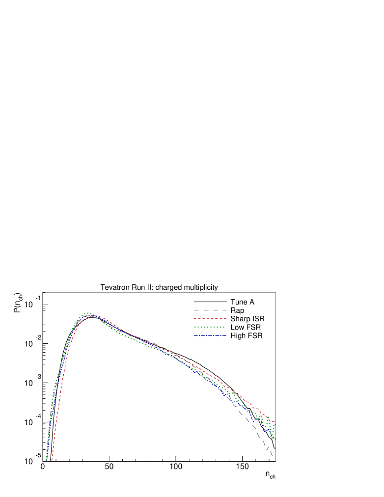
Figure 5: Charged multiplicity distributions, for 1.96 TeV $\mathrm{p}\overline{\mathrm{p}}$ minimum-bias events.

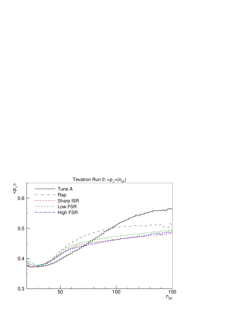
Figure 6: Average $p_{\perp}$ as a function of charged multiplicity, $\langle p_{\perp}\rangle(n_{\mathrm{ch}})$, for 1.96 TeV $\mathrm{p}\overline{\mathrm{p}}$ minimum-bias events. Note that the origo of the plot is not at (0,0).

While the multiplicity distributions have been brought into fair agreement with each other, the Tune A $\langle p_{\perp}\rangle(n_{\mathrm{ch}})$ is very difficult to duplicate in the new framework. This problem was also present for the models presented in [1]. Our interpretation is that this particular distribution is highly sensitive to the colour correlations, and we have so far been unsuccessful in identifying a physics mechanism that could explain the rather extreme correlations that are present in Tune A. Since data seems to be in fair agreement with Tune A here, the bottom line is that some kind of more or less soft colour correlations working between the scattering chains is likely to be present, beyond what our primitive fudge parameters $F$ and $F^{\prime}$ are capable of describing at this point.

4.2 Event activity

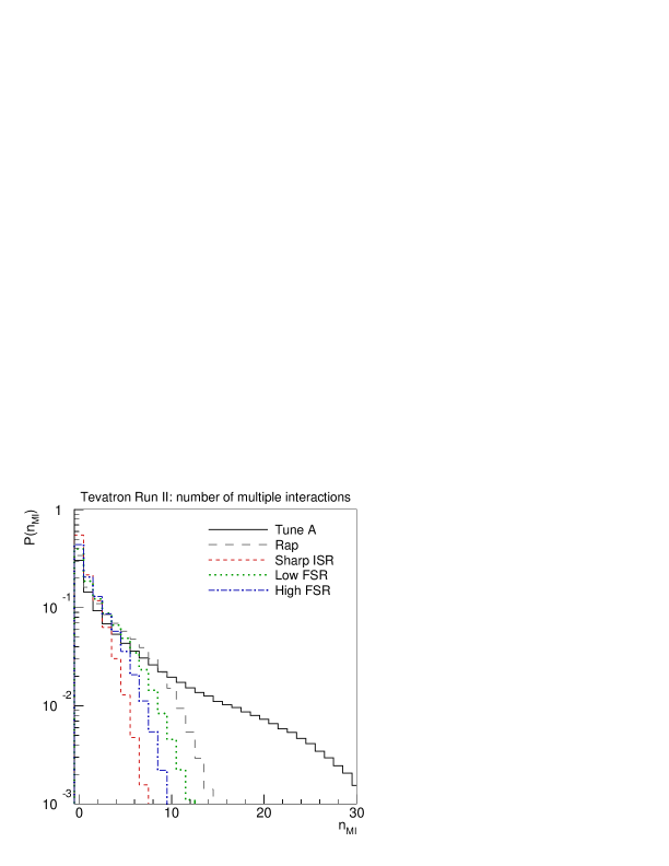
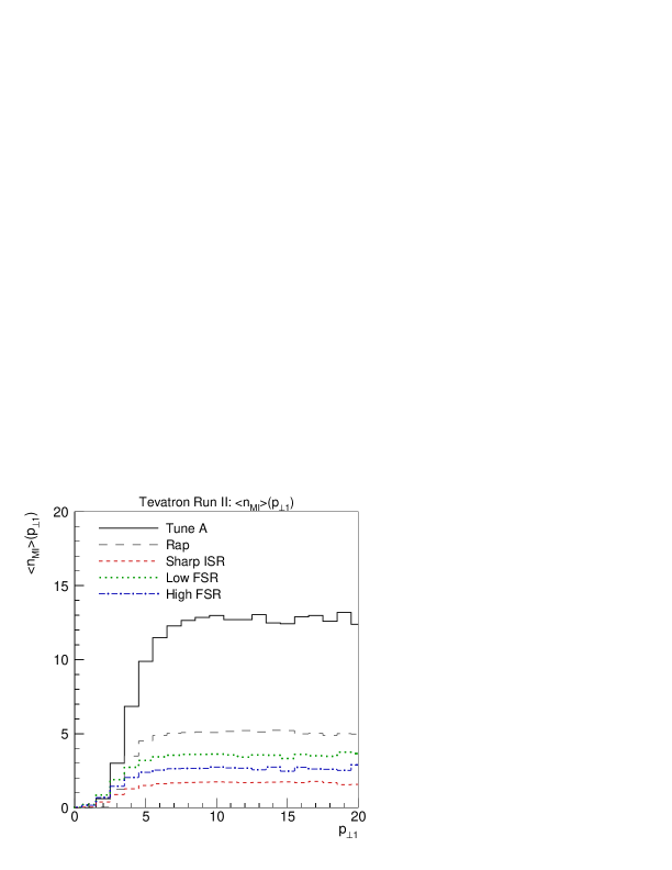
a)	b)

Figure 7: a) Number of multiple interactions (in addition to the hardest one) and b) the average number of additional interactions as a function of the $p_{\perp}$ of the hardest interaction, both for 1.96 TeV $\mathrm{p}\overline{\mathrm{p}}$ minimum-bias events.

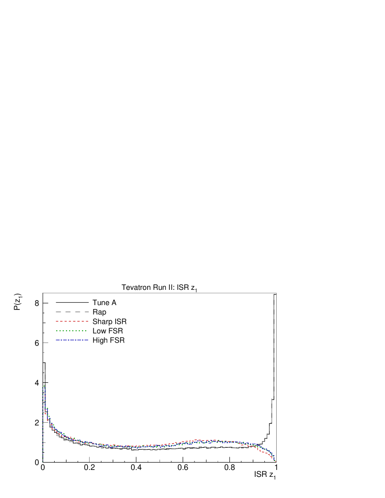
Figure 8: $z$ distributions for the first ISR branching, $z_{1}$, in 1.96 TeV $\mathrm{p}\overline{\mathrm{p}}$ minimum-bias events.

We now take a closer look at the relative proportions of the MI, ISR, and FSR make-up of minimum-bias events, for the models in Table 1. Firstly, the number of multiple interactions (excluding the hardest) is shown in Fig. 7a, and the dependence of the average number of extra interactions on the $p_{\perp}$ of the hardest interaction in Fig. 7b. The relatively low $p_{\perp 0}$ and slightly more peaked matter distribution of Tune A gives a tail towards very large multiplicities which is substantially reduced both in the new models and in the Rap tune. Surprisingly, the Low FSR scenario lies somewhat below the Rap model, even though the latter has a higher $p_{\perp 0}$ scale. A sanity check is to switch off ISR and then compare the four models with the same matter overlap. Without the ISR evolution competing for phase space, the $n_{\mathrm{MI}}$ distribution then looks as would be expected, with the lower $p_{\perp 0}$ scenario exhibiting the broadest distribution. Thus, the ISR branchings ‘eat up’ phase space more quickly in the new framework than before, leaving less room for multiple interactions. This conclusion is verified in Fig. 8, which compares the distribution of $z$ values for the first, i.e. hardest, ISR branching in an event. The soft-gluon enhancement of ISR near $z=1$ in the old models is absent in the new ones! This comes from the use of an evolution variable $p^{2}_{\perp\mathrm{evol}}=(1-z)Q^{2}$ in the latter ones, which favours larger $1-z$ in a branching than an evolution in $Q^{2}$, cf. the $z_{\mathrm{max}}$ expression in eq. (30).

In analogy with Fig. 7, the multiplicities of ISR and FSR branchings are depicted in Figs. 9 and 10, respectively. For ISR as well as for FSR, Tune A has by far the narrowest distributions, since only the hardest interactions are associated with parton showers. Concentrating on the ISR distribution, Fig. 9, again the Rap model exhibits a very broad distribution, together with the Sharp ISR model. This behaviour is characteristic of the threshold regularization of the ISR cascade employed in these models, which gives a larger number of fairly soft emissions than the smoothly regularized models, Low and High FSR. Also note that the smaller number of branchings in these models partly is compensated by the larger $\langle 1-z\rangle$ for the branchings that do occur.

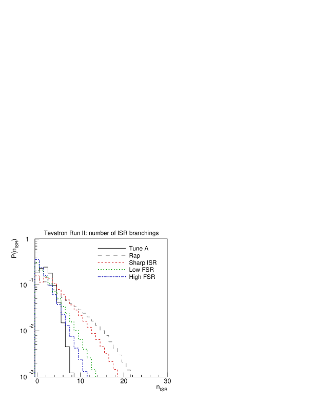
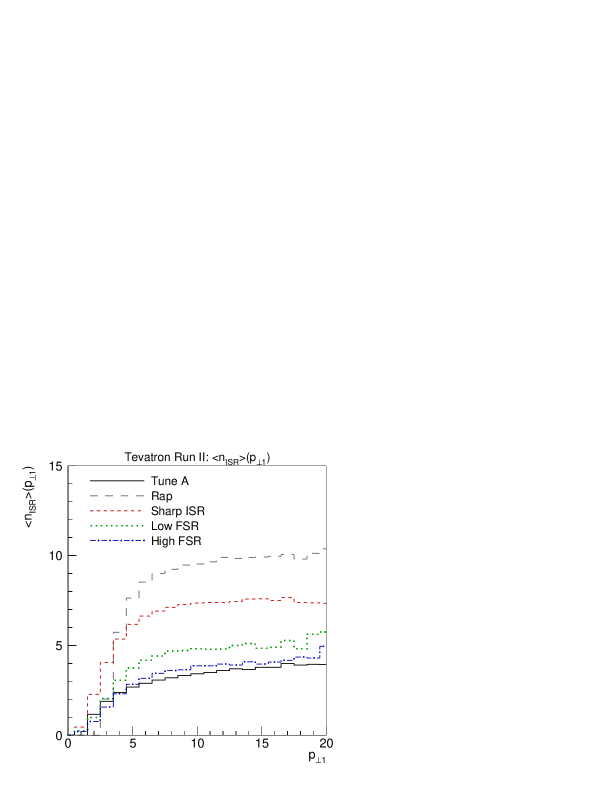
a)	b)

Figure 9: a) Number of ISR branchings and b) the average number of ISR branchings as a function of the $p_{\perp}$ of the hardest interaction, both for 1.96 TeV $\mathrm{p}\overline{\mathrm{p}}$ minimum-bias events.

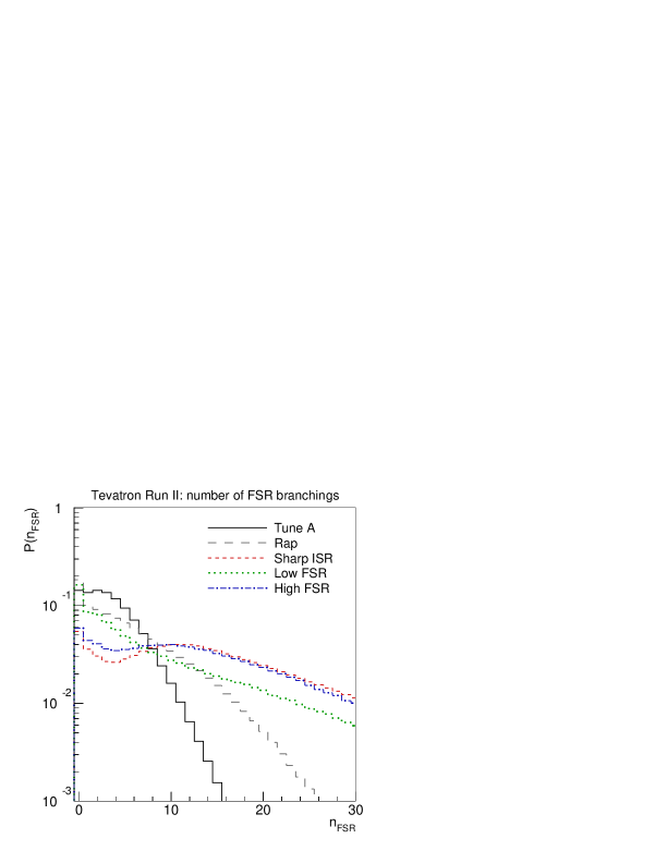
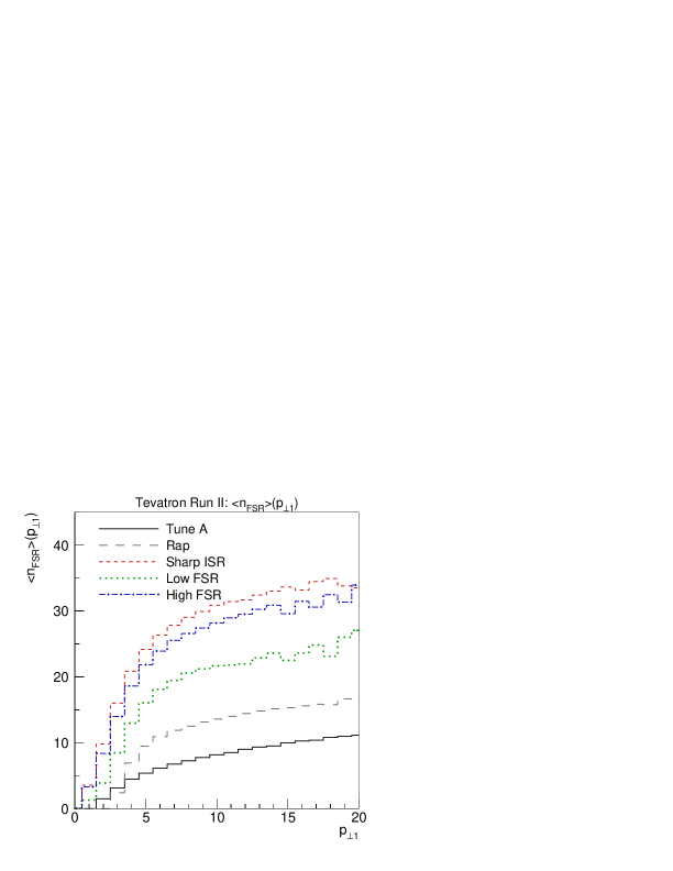
a)	b)

b)

Figure 10: Number of FSR branchings and b) the average number of FSR branchings as a function of the $p_{\perp}$ of the hardest interaction, both for 1.96 TeV $\mathrm{p}\overline{\mathrm{p}}$ minimum-bias events.

The large number of FSR branchings, Fig. 10, is related to the use of a very small cutoff here, of the order of $p_{\perp\mathrm{min}}=0.5$ GeV, and so it cannot be compared directly with the MI and ISR multiplicities. The new models clearly have much broader FSR distributions than both Tune A and the Rap model. As one would expect from the choice of maximum scale of emission, the Low FSR model is the narrowest of the new models. We also recall that there is a built-in compensation mechanism: if the number of ISR branchings is reduced then, other things being the same, this results in fewer but larger dipoles that therefore can radiate more. Although the old and new shower algorithms do not allow a straightforward comparison, the difference between Rap and the new models is at least consistent with such a partial compensation.

Returning now to observable distributions, the fact that less $p_{\perp}$ is kicked into events with large multiplicities in the new frameworks, cf. Fig. 6, while the multiplicity distributions are similar, also implies that there should be fewer events with large total $E_{\perp}$ than in Tune A. This is corroborated by Fig. 11, which shows the scalar sum of hadron $p_{\perp}$ values in 1.9  TeV $\mathrm{p}\overline{\mathrm{p}}$ minimum-bias events. Both the new models and the Rap model have noticeably fewer events in the region above $\sim 100$ GeV than does Tune A.

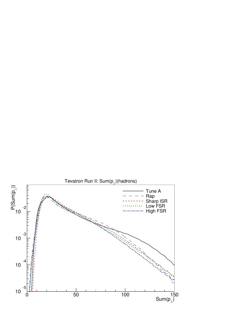
Figure 11: Total $p_{\perp}$ sum for hadrons in 1.96 TeV $\mathrm{p}\overline{\mathrm{p}}$ minimum-bias events.

In addition, Fig. 12 shows that the pseudorapidity distribution has become narrower, i.e. the particle production has become more central. The normalization differences are in this context not very interesting, arising from small differences in the average charged multiplicity of the tunes.

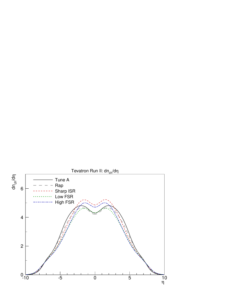
Figure 12: Charged multiplicity as a function of pseudorapidity $\eta$ in 1.96 TeV $\mathrm{p}\overline{\mathrm{p}}$ minimum-bias events.

However, these difference do not have a large impact on most other observables. Thus e.g. the minijet rates and charged hadron $p_{\perp}$ distributions in Figs. 13 and 14 are hardly distinguishable between Tune A and the new models. The minijet $E_{\perp}$ spectrum, defined by a simple cone algorithm with a cone radius of $R=\sqrt{(\Delta\eta)^{2}+(\Delta\phi)^{2}}=0.7$ and an $E_{\perp\mathrm{min}}=5$ GeV, which was slightly softer in the Rap model than in Tune A, has become slightly harder. On the other hand, the charged hadron $p_{\perp}$ spectrum, which was slightly harder in the Rap model than in Tune A, has dropped back down fairly close to the Tune A level.

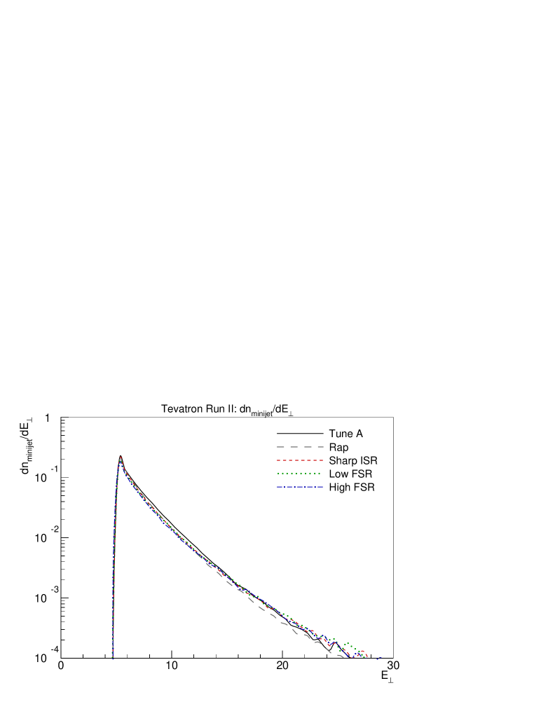
Figure 13: Minijet rates, for 1.96 TeV $\mathrm{p}\overline{\mathrm{p}}$ minimum-bias events.

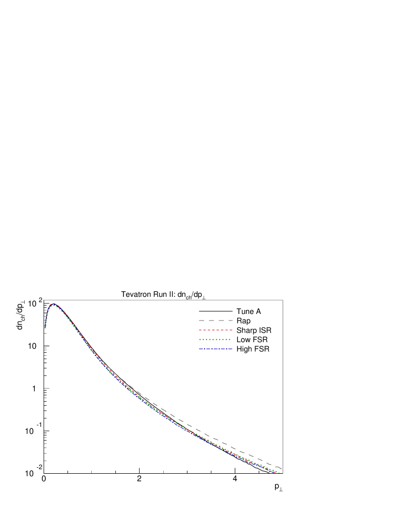
Figure 14: Charged hadron $p_{\perp}$ spectra in 1.96 TeV $\mathrm{p}\overline{\mathrm{p}}$ minimum-bias events. The normalization corresponds the total average charged multiplicity.

4.3 Jet events and profiles

Figure 15: Charged multiplicity distribution for 1.96 TeV $\mathrm{p}\overline{\mathrm{p}}$ events with $p_{\perp\mathrm{hard}}>100$ GeV.

Figure 16: Pseudorapidity distribution for 1.96 TeV $\mathrm{p}\overline{\mathrm{p}}$ events with $p_{\perp\mathrm{hard}}>100$ GeV.

Figure 17: Jet multiplicity distribution for 1.96 TeV $\mathrm{p}\overline{\mathrm{p}}$ events with $p_{\perp\mathrm{hard}}>100$ GeV, using a cone clustering algorithm with $R=0.7$ and $E_{\perp\mathrm{min}}=10$ GeV.

Figure 18: $E_{\perp}$ spectra for the hardest and third hardest jet in 1.96 TeV $\mathrm{p}\overline{\mathrm{p}}$ events with $p_{\perp\mathrm{hard}}>100$ GeV.

                                   a)                                                                     b)

Figure 19: The a) hardest and b) third hardest jet $E_{\perp}$ profile for 1.96 TeV $\mathrm{p}\overline{\mathrm{p}}$ events with $p_{\perp\mathrm{hard}}>100$ GeV.

                                   a)                                                                     b)

Figure 20: The a) charged multiplicity distribution and b) charged particle profile of the hardest jet in 1.96 TeV $\mathrm{p}\overline{\mathrm{p}}$ events with $p_{\perp\mathrm{hard}}>100$ GeV.

Complementary to the above are studies of events with hard jets and their properties. As an example of this, we have considered 1.96 TeV $\mathrm{p}\overline{\mathrm{p}}$ events where the hardest $2\to 2$ interaction has a $p_{\perp\mathrm{hard}}>100$ GeV, without any further requirements. The charged multiplicity distribution of such events is shown in Fig. 15, and their pseudorapidity distribution in Fig. 16. Given that the models have been tuned to each other exclusively for a minimum-bias event sample, the differences are less than could have been expected. We note a clear difference at mid-rapidities, however, where Tune A shows more activity than any of the newer scenarios, cf. also Fig. 12. This is likely to be related to the way strings are connected from the central interactions to the beam remnants.

The jet multiplicity in these events, obtained by a combination of MI, ISR and FSR activity, is shown in Fig. 17. The Low FSR scenario stands out by having significantly less jet activity than any of the other ones, clearly indicating the impact of the reduced FSR in these events. The other rates come surprisingly close, given that both the ISR and the FSR algorithms are quite different between the old and the new scenarios. At high jet multiplicities the new ones are somewhat above the older ones.

Next we study the properties of the jets produced. Since the two hardest jets both arise already as a consequence of the hard interaction, they have similar properties, while further jets are related to the additional activity and thus internally similar. Therefore only results for the hardest and (when present) third hardest jet are shown here. The respective jet $E_{\perp}$ spectra are shown in Fig. 18. The hardest jet is harder in all the three new scenarios than in the two old ones, while the third and subsequent ones are more similar. Again, given the changed ISR and FSR algorithms, the similarities for the third jet are more surprising than the differences for the first. Notably, the lower jet activity in the Low FSR scenario is not reflected in a reduced tail out to high-$E_{\perp}$ third jets.

The energy flow inside a jet can be plotted as a function of the distance $r$ away from the center of the jet, or better as a function of $r/R$. Such profiles are shown for the hardest and third jet in Fig. 19. For the hardest jet, again Low FSR stand out by producing narrower jets, while for the third Rap is even more narrow. Generally, the differences are small, however.

Turning to charged multiplicity distributions inside jets, the Rap scenario tends to have the least, and the High FSR and Sharp ISR the most. This is illustrated in Fig. 20a for the hardest jet, but the same pattern repeats also for the softer one. Comparing with the total charged multiplicity of these events, Fig. 15 above, which does not show the same pattern,we conclude that the balance between activity inside and outside the identified jets differs, possibly reflecting the amount of softer jet activity.

By contrast, the charged particle number jet profile follows the same pattern as observed above for the $E_{\perp}$ profile. That is, Low FSR gives the most narrow hardest jet, Fig. 20b, while Rap gives the most narrow third jet, not shown.

In summary, differences are smaller than might have been guessed, considering the changes especially in the ISR and FSR algorithms. Specifically, with the new algorithms the upper scale $p_{\perp\mathrm{max}}$ for ISR and FSR evolution is unambiguously set by the $p_{\perp\mathrm{hard}}$ of the hard interaction, while the older ones did involve an ambiguous choice of a $Q^{2}_{\mathrm{max}}=4p_{\perp\mathrm{hard}}^{2}$, intended roughly to give $p_{\perp}$ ordering, but not in the guaranteed sense of the new algorithms.

4.4 $\mathrm{Z}^{0}$ production

                                                                a)

                                                                b)

Figure 21: The $p_{\perp}$ spectrum at a) low and b) all $p_{\perp}$ for dilepton pairs in the 66–116 GeV mass range, $\gamma^{*}/\mathrm{Z}^{0}$ simulation compared with CDF corrected data at 1.8 TeV [35].

A slightly different test is to study the $p_{\perp}$ spectrum of high-mass dileptons coming from the decay of a $\gamma^{*}/\mathrm{Z}^{0}$. We can here compare with the CDF $p_{\perp\mathrm{Z}}$ spectrum at 1.8 TeV [35], normalizing the curves to the experimental integrated cross section, Fig. 21.

Since the high-$p_{\perp\mathrm{Z}}$ behaviour is constrained by our use of first-order matrix-element corrections [31], it is not surprising that differences here are small. That the three new scenarios are above the two older ones presumably is a consequence of the different treatment of FSR, which does not at all influence $p_{\perp\mathrm{Z}}$ in the new models, while the $p_{\perp}$ of an ISR branching is reduced by FSR in the older ones. This is a degree of freedom that could be studied further when FSR is interleaved with MI and ISR.

More interesting is the improvement in the low-$p_{\perp}$ region, similarly to what has been found earlier [32], in a study of the new ISR algorithm without any MI. However, note that we in all cases make use of a Gaussian primordial $k_{\perp}$ with a 2 GeV width (thus deviating from the pure Tune A, where it is kept at the Pythia default of 1 GeV). The implementation of this $k_{\perp}$ is more complex with the new beam-remnant implementation of [1], and e.g. could depend on the number of multiple interactions, but actually the distributions turn out to be quite similar. The problem therefore remains that this primordial $k_{\perp}$ is larger than can physically be well motivated based on purely nonperturbative physics. We observe that, among the new models, the Sharp ISR could have been combined with a smaller primordial $k_{\perp}$ since its peak is shifted towards too large $p_{\perp\mathrm{Z}}$, while the High FSR and Low FSR (which here only differ by their $p_{\perp 0}$ values) could have used an even larger primordial $k_{\perp}$. In part, this makes sense: with ISR being turned off at larger $p_{\perp}$ values in the latter models, it is then also easier to motivate a larger primordial $k_{\perp}$.

The complete comparison of algorithms is rather complicated, however. The primordial $k_{\perp}$ that reaches the hard interaction is diluted by the ISR activity, and so scales down like the ratio of the $x$ value of the incoming parton at the hard interaction to that of the initiator, $z_{\mathrm{tot}}=x_{\mathrm{in}}/x_{\mathrm{init}}$. This ratio is approximately the same for the old ISR shower ($\langle z_{\mathrm{tot}}\rangle\approx 0.59$) and Sharp ISR ($\langle z_{\mathrm{tot}}\rangle\approx 0.62$), indicating that the fewer ISR branchings and smaller $z$ per branching in the new algorithm rather well cancel. The smooth turnoff of High and Low FSR gives less branchings ($\langle z_{\mathrm{tot}}\rangle\approx 0.75$) and thus more primordial $k_{\perp}$ survives in these scenarios.

In summary, the new MI+ISR scheme gives an improved description of $\mathrm{Z}^{0}$ production, but does not remove the need for an uncomfortably large primordial $k_{\perp}$.

5 Outlook

In this article we have considered the consequences of interleaved multiple interactions and initial-state radiation, and paved the way for interleaving also final-state radiation in this framework, but that does not exhaust the list of perturbative processes in ‘normal’ hadronic events. One further possibility is that a parton from one of the incoming hadrons scatters twice, against two different partons from the other hadron, rescattering or ‘$3\to 3$’. Another possibility is that two partons participating in two separate hard scatterings may turn out to have a common ancestor when the backwards evolution traces the prehistory to the hard interactions, joined interactions (JI).

The $3\to 3$ processes have been considered in the literature [36], with the conclusion that they should be less important than multiple $2\to 2$ processes, except possibly at large $p_{\perp}$ values, where QCD radiation anyway is expected to be the dominant source of multijet events. The reason is that one $3\to 3$ scattering and two $2\to 2$ ones have similar parton-level cross sections, but the latter wins by involving one parton density more. Nevertheless, at some point, there ought to be a more detailed modelling, in order better to quantify effects.

The joined interactions are well-known in the context of the evolution of multiparton densities [37], but have not been applied to a multiple interactions framework. We will therefore here carry out a first study, to quantify roughly how common JI are and how much activity they contribute with. A full implementation of the complete kinematics, intertwining MI, ISR and JI all possible ways, is a major undertaking, worth the effort only if the expected effects are non-negligible. Given the many uncertainties in all the other processes at play, one would otherwise expect that the general tuning of MI/ISR/FSR/…to data would hide the effects of JI, as well as of $3\to 3$ processes.

5.1 Joined interactions: theory

Figure 22: Illustration of the three terms in the two-parton density evolution, eq. (46).

Just like the starting point for a discussion of ISR is the DGLAP evolution equations for the single-parton densities, the starting point for JI is the evolution equations for the two-parton densities. Relevant forwards-evolution formulae are available in the literature in integrated form [37]. Here, however, we will choose a differential form, that can then be applied to our backwards evolution framework. To this end, define the two-parton density $f^{(2)}_{bc}(x_{b},x_{c},Q^{2})$ as the probability to have a parton $b$ at energy fraction $x_{b}$ and a parton $c$ at energy fraction $x_{c}$ when the proton is probed at a scale $Q^{2}$. The evolution equation for this distribution is

$$\mathrm{d}f^{(2)}_{bc}(x_{b},x_{c},Q^{2}) = \frac{\mathrm{d}Q^{2}}{Q^{2}}\,\frac{\alpha_{\mathrm{s}}}{2\pi}\int\!\!\!\int\mathrm{d}x_{a}\,\mathrm{d}z\,\left\{\,f^{(2)}_{ac}(x_{a},x_{c},Q^{2})\,P_{a\to bd}(z)\,\delta(x_{b}-zx_{a})\right.$$ (46)

$$+\left.f^{(2)}_{ba}(x_{b},x_{a},Q^{2})\,P_{a\to cd}(z)\,\delta(x_{c}-zx_{a})\right.$$

$$+\left.f_{a}(x_{a},Q^{2})\,P_{a\to bc}(z)\,\delta(x_{b}-zx_{a})\,\delta(x_{c}-(1-z)x_{a})\right\}~{}.$$

As usual, we assume implicit summation over the allowed flavour combinations; thus the last term is absent when there is no suitable mother $a$ for a given set of $b$ and $c$. An illustration of the three terms is given in Fig. 22. The first two are the standard ones, where $b$ and $c$ evolve independently, up to flavour and momentum conservation constraints, and are already taken into account in the ISR framework. It is the last term that describes the new possibility of two evolution chains having a common ancestry.

Carrying out the $\delta$ integrations, which imply that $x_{a}=x_{b}+x_{c}$ and $z=x_{b}/(x_{b}+x_{c})$, the probability for the unresolution of $b$ and $c$ into $a$ when $Q^{2}$ is decreased (cf. the step from eq. (6) to eq. (7)) can be rewritten as

$$\mathrm{d}\mathcal{P}_{bc}(x_{b},x_{c},Q^{2}) = \left|\frac{\mathrm{d}f^{(2)}_{bc}(x_{b},x_{c},Q^{2})}{f^{(2)}_{bc}(x_{b},x_{c},Q^{2})}\right|\,$$ (47)

$$= \left|\frac{\mathrm{d}Q^{2}}{Q^{2}}\right|\,\frac{\alpha_{\mathrm{s}}}{2\pi}\,\frac{f_{a}(x_{a},Q^{2})}{f^{(2)}_{bc}(x_{b},x_{c},Q^{2})}\,\frac{1}{x_{b}+x_{c}}\,P_{a\to bc}(z)$$

$$= \left|\frac{\mathrm{d}Q^{2}}{Q^{2}}\right|\,\frac{\alpha_{\mathrm{s}}}{2\pi}\,\frac{x_{a}f_{a}(x_{a},Q^{2})}{x_{b}x_{c}f^{(2)}_{bc}(x_{b},x_{c},Q^{2})}\,z(1-z)P_{a\to bc}(z)$$

$$\simeq \left|\frac{\mathrm{d}Q^{2}}{Q^{2}}\right|\,\frac{\alpha_{\mathrm{s}}}{2\pi}\ \frac{x_{a}f_{a}(x_{a},Q^{2})}{x_{b}f_{b}(x_{b},Q^{2})\,x_{c}f_{c}(x_{c},Q^{2})}\,z(1-z)P_{a\to bc}(z)~{}.$$

In the last step we have introduced the approximation $f^{(2)}_{bc}(x_{b},x_{c},Q^{2})\simeq f_{b}(x_{b},Q^{2})\,f_{c}(x_{c},Q^{2})$ to put the equation in terms of more familiar quantities. Just like for the other processes considered, a form factor is given by integration over the relevant $Q^{2}$ range and exponentiation.

The strategy now is clear. Previously we have introduced a scheme wherein events are evolved downwards in $p_{\perp}$. At each step a new trial multiple interaction competes against trial ISR branchings on the existing interactions, and the one with largest $p_{\perp}$ ‘wins’. Now a third option is added, competing with the first two in the same way, i.e. eq. (45) is extended to

$$\frac{\mathrm{d}\mathcal{P}}{\mathrm{d}p_{\perp}} = \left(\frac{\mathrm{d}\mathcal{P}_{\mathrm{MI}}}{\mathrm{d}p_{\perp}}+\sum\frac{\mathrm{d}\mathcal{P}_{\mathrm{ISR}}}{\mathrm{d}p_{\perp}}+\sum\frac{\mathrm{d}\mathcal{P}_{\mathrm{JI}}}{\mathrm{d}p_{\perp}}\right)\;\times$$ (48)

$$\times\;\exp\left(-\int_{p_{\perp}}^{p_{\perp i-1}}\left(\frac{\mathrm{d}\mathcal{P}_{\mathrm{MI}}}{\mathrm{d}p_{\perp}^{\prime}}+\sum\frac{\mathrm{d}\mathcal{P}_{\mathrm{ISR}}}{\mathrm{d}p_{\perp}^{\prime}}+\sum\frac{\mathrm{d}\mathcal{P}_{\mathrm{JI}}}{\mathrm{d}p_{\perp}^{\prime}}\right)\mathrm{d}p_{\perp}^{\prime}\right)~{}.$$

The JI sum runs over all pairs of initiator partons with allowable flavour combinations, separately for the two incoming hadrons. A gluon line can always be joined with a quark or another gluon one, and a sea quark and its companion can be joined into a gluon. For each of these possibilities, $\mathrm{d}\mathcal{P}_{\mathrm{JI}}\,\exp(-\int\mathrm{d}\mathcal{P}_{\mathrm{JI}})$ can be used to do a backwards evolution from the $p_{\perp\mathrm{max}}=p_{\perp i-1}$ scale given by the previous step. If such a trial joining occurs at a larger $p_{\perp}$ scale than any of the other trial possibilities, then it is allowed to occur. Also the regularization procedure at small $p_{\perp}$ values is the same as for MI and ISR.

The parton densities we will use are defined in the same spirit as previously discussed, e.g. $f_{b}(x_{b},p^{2}_{\perp})$ and $f_{c}(x_{c},p^{2}_{\perp})$ are squeezed into ranges $x\in[0,X]$, where $X$ is reduced from unity by the momentum carried away by all but the own interaction, and for $f_{a}(x_{a},p^{2}_{\perp})$ by all but the $b$ and $c$ interactions. Note that companion distributions are normalized to unity. Therefore, for heavy quarks, the branching probability $\mathrm{g}\to\mathrm{Q}\overline{\mathrm{Q}}$ goes like $1/\ln(p^{2}_{\perp}/m_{\mathrm{Q}}^{2})$ for $p^{2}_{\perp}\to m_{\mathrm{Q}}^{2}$, as it should, rather than like $1/\ln^{2}(p^{2}_{\perp}/m_{\mathrm{Q}}^{2})$, which would have been obtained if $f_{\mathrm{Q}}$ and $f_{\overline{\mathrm{Q}}}$ independently were assumed to vanish in this limit.

Figure 23: Kinematics of the $b+d$ and $c+e$ colliding systems (a) before and (b) after the $a\to b+c$ branching is reconstructed.

Unfortunately the kinematics reconstruction offers a complication. Consider a system with recoilers $d$ and $e$ to $b$ and $c$, respectively, as depicted in Fig. 23. Use a prime to denote the modified $b$ and $c$ four-momenta after the $a\to b+c$ branching has been constructed, while $d$ and $e$ should be unchanged. From $x_{a}=x_{b}+x_{c}$ it then follows that $p_{a}=p_{b}+p_{c}=p^{\prime}_{b}+p^{\prime}_{c}$, and from the $z$ definition that

$$(p^{\prime}_{b}+p_{d})^{2}=(p_{b}+p_{d})^{2} = z(p_{a}+p_{d})^{2}~{},$$ (49)

$$(p^{\prime}_{c}+p_{e})^{2}=(p_{c}+p_{e})^{2} = (1-z)(p_{a}+p_{e})^{2}~{}.$$ (50)

Further, $p^{\prime}_{b}$ and $p^{\prime}_{c}$ should have opposite and compensating transverse momenta given by the $p_{\perp}$ scale above, and spacelike virtualities to be determined. Now, it turns out that these requirements overconstrain the system. The basic problem is illustrated by eq. (27): the spacelike parton needs to pick up a larger $p_{\parallel}$ component than its $z$ share, in order to retain the invariant mass with the recoiler when the $p_{\perp}$ is introduced. So, if both daughters should be spacelike, not both of them can pick up more $p_{\parallel}$ than $E$, given that $a$ is massless. (A solution where one of $p^{\prime}_{b}$ and $p^{\prime}_{c}$ is timelike sometimes exists, but not always, and is anyway rather contrived.)

We see two alternative ways out of this dilemma.

• Retain the $x_{a}=x_{b}+x_{c}$ expression, at the expense of not giving any $p_{\perp}$ or virtualities in the branching, i.e. $p^{\prime}_{b}=p_{b}$ and $p^{\prime}_{c}=p_{c}$. Then $p_{\perp}$ only plays the role of a formal evolution parameter, denoting the scale above which $b$ and $c$ may radiate and interact separately.

• Insist on having a $p_{\perp}$ kick in the branching. Then a sensible (but not unique) choice is to put ${p^{\prime}_{b}}^{2}={p^{\prime}_{c}}^{2}=-p_{\perp}^{2}$, such that both have $m_{\perp}=0$ and thus $p_{\parallel}=E$. These energies must now be scaled up somewhat, to $E^{\prime}_{b}=(1+p^{2}_{\perp}/m_{bd}^{2})E_{b}$ and $E^{\prime}_{c}=(1+p^{2}_{\perp}/m_{ce}^{2})E_{c}$, for the invariant masses with the recoiler to be preserved, and therefore

  $$x_{a}=\left(1+\frac{p^{2}_{\perp}}{m_{bd}^{2}}\right)x_{b}+\left(1+\frac{p^{2}_{\perp}}{m_{ce}^{2}}\right)x_{c}~{}.$$ (51)

  It is then this $x_{a}$ that should be used in parton densities, to ensure that the probability of a joining is suppressed near the kinematical limit.

Given that no joinings are possible until after (at least) two interactions have been generated, and that the rate increases roughly quadratically with the number of interactions, this physics mechanism becomes more important at smaller $p_{\perp}$ values. Therefore we do not expect the above two extremes to differ that significantly for practical applications.

5.2 Joined interactions: results

Although an algorithm implementing the full kinematics for joined interactions has not yet been constructed, it is still possible to gauge the order of magnitude of the effects such joinings could have. We do this by formally performing the backwards evolution according to eq. (48), i.e. including the joining term eq. (47) in competition with the ordinary ISR and MI terms, without actually letting the generated joinings occur physically. Thereby we still obtain an estimate for how often and at which $p_{\perp}$ values joinings would occur.

Since we do not perform the joinings physically, the backwards evolution could in principle attempt joinings involving the same initial state shower chain more than once. Such joinings are of course rejected; only the first joining involving a particular chain is kept track of.

Taking the High FSR model in Table 1 as a fair representative of the evolution in the new framework, we show the number distributions of multiple interactions excluding the first (MI), ISR branchings, FSR branchings, and trial joinings (JI) in 1.96 TeV $\mathrm{p}\overline{\mathrm{p}}$ minimum-bias events, Fig. 24a, and for events where the $p_{\perp}$ of the hard interaction is above 100 GeV, Fig. 24b. Below, we refer to the former as the “min-bias” sample and to the latter as the “UE” (underlying event) sample.

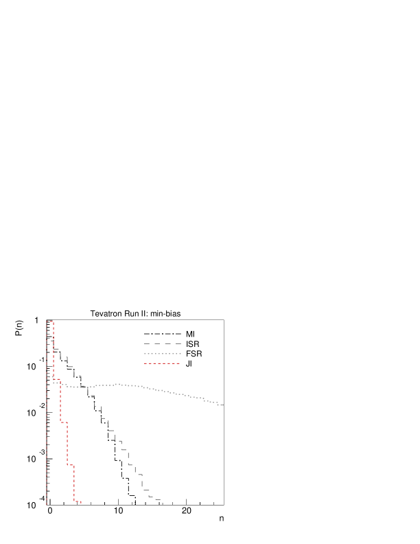
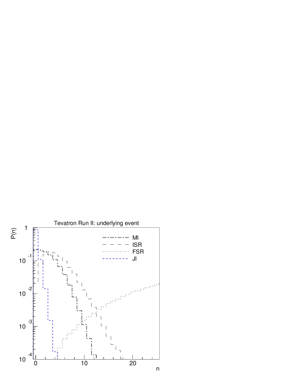
a)	b)

Figure 24: Probability distributions of MI, ISR, FSR, and JI in a) min-bias events and b) events with $p_{\perp\mathrm{hard}}>100$ GeV, for 1.96 TeV $\mathrm{p}\overline{\mathrm{p}}$ events. Note that the MI distribution does not include the hardest scattering.

FSR is shown mainly for reference here, the important graphs being the ones illustrating the evolution in the initial state: MI, ISR, and JI. One clearly observes that joinings are much less frequent than the other types of evolution steps, averaging at roughly one joining per 15 events for the min-bias sample and one per 7 events for the UE sample. Thus, even when relatively hard physics is involved, shower joinings do not appear to take a very prominent role in the evolution.

To complement the number distributions, Fig. 25 shows

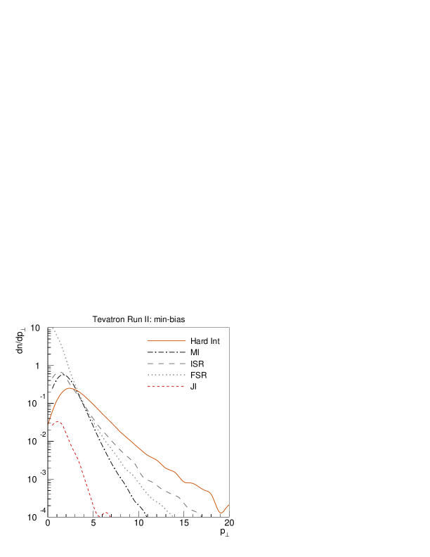
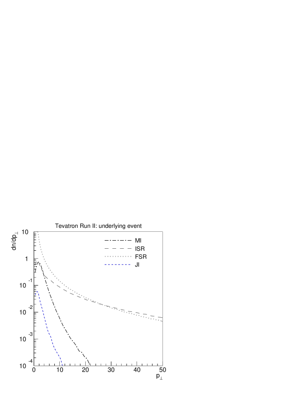
a)	b)

Figure 25: $p_{\perp\mathrm{evol}}$ distributions showing the scale at which multiple interactions (MI), ISR branchings, FSR branchings, and joined interactions (JI) occur, in 1.96 TeV $\mathrm{p}\overline{\mathrm{p}}$ min-bias events. a) Minimum-bias events, with the $p_{\perp}$ scale of the hardest interaction shown for reference (solid line). b) events with $p_{\perp\mathrm{hard}}>100$ GeV. Note that the $p_{\perp}$ axis goes out to 20 GeV in a) and to 50 GeV in b).

where the evolution steps occur in $p_{\perp\mathrm{evol}}$. As expected, the joinings occur at comparatively low values of $p_{\perp\mathrm{evol}}$. Also notice that both the ISR, MI, and JI distributions exhibit a turnover around $p_{\perp 0}$, characteristic of the smooth regularization used in the High FSR model.

Finally, Fig. 26 shows the total $p_{\perp}$ sum of MI, ISR, FSR, and JI activity, respectively. That is, for each interaction, branching, or joining, a scalar $p_{\perp}$ is defined, which is added to a cumulative sum. For MI and JI this $p_{\perp}$ is defined with respect to the beam axis, while the ISR and FSR $p_{\perp}$ is defined with respect to the branching parton, which for ISR is roughly along the beam direction, but for FSR normally not. Therefore FSR mainly broadens jets, i.e. redistributes the existing $E_{\perp}$, whereas the other mechanisms increase the total $E_{\perp}$ of the event.

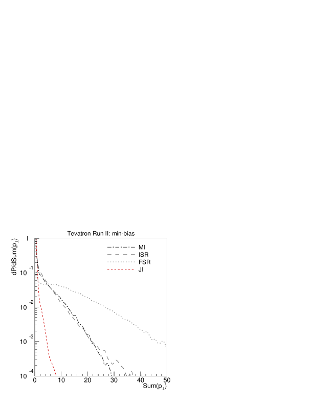
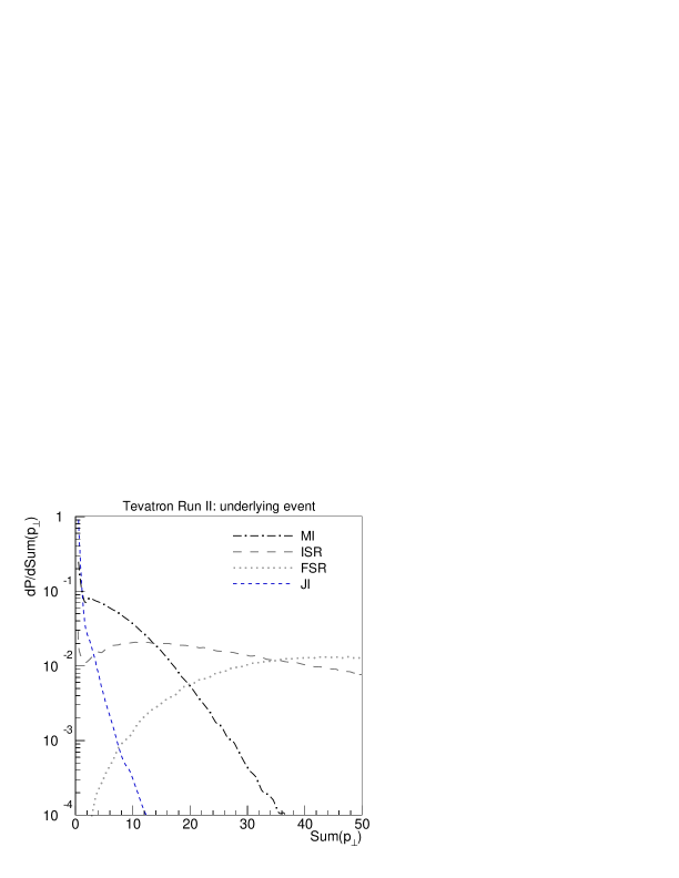
a)	b)

Figure 26: $\sum p_{\perp}$ distributions for MI, ISR, FSR and JI, in 1.96 TeV $\mathrm{p}\overline{\mathrm{p}}$ a) minimum-bias events and b) events with $p_{\perp\mathrm{hard}}>100$ GeV. Note that the MI distribution does not include the hardest scattering.

Again, the cumulative effect of joinings is small, with only about 1% of the min-bias sample and 5% of the UE one exhibiting more than 2 GeV of total $p_{\perp}$ from joinings.

6 Conclusions

It would seem natural to consider the evolution of a high-energy event in the normal time order. In such a framework, the incoming hadrons are evolved from a simple partonic configuration at a low $Q_{0}$ scale, up through a number of short-lived fluctuations at different virtuality scales. At the moment of collision, the two sets of partons may undergo several independent interactions. The scattered partons can radiate in the final state, while fluctuations inside which no scatterings occurred may recombine. Finally the set of outgoing low-virtuality partons hadronize.

Such an approach has the advantage that it inherently provides multiparton distributions, and thereby automatically contains correlations between interactions, including what is here called joined interactions. It does not remove the need to consider possible scatterings in some order of hardness, however: the partons of a high-virtuality fluctuation may either interact individually or collectively, the latter as the unresolved mother parton at a lower resolution scale, and the former should preempt the latter.

There is also the well-known problem that it is difficult to generate rare processes, since there is no straightforward way to preselect the forwards evolution to give the desired configuration. The nightmare example is the production of a narrow Higgs state, where the incoming partons must match very precisely in invariant mass for a reaction to be possible. More generally, efficiency suffers from the need to consider a wealth of virtual fluctuations that in the end lead to nothing. The assignment of individual virtualities and transverse momenta to partons in such fluctuations is also not unique, and does affect the kinematics reconstruction. And, of course, the whole plethora of coherence effects need to be considered.

The alternative is to start with the hardest interaction, and then ‘work outwards’ to longer timescales both in the past and future, i.e. to (re)construct less hard steps in the evolution of the event. This makes the preselection of desired events straightforward, and in general implies that the most striking aspects of the event are considered ‘up front’. The price is a tougher task of reconstructing the soft associated activity in the initial state, while final-state radiation and hadronization offer about the same challenges in the two scenarios.

In a set of articles we have begun the task of providing an improved description of events along this latter philosophy. The first step [3] was to develop a model for the hadronization of junction topologies, thereby allowing complicated beam remnants. The second step [1] was to develop a framework for correlated parton densities, in flavour, colour and transverse and longitudinal momentum, thereby allowing initial-state radiation to be considered in full. In this, the third step, we have interleaved multiple interactions and initial-state radiation in a common transverse-momentum-ordered sequence, with a common dampening procedure at low transverse momenta to handle destructive interference in this region. Our lack of explicitly implemented joined interactions has been shown not to be a major shortcoming, since such joinings are reasonably rare. That is, taken together, we now have a framework that should provide a complete description of all aspects that could have been covered by a forwards-in-time evolution scenario, along with the traditional advantages of the backwards-evolution approach. In addition, the new framework makes use of new algorithms for $p_{\perp}$-ordered evolution in initial- and final-state radiation, which should further improve the quality of the description.

It may then be somewhat disappointing that we here have used Pythia Tune A [34] as a reference, well knowing that Tune A is able to describe a host of jet and minimum-bias data at the Tevatron, in spite of it being based on a much more primitive approach [2]. The hope, of course, is that our new approach will be able to explain — and predict — much more data than Tune A can. For sure we know of many aspects of the old framework that are unreasonable, but that either have not been probed or that may have been fixed up by a contrived choice of tuned parameters. Ultimately this is for experimentalists to tell, as tests become increasingly more sophisticated. Certainly, one should not expect the advantages of the new model to become apparent unless a similar effort is mounted as went into producing Tune A in the first place.

There are also a few issues still hanging over us, awaiting a ‘fourth step’. One is the implementation of joined interactions and $3\to 3$ rescattering processes, to see what their real impact is, whether negligible or not. But the main one we believe to be the interleaving of final-state radiation with multiple interactions and initial-state radiation. On the one hand, such an interleaving may not be required, since the competition between FSR and MI+ISR is less direct than that between MI and ISR: an FSR emission at a high $p_{\perp}$ scale does not affect the probability for MI or ISR activity at lower $p_{\perp}$ values. On the other hand, there would then also not seem to be any disadvantage to having a commonly ordered $p_{\perp}$ sequence of MI+ISR+FSR, and such an ordering would come in handy for a consistent interfacing to higher-order matrix elements. Furthermore, a $p_{\perp}$-ordered FSR algorithm is available, well matched to the $p_{\perp}$-ordering of MI and ISR.

There is, however, one major open question related to FSR interleaving: which parton takes the momentum recoil when a FSR branching pushes a parton off the mass shell? The problem is not so much the momentum transfer itself, but that the size of the radiating dipole sets the maximum scale for allowed emissions. We have in this article illustrated how such a choice can affect e.g. the jet multiplicity and jet profiles. The crucial distribution is the $\langle p_{\perp}\rangle(n_{\mathrm{ch}})$ one, however. In order to provide a reasonable description of the experimental data, we are forced to arrange colours in the final state to have a smaller string length than colour correlations in the initial state alone would suggest. This problem has ‘always’ been there [2], and is accentuated in Tune A, where as much as 90% of the partons added by multiple interactions are connected so as to minimize the string length. The hope that an improved treatment of other aspects would remove the need for a special string-length minimization mechanism has so far failed to materialize. We therefore need to understand better how the colour flow is set, and how this influences the evolution of an event, especially the FSR activity.

The related fields of minimum bias physics and underlying events thus are further explored but not solved with this article, and likely not with the next one either. This should come as no surprise: in the world of hadronic physics, there are few simple answers. Everything that is not explicitly forbidden is bound to happen, and often at a significant rate. To reflect reality, the theoretical picture therefore has to become more and more complex, as one consideration after the next is pulled into the game. However, if the journey is interesting and educational, why despair that the end station is not yet reached?

Acknowledgements

We are grateful to G. Rudolph for having tuned our new $p_{\perp}$-ordered final-state shower algorithm to LEP data. Communications with Tevatron and LHC physicists, especially R.D. Field, J. Huston and A. Moraes, have spurred us on.

References

- [1] T. Sjöstrand and P.Z. Skands, JHEP 03 (2004) 053
- [2] T. Sjöstrand and M. van Zijl, Phys. Rev. D36 (1987) 2019
- [3] T. Sjöstrand and P.Z. Skands, Nucl. Phys. B659 (2003) 243
-
[4]
T. Sjöstrand, Phys. Lett. 157B (1985) 321;
M. Bengtsson, T. Sjöstrand and M. van Zijl, Z. Phys. C32 (1986) 67 - [5] T. Sjöstrand, LU TP 04–05 [hep-ph/0401061], in the QCD/SM Working Group Summary Report of the Physics at TeV Colliders Workshop, Les Houches, France, 26 May – 6 Jun 2003 [hep-ph/0403100]
-
[6]
T. Sjöstrand, P. Edén, C. Friberg, L. Lönnblad, G. Miu, S. Mrenna
and E. Norrbin, Computer Phys. Commun. 135 (2001) 238;
T. Sjöstrand, L. Lönnblad, S. Mrenna and P. Skands, LU TP 03-38 [hep-ph/0308153]. -
[7]
V.N. Gribov and L.N. Lipatov, Sov. J. Nucl. Phys. 15 (1972) 438,
ibid. 75;
G. Altarelli and G. Parisi, Nucl. Phys. B126 (1977) 298;
Yu.L. Dokshitzer, Sov. J. Phys. JETP 46 (1977) 641 -
[8]
B. Andersson, G. Gustafson, G. Ingelman and T. Sjöstrand,
Phys. Rep. 97 (1983) 31;
T. Sjöstrand, Nucl. Phys. B248 (1984) 469;
B. Andersson, ‘The Lund Model’ (Cambridge University Press, 1998) - [9] V.V. Sudakov, Zh.E.T.F. 30 (1956) 87 (Sov. Phys. J.E.T.P. 30 (1956) 65)
- [10] M. Bengtsson and T. Sjöstrand, Nucl. Phys. B289 (1987) 810
- [11] E. Norrbin and T. Sjöstrand, Nucl. Phys. B603 (2001) 297
-
[12]
G. Marchesini and B.R. Webber, Nucl. Phys. B238 (1984) 1;
G. Corcella, I.G. Knowles, G. Marchesini, S. Moretti, K. Odagiri, P. Richardson, M.H. Seymour and B.R. Webber, JHEP 01 (2001) 010, hep-ph/0210213 - [13] G. Gustafson, Phys. Lett. B175 (1986) 453
- [14] G. Gustafson and U. Pettersson, Nucl. Phys. B306 (1988) 746
- [15] L. Lönnblad, Computer Physics Commun. 71 (1992) 15
-
[16]
A.H. Mueller, Phys. Lett. 104B (1981) 161;
B.I. Ermolaev, V.S. Fadin, JETP Lett. 33 (1981) 269 - [17] M.H. Seymour, Computer Physics Commun. 90 (1995) 95
- [18] G. Gustafson, private communication
-
[19]
S. Catani, F. Krauss, R. Kuhn and B.R. Webber,
JHEP 11 (2001) 063;
L. Lönnblad, JHEP 05 (2002) 046 -
[20]
P. Skands and T. Sjöstrand, LU TP 03-45 [hep-ph/0310315], in the
proceedings of International Europhysics
Conference on High-Energy Physics (HEP 2003), Aachen, Germany, 17-23 Jul
2003, European Physical Journal C Direct, DOI:
10.1140/epjcd/s2003-03-520-7;
T. Sjöstrand and P. Skands, LU TP 04-04 [hep-ph/0401060], in The QCD/SM working group: Summary report, 3rd Les Houches Workshop: Physics at TeV Colliders, Les Houches, France, 26 May - 6 Jun 2003, M. Dobbs et al. [hep-ph/0403100] -
[21]
OPAL Collaboration, M.Z. Akrawy et al.,
Z. Phys. C47 (1990) 505;
L3 Collaboration, B. Adeva et al., Z. Phys. C55 (1992) 39;
I.G. Knowles et al., in ‘Physics at LEP2’, eds. G. Altarelli, T. Sjöstrand and F. Zwirner, CERN 96–01 (Geneva, 1996), Vol. 2, p. 103;
DELPHI Collaboration, P. Abreu et al., Z. Phys. C73 (1996) 11;
ALEPH Collaboration, R. Barate et al., Phys. Rep. 294 (1998) 1 -
[22]
B. Andersson et al., Eur. Phys. J. C25 (2002) 77;
J. Andersen et al., Eur. Phys. J. C35 (2004) 67 - [23] B. Andersson, G. Gustafson, L. Lönnblad and U. Pettersson, C. Phys. C43 (1989) 625
-
[24]
B. Andersson, G. Gustafson and J. Samuelsson,
Nucl. Phys. B467 (1996) 443;
B. Andersson, G. Gustafson and H. Kharraziha, Phys. Rev. D57 (1998) 5543;
H. Kharraziha and L. Lönnblad, JHEP 03 (1998) 006 -
[25]
M. Ciafaloni, Nucl. Phys. B296 (1987) 249;
S. Catani, F. Fiorani and G. Marchesini, Nucl. Phys. B336 (1990) 18 - [26] T. Sjöstrand, Computer Physics Commun. 28 (1983) 229
- [27] S. Catani, Yu. L. Dokshitzer, M. Olsson, G. Turnock and B.R. Webber, Phys. Lett. B269 (1991) 432
-
[28]
D. Amati, A. Bassetto, M. Ciafaloni, G. Marchesini and G. Veneziano,
Nucl. Phys. B173 (1980) 429;
G. Curci, W. Furmanski and R. Petronzio, Nucl. Phys. B175 (1980) 27 - [29] B.R. Webber, Ann. Rev. Nucl. Part. Sci. 36 (1986) 253
- [30] G. Rudolph, private communication
- [31] G. Miu and T. Sjöstrand, Phys. Lett. B449 (1999) 313
-
[32]
E. Thomé, master’s thesis, Lund University, LU TP 04–01
[hep-ph/0401121];
J. Huston, I. Puljak, T. Sjöstrand, E. Thomé, LU TP 04–07 [hep-ph/0401145], in the QCD/SM Working Group Summary Report of the Physics at TeV Colliders Workshop, Les Houches, France, 26 May – 6 Jun 2003 [hep-ph/0403100] -
[33]
A. Breakstone et al., Phys. Lett. 132B (1983) 463;
UA1 Collaboration, C. Albajar et al., Nucl. Phys. B335 (1990) 261;
E735 Collaboration, T. Alexopoulos et al., Phys. Lett. B336 (1994) 599;
CDF Collaboration, D. Acosta et al., Phys. Rev. D65 (2002) 072005 - [34] R.D. Field, presentations at the ‘Matrix Element and Monte Carlo Tuning Workshop’, Fermilab, 4 October 2002 and 29–30 April 2003, talks available from webpage http://cepa.fnal.gov/CPD/MCTuning/, and further recent talks available from http://www.phys.ufl.edu/rfield/cdf/
- [35] CDF Collaboration, T. Affolder et al., Phys. Rev. Lett. 84 (2000) 845
- [36] N. Paver and D. Treleani, Nuovo Cimento 70A (1982) 215, Phys. Lett. 146B (1984) 252, Z. Phys. C28 (1985) 187
-
[37]
K. Konishi, A. Ukawa and G. Veneziano,
Nucl. Phys. B157 (1979) 45;
R. Kirschner, Phys. Lett. 84B (1979) 266;
V.P. Shelest, A.M. Snigirev and G.M. Zinovjev, Phys. Lett. 113B (1982) 325;
A.M. Snigirev, Phys. Rev. D68 (2003) 114012;
V.L. Korotkikh and A.M. Snigirev, hep-ph/0404155