$B\to X_{s}\ell^{+}\ell^{-}$ and $B\to K\pi$ decays in vectorlike quark model

Abstract

In the framework of SU(2) singlet down type vectorlike quark model, we present a comprehensive analysis for decays $B\to X_{s}\gamma,\ B\to X_{s}l^{+}l^{-}$ and $B\to K\pi$. As for $B\to X_{s}\gamma$, we include the QCD running from the mass of the down-type vector quark $D$ to weak scale in the scenario with the D quark much heavier than weak scale, and find that the running effect is small. Using the recent measurements of $B\to X_{s}l^{+}l^{-}$, we extract rather stringent constraints on the size and CP violating phase of $z_{sb}$, i.e., the tree level FCNC coupling for $b\to sZ$. Within the bounds, we investigate various observables such as forward-backward asymmetry of $b\to sl^{+}l^{-}$, the decay rates of $B\to X_{s}\gamma$, and $B\to K\pi$. We find that (1) The forward-backward asymmetry may have large derivation from that of the SM and is very sensitive to $z_{sb}$, and thus can be useful in probing the new physics. (2) By taking experimental errors at $2\sigma$ level, both experimental measurements for $B\to X_{s}l^{+}l^{-}$ and $B\to K\pi$ decays can be explained in this model.

I Introduction

The study of flavor changing neutral currents (FCNC) in particle physics phenomenology has played a key role in advance of high energy physics in the past decades. Due to the GIM mechanism, FCNC in the standard model (SM) arises only at higher loop level, and thus, it makes FCNC phenomena a privileged ground to search for signs of new physics beyond the SM. However, in extension of the SM such as vector quark model (VQM), the CKM matrix is necessarily non-unitarity, leading to interaction $Z\bar{s}b$ at tree level, and hence potentially large new physics contributions can be expected.

The rare radiative decays $B\to X_{s}\gamma$ and $B\to X_{s}l^{+}l^{-}$ are sensitive probes of new physics [1]. The branching ratio of the radiative decay $B\to X_{s}\gamma$ has been measured by BaBar [2], CLEO[3], and ALEPH[4] and is in good agreement with the SM predictions [5, 6]. Recently, the rare decays $B\to X_{s}l^{+}l^{-}\ (l=e,\mu)$ also have been measured by BaBar[7] and Belle[8]. The average value is [9]

$${\cal B}r^{ex}(B\to X_{s}l^{+}l^{-})=\left(6.2\pm 1.1^{+1.6}_{-1.3}\right)\times 10^{-6}.$$ (1)

Although the process $B\to X_{s}\gamma$ constrains the parameters of the VQM [10, 11], since vectorlike down-type quark contributions to $b\to s\gamma$ just occur at loop level as the case of the SM, the constraints on $z_{sb}$, the tree level FCNC coupling for $b\to sZ$, from $B\to X_{s}\gamma$ are less restrictive compared to those from processes governed by $b\to sl^{+}l^{-}$ transition.

There are some studies regarding the constraints on model with extra singlet quark [10, 11, 12, 13]. In light of the improvement in the experimental data, it is necessary to present a comprehensive analysis in this model. Also, from the point of view of the model builder, it is important how the presence of the singlet quark may have impact on low energy phenomenology. In particular, mass of the singlet quark, the coupling to ordinary quarks and weak gauge bosons are very important issues. We extend the previous studies and take the following points of the VQM into account:

(i) In the previous studies [10, 11, 12, 13, 14], the down-type vector quark $D$ is integrated out with $W,Z$ bosons and top quark together at $m_{W}$ scale, neglecting the QCD running from $m_{D}$ to weak scale. In this work, we also consider the scenario with the D quark much heavier than weak scale. Firstly, the down-type vector quark is integrated out, generating an effective six-quark theory at $m_{D}$ scale. By using the renormalization group equation (RGE), the effective field theory is run down to the weak scale, at which the $W,Z$ bosons, Higgs and top quark are removed. Finally, the effective field theory is running down to the $b$ quark scale, as usual done in the SM. From viewpoint of the theory, if there are different scales in a model, including QCD running from heavier scale down to lighter one is important.

(ii) For inclusive decay $B\to X_{s}l^{+}l^{-}$, we include the four-quark operator contributions to one-loop matrix elements of operator ${\cal O}_{9}$ due to the tree level $Z\bar{s}b$ interaction. We also consider the long distance contribution from resonance $\phi$. This is because the tree level FCNC $b\to s\bar{s}s$ generates the new decay chain $B\to X_{s}\phi\to X_{s}l^{+}l^{-}$. We show that the dilepton mass distribution can be affected.

(iii) With the various improved treatments in both short and long-distance contributions at hand, we obtain the rather stringent bound on the tree level Z FCNC coupling and its CP violating phase. Within this bound, we study various observables such as forward-backward asymmetry of $b\to sl^{+}l^{-}$, the decay rate of $B\to X_{s}\gamma$.

(iv). The large electroweak penguin contribution to $b\to s$ transition has been suggested in the present data of $B\to K\pi$ [15, 16, 17, 18, 19]. In this work, we use factorization approach and study whether the large electroweak penguin contribution in $B\to K\pi$ can be explained or not within FCNC constrained by rare decays $b\to sl^{+}l^{-}$.

This paper is organized as follows: In Section II we give a brief description of the VQM. We present calculation of $b\to s\gamma,\ b\to sl^{+}l^{-}$ transition in the VQM, including QCD running from down-type vector quark mass scale to weak scale in Section III. Some new operators are introduced and the contributions of electroweak penguin operators are taken into account. In Section IV , we extract constraints on size and phase of $z_{sb}$ from $B\to X_{s}l^{+}l^{-}$ experimental measurements. Using the bounds in Section IV, we evaluate the forward-backward (FB) asymmetry and its zero-point $s_{0}$ for the rare B dileptonic decay, as well as the branching ratio of $B\to X_{s}\gamma$, and show how they are affected by the new physics. Section VI contributes to the study of $B\to K\pi$ decays. We found both experimental measurements for $B\to X_{s}l^{+}l^{-}$ and $B\to K\pi$ decays can be explained within the framework of vector-like quark model. The anomalous dimension matrices needed in solving Wilson coefficients and all loop functions are collected in Appendix A and Appendix B, respectively.

II Vector Quark Model

In this section, we summarize the parameterization of quark mixings in vectorlike quark model. We focus on the model including a singlet vectorlike down-type quark denoted by $D$, added to the standard model.

The difference between the new quark and ordinary quarks of the three SM generations is that, unlike the latter ones, both left- and right-handed components of the former quark is SU(2) singlet. Then the CKM matrix $V_{CKM}$ is enlarged to $3\times 4$ and can be expressed as [10]

$$V_{CKM}^{j\beta}\equiv\sum\limits_{i=1}^{3}U^{ji}V^{\beta i\ast},$$ (2)

where $U$, $V$ are $3\times 3$ and $4\times 4$ unitary matrices which relate the weak-eigenstates $\tilde{q}_{L}$ to mass-eigenstates $q_{L}\ (q=u,d)$,

$$d_{L}^{\beta}\equiv V^{\beta\alpha}{\tilde{d}}_{L}^{\alpha},\ \ \ u_{L}^{i}\equiv U^{ji}{\tilde{u}}_{L}^{i}.$$ (3)

The $4\times 4$ matrix $V$ covers ordinary ($\alpha=1,2,3$) and and vectorlike quark ($\alpha=4$).

The fact that the vectorlike quark is isosinglet, leads to non-unitarity of the mixing matrix $V$ as

$$z_{\alpha\beta} \equiv\sum\limits_{i=1}^{3}V^{\alpha i}V^{\beta i*}=\sum\limits_{i=1}^{3}V_{CKM}^{i\alpha*}V_{CKM}^{i\beta}=\delta_{\alpha\beta}-V^{\alpha 4}V^{\beta 4*}.$$ (4)

Geometrically, Eq.(4) for $i=\alpha\neq\beta=j$ shows the quadrangle in the complex plane [20]. The deviations from the standard unitary triangles $(z_{ij}\neq 0)$ are going to vanish as the down type singlet mass (M) increases compared with electroweak breaking scale $v$.

The interaction Lagrangian for the quarks with the $W^{\pm}$ and Goldstone bosons $\chi^{\pm}$ reads

$${\cal L}_{CC} = \frac{g}{\sqrt{2}m_{W}}V_{CKM}^{j\beta}\overline{u^{j}}\left(m_{u^{j}}L-m_{d^{\beta}}R\right)d^{\beta}\chi^{+}+\frac{g}{\sqrt{2}}V_{CKM}^{j\beta}\overline{u^{j}}\gamma^{\mu}Ld^{\beta}W_{\mu}^{+}+h.c.,$$ (5)

while the interaction Lagrangian for the down-type quarks with the $Z$, Higgs $H^{0}$ and Goldstone bosons $\chi^{0}$ is given by [10]

$${\cal L}_{NC} = -\frac{g}{\cos\theta_{W}}\sum\limits_{\alpha,\beta}\overline{d^{\alpha}}\gamma^{\mu}\left[\frac{1}{2}z^{\alpha\beta}L+e_{d}\sin^{2}\theta_{W}\delta_{\alpha\beta}\right]d^{\beta}Z_{\mu}-\frac{g}{2m_{W}}\sum\limits_{\alpha,\beta}\overline{d^{\alpha}}z_{\alpha\beta}\left[m_{d^{\alpha}}L+m_{d^{\beta}}R\right]d^{\beta}H^{0}$$ (7)

$$+i\frac{g}{2m_{W}}\sum\limits_{\alpha,\beta}\overline{d^{\alpha}}z_{\alpha\beta}\left[m_{d^{\alpha}}L-m_{d^{\beta}}R\right]d^{\beta}\chi^{0},$$

where $e_{d}=-1/3$ is the electric charge of the down-type quark.

So far, the results are general. To discuss the effects of singlet quark on unitarity of the CKM matrix, we must keep the length of the sides of quadrangles to the order of $\frac{v^{2}}{M^{2}}$. Then we can discuss the detailed structure of the quadrangles. For that purpose, we devise the parameterization of $3\times 4$ non-unitarity matrix based upon the systematic expansion of $\frac{v}{M}$. Using the parameterization, we show the quadrangle of $b\bar{s}$ sector, which will be used in later section.

It is completely general to start with mass matrix of the down type quarks as follows[20]:

$${\cal M}_{d}\equiv\left(\begin{array}[]{cc}m_{0}&J\\ 0&M\end{array}\right),$$ (10)

with charged current

$$\bar{u}_{L}\gamma_{\mu}K^{0}d_{L},$$ (11)

where $m_{0}$ is a real diagonal $3\times 3$ matrix with $(m_{0})_{ij}=m_{0i}\delta_{ij}$. $J$ is a $3\times 1$ matrix, $J^{T}=(J_{1},J_{2},J_{3})$, and $J_{1}$ is real while $J_{2}$ and $J_{3}$ are complex. $M$ is a singlet quark mass parameter and can be taken as real. $K^{0}$ is a $3\times 3$ unitary matrix and can be parameterized by $\lambda,\ A,\ \rho,\ \eta$ as in the CKM matrix of the SM. Note that due to non-vanishing Z FCNC couplings, the values of $\lambda,\ A,\ \rho,\ \eta$ can be different from those of the SM. The matrix ${\cal M}_{d}{\cal M}_{d}^{\dagger}$ can be diagonalized by a $4\times 4$ unitary matrix $W$,

$$W=\left(\begin{array}[]{cc}\Omega&R\\ S&T\end{array}\right),\ \ W{\cal M}_{d}{\cal M}_{d}^{\dagger}W^{\dagger}=\left(\begin{array}[]{cc}\bar{m}^{2}&0\\ 0&\bar{M}^{2}\end{array}\right).$$ (16)

Thus, the $3\times 4$ non-unitary matrix $V_{CKM}$ is a submatrix of $W$, $V_{CKM}=(\Omega,R)$. The matrices $\Omega$ and $S$ satisfy following equations:

$$(m_{0}^{2}+JJ^{\dagger})\Omega+MJS=\Omega\bar{m}^{2},$$ (17)

$$MJ^{\dagger}\Omega+M^{2}S=S\bar{M}^{2},$$ (18)

$$\Omega\Omega^{\dagger}+RR^{\dagger}=1.$$ (19)

By eliminating $S$ and using $R\simeq\frac{J}{M}$, we obtain $\Omega$ to the order of $\frac{JJ^{\dagger}}{M^{2}}$ as

$$\Omega=\left(\begin{array}[]{ccc}1-\frac{\Delta_{11}}{2}&\Delta_{12}\frac{m_{02}^{2}}{\Delta m^{2}_{012}}&\Delta_{13}\frac{m_{03}^{2}}{\Delta m^{2}_{013}}\\ \Delta_{21}\frac{m_{01}^{2}}{\Delta m^{2}_{021}}&1-\frac{\Delta_{22}}{2}&\Delta_{23}\frac{m_{03}^{2}}{\Delta m^{2}_{023}}\\ \Delta_{31}\frac{m_{01}^{2}}{\Delta m^{2}_{031}}&\Delta_{32}\frac{m_{02}^{2}}{\Delta m^{2}_{032}}&1-\frac{\Delta_{33}}{2}\end{array}\right),$$ (23)

where

$$\Delta_{ij}=\frac{J_{i}J^{*}_{j}}{M^{2}},\ \ \Delta m^{2}_{0ij}=m^{2}_{0i}-m^{2}_{0j}.$$ (24)

Now we can contact the expression of Z coupling $z_{ij}$ with $\Delta_{ij}$ in this approximation. From Eq.(4) and (23), we obtain

$$z_{ij}=\delta_{ij}-\Delta_{ij}.$$ (25)

Finally, considering $m_{01}\simeq m_{d}\ll m_{02}\simeq m_{s}\ll m_{03}\simeq m_{b}$, we have

$$V_{CKM}\simeq K^{0}\left(\begin{array}[]{cccc}1-\frac{\Delta_{11}}{2}&z_{ds}&z_{db}&\sqrt{\Delta_{11}}\\ 0&1-\frac{\Delta_{22}}{2}&z_{sb}&\sqrt{\Delta_{22}}e^{i\delta_{2}}\\ 0&0&1-\frac{\Delta_{33}}{2}&\sqrt{\Delta_{33}}e^{i\delta_{3}}\end{array}\right),$$ (29)

where $\delta_{i}=arg(J_{i})\ (i=2,3)$. We note that there are three independent CP violating phases. Thus, by parameterizing the CKM matrix, we link the CKM matrix $V_{CKM}$ to a unitarity matrix $K^{0}$ and $Z$ FCNC couplings.

Using the experimental measurements for $B_{d}\bar{B}_{d}$, $K\bar{K}$ mixings, CP asymmetry of $B\to\Psi K_{S}$ and CKM matrix elements, we can constrain the Z FCNC in $b\bar{d}$, $s\bar{d}$ sectors, and investigate the correlations among the Z FCNC in $b\bar{d}$, $s\bar{d},b\bar{s}$ sectors. The detailed study of them will be presented elsewhere. In this work, we will focus attention on the Z FCNC in $b\bar{s}$ sector, assuming that the Z FCNC effects on mixings and decays of $K,\ B_{d}$ are negligible. In this approximations, we obtained

$$K_{ub}K_{us}^{*} = A\lambda^{4}(\rho-i\eta),$$ (30)

$$K_{cb}K_{cs}^{*} = A\lambda^{2}(1-\frac{\lambda^{2}}{2})+z_{sb},$$ (31)

$$K_{tb}K_{ts}^{*} = -A\lambda^{2}(1-\frac{\lambda^{2}}{2})-A\lambda^{4}(\rho-i\eta),$$ (32)

where $K_{ij}\equiv(V_{CKM})_{ij}$ for $i,j=1,2,3$. The corresponding quadrangle in $b\bar{s}$ sector is shown in Fig. 1.

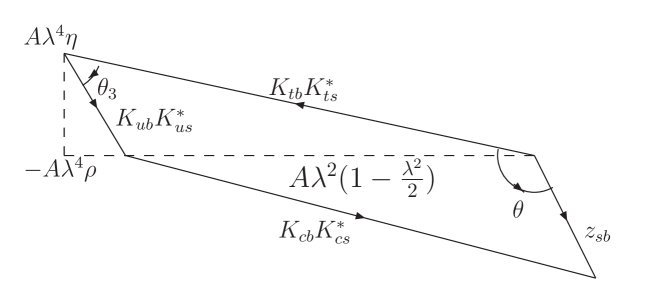
FIG. 1.: The quadrangle in $b\bar{s}$ sector.

III $b\to s\gamma$ and $b\to s\ell^{+}\ell^{-}$ transitions in VQM

In VQM, the down-type vector quark may be much heavier than weak scale. In a theory with different mass scales, the heavier scale should be integrated out firstly, then Wilson coefficients are run from heavier scale to low scale by using renormalization group equation. Only in case of $m_{D}$ is about the weak scale, can $W,Z$ boson, Higgs boson and top quark be integrated out together. In this work, we consider two possibilities as follows:

A Scenario A: $\delta_{D}=\frac{m^{2}_{Z,W,t,H}}{m_{D}^{2}}\ll 1$

In this scenario, we first integrate out the heavy $D$ quark, introducing dimension-5 and dimension-6 operators. By keeping only leading order terms of $\delta_{D}$, we obtain the effective Hamiltonian for $b\to s\gamma^{*}(g^{*})$ as:

$${\cal H}^{new}_{eff}(b\to\gamma^{*}(g^{*}))=\frac{4G_{F}}{\sqrt{2}}z_{4s}^{*}z_{4b}\sum_{i}C_{i}(\mu)O_{i}.$$ (33)

A complete basis for the local operators is listed below:

$$O_{LR}^{1} = -\frac{1}{16\pi^{2}}m_{b}\bar{s}_{L}{\cal D}^{2}b_{R},$$ (34)

$$O_{LR}^{2} = \frac{1}{16\pi^{2}}\mu^{\epsilon/2}g_{s}m_{b}\bar{s}_{L}\sigma^{\mu\nu}T^{a}b_{R}G_{\mu\nu},$$ (35)

$$O_{LR}^{3} = \frac{1}{16\pi^{2}}\mu^{\epsilon/2}ee_{d}m_{b}\bar{s}_{L}\sigma^{\mu\nu}b_{R}F_{\mu\nu},$$ (36)

$$Q_{LR}^{H} = \frac{1}{2}\mu^{\epsilon}g_{s}^{2}m_{b}H^{0}H^{0}\bar{s}_{L}b_{R},$$ (37)

$$Q_{LR}^{\chi} = \frac{1}{2}\mu^{\epsilon}g_{s}^{2}m_{b}\chi^{0}\chi^{0}\bar{s}_{L}b_{R},$$ (38)

$$P_{L}^{1,A} = -i\frac{1}{16\pi^{2}}\bar{s}_{L}T_{\mu\nu\sigma}^{A}{\cal D}^{\mu}{\cal D}^{\nu}{\cal D}^{\sigma}b_{R},$$ (39)

$$P_{L}^{2} = \frac{1}{16\pi^{2}}\mu^{\epsilon}\bar{s}_{L}\gamma^{\mu}b_{R}\partial^{\nu}F_{\mu\nu},$$ (40)

$$R_{L}^{1,H} = i\frac{1}{2}\mu^{\epsilon}g_{s}^{2}H^{0}H^{0}\bar{s}_{L}\not{\cal D}b_{L},$$ (41)

$$R_{L}^{1,\chi} = i\frac{1}{2}\mu^{\epsilon}g_{s}^{2}\chi^{0}\chi^{0}\bar{s}_{L}\not{\cal D}b_{L},$$ (42)

$$R_{L}^{2,H} = i\mu^{\epsilon}g_{s}^{2}({\partial}^{\sigma}H^{0})H^{0}\bar{s}_{L}\gamma_{\sigma}b_{L},$$ (43)

$$R_{L}^{2,\chi} = i\mu^{\epsilon}g_{s}^{2}({\partial}^{\sigma}\chi^{0})\chi^{0}\bar{s}_{L}\gamma_{\sigma}b_{L},$$ (44)

where $T^{a}$ stand for $SU(3)_{color}$ generators, $F_{\mu\nu}$ and $G_{\mu\nu}$ are field strength of photon and gluon respectively. The covariant derivative is given by

$${\cal D}_{\mu}=\partial_{\mu}-i\mu^{\epsilon/2}g_{s}G_{\mu}^{a}T^{a}-i\mu^{\epsilon/2}ee_{d}A_{\mu},$$ (45)

with $\epsilon=4-d$. The tensor $T_{\mu\nu\sigma}^{A}\ (A=1,2,3,4)$ appearing in $P_{L}^{1,A}$ have the following Lorentz structures [21, 22]:

$$T_{\mu\nu\sigma}^{1}=g_{\mu\nu}\gamma_{\sigma},\ \ \ T_{\mu\nu\sigma}^{2}=g_{\mu\sigma}\gamma_{\nu},\ \ \ T_{\mu\nu\sigma}^{3}=g_{\nu\sigma}\gamma_{\mu},\ \ \ T_{\mu\nu\sigma}^{4}=-i\epsilon_{\mu\nu\sigma\tau}\gamma^{\tau}\gamma_{5}.$$ (46)

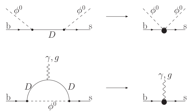
FIG. 2.: Matching conditions at scale $m_{D}$ in full theory (left) and in the intermediated effective field theory (right). $\phi^{0}$ can be $H^{0}$ and $\chi^{0}$.

To match the full theory into an effective theory, the diagrams to be matched at $m_{D}$ scale are displayed in Fig. 2. To determine the coefficients of the $\Gamma^{bs\phi\phi}$, $\Gamma^{bs\gamma\phi\phi}$, $\Gamma^{bsg\phi\phi}\ (\phi=H^{0},\chi^{0})$ at scale $m_{D}$, we just need to match the full theory with effective theory at tree level. We obtain

$$C_{Q_{LR}^{H}}(m_{D})=-C_{Q_{LR}^{\chi}}(m_{D})=-\frac{1}{g_{s}^{2}},$$ (47)

$$C_{R_{L}^{1,H}}(m_{D})=2C_{R_{L}^{2,H}}(m_{D})=-\frac{1}{2g_{s}^{2}},$$ (48)

$$C_{R_{L}^{1,\chi}}(m_{D})=2C_{R_{L}^{2,\chi}}(m_{D})=-\frac{1}{2g_{s}^{2}}.$$ (49)

Other coefficients can be determined by matching one loop diagrams shown in Fig. 2. After straightforward calculations, we have

$$C_{O_{LR}^{i}}(m_{D}) = 0\ \ (i=1,2,3),$$ (50)

$$C_{P_{L}^{1,1}}(m_{D}) = C_{P_{L}^{1,3}}(m_{D})=-\frac{11}{18},$$ (51)

$$C_{P_{L}^{1,2}}(m_{D}) = \frac{8}{9},$$ (52)

$$C_{P_{L}^{1,4}}(m_{D}) = -\frac{1}{2},$$ (53)

$$C_{P_{L}}^{2}(m_{D}) = 0.$$ (54)

The values are understood as sum of $H^{0},\ \chi^{0}$ contributions. Cancellation between Higgs and would-like Goldstone boson $\chi^{0}$ leads to $C_{O_{LR}}^{i}(m_{D})=0\ (i=1,2,3)$ in leading order.

The running of Wilson coefficients $C_{i}(\mu)$ from $m_{D}$ down to weak scale is governed by anomalous dimension $\gamma$ through RGE

$$\mu\frac{d}{d\mu}C_{i}(\mu)=\sum_{j}(\gamma^{T})_{ij}C_{j}(\mu).$$ (55)

We calculate one-loop diagrams with operator insertions and present the anomalous dimensions $\gamma$ in Appendix A. Using the anomalous dimensions (A4) and (A12), we can solve the RGE (55) and have the coefficients of the operators at weak scale $m_{W}^{+}$. They are given by,

$$C_{O_{LR}^{1}}(m_{W}^{+}) = \frac{247}{548}\zeta^{-\frac{4}{21}}+\frac{336}{8905}\zeta^{\frac{113}{126}}-\frac{551}{780}\zeta^{\frac{8}{21}}+\frac{1}{6}\zeta^{\frac{2}{3}},$$ (56)

$$C_{O_{LR}^{2}}(m_{W}^{+}) = \frac{247}{1096}\zeta^{-\frac{4}{21}}+\frac{168}{8905}\zeta^{\frac{113}{126}}-\frac{223}{780}\zeta^{\frac{8}{21}}+\frac{1}{24}\zeta^{\frac{2}{3}},$$ (57)

$$C_{O_{LR}^{3}}(m_{W}^{+}) = \frac{247}{1096}\zeta^{-\frac{4}{21}}+\frac{168}{8905}\zeta^{\frac{113}{126}}-\frac{223}{780}\zeta^{\frac{8}{21}}+\frac{5}{12}\zeta^{\frac{2}{3}}-\frac{3}{8}\zeta^{\frac{16}{21}},$$ (58)

$$C_{P_{L}^{1,1}}(m_{W}^{+}) = C_{P_{L}^{1,3}}(m_{W}^{+})=-\frac{247}{548}\zeta^{-\frac{4}{21}}-\frac{791}{4932}\zeta^{\frac{113}{126}},$$ (59)

$$C_{P_{L}^{1,2}}(m_{W}^{+}) = \frac{247}{548}\zeta^{-\frac{4}{21}}+\frac{1}{12}\zeta^{\frac{8}{21}}+\frac{875}{2466}\zeta^{\frac{113}{63}},$$ (60)

$$C_{P_{L}^{1,4}}(m_{W}^{+}) = -\frac{247}{598}\zeta^{-\frac{8}{21}}-\frac{1}{12}\zeta^{\frac{8}{21}}+\frac{14}{411}\zeta^{\frac{113}{126}},$$ (61)

$$C_{P_{L}^{2}}(m_{W}^{+}) = 0,$$ (62)

where $\zeta=\alpha_{s}(m_{D})/\alpha_{s}(m_{W}^{+})$.

In order to continue running the basis operator coefficients from $m_{W}$ scale down to $b$ quark scale, we use the effective QCD-corrected Hamiltonian obtained by integrating out the $W,Z$ bosons, would-be Goldstone boson, Higgs boson and top quark. The effective Hamiltonian describing $b\to sl^{+}l^{-}$ transition reads [5, 23]

$${\cal H}_{eff}(b\to sl^{+}l^{-}) = -\frac{4G_{F}}{\sqrt{2}}K_{tb}K^{*}_{ts}\left[\sum\limits_{i=1}^{10}{\widetilde{C}}_{i}(\mu){\cal Q}_{i}+\widetilde{C}_{7\gamma}(\mu){\cal Q}_{7\gamma}+\widetilde{C}_{8G}(\mu){\cal Q}_{8G}+{\cal C}_{9}(\mu){\cal O}_{9}+{\cal C}_{10}(\mu){\cal O}_{10}\right],$$ (63)

where

$${\cal Q}_{1} = (\bar{s}_{i}\gamma^{\mu}Lc_{j})(\bar{c}_{j}\gamma_{\mu}Lb_{i}),$$ (64)

$${\cal Q}_{2} = (\bar{s}\gamma^{\mu}Lc)(\bar{c}\gamma_{\mu}Lb),$$ (65)

$${\cal Q}_{3} = (\bar{s}\gamma^{\mu}Lb)\sum_{q}(\bar{q}\gamma_{\mu}Lq),$$ (66)

$${\cal Q}_{4} = (\bar{s}_{i}\gamma^{\mu}Lb_{j})\sum_{q}(\bar{q}_{j}\gamma_{\mu}Lq_{i}),$$ (67)

$${\cal Q}_{5} = (\bar{s}\gamma^{\mu}Lb)\sum_{q}(\bar{q}\gamma_{\mu}Rq),$$ (68)

$${\cal Q}_{6} = (\bar{s}_{i}\gamma^{\mu}Lb_{j})\sum_{q}(\bar{q}_{j}\gamma_{\mu}Rq_{i}),$$ (69)

$${\cal Q}_{7} = \frac{3}{2}(\bar{s}\gamma^{\mu}Lb)\sum_{q}e_{q}(\bar{q}\gamma_{\mu}Rq),$$ (70)

$${\cal Q}_{8} = \frac{3}{2}(\bar{s}_{i}\gamma^{\mu}Lb_{j})\sum_{q}e_{q}(\bar{q}_{j}\gamma_{\mu}Rq_{i}),$$ (71)

$${\cal Q}_{9} = \frac{3}{2}(\bar{s}\gamma^{\mu}Lb)\sum_{q}e_{q}(\bar{q}\gamma_{\mu}Lq),$$ (72)

$${\cal Q}_{10} = \frac{3}{2}(\bar{s}_{i}\gamma^{\mu}Lb_{j})\sum_{q}e_{q}(\bar{q}_{j}\gamma_{\mu}Lq_{i}),$$ (73)

$${\cal Q}_{7\gamma} = \frac{e}{16\pi^{2}}m_{b}\bar{s}_{i}\sigma^{\mu\nu}Rb_{i}F_{\mu\nu},$$ (74)

$${\cal Q}_{8G} = \frac{g_{s}}{16\pi^{2}}\bar{s}_{i}\sigma^{\mu\nu}RT_{ij}^{a}b_{j}G^{a}_{\mu\nu},$$ (75)

$${\cal O}_{9} = \frac{e^{2}}{16\pi^{2}}(\bar{s}\gamma^{\mu}Lb)(\bar{l}\gamma_{\mu}l),$$ (76)

$${\cal O}_{10} = \frac{e^{2}}{16\pi^{2}}(\bar{s}\gamma^{\mu}Lb)(\bar{l}\gamma_{\mu}\gamma_{5}l).$$ (77)

To match the operator set in (44) onto these operators, we use the equations of motion to reduce all remaining two-quark operators to the gluon and photon magnetic moment operators $O_{LR}^{2}$ and $O_{LR}^{3}$ which are redefined as ${\cal Q}_{8G}$ and ${\cal Q}_{7\gamma}$ in (77).

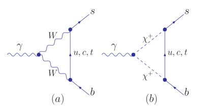
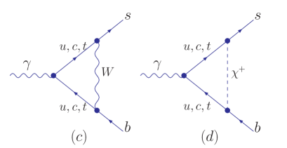
FIG. 3.: Charged boson mediated penguin diagram contributing to $b\to s\gamma$.

Firstly, we present the values of the Wilson coefficients at $m_{W}$ scale calculated in NDR and HV schemes as follows with small $V_{ub}V_{us}^{*}$ omitted:

$${\widetilde{C}}_{1}(m_{W}) = \frac{11}{2}(1+2\xi)\frac{\alpha_{s}(m_{W})}{4\pi},$$ (78)

$${\widetilde{C}}_{2}(m_{W}) = 1-\frac{z_{sb}}{K_{tb}K_{ts}^{*}}-\frac{11}{6}(1+2\xi)\frac{\alpha_{s}(m_{W})}{4\pi}-\frac{35}{18}\frac{\alpha_{em}}{4\pi},$$ (79)

$${\widetilde{C}}_{3}(m_{W}) = -\frac{1}{6}\frac{z_{sb}}{K_{tb}K_{ts}^{*}}-\frac{1}{6}\frac{\alpha_{s}(m_{W})}{4\pi}\left[E(x_{t})+\frac{2}{3}\xi\right]+\frac{\alpha_{em}}{6\pi}\frac{2B(x_{t})+C(x_{t})}{\sin^{2}\theta_{W}},$$ (80)

$${\widetilde{C}}_{4}(m_{W}) = -3{\widetilde{C}}_{5}(m_{W})={\widetilde{C}}_{6}(m_{W})=-\frac{1}{2}\left[E(x_{t})+\frac{2}{3}\xi\right]\frac{\alpha_{s}(m_{W})}{4\pi},$$ (81)

$${\widetilde{C}}_{7}(m_{W}) = -\frac{2}{3}\sin^{2}\theta_{W}\frac{z_{sb}}{K_{tb}K_{ts}^{*}}+\frac{\alpha_{em}}{6\pi}\left[4C(x_{t})+D(x_{t})-\frac{4}{9}(1+\xi)\right],$$ (82)

$${\widetilde{C}}_{8}(m_{W}) = {\widetilde{C}}_{10}(m_{W})=0,$$ (83)

$${\widetilde{C}}_{9}(m_{W}) = -\frac{2}{3}\cos^{2}\theta_{W}\frac{z_{sb}}{K_{tb}K_{ts}^{*}}+\frac{\alpha_{em}}{6\pi}\left[\frac{10B(x_{t})-4C(x_{t})}{\sin^{2}\theta_{W}}+4C(x_{t})+D(x_{t})-\frac{4}{9}(1+\xi)\right],$$ (84)

$${\widetilde{C}}_{7\gamma}(m_{W}) = -\frac{1}{2}A(x_{t})+\frac{z_{sb}}{K_{tb}K_{ts^{*}}}\left[\frac{23}{36}-\frac{1}{2}C_{O_{LR}^{1}}(m_{W}^{+})+C_{O_{LR}^{3}}(m_{W}^{+})-\frac{1}{4}C_{P_{L}^{1,2}}(m_{W}^{+})+\frac{1}{4}C_{P_{L}^{1,4}}\right.$$ (86)

$$\left.+e_{d}\left(\frac{1}{3}+\frac{1}{9}\sin^{2}\theta_{W}\right)\right]$$

$${\widetilde{C}}_{8G}(m_{W}) = -\frac{1}{2}F(x_{t})+\frac{z_{sb}}{K_{tb}K_{ts^{*}}}\left[\frac{1}{3}-\frac{1}{2}C_{O_{LR}^{1}}(m_{W}^{+})+C_{O_{LR}^{2}}(m_{W}^{+})-\frac{1}{2}C_{P_{L}^{1,1}}(m_{W}^{+})-\frac{1}{4}C_{P_{L}^{1,2}}(m_{W}^{+})\right.$$ (88)

$$\left.+\frac{1}{4}C_{P_{L}^{1,4}}-3e_{d}\left(\frac{1}{3}+\frac{1}{9}\sin^{2}\theta_{W}\right)\right],$$

$${\cal C}_{9}(m_{W}) = \frac{\pi}{\alpha_{em}}\frac{z_{sb}}{K_{tb}K_{ts}^{*}}(-1+4\sin^{2}\theta_{W})+\frac{C(x_{t})-B(x_{t})}{\sin^{2}\theta_{W}}-4C(x_{t})-D(x_{t})+\frac{4}{9}(1+\xi)+O\left(\frac{z_{sb}}{K_{tb}K_{ts}^{*}}\right),$$ (89)

$${\cal C}_{10}(m_{W}) = \frac{\pi}{\alpha_{em}}\frac{z_{sb}}{K_{tb}K_{ts}^{*}}+\frac{B(x_{t})-C(x_{t})}{\sin^{2}\theta_{W}}+O\left(\frac{z_{sb}}{K_{tb}K_{ts}^{*}}\right),$$ (90)

where $\xi=0$ in NDR scheme and $\xi=-1$ in HV scheme. The loop functions can be found in Appendix B.

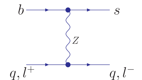
FIG. 4.: Tree level Feynman diagram contributing to $b\to s\gamma$ and $b\to sl^{+}l^{-}$.

The terms proportional to $\frac{z_{sb}}{K_{tb}K_{ts}^{*}}$ in ${\widetilde{C}}_{3,7,9}(m_{W})$ and the first term of ${\cal C}_{9,10}(m_{W})$ come from the tree-level diagram as displayed in Fig. 4, the term proportional to $\frac{z_{sb}}{K_{tb}K_{ts}^{*}}$ in ${\widetilde{C}}_{2}(m_{W})$ comes from tree diagram due to the non-unitarity of CKM matrix in VQM. In expressions of ${\widetilde{C}}_{7\gamma,8G}(m_{W})$, the first constant terms proportional to $\frac{z_{sb}}{K_{tb}K_{ts}^{*}}$ come from the charged current one-loop diagram Fig. 3 due to the non-unitarity of CKM matrix in VQM, other terms proportional to $\frac{z_{sb}}{K_{tb}K_{ts}^{*}}$ come from the neutral current one-loop diagrams shown in Fig. 5. As in expressions ${\cal C}_{9,10}(m_{W})$, the second terms proportional to $\frac{z_{sb}}{K_{tb}K_{ts}^{*}}$ denoted as $O\left(\frac{z_{sb}}{K_{tb}K_{ts}^{*}}\right)$ come from the charged and neutral current one-loop diagrams. In deriving above equation, we have used the unitarity relation

$$z_{4b}z_{4s}^{*}=-z_{sb}$$ (91)

which is a direct result of Eq. (4).

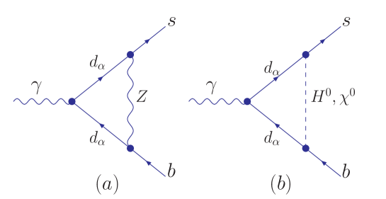
FIG. 5.: Neutral boson mediated penguin diagram contributing to $b\to s\gamma$.

At this moment, we would like to point out that the contributions from the $Z$-penguin charged current one-loop diagrams in the VQM to ${\cal C}_{9,10}(m_{W})$, have divergent terms due to the non-unitarity of CKM matrix. Although these divergences can be removed by renormalizing the tree level FCNC which exists in VQM Lagrangian, they are scheme dependent. However, these scheme dependences are subleading compared to the first terms of ${\cal C}_{9,10}(m_{W})$, which we will neglect them in our calculation. Under this approximation they are not relevant for the inclusive dileptonic decays.

B Scenario B: $\delta_{D}=\frac{m^{2}_{Z,W,t,H}}{m_{D}^{2}}\sim 1$

In this scenario, the top and $D$ quark, W and Z bosons can be integrated out together. The corresponding initial values of Wilson coefficients ${\widetilde{C}}_{7\gamma,8G}(m_{W})$ are changed to [10]

$${\widetilde{C}}_{7\gamma}(m_{W}) = -\frac{1}{2}A(x_{t})+\frac{z_{sb}}{K_{tb}K_{ts}^{*}}\left[\frac{23}{36}+\left(f_{D}^{Z}(y_{D})+f_{D}^{H}(w_{D})+f_{D}^{\chi}(y_{D})\right)+e_{d}\left(\frac{1}{3}+\frac{1}{9}\sin^{2}\theta_{W}\right)\right],$$ (92)

$${\widetilde{C}}_{8G}(m_{W}) = -\frac{1}{2}F(x_{t})+\frac{z_{sb}}{K_{tb}K_{ts}^{*}}\left[\frac{1}{3}-3\left(f_{D}^{Z}(y_{D})+f_{D}^{H}(w_{D})+f_{D}^{\chi}(y_{D})\right)-3e_{d}\left(\frac{1}{3}+\frac{1}{9}\sin^{2}\theta_{W}\right)\right].$$ (93)

where $y_{D}=m_{D}^{2}/m_{Z}^{2},\ w_{D}=m_{D}^{2}/m_{H}^{2}$. Other Wilson coefficients are the same as Scenario A we discussed. The functions $f_{y}^{x}$ stands for the contribution from boson $x$ mediated penguin one-loop diagram with quark $y$ in loops and are presented in Appendix B.

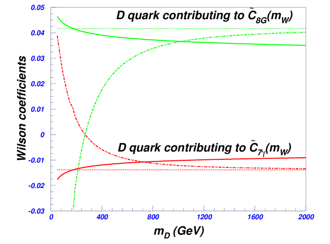
FIG. 6.: The down-type vector quark contributions to Wilson coefficients of ${\cal Q}_{7\gamma}$ and ${\cal Q}_{8G}$ at $m_{W}$ scale in unit of $\frac{z_{sb}}{K_{tb}K_{ts}^{*}}$ $(m_{H}=m_{t})$. The solid and dashed lines stand for the results in Scenario A with or without consideration of QCD running effect from $m_{D}$ to $m_{W}$, respectively. The corresponding values in Scenario B are denoted by dot-dashed lines.

In Fig.6 we plot the down-type vector quark contribution to the Wilson coefficients ${\widetilde{C}}_{7\gamma}$ and ${\widetilde{C}}_{8G}$ as a function $m_{D}$ at $m_{W}$ scale, and demonstrate the QCD running effects from $m_{D}$ down to $m_{W}$ in Scenario A.

As a consistency check, we can see that if the QCD correction is neglected by setting $\zeta=1$ and only leading order terms of $\delta_{D}$ are kept, for on-shell quarks and photon, our results ${\widetilde{C}}_{7\gamma}(m_{W})$ and ${\widetilde{C}}_{8G}(m_{W})$ in Scenario A would produce the results exactly in Scenario B.

At the end of this subsection, we make some emphasis on the results obtained by using different approaches as follows:

The effect of running from $m_{D}$ down to weak scale on the contributions from neutral current mediated by $D$ quark in Scenario A is large, as shown in Fig. 6. However, at $m_{W}$ scale, since dominant new contribution comes from the charged current diagrams, the total results of ${\widetilde{C}}_{7\gamma,8G}(m_{W})$ are changed slightly. This indicates that the dependence of the branching ratio of $B\to X_{s}\gamma$ on $m_{D}$ is quite weak in both Scenarios. Therefore, we can not extract the mass of down-type vector quark from this analysis.

IV Constraints on $z_{sb}$ in VQM from inclusive decays $B\to X_{s}\ell^{+}\ell^{-}$

A Solutions of Wilson coefficients

To obtain some predictions for inclusive $B$ rare decays, we need to determine the Wilson coefficients at $m_{b}$ scale. Expanding anomalous dimension matrix and Wilson coefficient as

$$\gamma = \gamma^{(0)}\frac{\alpha_{s}(\mu)}{4\pi}+\gamma^{(1)}(\frac{\alpha_{s}(\mu)}{4\pi})^{2}+\cdots,$$ (94)

$$C(\mu) = C^{(0)}(\mu)+C^{(1)}(\mu)\frac{\alpha_{s}(m_{W})}{4\pi}+\cdots,$$ (95)

we solve the Wilson coefficients up to order $\alpha_{s}(m_{W})$ according to the RGE (55). The relevant $10\times 10$ one-loop anomalous dimension matrix among ${\cal Q}_{1-10}$, $\gamma^{(0)}$, and two-loop anomalous dimension matrices among ${\cal Q}_{1-10}$ with ${\cal Q}_{7\gamma,8G}$ and ${\cal O}_{9}$ needed in our calculations are collected in Appendix A.

Using the $10\times 10$ matrix $\gamma^{(0)}$ in Appendix, and initial values presented in Section II, we obtain the solutions

$${\widetilde{C}}_{i}^{(0)}(\eta) = \sum\limits_{i,l=1}^{10}{\hat{V}}^{-1}_{il}\eta^{a_{l}}{\hat{V}}_{l2}-\frac{z_{sb}}{K_{tb}K_{ts}^{*}}{\hat{V}}^{-1}_{il}\sum\limits_{l}^{10}\eta^{a_{l}}\left[{\hat{V}}_{l2}+\frac{1}{6}{\hat{V}}_{l3}+\frac{2}{3}\sin^{2}\theta_{W}{\hat{V}}_{l7}+\frac{2}{3}\sin^{2}\theta_{W}{\hat{V}}_{l9}\right].$$ (96)

where $\eta=\alpha_{s}(m_{W})/\alpha_{s}(\mu),\ {\widetilde{C}}_{k}^{(0)}(1)\equiv{\widetilde{C}}_{k}^{(0)}(m_{W})$. The eigenvalues $a_{l}$ are obtained by diagonalizing the $10\times 10$ anomalous dimension matrix $\frac{\gamma^{(0)}}{2\beta_{0}}$,

$$({\hat{V}}\frac{\gamma^{(0)}}{2\beta_{0}}{\hat{V}}^{-1})_{lj}=a_{l}\delta_{lj}.$$ (97)

At leading order, the solution of ${\widetilde{C}}_{7\gamma}(\eta)$ is given by

$${\widetilde{C}}_{7\gamma}(\eta) = \eta^{\frac{\gamma_{\gamma\gamma}}{2\beta_{0}}}{\widetilde{C}}_{7\gamma}(m_{W})+\frac{\gamma_{G\gamma}}{\gamma_{GG}-\gamma_{\gamma\gamma}}\left(\eta^{\frac{\gamma_{GG}}{2\beta_{0}}}-\eta^{\frac{\gamma_{\gamma\gamma}}{2\beta_{0}}}\right){\widetilde{C}}_{8G}(m_{W})$$ (100)

$$-\frac{\gamma_{G\gamma}}{\gamma_{GG}-\gamma_{\gamma\gamma}}\left(\eta^{\frac{\gamma_{GG}}{2\beta_{0}}}-\eta^{\frac{\gamma_{\gamma\gamma}}{2\beta_{0}}}\right)\frac{\beta_{\gamma i}}{2\beta_{0}}\hat{V}_{il}^{-1}\frac{1}{a_{l}-\frac{\gamma_{GG}}{2\beta_{0}}}{\hat{V}}_{lk}{\widetilde{C}}_{k}^{(0)}(1)$$

$$+\hat{V}_{il}^{-1}\left[\frac{\beta_{\gamma i}}{2\beta_{0}}+\frac{\gamma_{G\gamma}}{2\beta_{0}}\frac{\beta_{Gi}}{2\beta_{0}}\frac{1}{a_{l}-\frac{\gamma_{GG}}{2\beta_{0}}}\right]\frac{\eta^{a_{l}}-\eta^{\frac{\gamma_{\gamma\gamma}}{2\beta_{0}}}}{a_{l}-\frac{\gamma_{\gamma\gamma}}{2\beta_{0}}}{\hat{V}}_{lk}{\widetilde{C}}_{k}^{(0)}(1).$$

For ${\cal C}_{9}^{(0)}(\eta)$, the corresponding solution is

$${\cal C}_{9}^{(0)}(\eta) = \frac{z_{sb}}{K_{tb}K_{ts}^{*}}\left[\frac{\pi}{\alpha_{em}}(-1+4\sin^{2}\theta_{W})+\frac{\pi}{\alpha_{s}(m_{W})}\sum_{l=1}^{10}\bar{p}_{l}(\eta^{a_{l}}-1)\right]+\frac{\pi}{\alpha_{s}(m_{W})}\sum_{l=1}^{10}p_{l}(\eta^{a_{l}}-1).$$ (101)

where

$$p_{l} = \sum_{i=1}^{10}\frac{\gamma^{(0)}_{i,11}}{\beta_{0}}\hat{V}^{-1}_{il}\hat{V}_{l2},$$ (102)

$$\bar{p}_{l} = -\sum_{i=1}^{10}\frac{\gamma^{(0)}_{i,11}}{\beta_{0}}\hat{V}^{-1}_{il}\left[{\hat{V}}_{l2}+\frac{1}{6}{\hat{V}}_{l3}+\frac{2}{3}\sin^{2}\theta_{W}{\hat{V}}_{l7}+\frac{2}{3}\sin^{2}\theta_{W}{\hat{V}}_{l9}\right].$$ (103)

To obtain the scheme independent one-loop matrix element of ${\cal O}_{9}$ in VQM, calculation up to next-to-leading order (NLO) is necessary, as the case of SM. To obtain ${\cal C}_{9}(\mu)$ , we frist present the NLO calculations for ${\tilde{C}}_{i}(\mu)$ as

$${\widetilde{C}}_{i}^{(1)}(\eta) = {\hat{V}}^{-1}_{il}\eta^{a_{l}}{\hat{V}}_{lk}{\widetilde{C}}_{k}^{(1)}(1)+{\hat{V}}^{-1}_{il}\left[{\hat{V}}\frac{\gamma^{(1)T}}{2\beta_{0}}{\hat{V}}^{-1}\right]_{lj}\frac{\eta^{a_{j}-1}-\eta^{a_{l}}}{a_{j}-a_{l}-1}{\hat{V}}_{jk}{\widetilde{C}}_{k}^{(0)}(1)$$ (105)

$$+\frac{\beta_{1}}{\beta_{0}}{\hat{V}}^{-1}_{il}a_{l}\left(\eta^{a_{l}-1}-\eta^{a_{l}}\right){\hat{V}}_{lk}{\widetilde{C}}_{k}^{(0)}(1).$$

The solution of $C_{9}(\eta)$ in NDR scheme is

$${\cal C}_{9}(\eta) =\frac{z_{sb}}{K_{tb}K_{ts}^{*}}\left[\frac{\pi}{\alpha_{em}}(-1+4\sin^{2}\theta_{W})+\frac{\pi}{\alpha_{s}(m_{W})}\sum_{l=1}^{10}\bar{p}_{l}(\eta^{a_{l}}-1)\right]+\frac{\pi}{\alpha_{s}(m_{W})}\sum_{l=1}^{10}p_{l}(\eta^{a_{l}}-1)$$ (108)

$$+\left[\frac{C(x_{t})-B(x_{t})}{\sin^{2}\theta_{W}}-4C(x_{t})-D(x_{t})+\frac{4}{9}(1+\xi)\right]$$

$$+\sum_{l}\left[\left(\eta^{a_{l}}-1\right)r_{l}+(s_{l}+q_{l}E(x_{t}))\left(\eta^{a_{l}+1}-1\right)\right].$$

The numerical results for parameters $a_{l},p_{l},\bar{p}_{l},s_{l},q_{l}$ are follows:

$$a_{l} = (-0.8994,-0.5217,-0.4230,0.1457,0.2609,0.4087,0.1304,-1.4034),$$ (109)

$$p_{l} = (0.1648,0.2424,0.1384,-0.0073,-0.3941,0.0433,0,0),$$ (110)

$$\bar{p}_{l} = (-0.0248,1.0004,0.0853,0.0207,1.6602,-0.0690,0.5223,-1.6974),$$ (111)

$$s_{l} = (-0.3554,-0.3579,-0.3617,0.0072,-0.2009,0.0490,0,0),$$ (112)

$$q_{l} = (-0.2701,0,0.0918,,0.0059,0,0.0318,0,0),$$ (113)

$$r_{l}^{NDR} = (-0.0292,-0.1960,0.1328,-0.1858,0.8997,-0.2011,0,0).$$ (114)

One can check that in case of $z_{sb}=0$, the results are the same as those in SM [26].

Note four-quark operators ${\cal Q}_{1-10}$ can contribute to one-loop matrix element of ${\cal O}_{9}$. Defining the effective coefficient ${\cal C}_{9}^{eff}$ as

$${\cal C}_{9}^{eff}<sl^{+}l^{-}|{\cal O}_{9}|b>\equiv{\cal C}_{9}(\eta)<sl^{+}l^{-}|{\cal O}_{9}|b>+\sum_{i=1}^{10}C_{i}^{(0)}(\eta)<sl^{+}l^{-}|{\cal Q}_{i}|b>,$$ (115)

we obtain $C_{9}^{eff}(\eta)$ in VQM as

$$C_{9}^{eff} = \frac{z_{sb}}{K_{tb}K_{ts}^{*}}\left[\frac{\pi}{\alpha_{em}}(-1+4\sin^{2}\theta_{W})+\frac{\pi}{\alpha(m_{W})}\sum_{l}\bar{p}_{l}(\eta^{a_{l}+1}-1)\right]$$ (119)

$$+\frac{\pi}{\alpha_{s}(m_{W})}\sum_{l}p_{l}(\eta^{a_{l}+1}-1)+\left[\frac{C(x_{t})-B(x_{t})}{\sin^{2}\theta_{W}}-4C(x_{t})-D(x_{t})+\frac{4}{9}\right]$$

$$+\sum_{l}\left[\left(\eta^{a_{l}}-1\right)r^{NDR}_{l}+(s_{l}+q_{l}E(x_{t}))\left(\eta^{a_{l}+1}-1\right)\right]$$

$$+h(\frac{m_{c}^{2}}{m_{b}^{2}},s)T_{9}^{c(0)}+h(1,s)T_{9}^{b(0)}-\frac{1}{2}h(0,s)\left[{\tilde{C}}^{(0)}_{3}+3{\tilde{C}}^{(0)}_{4}\right]+\frac{9}{2}\left[3{\tilde{C}}^{(0)}_{3}+{\tilde{C}}^{(0)}_{4}+3{\tilde{C}}^{(0)}_{5}+{\tilde{C}}^{(0)}_{6}\right],$$

where $s$ is dilepton mass squared normalized by $m_{b}^{2}$, and

$$T_{9}^{c(0)} = 3{\tilde{C}}_{1}^{(0)}+{\tilde{C}}^{(0)}_{2}+3{\tilde{C}}^{(0)}_{3}+{\tilde{C}}^{(0)}_{4}+3{\tilde{C}}^{(0)}_{5}+{\tilde{C}}^{(0)}_{6},$$ (120)

$$T_{9}^{b(0)} = -\frac{1}{2}\left[4{\tilde{C}}^{(0)}_{3}+4{\tilde{C}}^{(0)}_{4}+3{\tilde{C}}^{(0)}_{5}+{\tilde{C}}^{(0)}_{6}\right].$$ (121)

The function $h(z,s)$ which includes light quark-antiquark pair contributions has an expression as

$$h(z,s) = -\frac{8}{9}\ln\frac{m_{b}}{\mu}-\frac{8}{9}\ln z+\frac{8}{27}-\frac{4}{9}x-\frac{2}{9}(2+x)|1-x|^{\frac{1}{2}}$$ (125)

$$\times\left\{\begin{array}[]{ll}\ln\left|\frac{\sqrt{1-x}+1}{\sqrt{1-x}-1}\right|-i\pi&for\ x\equiv 4\frac{z^{2}}{s}<1,\\ 2\arctan\frac{1}{\sqrt{x-1}}&for\ x\equiv 4\frac{z^{2}}{s}>1.\\ \end{array}\right.$$

Now we consider the long distance contributions to ${\cal C}_{9}^{eff}$. Apart from $J/\Psi$ family, resonance $\phi$ should be added to long distance part of ${\cal C}^{eff}_{9}$ due to tree level $Z\bar{s}b$ coupling. Similar to previous analysis [27], the non-perturbative contributions can be parameterized as

$$Y_{Res}(s) = \frac{3\pi}{\alpha_{em}^{2}}\left[T^{s(0)}\frac{\Gamma[\phi\to\ell^{+}\ell^{-}]m_{\phi}}{m^{2}_{\phi}-sm_{B}^{2}-m_{\phi}\Gamma_{\phi}}+T^{c(0)}_{9}\kappa\sum\limits_{i=1}^{6}\frac{\Gamma[\Psi(is)\to\ell^{+}\ell^{-}]m_{\Psi(is)}}{m^{2}_{\Psi(is)}-sm_{B}^{2}-im_{\Psi(is)}\Gamma_{\Psi(is)}}\right],$$ (126)

$${\cal C}_{9}^{eff} \to{\cal C}_{9}^{eff}+Y_{Res}(s).$$ (127)

Here $\kappa=2.3$ is a phenomenological factor, $|T^{c(0)}_{9}\kappa|$ can be fixed from the $J/\Psi,\Psi^{\prime}$ data. $T^{s(0)}_{9}$ and $T^{c(0)}_{9}$ correspond to the coefficients of $h(\frac{m_{s}^{2}}{m_{b}^{2}},s)$ and $h(\frac{m_{c}^{2}}{m_{b}^{2}},s)$ in expression of ${\cal C}_{9}^{eff}$ respectively, $T^{s(0)}_{9}=T^{b(0)}$. Since experimental measurement for $B\to X_{s}\phi$ is not available so far, we set the phenomenological factor for $\phi$ to be unity in our numerical calculation.

B Constraints on $z_{sb}$ from inclusive decays $B\to X_{s}\ell^{+}\ell^{-}$

With all Wilson coefficients at $b$ quark mass scale ready, the invariant dilepton distribution for $B\to X_{s}\ell^{+}\ell^{-}$ can be expressed in terms of the effective Wilson coefficients defined above as

$$\frac{d\Gamma(B\to X_{s}l^{+}l^{-})}{ds} = \left(\frac{\alpha_{em}}{4\pi}\right)^{2}\frac{G_{F}^{2}m_{b}^{5}|K_{ts}^{*}K_{tb}|^{2}}{48\pi^{3}}(1-s)^{2}R_{0}$$ (128)

where

$$R_{0} = 4\left(1+\frac{2}{s}\right)|{\widetilde{C}}^{eff}_{7\gamma}|^{2}+(1+2s)\left(|{\cal C}_{9}^{eff}|^{2}+|{\cal C}_{10}|^{2}\right)+12Re({\widetilde{C}}^{eff}_{7\gamma}{\cal C}_{9}^{eff*}),$$ (129)

where ${\widetilde{C}}^{eff}_{7\gamma}$ is determined by Eq. (100) using the vectors $\beta_{\gamma}$ and $\beta_{G}$ calculated in HV scheme.

Now we constrain the parameter $z_{sb}$ from $B\to X_{s}l^{+}l^{-}$. The branching ratio of $B\to X_{s}l^{+}l^{-}$ depends on the tree level FCNC coupling $z_{sb}$ and $|K_{tb}K_{ts}|$. $|K_{tb}K_{ts}|$ can be written in terms of $|K_{cb}K_{cs}|$ and $z_{sb}$. In fact, from the quadrangle in $b\bar{s}$ sector, Fig. 1, one can derive the relation,

$$|K_{tb}K_{ts}^{*}|=|K_{cb}K_{cs}^{*}|+|K_{ub}K_{us}^{*}|\cos\theta_{3}+|z_{sb}|\cos\theta,$$ (130)

$$\theta=arg\left(\frac{z_{sb}}{K_{tb}K_{ts}^{*}}\right),\ \ \ \theta_{3}=arg\left(-\frac{K_{ub}K_{us}^{*}}{K_{tb}K_{ts}^{*}}\right).$$ (131)

We use Eq. (131) to determine $|K_{tb}K_{ts}|$ in Eq. (128). Then, from the branching ratios of $B\to X_{s}l^{+}l^{-}$, one can derive the constraints on $|z_{sb}|$ and $\theta$. In the relation Eq. (131), for $|K_{cb}K_{cs}|$, we have used the experimental values shown in Table I. $|K_{ub}K_{us}|$ in Eq. (131) was neglected in the numerical calculation. Integrating Eq.(128), we exclude the resonances $J/\Psi,\Psi^{\prime}$ contributions by using the same cuts as experiments[8] $0.20<|m_{l^{+}l^{-}}-m_{J/\Psi}|<0.35,\quad 0.15<|m_{l^{+}l^{-}}-m_{\Psi^{\prime}}|<0.30.$ The corresponding $2\sigma$ experimental bounds on the size of $z_{sb}$ and phase $\theta$ from experimental measurement for $B\to X_{s}l^{+}l^{-}$ are displayed in Fig.7. From this figure, we obtain

$$|z_{sb}|\leq 1.40\times 10^{-3}\ (95\%\ \ C.L.).$$ (132)

One can see clearly that the absolute value of the allowed phase $\theta$ becomes smaller as the size of $z_{sb}$ increases.

TABLE I.: Input parameters are used in calculation. All masses in unit of GeV.

$\alpha_{s}(m_{Z})$	0.119	$\alpha_{em}$	1/133
$m_{Z}$	91.19	$\lambda_{2}$	$0.12\ GeV^{2}$
$m_{W}$	80.41	$Br^{ex}(B\to X_{c}e\nu)$	0.104
$m_{b}^{pole}$	4.8	$|K_{us}|$	$0.2196\pm 0.0026$
$m_{t}^{pole}$	$173.8\pm 5$	$|K_{cs}|$	$0.97\pm 0.11$
$m_{c}/m_{b}$	$0.29\pm 0.2$	$|K_{ub}|$	$(3.6\pm 0.7)\times 10^{-3}$
$m_{s}/m_{b}$	0.02	$|K_{cb}|$	$(4.12\pm 0.2)\times 10^{-2}$
$\sin^{2}\theta_{W}$	0.231	$G_{F}$	$1.166\times 10^{-5}\ GeV^{-2}$

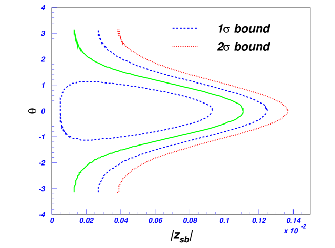
FIG. 7.: The ($|z_{sb}|,\theta$) contour in $Scenario\ A$ constrained by $Br^{ex}(B\to X_{s}l^{+}l^{-})$. The dashed, dotted lines correspond to $1\sigma$ and $2\sigma$ experimental bounds of $B\to X_{s}l^{+}l^{-}$ in (1), respectively. The solid line denotes the experimental central value $6.2\times 10^{-6}$. The region between dot lines is allowed at $1\sigma$ level.

V Some predictions for $B\to X_{s}\ell^{+}\ell^{-}$ and $B\to X_{s}\gamma$

In this section, subject to the constraints on $z_{sb}$ from $B\to X_{s}l^{+}l^{-}$, we will present predictions for the invariant dilepton mass distribution, FB asymmetry, the zero point of FB asymmetry of $B\to X_{s}l^{+}l^{-}$, and the branching ratio of $B\to X_{s}\gamma$.

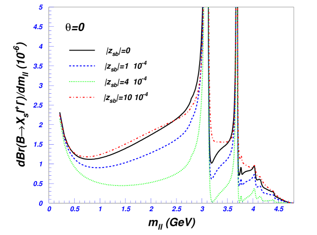
FIG. 8.: The differential rate of $B\to X_{s}l^{+}l^{-}$ normalized by $Br(B\to X_{c}l\nu)$ as a function of dilepton invariant mass.

Firstly, we consider the invariant dilepton mass distribution of $B\to X_{s}l^{+}l^{-}$. According to the study in subsection IV A, it is expected to be sensitive to the parameter $z_{sb}$. This feature is shown in Fig.8.

In addition to the differential and total branching ratio, the forward-backward (FB) asymmetry can provide crucial information on new physics. The normalized FB asymmetry distribution is defined as

$$\bar{A}_{FB} = \frac{\int d{\hat{\theta}}\frac{d^{2}\Gamma(b\to sl^{+}l^{-})}{dsd\cos{\hat{\theta}}}sign(\cos{\hat{\theta}})}{\int d{\hat{\theta}}\frac{d^{2}\Gamma(b\to sl^{+}l^{-})}{dsd\cos{\hat{\theta}}}}=-\frac{3}{R_{0}}Re[(s{\cal C}^{eff}_{9}+2{\tilde{C}}_{7\gamma}){\cal C}_{10}^{*}].$$ (133)

Thus, the zero of the FB asymmetry $s_{0}$ in VQM is determined by equation

$$Re\left[\left(s_{0}{\cal C}^{eff}_{9}+2{\widetilde{C}}^{eff}_{7\gamma}\right){\cal C}_{10}^{*}\right]=0.$$ (134)

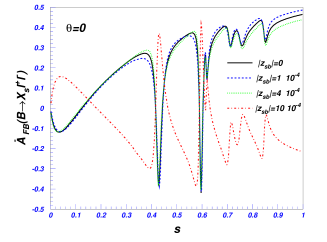
FIG. 9.: The FB asymmetry of $B\to X_{s}l^{+}l^{-}$ distribution.

It is very interesting to analyze how the zero of the FB asymmetry ($s_{0}$) is modified in VQM. Unlike to the case of SM where ${\cal C}_{10}$ is real, the coefficient ${\cal C}_{10}$ is complex generally in VQM. Furthermore, the contributions to ${\cal C}_{9,10}$ from tree level FCNC diagram

$$|{\cal C}_{10}^{Tree}(m_{W})|=\frac{\pi}{\alpha_{em}}\left|\frac{z_{sb}}{K_{tb}K_{ts}^{*}}\right|\gg|{\cal C}_{9}^{Tree}(m_{W})|=\frac{\pi}{\alpha_{em}}\left|\frac{z_{sb}}{K_{tb}K_{ts}^{*}}\right|(1-4\sin^{2}\theta_{W}),$$ (135)

indicate that ${\cal C}_{10}$ can have large imaginary part. Therefore, $s_{0}$ in VQM will have large deviation from that in SM.

As an illustration, we plot the FB asymmetry as a function of $s$ in Fig. 9 corresponding to different size of $z_{sb}$. To show how the zero point $s_{0}$ sensitive to both the size of $z_{sb}$ and phase $\theta$, we display the dependence of zero point of FB asymmetry on $z_{sb}$ in Fig. 10. Figs.9 and 10 indicate that, subject to the experimental measurement for branching ratio of $B\to X_{s}l^{+}l^{-}$, FB asymmetry distribution and the zero point of FB asymmetry are very sensitive to the parameters $z_{sb}$ and phase $\theta$, especially in the region $0.6\times 10^{-3}<|z_{sb}|<1.2\times 10^{-3}.$

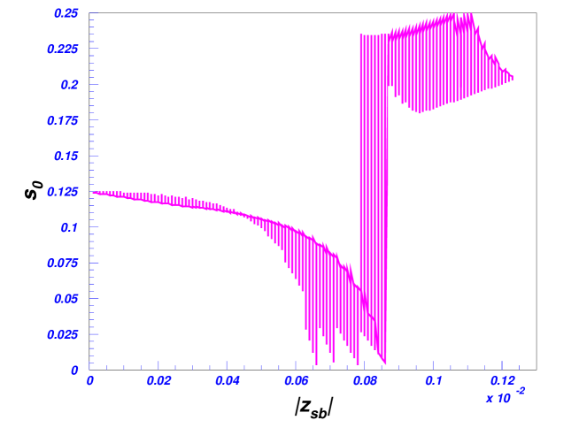
FIG. 10.: The $(|z_{sb}|,s_{0})$ contour in VQM subject to the $1\sigma$ bounds of $Br^{ex}(B\to X_{s}l^{+}l^{-})$. For specified $|z_{sb}|$, the phase $\theta$ effect on $s_{0}$ is also shown.

Now we study the radiative decay $B\to X_{s}\gamma$. The Branching ratio of $B\to X_{s}\gamma$ can be expressed as

$${\cal B}r(B\to X_{s}\gamma) = {\cal B}r^{ex}(B\to X_{c}e\bar{\nu}_{e})R_{quark}({\delta}^{max})\left[1-6\left(1-\frac{(1-z)^{4}}{g(z)}\right)\lambda_{2}\right],$$ (136)

where $z=m_{c}^{2}/m_{b}^{2},\ g(z)=1-8z+8z^{3}-z^{4}-12z^{2}\ln z$ is the phase space factor. ${\delta}^{max}=0.99$ [5]. The $\lambda_{2}$-dependent term comes from the nonperturbative corrections to the semileptonic and radiative B meson decay rates, and $\lambda_{2}=(m^{2}_{B^{*}}-m_{B}^{2})/4\simeq 0.12\ GeV^{2}$. The ratio $R_{quark}$ is defined as

$$R_{quark}({\delta}) = \frac{\Gamma[b\to X_{s}\gamma]^{E_{\gamma}>(1-\delta)m_{b}/2}}{\Gamma[b\to X_{c}e\bar{\nu}_{e}]}=\frac{6\alpha_{em}}{\pi g(z)}\left|\frac{K_{tb}K^{*}_{ts}}{K_{cb}}\right|^{2}F(|D|^{2}+A),$$ (137)

where function $F$ is related to the next-to-leading QCD corrections to the semileptonic decay [28],

$$F = \left(1-\frac{8}{3}\frac{\alpha_{s}(m_{b})}{\pi}\right)\left[1-\frac{2}{3}\frac{\alpha_{s}(m_{b})}{\pi}\frac{h(z)}{g(z)}\right]^{-1}.$$ (138)

The $|D|^{2}$ term in (137) stands for the contribution of $b\to s\gamma$ while $A$ term which is cutoff $\delta$ dependent, includes the virtual and Bremsstrahlung correction to $b\to X_{s}\gamma$ [5]. They can be written in terms of Wilson coefficients as

$$D = {\widetilde{C}}_{7\gamma}(\mu_{b})+\frac{\alpha_{s}(\mu_{b})}{4\pi}\sum\limits_{i}^{8}{\widetilde{C}}_{i}^{(0)}(\mu_{b})\left[\hat{r}_{i}+\hat{\gamma}_{i7}^{(0)}\ln\frac{m_{b}}{\mu_{b}}\right],$$ (139)

$$A = \left(e^{-\alpha_{s}(\mu_{b})/3\pi(7+2\ln\delta)\ln\delta}-1\right)|{\widetilde{C}}_{7\gamma}^{(0)}(\mu_{b})|^{2}+\frac{\alpha_{s}(\mu_{b})}{\pi}\sum\limits_{i\leq j}{\widetilde{C}}_{i}^{(0)}(\mu_{b}){\widetilde{C}}_{j}^{(0)}(\mu_{b})f_{ij}(\delta),$$ (140)

where $\hat{\gamma}_{i7}^{(0)}=\beta_{\gamma i}$ for $i=1-6$, $\hat{\gamma}_{77}^{(0)}=\gamma_{\gamma\gamma}$ and $\hat{\gamma}_{87}^{(0)}=\gamma_{G\gamma}$. The explicit expressions of $\hat{r}_{i}$,and $f_{ij}(\delta)$ can be found in Ref. [5].

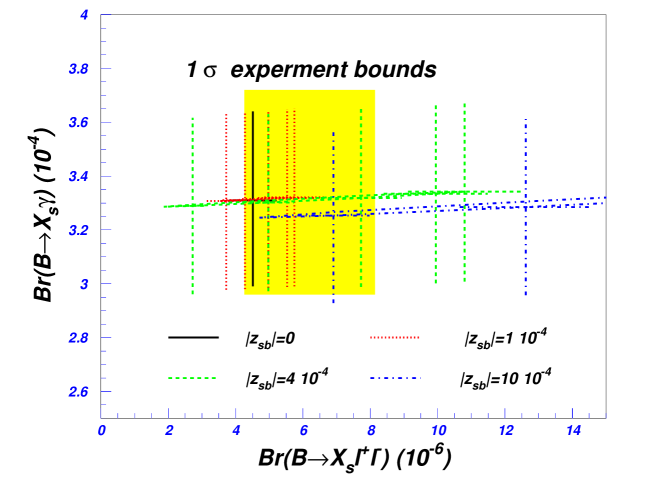
FIG. 11.: The correlation of the branching ratios of $B\to X_{s}\gamma$ and $B\to X_{s}l^{+}l^{-}$ predicted in VQM. The solid, dashed, dot and dot-dashed lines in the figure stand for different $|z_{sb}|$. Each $|z_{sb}|$ corresponds to one of the five specified $\theta=(-\pi,-\frac{3}{5}\pi,-\frac{1}{5}\pi,\frac{1}{5}\pi,\frac{3}{5}\pi)$. The experimental $1\sigma$ bounds denoted as rectangular box are taken from (1) and (141).

Fig. 11 shows correlation of the branching ratio of $B\to X_{s}\gamma$ with that of $B\to X_{s}l^{+}l^{-}$ in VQM. It is obvious from the figure that $Br(B\to X_{s}\gamma)$ is not so sensitive to the phase, which is not the case for $Br(B\to X_{s}l^{+}l^{-})$. Within the experimental bounds of $B\to X_{s}l^{+}l^{-}$ , corresponding branching ratio of $B\to X_{s}\gamma$ predicted in VQM is consistent with the experiment measurement [29]

$${\cal B}r^{ex}(B\to X_{s}\gamma)=(3.34\pm 0.38)\times 10^{-4}.$$ (141)

VI $B\to K\pi$ decays

Having established constraints on $b\to s$ FCNC from $b\to sll$ and $b\to s\gamma$, we evaluate $B\to K\pi$ decay rates. The large electroweak penguin contribution to $b\to s$ transition has been suggested in the present data of B factories. Because in VQM, the tree level FCNC may generate the electroweak penguin contribution, the purpose of this section is that with FCNC constrained by rare decays $b\to sl^{+}l^{-}$, we study whether the large electroweak penguin contribution in $B\to K\pi$ can be explained or not. The correlation between di-leptonic decay and non-leptonic decays is characteristic feature of the present model.

We start with the following effective Hamiltonian:

$$H_{eff}=\frac{4G_{F}}{\sqrt{2}}\left\{(\xi_{c}(C^{*}_{1}\bar{\cal Q}_{1}+C_{2}^{*}\bar{\cal Q}_{2})+\xi_{u}(C^{*}_{1}\bar{\cal Q}^{u}_{1}+C^{*}_{2}\bar{\cal Q}^{u}_{2})-\xi_{t}\sum_{i=1}^{10}(C^{*}_{i}\bar{\cal Q}_{i})\right\}.$$ (142)

The operators $\bar{\cal Q}_{i}$ is the charge conjugation of ${\cal Q}_{i}$ defined in (77), $\xi_{i}=K_{is}K_{ib}^{*}$, and

$$\bar{\cal Q}^{u}_{1}=(\bar{b}_{i}\gamma^{\mu}Lu_{j})(\bar{u}_{j}\gamma_{\mu}L{s}_{i}),\ \ \bar{\cal Q}^{u}_{2}=(\bar{b}_{i}\gamma^{\mu}Lu_{i})(\bar{u}_{j}\gamma_{\mu}L{s}_{j}).$$ (143)

Here we must keep the $\xi_{u}$ term because there are tree level contribution to $B\to K\pi$ decays. As seen from the effective Hamiltonian, tree-level Z FCNC generates the electroweak penguin contribution which is not suppressed by $\alpha_{em}$. In terms of isospin amplitudes, the electroweak penguin operators contribute to both $\Delta I=0$ and $\Delta I=1$ components. Because for $\Delta I=0$ amplitude, the large strong penguin contribution is expected, new physics may dominantly contribute to $\Delta I=1$ amplitudes.

Below, we estimate the $B\to K\pi$ amplitudes within the factorization approximation. The four quark operator with the flavor structure $b\to s\bar{s}{s}$ and $b\to s\bar{c}{c}$ do not contribute to the processes. We obtain

$$A(B^{+}\to K^{0}\pi^{+}) = iG_{F}\left\{\xi_{t}\left(a_{4}-\frac{a_{10}}{2}+(2a_{6}-a_{8})R^{K}\right)M^{B\pi,K}\right.$$ (145)

$$\left.+\left[\xi_{u}a_{2}-\xi_{t}\left(a_{4}+a_{10}+2(a_{6}+a_{8})R^{B}\right)\right]M^{K\pi,B}\right\},$$

$$A(B^{+}\to K^{+}\pi^{0}) = i\frac{G_{F}}{\sqrt{2}}\left\{\left[\xi_{u}\frac{a_{1}}{2}-\xi_{t}\frac{3}{4}(-a_{7}+a_{9})\right]\sqrt{2}M^{BK,\pi}\right.$$ (148)

$$\left.+\left[a_{2}\xi_{u}-\xi_{t}\left(a_{4}+a_{10}+2(a_{6}+a_{8})R^{K}\right)\right]M^{B\pi,K}\right.$$

$$\left.-\left[\xi_{u}a_{2}-\xi_{t}\left(a_{4}+a_{10}+2(a_{6}+a_{8})R^{B}\right)\right]M^{K\pi,B}\right\},$$

$$A(B^{0}\to K^{+}\pi^{-}) = iG_{F}\left\{\left[\xi_{u}a_{2}-\xi_{t}\left(a_{4}+a_{10}+2(a_{6}+a_{8})R^{K}\right)\right]M^{B\pi,K}\right.$$ (150)

$$\left.+\xi_{t}\left(a_{4}-\frac{a_{10}}{2}+(2a_{6}-a_{8})R^{B}\right)M^{K\pi,B}\right\},$$

$$A(B^{0}\to K^{0}\pi^{0}) = i\frac{G_{F}}{\sqrt{2}}\left\{\left[\xi_{u}\frac{a_{1}}{2}-\xi_{t}\frac{3}{4}(-a_{7}+a_{9})\right]\sqrt{2}M^{BK,\pi}\right.$$ (153)

$$\left.+\xi_{t}\left(a_{4}-\frac{a_{10}}{2}+(2a_{6}-a_{8})R^{K}\right)M^{B\pi,K}\right.$$

$$\left.-\xi_{t}\left(a_{4}-\frac{a_{10}}{2}+(2a_{6}-a_{8})R^{B}\right)M^{K\pi,B}\right\}$$

where $a_{2i-1}=C^{*}_{2i-1}+C^{*}_{2i}/N$, $a_{2i}=C^{*}_{2i}+C^{*}_{2i-1}/N$. And

$$R^{K} = \frac{m_{K}^{2}}{(m_{b}-m_{u})(m_{s}+m_{u})},\ \ \ R^{B}=\frac{m_{B}^{2}}{(m_{b}+m_{u})(m_{s}-m_{u})},$$ (154)

$$M^{ab,c} = f_{c}(M_{a}^{2}-m_{b}^{2})F_{0}^{a\to b}(m_{c}^{2}).$$ (155)

In derving the amplitudes, we have used

$$<\pi^{0}(p^{\prime}))|(\bar{b}u)_{V}|B^{+}(p)> = \left[(p+p^{\prime})_{\mu}-\frac{m_{B}^{2}-m_{\pi}^{2}}{q^{2}}q_{\mu}\right]F_{1}^{B^{+}\to\pi^{0}}(q^{2})+\frac{m_{B}^{2}-m_{\pi}^{2}}{q^{2}}q_{\mu}F_{0}^{B^{+}\to\pi^{0}}(q^{2}),$$ (156)

$$<K^{+}(p^{\prime}))|(\bar{b}s)_{V}|B^{+}(p)> = \left[(p+p^{\prime})_{\mu}-\frac{m_{B}^{2}-m_{K}^{2}}{q^{2}}q_{\mu}\right]F_{1}^{B\to K}(q^{2})+\frac{m_{B}^{2}-m_{K}^{2}}{q^{2}}q_{\mu}F_{0}^{B\to K}(q^{2}),$$ (157)

$$<K^{+}(-p)\pi^{0}(p^{\prime}))|(\bar{u}s)_{V}|0> = \left[(p+p^{\prime})_{\mu}-\frac{m_{K}^{2}-m_{\pi}^{2}}{q^{2}}q_{\mu}\right]F_{1}^{K\to\pi}(q^{2})+\frac{m_{K}^{2}-m_{\pi}^{2}}{q^{2}}q_{\mu}F_{0}^{K\to\pi}(q^{2}),$$ (158)

where $q=p-p^{\prime}$, and

$$<0|(\bar{s}u)_{A}|K^{+}(p_{k})>=if_{K}p_{k\mu},\ \ \ \ <0|(\bar{b}u)_{A}|B(p_{B})>=if_{B}p_{B\mu},$$ (159)

$$<K^{+}(p_{k})|(\bar{s}u)_{A}|0>=-if_{K}p_{k\mu},\ \ <\pi^{0}(p_{\pi})|(\bar{u}u-\bar{d}d)_{A}|0>=-i\sqrt{2}f_{\pi}p_{\pi\mu}.$$ (160)

It is easy to see that the isopsin relation

$$\sqrt{2}A(B^{+}\to K^{+}\pi^{0})+A(B^{+}\to K^{0}\pi^{+})=\sqrt{2}A(B^{0}\to K^{0}\pi^{0})+A(B^{0}\to K^{+}\pi^{-}).$$ (161)

Since there are many uncertainties in calculating $B\to K\pi$ such as strong phases and formfactors, instead of the branching ratios of $B\to K\pi$, it is more reasonable to use their ratios to constrain the new physics effect. In this work, we use $R_{c},\ R_{n}$ and their difference to constrain Z FCNC. $R_{c}$ and $R_{n}$ are defined as

$$R_{c} \equiv \frac{2Br(B^{+}\to K^{+}\pi^{0})+2Br(B^{-}\to K^{-}\pi^{0})}{Br(B^{+}\to K^{0}\pi^{+})+Br(B^{-}\to\bar{K}^{0}\pi^{-})},$$ (162)

$$R_{n} \equiv \frac{Br(B^{0}\to K^{+}\pi^{-})+Br(\bar{B}^{0}\to K^{-}\pi^{+})}{2Br(B^{0}\to K^{0}\pi^{0})+2Br(\bar{B}^{0}\to\bar{K}^{0}\pi^{0})}.$$ (163)

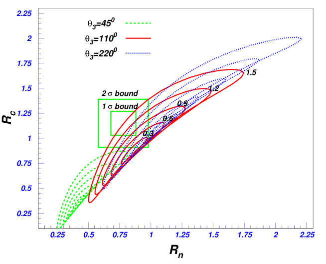
FIG. 12.: Correlation between $R_{n}$ and $R_{c}$. The dashed, solid and dotted lines denote for the phase $\theta_{3}=45^{0},110^{0},220^{0}$, respectively. For each specified phase $\theta_{3}$, the sizes of $z_{sb}$ corresponding to contours (inner to outer) are $(0.3,0.6,0.9,1.2,1.5)\times 10^{-3}$.

In our numerical calculations, we take large $N$ limit and use $f_{\pi}=132\ GeV$. Since $q^{2}=m_{K}^{2},m_{\pi}^{2}$ is rather close to the point $q^{2}=0$, we neglect the $q^{2}$ dependence in the formfactors, while $F_{0}^{B\to K}=0.33,\ F_{0}^{B\to\pi^{0}}=0.379/\sqrt{2}$. The SU(3)-breaking effects in the formfactors are also neglected. The contribution from the terms proportional to $f_{B}$ is also omitted because it works as a suppression factor $f_{B}/M_{B}$[16].

Running quark masses appear in the matrix elements of $(S-P)(S+P)$ penguin operators through the use of the motion equation. The running quark masses at $\mu\sim m_{b}=4.8\ GeV$ scale are given by

$$m_{b}(m_{b})=4.34GeV,\ \ m_{s}(m_{b})=0.09GeV,\ \ m_{u}(m_{b})=m_{d}(m_{b})=0.03GeV.$$ (164)

The NLO Wilson coefficients in NDR scheme at $m_{b}$ scale can be obtained from (96) and (105).

As discussed in Section II, the phases $\theta_{3}$ and $\theta$ are defined in (131) and are shown in Fig. 1. We can write $\theta_{3}$ as,

$$\theta_{3}\simeq-atan\left(\frac{\eta}{\rho}\right),$$ (165)

where $\eta$ and $\rho$ can be detremined from the measuerments of CP violation and mixings of $K$ and $B_{d}$ systems. By assuming that the effect of tree level FCNC on $K$ and $B_{d}$ is small, we can use the standard model values for $\eta$ and $\rho$. The allowed region of $\theta_{3}$ is:

$$100^{0}\leq\theta_{3}\leq 140^{0}.$$ (166)

If the tree level FCNC contribute to $K$ and $B_{d}$ system, the allowed region of $\theta_{3}$ can be significantly changed from Eq.(166). Therefore, in our numerical calculation, we relax this condition and scan the region for $\theta_{3}$ from $0^{0}$ to $360^{0}$. Now we can see the physics quantities are deterimined by three inputs: the size of Z FCNC coupling $|z_{sb}|$, the phases of $\theta_{3}$ and $\theta$. We plot the $R_{n}$ and $R_{c}$ correlation in Fig. 12 with three specified values of $\theta_{3}$. For given $z_{sb}$, the allowed region changes with $\theta_{3}$. For $|z_{sb}|\leq 1.5\times 10^{-3}$ and $\theta_{3}\leq 45^{0}$, no region is allowed by $R_{c}$ and $R_{n}$ experimental measurements at $2\sigma$ level. When $\theta_{3}=100^{0}\sim 120^{0}$, as shown in the figure, there are larger allowed regions.

To see this more clearly, in Fig.13 we show the dependence of $R_{c}-R_{n}$ on the phase $\theta_{3}$ with typical values $|z_{sb}|=(1.0,1.5)\times 10^{-3}$ and $\theta=(-\pi,-\frac{\pi}{2},0,\frac{\pi}{2},\pi)$. The experimental measurements [30]

$$R_{c}=1.15\pm 0.12,\ \ R_{n}=0.78\pm 0.10,\ \ R_{c}-R_{n}=0.37\pm 0.16$$ (167)

at $1\sigma$ and $2\sigma$ level are also displayed.

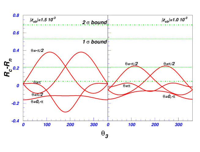
FIG. 13.: $R_{c}-R_{n}$ as a funition of the phase $\theta_{3}$.

From this figure, we note that $R_{c}-R_{n}$ is sensitive to the phase $\theta_{3}$ and $\theta$.

The constraints on the contour $(|z_{sb}|,\theta)$ from $R_{c}-R_{n}$ are shown in Fig. 14. One can see that, for $\theta_{3}=110^{0}$, $1\sigma$ experimental bounds restrict $|z_{sb}|$ and $\theta$ as $|z_{sb}|>0.9\times 10^{-3}$, $|\theta|\geq 1$. Corresponding to $2\sigma$ experimental bounds, smaller $|z_{sb}|$ is allowed as $|z_{sb}|>0.2\times 10^{-3}$.

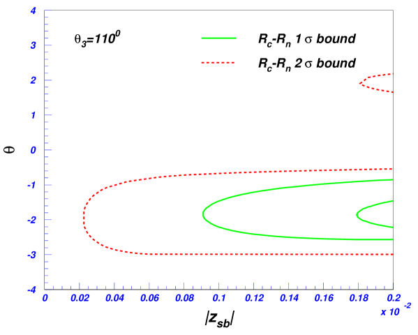
FIG. 14.: The $(|z_{sb}|,\theta)$ contour constrained by $R_{c}-R_{n}$ at $1\sigma$ and $2\sigma$ level.

Finally, we obtain the allowed regions from $R_{c}-R_{n}$ and $B\to X_{s}l^{+}l^{-}$ by varying $\theta_{3}$ as a free parameter. The bounds are shown in Fig. 15. At $1\sigma$ level, there are no overlapping region allowd from $B\to X_{s}l^{+}l^{-}$ and $B\to K\pi$. From Fig. 15, we obtain

$$0.2\times 10^{-3}<|z_{sb}|<1.2\times 10^{-3},\ (95\%\ C.\ L.)$$ (168)

where large phase $|\theta|$ is favored. Now we would like to point out that if $\theta_{3}$ is in the region of $[100^{0},140^{0}]$, only the region with negative phase $\theta$ in Fig. 15 is allowed.

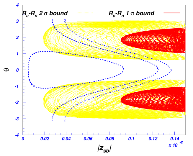
FIG. 15.: The $(|z_{sb}|,\theta)$ contour constrained by combination of $B\to X_{s}l^{+}l^{-}$ and $B\to K\pi$ at $1\sigma$ and $2\sigma$ level. The solid and dotted lines correspond to $1\sigma$ and $2\sigma$ bounds from $R_{c}-R_{n}$, respectively. The dash-dotted line and dashed lines correspond to $2\sigma$ and $1\sigma$ bounds from $B\to X_{s}l^{+}l^{-}$. The allowed region with $\theta>0$ corresponds to $180^{0}<\theta_{3}<360^{0}$ whereas the allowed region with $\theta<0$ corresponds to $0^{0}<\theta_{3}<180^{0}$.

VII Conclusions

In this work, we have studied the new physics effects on the B meson decays $B\to X_{s}\gamma,B\to X_{s}\ell^{+}\ell^{-}$ and $B\to K\pi$ in the Vectorlike Quark Model. The QCD running effect from the mass of the down-type vector quark $D$ to weak scale has been taken into account. We extracted rather stringent constraints on the size of the tree level Z FCNC coupling and its CP violating phase from $B\to X_{s}\ell^{+}\ell^{-}$. Within the bounds, we investigated various observables such as FB asymmetry of $b\to sl^{+}l^{-}$, the decay rates of $B\to X_{s}\gamma$ and $B\to K\pi$. We found that the zero crossing point of FB asymmetry $s_{0}$ of $B\to X_{s}l^{+}l^{-}$ is very sensitive to both the size and phase of $z_{sb}$ and can be useful in probing the new physics, and both experimental measurements for $B\to X_{s}l^{+}l^{-}$ and $B\to K\pi$ decays can be explained within the framework of vector-like quark model. The upper bound on the size of $Z$ FCNC comes from $B\to X_{s}l^{+}l^{-}$ , while the lower bound, from $B\to K\pi$ decays. Considering that the B factories such as BaBar and Belle are running, measurements for inclusive and exclusive B decays with high precision are expected. Therefore, the VQM will be tested in near future.

A

In this appendix, we present all anomalous dimension matrices needed in solving the Wilson coefficients.

(1) For the mixings of operators $Q^{H}_{LR},\ R^{1,H}_{L},\ R^{2,H}_{L}$, we obtain

$$\gamma=\left(\begin{array}[]{ccc}7&0&0\\ 0&7&0\\ 0&0&7\\ \end{array}\right).$$ (A4)

We also obtain the same matrix for $Q^{\chi}_{LR},\ R^{1,\chi}_{L},\ R^{2,\chi}_{L}$ as Eq.(A4). For the mixings among the operators $O_{LR}^{i}\ (i=1,2,3)$ and $P_{L}^{1,A},\ P_{L}^{2}$, we obtain the following result:

$$\gamma=\frac{g_{s}^{2}}{8\pi^{2}}\left(\begin{array}[]{cccccccc}\frac{20}{3}&1&-2&0&0&0&0&0\\ -8&\frac{2}{3}&\frac{4}{3}&0&0&0&0&0\\ 0&0&\frac{16}{3}&0&0&0&0&0\\ 6&2&-1&\frac{2}{3}&2&-2&-2&0\\ 4&\frac{3}{2}&0&-\frac{113}{36}&\frac{137}{18}&-\frac{113}{36}&-\frac{4}{3}&\frac{9}{4}\\ 2&1&1&-2&2&\frac{2}{3}&-2&0\\ 0&\frac{1}{2}&2&-\frac{113}{36}&\frac{89}{18}&-\frac{113}{36}&\frac{4}{3}&\frac{9}{4}\\ \end{array}\right),$$ (A12)

which is in agreement with Ref.[22].

(2) The $10\times 10$ one-loop anomalous dimension matrix among ${\cal Q}_{1-10}$ is given by [25]:

$$\gamma^{(0)}=\left(\begin{array}[]{cccccccccc}-2&6&0&0&0&0&0&0&0&0\\ 6&-2&\frac{-2}{9}&\frac{2}{3}&\frac{-2}{9}&\frac{2}{3}&0&0&&0\\ 0&0&\frac{-22}{9}&\frac{22}{3}&\frac{-4}{9}&\frac{4}{3}&0&0&0&0\\ 0&0&6-\frac{2f}{9}&-2+\frac{2f}{3}&\frac{-2f}{9}&\frac{2f}{3}&0&0&&0\\ 0&0&0&0&2&-6&0&0&0&0\\ 0&0&-\frac{2f}{9}&\frac{2f}{3}&\frac{-2f}{9}&-16+\frac{2f}{3}&0&0&0&0\\ 0&0&0&0&0&0&2&-6&0&0\\ 0&0&\frac{-2(u-d/2)}{9}&\frac{2(u-d/2)}{3}&\frac{-2(u-d/2)}{9}&\frac{2(u-d/2)}{3}&0&-16&0&0\\ 0&0&\frac{2}{9}&\frac{-2}{3}&\frac{2}{9}&\frac{-2}{3}&0&0&-2&6\\ 0&0&\frac{-2(u-d/2)}{9}&\frac{2(u-d/2)}{3}&\frac{-2(u-d/2)}{9}&\frac{2(u-d/2)}{3}&0&0&6&-2\\ \end{array}\right)$$ (A23)

where the color number $N=3$ is used. For $b\to sl^{+}l^{-}$, $f=u+d,\ u=2,d=3$. $\gamma^{(0)}$ is scheme independent.

In NDR scheme the $10\times 10$ two-loop anomalous dimension matrix among the ${\cal Q}_{1-10}$ is given by

$$\gamma^{NDR,(1)}=\begin{array}[]{c}\left(\begin{array}[]{ccccc}\frac{-21}{2}-\frac{2f}{9}&\frac{7}{2}+\frac{2f}{3}&\frac{79}{9}&\frac{-7}{3}&\frac{-65}{9}\\ \frac{7}{2}+\frac{2f}{3}&\frac{-21}{2}-\frac{2f}{9}&\frac{-202}{243}&\frac{1354}{81}&\frac{-1192}{243}\\ 0&0&\frac{-5911}{486}+\frac{71f}{9}&\frac{5983}{162}+\frac{f}{3}&\frac{-2384}{243}-\frac{71f}{9}\\ 0&0&\frac{379}{18}+\frac{56f}{243}&\frac{-91}{6}+\frac{808f}{81}&\frac{-130}{9}-\frac{502f}{243}\\ 0&0&\frac{-61f}{9}&\frac{-11f}{3}&\frac{71}{3}+\frac{61f}{9}\\ 0&0&\frac{-682f}{243}&\frac{106f}{81}&\frac{-225}{2}+\frac{1676f}{243}\\ 0&0&\frac{-61(u-d/2)}{9}&\frac{-11(u-d/2)}{3}&\frac{83(u-d/2)}{9}\\ 0&0&\frac{-682(u-d/2)}{243}&\frac{106(u-d/2)}{81}&\frac{704(u-d/2)}{243}\\ 0&0&\frac{202}{243}+\frac{73(u-d/2)}{9}&\frac{-1354}{81}-\frac{(u-d/2)}{3}&\frac{1192}{243}-\frac{71(u-d/2)}{9}\\ 0&0&\frac{-79}{9}-\frac{106(u-d/2)}{243}&\frac{7}{3}+\frac{826(u-d/2)}{81}&\frac{65}{9}-\frac{502(u-d/2)}{243}\\ \end{array}\right.\\ \left.\begin{array}[]{ccccc}-\frac{7}{3}&0&0&0&0\\ \frac{904}{81}&0&0&0&0\\ \frac{1808}{81}-\frac{f}{3}&0&0&0&0\\ \frac{-14}{3}+\frac{646f}{81}&0&0&0&0\\ -99+\frac{11f}{3}&0&0&0&0\\ \frac{-1343}{6}+\frac{1348f}{81}&0&0&0&0\\ \frac{-11(u-d/2)}{3}&\frac{71}{3}-\frac{22f}{9}&-99+\frac{22f}{3}&0&0\\ \frac{736(u-d/2)}{81}&\frac{-225}{3}+4f&-\frac{1343}{6}+\frac{68f}{9}&0&0\\ -\frac{904}{81}-\frac{(u-d/2)}{3}&0&0&\frac{-21}{2}-\frac{2f}{9}&\frac{7}{2}+\frac{2f}{3}\\ \frac{7}{3}+\frac{646(u-d/2)}{81}&0&0&\frac{7}{2}+\frac{2f}{3}&\frac{-21}{2}-\frac{2f}{9}\\ \end{array}\right).\end{array}$$ (A46)

(3) The mixing entries among ${\cal Q}_{7\gamma,8G}$ and ${\cal Q}_{1-10}$ are follows:

$$\gamma_{\gamma\gamma}=\frac{32}{3},\ \ \gamma_{G\gamma}=-\frac{32}{9},\ \ \gamma_{GG}=\frac{28}{3}.$$ (A47)

In HV scheme, the entries of $\beta_{\gamma,G}^{7-10}$ can be extracted from $\beta_{\gamma,G}^{3-6}$ [23] by substituting

$$1\to\frac{3}{2}e_{d},\ \ u\to\frac{3}{2}e_{u}u,\ \ d\to\frac{3}{2}e_{d}d,$$ (A48)

and thus, they are given by

$$\beta_{\gamma} = \left(0,\frac{416}{81},-\frac{464}{81},(\frac{416}{81}u-\frac{232}{81}d),\frac{32}{9},-(\frac{448}{81}u-\frac{200}{81}d),-\frac{16}{9},-(\frac{448}{81}u^{2}+\frac{100}{81}d^{2}),\frac{232}{81},-(\frac{416}{81}u^{2}-\frac{116}{81}d^{2})\right),$$ (A49)

$$\beta_{G} = \left(3,\frac{70}{27},\frac{140}{27}+3f,6+\frac{70}{27}f,-\frac{14}{3}-3f,-4-\frac{119}{27}f,\frac{7}{3}-3(u-\frac{d}{2}),2-\frac{119(u-d/2)}{27},\right.$$ (A51)

$$\left.-\frac{70}{27}+3(u-\frac{d}{2}),-3+\frac{70(u-d/2)}{27}\right),$$

(4) The mixing entries among ${\cal C}_{9}$ and ${\cal Q}_{1-10}$ are follows [25] with same substitution in (A48):

$$\gamma^{(0)}_{i,11} = \left(-\frac{16}{3},\frac{-16}{9},\frac{-16}{3}(u-\frac{d}{2}-\frac{1}{3}),\frac{-16}{9}(u-\frac{d}{2}-3),\frac{-16}{3}(u-\frac{d}{2}),\right.$$ (A53)

$$\left.-\frac{16}{9}(u-\frac{d}{2}),-(\frac{16}{3}u^{2}+\frac{4}{3}d^{2}),-(\frac{16}{9}u^{2}+\frac{4}{9}d^{2}),-(\frac{16}{3}u^{2}+\frac{4}{3}d^{2}+\frac{8}{9}),-(\frac{16}{9}u^{2}+\frac{4}{9}d^{2}+\frac{8}{3})\right),$$

$$\gamma^{NDR,(1)}_{i,11} = \left(-\frac{64}{3},\frac{1600}{243},-\frac{3712}{243}-\frac{64(u-d/2)}{3},\frac{64}{3}-\left(\frac{2240}{243}u+\frac{512}{243}d\right),-\frac{64(u-d/2)}{3},\frac{3520}{243}u-\frac{3392}{243}d,\right.$$ (A55)

$$\left.-(\frac{64}{3}u^{2}+\frac{16}{3}d^{2}),(\frac{3520}{243}u^{2}+\frac{1696}{243}d^{2}),\frac{1856}{243}-(\frac{64}{3}u^{2}+\frac{16}{3}d^{2}),-\frac{32}{3}-(\frac{2240}{81}u^{2}-\frac{256}{243}d^{2})\right),$$

$$\gamma^{(0)}_{11,11} = -2\beta_{0},\ \ \gamma^{NDR,(1)}_{11,11}=-2\beta_{1},$$ (A56)

where $\beta_{0}=11-2f/3,\beta_{1}=102-38f/3$.

B

Some one-loop functions needed in our calculations are follows.

(1) For the calculation of the initial values of ${\widetilde{C}}_{1-8}$ and ${\cal C}_{9,10}$ at $m_{W}$ scale:

$$A(x) = -\frac{8x^{3}+5x^{2}-7x}{12(1-x_{t})^{3}}+\frac{x^{2}(2-3x)}{2(1-x)^{4}}\ln x,$$ (B1)

$$B(x) = -\frac{x}{4(x-1)}+\frac{x}{4(x-1)^{2}}\ln x,$$ (B2)

$$C(x) = \frac{x^{2}-6x}{8(x-1)}+\frac{3x^{2}+2x}{8(x-1)^{2}}\ln x,$$ (B3)

$$D(x) = -\frac{19x^{3}-25x^{2}}{36(x-1)^{3}}-\frac{3x^{4}-30x^{3}+54x^{2}-32x+8}{18(x-1)^{4}}\ln x,$$ (B4)

$$E(x) = -\frac{2}{3}\ln x+\frac{x(18-11x-x^{2})}{12(1-x^{3})},$$ (B5)

$$F(x) = -\frac{x^{3}-5x^{2}+2x}{4(1-x)^{3}}+\frac{3x^{2}}{2(1-x)^{4}}\ln x.$$ (B6)

(2) For the calculation of one-loop diagrams with down-type vector quark $D$:

$$f_{D}^{Z}(x) = -\frac{5x^{2}+5x-4}{72(x-1)^{3}}+\frac{x(2x-1)}{12(x-1)^{4}}\ln x,$$ (B7)

$$f_{D}^{H}(x) = -e_{d}x\left[\frac{7x^{2}-29x+16}{48(x-1)^{3}}+\frac{3x-2}{8(x-1)^{4}}\ln x\right],$$ (B8)

$$f_{D}^{\chi}(x) = e_{d}x\left[\frac{5x^{2}-19x+20}{48(x-1)^{3}}+\frac{x-2}{8(x-1)^{4}}\ln x\right],$$ (B9)

REFERENCES

- [1] Super B factory report, A.G. Akeroyd, et. al., hep-ex/0406071.
- [2] B. Aubert et al. [BABAR Collaboration], hep-ex/0207074; hep-ex/0207076.
- [3] CELO Collaboration, S. Chen et al., Phys. Rev.o Lett.87 (2001) 251807.
- [4] [ALEPH Collaboration], Phys. Lett. B428 (1998) 189.
- [5] K. Chetyrkin, M. Misiak and M. Munz, Phys. Lett. B400 (1997) 206; B425 (1998) 414 (E).
- [6] A.J. Buras, A. Kwiatkowaki and N. Pott, Phys. Lett. B414 (1997) 157; B434 (1998) 459 (E).
- [7] [BABAR Collaboration], hep-ph/0308016.
- [8] [Belle Collaboration], Phys. Rev. Lett.90 (2003) 021801.
- [9] M. Nakao, talk at the XXI Int. Symp. on Lepton and Photon Interactions at High Energies, August 2003, Fermilab, USA.
- [10] L.T. Handoko and T. Morozumi, Modern Phys. Lett. A10 (1995) 309.
- [11] C.-H. V. Chang, D. Chang and W.-Y. Keung, Phys. Rev. D61 (2000) 053007.
- [12] M.R. Ahmady, M. Nagashma and A. Sugamoto, Phys. Rev. D64 (2001) 054011.
- [13] G. Barenboim, F.J. Botella and O. Vives, Nucl. Phys. B613 (2001) 613; D. Hawkins and D. Silverman, Phys. Rev. D66 (2002) 016008; T. Yanir, JHEP 0206 (2002) 044.
- [14] J.A. Aguilar-Saavedra, hep-ph/0210112.
- [15] Y. Grossmann, M. Neubert and A. Kagan, JHEP 9910,(1999) 029 ; M. Gronau, D. Pirjol and T.-M. Yan, Phys. Rev. D60, (1999) 034021 ; R. Fleischer and J. Matias, Phys. Rev. D61, (2000) 074004; R. Fleischer and J. Matias, Phys. Rev. D66, (2002) 054009.
- [16] T. Yoshikawa, Phys. Rev. D68 (2003) 054023 ; S. Mishima and T. Yoshikawa, hep-ph/0408090.
- [17] M. Gronau and J.L. Rosner, Phys. Lett. B572,(2003) 43 ; C.-W. Chiang, M. Gronau, J.L. Rosner and D.A. Suprun, hep-ph/0404073.
- [18] A.J. Buras, R. Fleischer, S. Recksiegel and F. Schwab, Eur. Phys. J. C32, (2003) 45; A.J. Buras, R. Fleischer, S. Recksiegel and F. Schwab, Phys. Rev. Lett. 92, (2004) 101804; A.J. Buras, R. Fleischer, S. Recksiegel and F. Schwab, hep-ph/0402112 ; A.J. Buras, hep-ph/0402191 ; A.J. Buras, F. Schwab and S. Uhlig, hep-ph/0405132.
- [19] Y.-Y. Charng and H.-n. Li, hep-ph/0308257.
- [20] G.C. Branco, T. Morozumi, P.A. Parada and M.N. Rebelo, Phys. Rev. D48 (1993) 1167.
- [21] P. Cho and B. Grinstein, Nucl. Phys. B365 (1991) 279.
- [22] C.S. Gao, J.L. Hu, C.D. Lü and Z.M Qiu, Phys. Rev. D52 (1995) 3978.
- [23] M. Ciuchini et. al., Phys. Lett. B334 (1994) 137.
- [24] A.J. Buras et al., Nucl. Phys. B370 (1992) 69.
- [25] A.J. Buras, M. Misiak, M. Munz and S. Pokorski Nucl. Phys. B424 (1994) 374.
- [26] M. Misiak, Nucl. Phys. B393 (1993) 23, Erratum, Nucl. Phys. B439 (1995) 461; A.J. Buras, Phys. Rev. D52 (1995) 186.
- [27] A. Ali, G. Hiller, L.I. Handoko and T. Morozumi, Phys. Rev. D55 (1997) 4105.
- [28] N. Cabibbo and L. Maiani, Phys. Lett. B79 (1978) 109.
- [29] C.P. Jessop, preprint SLAC-PUB-9610, November 2002.
- [30] Heavy Flavor Averaging Group, (before 2004 summer), http://www.slac.stanford.edu/xorg/hfag/