The Čerenkov effect in Lorentz-violating vacua

Abstract

The emission of electromagnetic radiation by charges moving uniformly in a Lorentz-violating vacuum is studied. The analysis is performed within the classical Maxwell–Chern–Simons limit of the Standard-Model Extension (SME) and confirms the possibility of a Čerenkov-type effect. In this context, various properties of Čerenkov radiation including the rate, polarization, and propagation features, are discussed, and the back-reaction on the charge is investigated. An interpretation of this effect supplementing the conventional one is given. The emerging physical picture leads to a universal methodology for studying the Čerenkov effect in more general situations.

I Introduction

Recent years have witnessed substantial progress in quantum-gravity phenomenology: minute Lorentz and CPT violations have been identified as promising candidate signatures for Planck-scale physics cpt01 . At presently attainable energies, such signatures are described by an effective-field-theory framework called the Standard-Model Extension (SME) ck ; grav ; kl01 . The violation parameters in the SME can arise in various underlying contexts, such as strings kps , spacetime-foam approaches lqg ; kp03 ; klink , noncommutative geometry ncft , varying scalars vc ; aclm , random-dynamics models rd , multiverses mv , and brane-world scenarios bws . The flat-spacetime limit of the SME has provided the basis for numerous analyses of Lorentz breaking including ones involving mesons hadronexpt ; kpo ; hadronth ; ak , baryons ccexpt ; spaceexpt ; cane , electrons eexpt ; eexpt2 ; eexpt3 , photons cfj ; photonexpt ; photonth ; cavexpt ; km , muons muons , and the Higgs sector higgs ; neutrino-oscillation experiments offer the potential for discovery ck ; neutrinos ; nulong .

A Lorentz-violating vacuum acts in many respects like a nontrivial medium. For example, one expects the electrodynamics limit of the SME to possess features similar to those of ordinary electrodynamics in macroscopic media ck . Indeed, changes in the propagation of electromagnetic waves, such as modified group velocities and birefringence, have been predicted and used to place tight bounds on Lorentz violation cfj ; km . Another conventional feature in macroscopic media, which is associated with fast charges, is the emission of Čerenkov light cerh ; cerexp ; cerclass ; cerquant . A similar mechanism, radiation of photons from charged particles in certain Lorentz-breaking vacua, has been suggested in the literature vcr . Because of the close analogy to the conventional Čerenkov case, this mechanism is sometimes called the “vacuum Čerenkov effect.” This idea is widely employed in cosmic-ray analyses of Lorentz violation vcrtests . The first complete theoretical discussion of the vacuum Čerenkov effect—including a general methodology for extracting radiation rates in classical situations—has been performed in Ref. lp04 . This methodology has subsequently also been employed in a non-electromagnetic context aclt04 .

The present work extends our previous analysis lp04 : we give a more detailed derivation of the results and investigate additional important aspects of vacuum Čerenkov radiation. More specifically, we provide an intuitive physical picture for the effect, discuss the polarization and propagation properties of the emitted light, and study the back-reaction on the charge. Our analysis is performed within the classical Maxwell–Chern–Simons limit of the SME’s electrodynamics sector, but we expect our methodology and results to be applicable in more general situations as well.

A more refined understanding of the Čerenkov effect in conventional physics provides an additional motivation for our study. Recent observations at CERN involving high-energy lead ions cern and experiments in exotic condensed-matter systems cms have revived the interest in the subject certheo . In particular, these experimental and theoretical investigations have found evidence for unconventional kinematical radiation conditions, backward photon emission, and backward-pointing radiation cones in such contexts. Since our methodology differs from the conventional one in several respects, it yields additional insight into the ordinary Čerenkov effect as well. For example, the presence of a fully relativistic Lagrangian, which incorporates dispersion, makes it feasible to work in the charge’s rest frame simplifying the calculation. In particular, the exact emission rate for point particles carrying an electromagnetic charge and a magnetic moment can be determined without the explicit field solutions.

The outline of this paper is as follows. Section II reviews some basics of the Maxwell–Chern–Simons model. In Sec. III, we set up the problem in a model-independent way and extract the general condition for the emission of Čerenkov light. The concrete calculation of the radiation rate in the Maxwell–Chern–Simons model is performed in Sec. IV. Section V discusses the back-reaction on the charge. In Sec. VI, a complementary, purely kinematical approach for estimating radiation rates is presented. We comment briefly on experimental implications in Sec. VII. The conclusions are contained in Sec. VIII. Appendix A provides supplementary material about the plane-wave dispersion relation. The wave polarizations are briefly discussed in Appendix B. In Appendix C, we determine the radiation rate for a charged magnetic dipole.

II Basics

The renormalizable gauge-invariant photon sector of the SME contains a CPT-odd and a CPT-even operator parametrized by $(k_{AF})^{\mu}$ and $(k_{F})^{\mu\nu\rho\sigma}$, respectively. Many components of these parameters are strongly constrained by astrophysical spectropolarimetry photonexpt . However, further investigations remain to be of great interest both for a better understanding of massless Lorentz-violating fields and for the potential of complementary tighter bounds. In the present work, we consider the Chern–Simons-type $(k_{AF})^{\mu}$ modification. The Maxwell–Chern–Simons model resulting from such a modification has been studied extensively in the literature cfj ; klink ; mcsclass ; mcsquant . The $(k_{AF})^{\mu}$ parameter has mass dimensions, which leads to the more interesting case of nontrivial dispersion. Note also that many characteristics of Čerenkov radiation, such as rates and energy fluxes, require at least one dimensionful model parameter. With only a dimensionless $(k_{F})^{\mu\nu\rho\sigma}$, the usual approach to the Čerenkov effect involving an external nondynamical point source might be problematic for obtaining a finite rate.

In natural units $c=\hbar=1$, the Maxwell–Chern–Simons Lagrangian in the presence of external sources $j^{\mu}$ is

$${\cal L}_{\rm MCS}=-{{1}\over{4}}F_{\mu\nu}F^{\mu\nu}+(k_{AF})_{\mu}A_{\nu}\tilde{F}^{\mu\nu}-A_{\mu}j^{\mu},$$ (1)

where $F_{\mu\nu}=\partial_{\mu}A_{\nu}-\partial_{\nu}A_{\mu}$ denotes the conventional electromagnetic field-strength tensor and $\tilde{F}^{\mu\nu}={\textstyle{1\over 2}}\varepsilon^{\mu\nu\rho\sigma}F_{\rho\sigma}$ its dual, as usual. Since we take $(k_{F})^{\mu\nu\rho\sigma}=0$, we can omit the subscript $AF$ of the Lorentz- and CPT-violating $(k_{AF})^{\mu}$ parameter and set $(k_{AF})^{\mu}\equiv k^{\mu}=(k^{0},\vec{k})$. In this work, $k^{\mu}$ must not be confused with the traditional notation of Fourier momenta. A nondynamical fixed $k^{\mu}$ determines a special direction in spacetime. For example, certain features of plane waves propagating along $\vec{k}$ might differ from those of waves perpendicular to $\vec{k}$. Thus, particle Lorentz symmetry is violated ck ; rl03 . However, note that the Lagrangian (1) transforms as a scalar under rotations and Lorentz boosts of the reference frame. This coordinate independence remains a fundamental principle regardless of particle Lorentz breaking. It guarantees that the physics is left unaffected by an observer’s choice of coordinates and is therefore also called observer Lorentz symmetry ck ; rl03 . This principle is essential for our discussion in Sec. III.

The Lagrangian (1) yields the following equations of motion for the potentials $A^{\mu}=(A^{0},\vec{A})$:

$$\left(\Box\eta^{\mu\nu}-\partial^{\mu}\partial^{\nu}-2\varepsilon^{\mu\nu\rho\sigma}k_{\rho}\partial_{\sigma}\right)A_{\nu}=j^{\mu}.$$ (2)

As in conventional electrodynamics, current conservation $\partial_{\mu}j^{\mu}=0$ emerges as a compatibility requirement. For completeness, we also give the modified Coulomb and Ampère laws contained in Eq. (2):

$$\vec{\nabla}\!\cdot\!\vec{E}-2\vec{k}\!\hskip 0.8pt\cdot\!\vec{B} = \rho,$$

$$-\dot{\vec{E}}+\vec{\nabla}\!\times\!\vec{B}-2k_{0}\vec{B}+2\vec{k}\!\times\!\vec{E} = \hskip 1.5pt\vec{\textit{\j}}\hskip 1.0pt.$$ (3)

The homogeneous Maxwell equations remain unchanged because the field–potential relationship is the usual one. The potential $A^{0}$ is nondynamical, and gauge symmetry eliminates another component of $A^{\mu}$, so that Eq. (2) contains two independent degrees of freedom paralleling the conventional Maxwell case. To fix a gauge, any of the usual conditions on $A^{\mu}$, such as Lorentz or Coulomb gauge, can be imposed. Note, however, that there are some differences between conventional electrodynamics and the present model regarding the equivalence of certain gauge choices. A more detailed discussion of the degrees of freedom and the gauge-fixing process is contained in the second paper of Ref. ck .

The tensor given by

$$\Theta^{\mu\nu}=-F^{\mu\alpha}F^{\nu}{}_{\!\alpha}+{{1}\over{4}}\eta^{\mu\nu}F^{\alpha\beta}F_{\alpha\beta}-k^{\nu}\tilde{F}^{\mu\alpha}A_{\alpha}$$ (4)

is associated with the energy and momentum stored in our modified electromagnetic fields. Here, $\eta^{\mu\nu}$ denotes the usual metric with signature $-2$ in flat Minkowski space. Although the energy–momentum tensor is gauge dependent, it changes only by a 3-gradient under a gauge transformation $A^{\mu}\rightarrow A^{\mu}+\partial^{\mu}\Lambda$, so that the total 4-momentum obtained by a spatial integration remains unaffected. More generally, the action—and therefore the physics—is gauge invariant fn4 . As opposed to the conventional case, $\Theta^{\mu\nu}$ cannot be symmetrized because its antisymmetric part is no longer a total derivative. It follows from the equations of motion (2) that the energy–momentum tensor (4) obeys

$$\partial_{\mu}\Theta^{\mu\nu}=j_{\mu}F^{\mu\nu}.$$ (5)

The presence of sources $j^{\mu}\neq 0$ implies that $\Theta^{\mu\nu}$ is not conserved, as expected fn1 .

To find solutions of the equations of motion (2) one can employ standard Fourier methods. The modified Maxwell operator appearing in parentheses in Eq. (2) is singular, as in the conventional case. This can be verified in Fourier space, where the corresponding Minkowski matrix fails to be invertible. To circumvent this obstacle, we can proceed in Lorentz gauge, as usual. Then, Eq. (2) takes the form

$$\left(-p^{2}\eta_{\nu\lambda}+2i\varepsilon_{\nu\lambda\rho\sigma}k^{\rho}p^{\sigma}\right)\hat{A\>\,}\!\!^{\lambda}=\textit{\^{\j}}\hskip 0.5pt_{\nu}$$ (6)

in $p^{\mu}$ Fourier space. Here, the caret denotes the four-dimensional Fourier transform, and the dependence of $\hat{A\>\,}\!\!_{\nu}$ and $\textit{\^{\j}}\hskip 0.5pt_{\nu}$ on the wave 4-vector $p^{\mu}=(\omega,\vec{p}\hskip 1.0pt)$ is understood. Contraction of Eq. (6) with the tensor

$$\hat{G}^{\mu\nu}\equiv-{{p^{2}\eta^{\mu\nu}+2i\varepsilon^{\mu\nu\rho\sigma}k_{\rho}p_{\sigma}+4k^{\mu}k^{\nu}}\over{p^{4}+4p^{2}k^{2}-4(p\!\hskip 0.8pt\cdot\!k)^{2}}}+4\hat{G}^{\mu\nu}_{0},$$ (7)

where

$$\hat{G}^{\mu\nu}_{0}\equiv{{(p\!\hskip 0.8pt\cdot\!k)(p^{\mu}k^{\nu}+k^{\mu}p^{\nu})-k^{2}p^{\mu}p^{\nu}}\over{\big{[}p^{4}+4p^{2}k^{2}-4(p\!\hskip 0.8pt\cdot\!k)^{2}\big{]}p^{2}}},$$ (8)

yields the Fourier-space solution $\hat{A\>\,}\!\!^{\mu}=\hat{G}^{\mu\nu}\textit{\^{\j}}\hskip 0.5pt_{\nu}$ of the equations of motion. This establishes that $\hat{G}^{\mu\nu}(p^{\mu})$ is a momentum-space Green function for Eq. (6). Transformation to position space now gives the general solutions $A^{\mu}(x)$ of Eq. (2):

$$A^{\mu}(x)=A^{\mu}_{0}(x)+\int\limits_{C_{\omega}}{{d^{4}p}\over{(2\pi)^{4}}}\;\hat{G}^{\mu\nu}\textit{\^{\j}}\hskip 0.5pt_{\nu}\exp(-ip\!\hskip 0.8pt\cdot\!x),$$ (9)

where $x^{\mu}=(t,\vec{r}\hskip 1.0pt)$ denotes the spacetime-position vector and $A^{\mu}_{0}(x)$ satisfies Eq. (2) in the absence of sources. As in the conventional case, the freedom in choosing $A^{\mu}_{0}(x)$ and the $\omega$-integration contour $C_{\omega}$ can be used to satisfy boundary conditions.

The poles of the integrand in Eq. (9) determine the plane-wave dispersion relation. With Def. (7), we obtain

$$p^{4}+4p^{2}k^{2}-4(p\!\hskip 0.8pt\cdot\!k)^{2}=0.$$ (10)

This equation yields the wave frequency $\omega$ for a given wave 3-vector $\vec{p}$. It is known that this dispersion relation admits spacelike wave 4-vectors for any nontrivial value of $k^{\mu}$ klink . Such vectors will turn out to be the driving entity for Čerenkov radiation. The roots of the dispersion relation (10) are discussed in Appendix A. Note that the $\hat{G}^{\mu\nu}_{0}$ term exhibits additional poles at $p^{2}=0$. However, this piece of the Green function does not contribute to the physical fields: upon contraction of $\hat{G}^{\mu\nu}_{0}$ with $\textit{\^{\j}}\hskip 0.5pt_{\nu}$, terms with $p\cdot\textit{\^{\j}}\hskip 0.5pt$ vanish due to current conservation. The remaining term in Eq. (8), proportional to $p^{\mu}$, amounts to a total derivative and is therefore pure gauge.

The contour plays a pivotal role in our study. We choose the usual retarded boundary conditions, so that $C_{\omega}$ passes above all poles on the real-$\omega$ axis. However, for timelike $k^{\mu}$ Eq. (10) determines poles both in the lower and in the upper half plane. Thus, the Green function for timelike $k^{\mu}$ will in general be nonzero also in the acausal region $t<0$. This is consistent with earlier findings of microcausality violations in the presence of a timelike $k^{\mu}$ cfj ; klink . We remark that the Lorentz-violating modifications to the conventional Maxwell operator leave unchanged the structure of the highest-derivative terms and are thus mild enough to maintain hyperbolicity. Therefore, the more general Fourier–Laplace method can be employed to define a retarded Green function in the timelike-$k^{\mu}$ situation at the cost of introducing exponentially growing solutions. We disregard this possibility here and focus on the spacelike- and lightlike-$k^{\mu}$ cases.

In the present context, it is convenient to implement the definition of the contour by shifting the poles at real $\omega$ into the lower half plane. To this end, we replace $\omega\rightarrow\omega+i\varepsilon$ in the denominator of the integrand in Eq. (9). Here, $\varepsilon$ is an infinitesimal positive parameter that is taken to approach zero after the integration. This prescription is reminiscent of the Fourier–Laplace approach, where $\varepsilon$ could in general also be finite. To ensure compatibility of the Fourier–Laplace transform with the present Fourier methods in the limit $\varepsilon\rightarrow+0$, the prescription $\omega\rightarrow\omega+i\varepsilon$ must be implemented in each $p$ of the denominator.

III Conceptual considerations

Observer invariance of the Lagrangian (1) implies that the presence or absence of vacuum Čerenkov radiation is independent of the coordinate system. We can therefore proceed in a rest frame of the charge fn2 . In such a frame, many conceptual issues become more transparent and the calculations are simpler. For instance, a condition for radiation is that at least part of the energy–momentum flux associated with the fields of the charge must escape to spatial infinity $|\vec{r}\hskip 1.0pt|=r\to\infty$. Thus, the modified energy–momentum tensor (4) must contain pieces that do not fall off faster than $r^{-2}$. Excluding a logarithmic behavior of the potentials, both $A^{\mu}$ and $F^{\mu\nu}$ should then exhibit an asymptotic $r^{-1}$ dependence.

To some extent, this parallels the case of a local time-dependent 4-current distribution in conventional electrodynamics. For example, the fields of a rotating electric dipole behave like $r^{-1}\cos(\omega t-|\vec{p}\hskip 1.0pt|r+\varphi)$ at large distances. In this example, $\omega$ corresponds to the rotation frequency, and $\varphi$ denotes a field-specific phase Jackson . Note that the fields oscillate both with time and with distance. In the present case, however, we require the 4-current of a particle at rest to be stationary leading to time-independent fields. Radiation can then occur in the presence of terms oscillating with distance only. Such terms are absent in ordinary vacuum electrodynamics. In the present context, we must therefore investigate whether the Lorentz-violating modification of the fields associated with a particle at rest can exhibit such an oscillatory behavior.

As a consequence of the presumed time independence in the particle’s rest frame, the four-dimensional $p^{\mu}$ Fourier transform of the 4-current is $\textit{\^{\j}}\hskip 1.0pt^{\mu}(p^{\mu})=2\pi\delta(\omega)\textit{\~{\j}}\hskip 1.0pt^{\mu}(\vec{p}\hskip 1.0pt)$, where the tilde denotes the three-dimensional $\vec{p}$ Fourier transform. Then, the charge’s fields are generally determined by the inverse Fourier transform of an expression containing $1/D(0,\vec{p}\hskip 1.0pt)$, where $D(\omega,\vec{p}\hskip 1.0pt)=0$ is the plane-wave dispersion relation. For example, in the present Maxwell–Chern–Simons model Eq. (9) leads (up to homogeneous solutions) to the fields

$$A^{\mu}(\vec{r}\hskip 1.0pt)=\int{{d^{3}\vec{p}}\over{(2\pi)^{3}}}\;{{N^{\mu\nu}(\vec{p}\hskip 1.0pt)\textit{\~{\j}}\hskip 0.5pt_{\nu}(\vec{p}\hskip 1.0pt)\exp(i\vec{p}\!\hskip 0.8pt\cdot\!\vec{r}\hskip 1.0pt)}\over{\vec{p}^{\,4}-4\vec{p}^{\,2}k^{2}-4(\vec{p}\!\hskip 0.8pt\cdot\!\vec{k}-i\varepsilon k_{0})^{2}}},$$ (11)

where we have set $N^{\mu\nu}(\vec{p}\hskip 1.0pt)\equiv\vec{p}^{\,2}\eta^{\mu\nu}-2i\varepsilon^{\mu\nu\rho s}k_{\rho}p_{s}-4k^{\mu}k^{\nu}$ for brevity. Latin indices run from 1 to 3. Note that the previous prescription for the $\omega$ integral automatically defines the integral (11) in the case of singularities.

Regardless of the presence of poles at real $\vec{p}$, integrands containing $\exp(i\vec{p}\!\hskip 0.8pt\cdot\!\vec{r}\hskip 1.0pt)/D(0,\vec{p}\hskip 1.0pt)$ suggest evaluation of the $|\vec{p}\hskip 1.0pt|$ integral with complex-analysis methods. The $|\vec{p}\hskip 1.0pt|$ integration then gives certain residues of the integrand in the complex $|\vec{p}\hskip 1.0pt|$ plane, which typically contain the factor $\exp(i\vec{p}_{0}\!\cdot\!\hskip 0.8pt\vec{r}\hskip 1.0pt)$ in the dispersive case. Here, $\vec{p}_{0}$ denotes the location of a pole, e.g., $D(0,\vec{p}_{0})=0$. Note that for $\hbox{Re}\,(\vec{p}_{0})\neq\vec{0}$ the residues oscillate with distance, whereas $\hbox{Im}\,(\vec{p}_{0})\neq\vec{0}$ implies residues that exponentially decay with increasing $r$. The fields then typically display a qualitatively similar behavior because the remaining angular integrations correspond merely to averaging the residues over all directions. It follows that there can be emission of light for $\hbox{Re}\,(\vec{p}_{0})\neq\vec{0}$ and $\hbox{Im}\,(\vec{p}_{0})=\vec{0}$. In other words, we can expect vacuum Čerenkov radiation only when there are real $p^{\mu}=(0,\vec{p}\hskip 1.0pt)$ satisfying the plane-wave dispersion relation in the charge’s rest frame.

This general result suggests that the radiated energy is zero in the rest frame of the particle. We will explicitly verify this in the next section. The above radiation condition requires the presence of spacelike wave 4-vectors $p^{2}<0$. Note that such wave vectors can be associated with negative frequencies in certain frames. However, this does not necessarily lead to positivity violations and instabilities because the model could be the low-energy limit of an underlying positive-definite theory vc .

We continue by verifying that the requirement of spacelike wave 4-vectors $p^{\mu}=(0,\vec{p}\hskip 1.0pt)$ in the charge’s rest frame $\Sigma$ is consistent with the usual phase-speed condition in the laboratory frame $\Sigma^{\prime}$. In the conventional case, Čerenkov radiation can occur when the charge’s speed equals or exceeds the phase speed $c\hskip 0.8pt^{\prime}_{ph}(\vec{p}\hskip 1.0pt^{\prime})=|\omega^{\prime}|/|\vec{p}\hskip 1.0pt^{\prime}|$ of light in the medium for some $\vec{p}\hskip 1.0pt^{\prime}\!$. This clearly requires $c\hskip 0.8pt^{\prime}_{ph}(\vec{p}\hskip 1.0pt^{\prime})<1$ implying $p^{2}\!\,=p^{\prime}\!\!\cdot\!p^{\prime}\!=\omega^{\prime 2}-\vec{p}\hskip 1.0pt^{\prime 2}<0$, where we have used coordinate independence. This first step establishes the need for spacelike wave vectors for conventional Čerenkov radiation. Next, we include the condition on the charge’s speed into our discussion. The above vacuum Čerenkov condition also requires the specific form $p^{\mu}=(0,\vec{p}\hskip 1.0pt)$ of the spacelike wave vectors in $\Sigma$. If the charge moves with velocity $\vec{\beta}^{\prime}\!$ in $\Sigma^{\prime}\!$, the laboratory-frame components of such a wave 4-vector are $(\vec{\beta}^{\prime}\!\!\cdot\!\vec{p}\hskip 1.0pt^{\prime}\!\!,\vec{p}\hskip 1.0pt^{\prime})$, where $\vec{p}\hskip 1.0pt^{\prime}\!=\vec{p}+(\gamma-1)(\vec{p}\cdot\vec{\beta}^{\prime})\,\vec{\beta}^{\prime}\!/\vec{\beta}^{\prime 2}$ is the wave 3-vector in $\Sigma^{\prime}\!$ and $\gamma$ the relativistic gamma factor corresponding to $|\vec{\beta}^{\prime}|$. This yields the conventional condition $c\hskip 0.8pt^{\prime}_{ph}=|\vec{\beta}^{\prime}\!\!\cdot\!\hskip 0.8pt\vec{p}\hskip 1.0pt^{\prime}|/|\vec{p}\hskip 1.0pt^{\prime}|\leq|\vec{\beta}^{\prime}|$.

The physics of Čerenkov radiation can now be understood intuitively as follows. In nontrivial vacua (e.g., fundamental Lorentz violation or conventional macroscopic media) the plane-wave dispersion relation can admit real spacelike wave 4-vectors as solutions. As opposed to the Lorentz-symmetric case, the fields of a charge at rest can then contain time-independent spatially oscillating exponentials in its Fourier decomposition. Such waves can carry 4-momentum to spatial infinity implying the possibility of net radiation. This conceptual picture also carries over to quantum theory, where the field of a charge can be pictured as a cloud of photons of all momenta. In conventional QED, these photons are virtual. In the present context, however, real photons contribute as well. Consider, for example, the one-loop self-energy diagram for a massive fermion. One can verify that for photons with spacelike $p^{\mu}$ there are now loop momenta at which both the photon and fermion propagator are on-shell. Thus, the photon cloud of the fermion can contain real (spacelike) photons. Moreover, the diagram can be cut at the two internal lines, so that photon emission need not be followed by reabsorption and the photon can escape.

The comparison with the wave pattern of a boat in calm water might yield further intuition (despite differences in the physics involved). The boat represents the charge and surface waves on the water the electromagnetic field. If the boat rests relative to the water, waves are absent. A moving boat causes wave patterns emanating from its bow. An observer on shore sees a moving v-shaped wavefront with an opening angle depending on the boat’s speed. After the wavefront has passed, the water level on shore oscillates with decaying amplitude. A passenger on the boat sees a static wave pattern: assuming no turbulence, the water surface behind the leading wave front appears undulated in a time-independent way. In our case, a similar wave pattern forms in the particle’s rest frame. For example, consider a point charge $\textit{\~{\j}}\hskip 1.0pt^{\mu}=q(1,0)$. Equation (11) implies $(2\pi)^{3}A^{\mu}(\vec{r}\hskip 1.0pt)=qN^{\mu 0}(-i\vec{\nabla})I(\vec{r}\hskip 1.0pt)$, where $I(\vec{r}\hskip 1.0pt)\equiv\int d^{3}\vec{p}\;\exp(i\vec{p}\!\hskip 0.8pt\cdot\!\vec{r}\hskip 1.0pt)\;\big{[}\vec{p}^{\,4}-4\vec{p}^{\,2}k^{2}-4(i\varepsilon k_{0}-\vec{p}\!\hskip 0.8pt\cdot\!\vec{k})^{2}\big{]}^{-1}$ determines the shape of the fields. The general behavior of $I(\vec{r}\hskip 1.0pt)$ follows from Fig. 1 and is similar to that of the water waves discussed above. Note the absence of a shock-wave singularity, as expected for nontrivial dispersion.

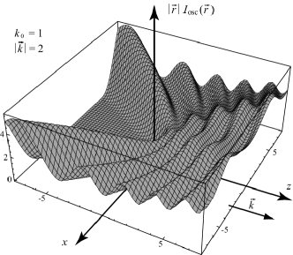
Figure 1: General field pattern of a point charge resting at the origin. The function $|\vec{r}\hskip 1.0pt|I_{\rm osc}(\vec{r}\hskip 1.0pt)$ is shown for $\vec{r}$ in the $xz$ plane with $\vec{k}$ along the $z$ direction. This function was evaluated by an analytical $|\vec{p}\hskip 1.0pt|$-type integration followed by numerical angular integrations. Uninteresting nonoscillatory pieces $I_{\rm non}$ have been subtracted for clarity, so that only the oscillatory part $I_{\rm osc}\equiv I-I_{\rm non}$ contributes to this plot. The wave pattern is resemblant to that caused by a boat moving in water.

We finally remark that single-photon emission from a massive charged particle with conventional dispersion relation $p^{2}=m^{2}$ requires spacelike photon 4-momenta: the initial and final 4-momenta of the charge each determine a point on the mass-shell hyperboloid, and the photon momentum must connect these two points. The geometry of the hyperboloid is such that any tangent, and therefore any two points, determine a spacelike direction. Note that this is also consistent with the above loop-momentum considerations.

IV Radiation rate

The rate of vacuum Čerenkov radiation can in principle be determined with the usual philosophy: extraction of the $r^{-2}$ piece of the modified Poynting vector and integration over a spherical surface. However, the integral (11) seems to evade a systematic analytical study (except in special cases), so that the determination of the asymptotic fields is challenging. We have therefore employed a method for finding the total rate of radiation that does not require explicitly the far fields.

Integration of Eq. (5) over an arbitrary volume $V$ and the divergence theorem imply

$$\int\limits_{\sigma}d\sigma^{l}\,\Theta_{l\nu}=\int\limits_{V}d^{3}\vec{r}\;j^{\mu}F_{\mu\nu}-{{\partial}\over{\partial t}}\int\limits_{V}d^{3}\vec{r}\;\Theta_{0\nu}\;,$$ (12)

where $\sigma$ is the boundary of $V$, and $d\sigma^{l}$ denotes the associated surface element with outward orientation. Thus, the energy–momentum flux $\dot{P}_{\nu}=\int_{\sigma}d\sigma^{l}\,\Theta_{l\nu}$ through the surface $\sigma$ originates from the 4-momentum generated by the source in the enclosed volume $V$ and the decrease of the field’s 4-momentum in $V$, as usual.

We are interested in 4-currents describing particles. In this case, we write $j^{\mu}(x)=J^{\mu}(x)$, where $J^{\mu}=(J^{0},\vec{J}\,)$ satisfies two general conditions in the particle’s rest frame. First, the physical situation should be stationary implying the time independence both of the 4-current and of the fields, which eliminates the last term in Eq. (12). Moreover, current conservation simplifies to $\vec{\nabla}\cdot\vec{J}=0$, so that the most general form of $J^{\mu}(x)$ is given by

$$J^{\mu}(\vec{r}\hskip 1.0pt)=\big{(}\rho(\vec{r}\hskip 1.0pt),\vec{\nabla}\!\times\!\vec{f}(\vec{r}\hskip 1.0pt)\big{)},$$ (13)

where $\rho(\vec{r}\hskip 1.0pt)$ is the charge density and $\vec{f}(\vec{r}\hskip 1.0pt)$ is an arbitrary vector field. For example, the choices $\rho(\vec{r}\hskip 1.0pt)=q\,\delta(\vec{r}\hskip 1.0pt)$ and $\vec{f}(\vec{r}\hskip 1.0pt)=\vec{\mu}\>\delta(\vec{r}\hskip 1.0pt)$ describe a point charge $q$ with magnetic moment $\vec{\mu}$ situated at the origin. Second, a particle is associated with the concept of confinement to a small spacetime region, so that we require $J^{\mu}(\vec{r}\hskip 1.0pt)$ to be localized within a finite volume $V_{0}$. Outside $V_{0}$, the 4-current is assumed to vanish rapidly. Then, $\vec{f}(\vec{r}\hskip 1.0pt)$ can be taken as localized also. However, other choices for $\vec{f}$ are possible because adding gradients to $\vec{f}$ leaves $J^{\mu}(\vec{r}\hskip 1.0pt)$ unaffected.

The zeroth component of Eq. (12) describes the radiated energy $P^{0}$. With our above considerations for $J^{\mu}(\vec{r}\hskip 1.0pt)$, the Maxwell equation $\vec{\nabla}\!\times\!\vec{E}=0$, and the divergence theorem, this component of Eq. (12) becomes

$$\int\limits_{\sigma}d\vec{\sigma}\cdot\vec{S}=-\int\limits_{\sigma}d\vec{\sigma}\cdot(\vec{f}\!\times\!\vec{E})\;,$$ (14)

where we have defined the modified Poynting vector $\Theta_{l0}=S_{l}=-S^{l}$. Since $\vec{f}(\vec{r}\hskip 1.0pt)$ is localized, the right-hand side of Eq. (14) vanishes for $V$ large enough, so that energy cannot escape to infinity. It follows that the net radiated energy is always zero in the rest frame of the (prescribed external) charge. This is unsurprising because time-translation invariance is maintained in the rest frame. The spatial localization of the system then implies energy conservation. The $P^{0}$ flux through any closed surface must therefore vanish. As an important consequence of this result, any nonzero 4-momentum radiated by a prescribed external charge in uniform motion is necessarily spacelike.

Next, we investigate the rate $\dot{P}_{s}=\int_{\sigma}d\sigma^{l}\Theta_{ls}$ at which 3-momentum is radiated. The spatial components of Eq. (12) can be written as

$$\>\dot{\!\!\vec{P}}=\int\limits_{V}d^{3}\vec{r}\;J^{\mu}\vec{\nabla}A_{\mu}\;.$$ (15)

Here, the necessary manipulations of the term containing $J^{\mu}$ involve the divergence theorem and ignoring the resulting surface integral, which is justified by the presumed spatial localization. We continue by employing the general solution (11) for $A^{\mu}$ and expressing $J^{\mu}$ in terms of its Fourier expansion in the variable $\vec{p}$. In the limit $V\rightarrow\infty$, the spatial integration yields momentum-space delta functions, and one obtains

$${}\;\;\dot{\!\!\vec{P}}=i\int\limits{{d^{3}\vec{p}}\over{(2\pi)^{3}}}\;{{\tilde{J}^{\mu}(-\vec{p}\hskip 1.0pt)N_{\mu\nu}(\vec{p}\hskip 1.0pt)\tilde{J}^{\nu}(\vec{p}\hskip 1.0pt)}\over{\vec{p}^{\,4}-4\vec{p}^{\,2}k^{2}-4(\vec{p}\!\hskip 0.8pt\cdot\!\vec{k}-i\varepsilon k_{0})^{2}}}\;\vec{p}\;,$$ (16)

as expected from Parseval’s identity. Inspection shows that the integrand is odd in $\vec{p}$. Under the additional condition that the integrand remains nonsingular for all $\vec{p}$, the radiation rate vanishes. This condition is determined by the denominator of the integrand in Eq. (16), which corresponds to the $\omega=0$ case of the dispersion relation (10). In a situation involving only timelike wave 4-vectors, which possess nonzero frequencies in any frame, regularity of the integrand is ensured precluding vacuum Čerenkov radiation. However, the presence of spacelike wave vectors in our model typically leads to singularities in the integrand in Eq. (16). Then, the $i\varepsilon$ prescription plays a determining role for the value of the integral (16).

A sample charge distribution yields further insight. The general case of a charged magnetic dipole is treated in Appendix C. Here, we focus on the simpler example of $\vec{J}=\vec{0}$. A position-space delta-function source for $\rho$ leads to an undesirable asymptotic behavior of the integrand in Eq. (16). This suggests to consider a spherical charge $q$ of finite size. We find the explicit form

$$\rho(r)={{q}\over{4\pi\lambda^{2}r}}\exp(-r/\sqrt{2}\lambda)\sin(r/\sqrt{2}\lambda)$$ (17)

to be mathematically tractable. The parameter $\lambda$ determines the size of the charge. For a quantum-mechanical particle of mass $m$, $\lambda$ might be associated with its Compton wavelength $\lambda\sim m^{-1}$. A point particle with delta-function charge distribution can be recovered in the limit $\lambda\rightarrow 0$. The Fourier transform of $\rho(r)$ is given by $\tilde{\rho}(\vec{p}\hskip 1.0pt)=q/(\vec{p}^{\,4}\lambda^{4}+1)$.

We perform the integral (16) in spherical-type coordinates with $\vec{p}=l\;(\sin\theta\cos\phi,\sin\theta\sin\phi,\cos\theta)$. It is convenient to choose the polar axis along $\vec{k}$ and to select the integration domain $l\in[-\infty,\infty]$, $\theta\in[0,\pi/2]$, and $\phi\in[0,2\pi]$. The $\phi$ integration is trivial. The $l$ integral can be evaluated with the residue theorem. Closing the contour above or below yields the same result. Note that the two dispersion-relation poles are shifted in the same imaginary direction: depending on the sign of $k_{0}$, both poles are either below or above the real-$l$ axis. The final integration over $\theta$ yields the following result:

$$\>\dot{\!\!\vec{P}}=-{{{\rm sgn}(k_{0})}\over{16\pi}}\;{{q^{2}}\over{\lambda^{2}}}\,{\rm tan}^{-1}(4k_{0}^{2}\lambda^{2})\;{{k_{0}^{2}}\over{\vec{k}^{\,2}}}\;\vec{e}_{k}\;,$$ (18)

where $\vec{e}_{k}$ denotes the unit vector in $\vec{k}$ direction. One can now take the limit $\lambda\rightarrow 0$ to obtain the radiation rate for a point charge:

$$\>\dot{\!\!\vec{P}}=-{\rm sgn}(k_{0})\;{{q^{2}}\over{4\pi}}\;{{k_{0}^{4}}\over{\vec{k}^{\,2}}}\;\vec{e}_{k}\;.$$ (19)

Note that nonzero rates are possible despite the antisymmetric integrand in Eq. (16). From a mathematical viewpoint, this essentially arises because the physical regularization prescription (i.e., the contour) fails to respect this antisymmetry. The presence of a nonzero flux in the above static case may seem counter-intuitive. However, similar situations in conventional physics can readily be identified. For example, a time-independent situation with constant non-parallel $\vec{E}$ and $\vec{B}$ fields is associated with the nonvanishing Poynting flux $\vec{S}=\vec{E}\!\times\!\vec{B}$.

In the present context, the absence of the vacuum Čerenkov effect requires $k_{0}=0$ in the rest frame. It follows in particular that for lightlike $k^{\mu}$, a point charge never ceases to emit radiation. This is to be contrasted with the conventional case, which typically involves refractive indices that imply a minimal speed of the charge for the emission of radiation. The point is that vacuum Čerenkov radiation need not necessarily be a threshold effect.

For many applications, it is more convenient to express the radiation rate (19) in the laboratory frame. Although the required coordinate change is straightforward, the resulting expressions are not particularly transparent in the general situation. We therefore focus on the spacelike-$k^{\mu}$ case and consider an inertial frame in which $k_{0}^{\prime}=0$ and $\vec{k}^{\prime}\neq\vec{0}$ (such a frame always exists). In what follows, we can suppress the primes for brevity because a confusion with the rest-frame components is excluded. For finite $\lambda$, we obtain

$$\dot{P}^{\mu}={{q^{2}}\over{16\pi}}\;{{\gamma(\vec{\beta}\!\hskip 0.8pt\cdot\!\vec{k})^{2}\lambda^{-2}}\over{\vec{k}^{\,2}+\gamma^{2}(\vec{\beta}\!\hskip 0.8pt\cdot\!\vec{k})^{2}}}\;{\rm tan}^{-1}\!\big{[}4\lambda^{2}\gamma^{2}(\vec{\beta}\!\hskip 0.8pt\cdot\!\vec{k})^{2}\big{]}\!K^{\mu},$$ (20)

and the point-charge limit gives

$$\dot{P}^{\mu}={{q^{2}}\over{4\pi}}\;{{\gamma^{3}(\vec{\beta}\!\hskip 0.8pt\cdot\!\vec{k})^{4}}\over{\vec{k}^{\,2}+\gamma^{2}(\vec{\beta}\!\hskip 0.8pt\cdot\!\vec{k})^{2}}}\;K^{\mu}.$$ (21)

Here, $\vec{\beta}$ is the 3-velocity of the charge in the laboratory and $\gamma$ is the corresponding relativistic gamma factor. The overdot now denotes laboratory-time differentiation. The 4-direction

$$K^{\mu}\equiv{{{\rm sgn}(\vec{\beta}\!\hskip 0.8pt\cdot\!\vec{k})}\over{\sqrt{\vec{k}^{\,2}+\gamma^{2}(\vec{\beta}\!\hskip 0.8pt\cdot\!\vec{k})^{2}}}}\;{\gamma^{2}(\vec{\beta}\!\hskip 0.8pt\cdot\!\vec{k})\choose\;\vec{k}+\gamma^{2}(\vec{\beta}\!\hskip 0.8pt\cdot\!\vec{k})\vec{\beta}\;}$$ (22)

arises from transforming ${\rm sgn}(k_{0})\vec{e}_{k}$. Vacuum Čerenkov radiation is absent for particle 3-velocities perpendicular to $\vec{k}$. In all other cases, both the radiated energy and the projection of the radiated 3-momentum onto the velocity are positive, which decelerates conventional charges in the chosen laboratory frame.

To determine the polarization of vacuum Čerenkov radiation, we refer to the discussion of the plane-wave solutions in Appendix B. In the particle’s rest frame, where the frequency of the emitted waves vanishes, Eq. (56) implies that the radiated electric field is purely longitudinal. In particular, plane waves emitted along $\vec{k}$ are free of $\vec{E}$ fields, i.e., they are purely magnetic. Note that the energy–momentum tensor (4) in this case remains nonzero, so that such waves are also associated with a nontrivial momentum flux.

In our laboratory frame, where $k^{0}=0$, the emitted radiation is typically left or right polarized, which can be established as follows. Consider an emitted wave with a wave vector $\vec{p}$ and select coordinates as in Appendix B. Equation (56) then yields

$$E_{y}={{p^{\mu}p_{\mu}|\vec{p}\hskip 1.0pt|}\over{2(\vec{k}\!\hskip 0.8pt\hskip 0.8pt\cdot\!\vec{p}\hskip 1.0pt)(\vec{\beta}\!\cdot\!\vec{p}\hskip 1.0pt)}}iE_{x},$$ (23)

where we have used our result from the previous section that the 4-vector of a radiated wave is of the form $p^{\mu}=(\vec{\beta}\!\hskip 0.5pt\cdot\!\vec{p},\vec{p}\hskip 1.0pt)$. The direction dependence of the polarization implied by Eq. (23) is depicted in Fig. 2. We remark that conventional Čerenkov radiation in isotropic media is linearly polarized in the plane spanned by $\vec{\beta}$ and $\vec{p}$ ll .

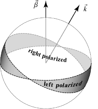
Figure 2: Dependence of the polarization on direction. For vectors $\vec{p}$ pointing in the clear (shaded) direction, the associated waves are right (left) polarized. The radiation exhibits linear polarization only when $\vec{p}$ lies on one of the dashed lines. Vacuum Čerenkov radiation may not be emitted into all directions. The wave 4-vector $p^{\mu}=(\vec{\beta}\!\cdot\!\vec{p},\vec{p}\hskip 1.0pt)$ is further constrained by the dispersion relation (10).

The conventional nondispersive Čerenkov case is associated with a conical shock wave of opening angle $\alpha=\cos^{-1}(c_{ph}/|\vec{\beta}|)$. The present model, however, is analogous to a dispersive situation, where no shock-wave singularity is expected cerclass ; certheo . This is supported by the plot in Fig. 1. The concept of a sharply defined Čerenkov cone is therefore less useful in the present context.

The more interesting question regarding the magnitude of the wave 3-vector in a given radiation direction can be answered as follows. In general, the wave vector must satisfy both the dispersion relation and the Čerenkov condition. In the laboratory frame, for example, the wave 4-vector needs to be of the form $(\vec{p}\!\hskip 0.8pt\cdot\!\vec{\beta},\vec{p}\hskip 1.0pt)$ according to the discussion in the previous section. This yields the constraint equation

$$(\vec{p}\!\hskip 0.8pt\cdot\!\vec{\beta}\hskip 1.0pt)^{2}=\vec{p}^{\,2}+2\vec{k}^{\,2}-2\sqrt{(\vec{p}\!\hskip 0.8pt\cdot\!\vec{k})^{2}+\vec{k}^{\,4}}$$ (24)

for a wave 3-vector $\vec{p}$. Here, we have again chosen a spacelike $k^{\mu}$ and selected a laboratory frame with $k^{\mu}=(0,\vec{k})$. We have further employed the dispersion-relation solution (44), where the sign choice is restricted by the Čerenkov condition of spacelike $p^{\mu}$. For a fixed $|\vec{p}\hskip 1.0pt|$, Eq. (24) determines a (distorted) cone of possible emission directions. Explicitly, denoting the angle between $\vec{\beta}$ and $\vec{p}$ by $\alpha$ and the angle between $\vec{p}$ and $\vec{k}$ by $\theta$, it follows that

$${\vec{\beta}^{2}\cos^{2}\alpha-\sin^{2}\theta\over(\vec{\beta}^{2}\cos^{2}\alpha-1)^{2}}={|\vec{p}\hskip 1.0pt|^{2}\over 4|\vec{k}\hskip 1.0pt|^{2}}.$$ (25)

Note that in Eq. (25) cylindrical symmetry about the charge’s velocity $\vec{\beta}$ is generally lost, a direct consequence of rotation breaking due to a nonzero $\vec{k}$. It is interesting to consider the case in which $|\vec{p}\hskip 1.0pt|\gg|\vec{k}\hskip 1.0pt|$. Then, Eq. (25) gives

$$\gamma^{-2}+\sin^{2}\alpha\simeq{2|\vec{\beta}\!\cdot\!\vec{k}|\over|\vec{p}\hskip 1.0pt|}\equiv\Lambda^{2}\ll 1.$$ (26)

We conclude that $\gamma>\Lambda^{-1}$, which amounts to a minimum speed of the charge for a given (large) emitted wave 3-vector, consistent with the radiation condition in Sec. III. Note also that $\alpha<\Lambda$, so that such radiation has wave 3-vectors within a small cone around $\vec{\beta}$.

In a Lorentz-violating situation as well as in conventional dispersive media, the group velocity and the wave vector need not be aligned. It follows that for a fixed $|\vec{p}\hskip 1.0pt|$ the cone determined by Eq. (24) does not necessarily coincide with the cone defined by the motion of the corresponding wave packets. At a given $|\vec{p}\hskip 1.0pt|$, this would lead us to associate the group-velocity cone rather than the phase-speed cone with the actual motion of the corresponding emitted disturbance. However, such an interpretation would be misleading. The group velocity $\vec{v}_{g}(\vec{p}\hskip 1.0pt)=\vec{\nabla}_{\!\vec{p}}\,\omega$ describes the motion of a wave packet centered at $\vec{p}$ only when all momenta $\vec{p}+d\vec{p}$ in the vicinity of $\vec{p}$ contribute to the wave packet. This is not the case in the present Čerenkov situation due to the constraint (24). In the present case, the determination of the physical velocity associated with a disturbance must only involve momenta $\vec{p}$ that satisfy Eq. (24). This corresponds to the projection of $\vec{v}_{g}(\vec{p}\hskip 1.0pt)$ onto the appropriate tangent plane of the 2-dimensional $\vec{p}\,$-space surface defined by Eq. (24). This becomes particularly clear in the charge’s rest frame. Since only waves with $\omega=0$ are emitted, differentiation of $\omega$ with respect to a radiated $\vec{p}$ must yield zero. This is consistent with the time independence of the situation: any wave pattern must be stationary in the rest frame.

V Back-reaction on the charge

Until now, the radiating charge $q$ has been considered as an external prescribed source. However, in realistic situations total energy and momentum are conserved, so that the radiated 4-momentum must be supplied by the charged particle, which will then typically undergo accelerated motion. This, in turn, leads to additional power loss through the conventional mechanism described by Larmor’s formula Jackson . A more refined analysis must therefore include aspects of the particle’s dynamics. Such an analysis is the topic of the present section. We simplify the situation by neglecting acceleration effects, so that the force acting on the charge is solely determined by the back-reaction of vacuum Čerenkov radiation.

To avoid confusion with the wave vector $p^{\mu}$, we denote the charge’s 4-momentum by $Q^{\mu}=(Q^{0},\vec{Q})$. The mass and the 4-velocity of the particle are $m$ and $u^{\mu}=\gamma(1,\vec{\beta}\hskip 1.0pt)$, respectively. We now assume energy–momentum conservation for the Čerenkov system, so that

$$\dot{Q}^{\mu}=-\dot{P}^{\mu}(\vec{\beta}\hskip 1.0pt).$$ (27)

Here, $\dot{P}^{\mu}(\vec{\beta}\hskip 1.0pt)$ is given by the rate formula (21). For particles with $Q^{\mu}=mu^{\mu}$, the relation (27) yields their equation of motion in the form of a first-order differential equation for $\vec{\beta}$, as usual. However, in quantum theory, for example, the Maxwell–Chern–Simons Lagrangian may induce a Lorentz-violating dispersion relation for the charge through radiative effects. Then, momentum and velocity of the particle need not necessarily be aligned any longer ck . and more care is required. As a result of our methodology, this issue turns out to be nontrivial even in the present classical context. Suppose the particle changes its 4-momentum by $dQ^{\mu}=-\dot{P}^{\mu}dt$ through vacuum Čerenkov radiation. The method for determining $\dot{P}^{\mu}$ discussed in the previous section then simultaneously fixes both the change in the charge’s energy and the corresponding change in its 3-momentum. We must therefore investigate the compatibility of our approach with the charge’s dispersion relation.

To answer this question, we start with the general momentum–velocity ansatz $Q^{\mu}=mu^{\mu}+q^{\mu}$, where $q^{\mu}$ is a Lorentz-violating correction that can depend on $u^{\mu}$. Time differentiation, subsequent contraction with $u_{\mu}$, and Eq. (27) yield $m\dot{u}^{\mu}u_{\mu}+\dot{P}^{\mu}u_{\mu}+\dot{q}^{\mu}u_{\mu}=0$. Differentiation of $u^{\mu}u_{\mu}=1$ with respect to time establishes that $\dot{u}^{\mu}u_{\mu}$ is always zero. In the particle’s rest frame, where the timelike component of $\dot{P}^{\mu}$ and the spacelike components of $u_{\mu}$ vanish, one verifies that $\dot{P}^{\mu}u_{\mu}=0$. We are thus left with $\dot{q}^{\mu}u_{\mu}=0$ as a constraint for our approach. Note that this condition is compatible with the conventional situation $q^{\mu}=0$, so that we are allowed to use $Q^{\mu}=mu^{\mu}$. We remark that the weakness of this constraint hinges upon our previous assumption (13) of a time-independent current distribution in the charge’s rest frame. For example, a rotating-dipole model of the charge would lead to energy emission in the center-of-mass frame, so that in general $\dot{P}^{\mu}u_{\mu}\neq 0$ requiring a dispersion-relation modification.

We can now proceed using $Q^{\mu}=mu^{\mu}$. As mentioned above, this yields the differential equation

$$-\dot{P}^{\mu}(\vec{\beta}\hskip 1.0pt)=m\dot{u}^{\mu}(\vec{\beta}\hskip 1.0pt)$$ (28)

for $\vec{\beta}(t)$, where $\dot{P}^{\mu}(\vec{\beta}\hskip 1.0pt)$ is given by the rate formula (21). It turns out that this equation can be integrated analytically in the laboratory frame with $k^{\mu}=(0,\vec{k})$. The 4-force $-\dot{P}^{\mu}(\vec{\beta}\hskip 1.0pt)$ on the charge vanishes in the spacelike direction(s) orthogonal to $\vec{\beta}$ and $\vec{k}$, so that the particle’s motion remains confined to the subspace spanned by $\vec{\beta}$ and $\vec{k}$. The relativistic Newton law (28) contains therefore at most three nontrivial equations:

$$-{{q^{2}}\over{4\pi}}\;\vec{k}^{\,2}{{\gamma^{5}\beta_{\|}^{5}}\over{(1+\gamma^{2}\beta_{\|}^{2})^{3/2}}} = m{{d}\over{dt}}\gamma,$$

$$-{{q^{2}}\over{4\pi}}\;\vec{k}^{\,2}{{\gamma^{5}\beta_{\|}^{5}}\over{(1+\gamma^{2}\beta_{\|}^{2})^{3/2}}}\,\beta_{\bot} = m{{d}\over{dt}}\gamma\beta_{\bot},$$

$$-{{q^{2}}\over{4\pi}}\;\vec{k}^{\,2}{{\gamma^{3}\beta_{\|}^{3}}\over{(1+\gamma^{2}\beta_{\|}^{2})^{1/2}}}\,\beta_{\|} = m{{d}\over{dt}}\gamma\beta_{\|}.$$ (29)

Here, $\beta_{\|}$ and $\beta_{\bot}$ denote the respective magnitudes of the $\vec{\beta}$-velocity components parallel and perpendicular to $\vec{k}$, so that $\gamma^{-2}=1-\beta_{\|}^{2}-\beta_{\bot}^{2}$.

Note that the three equations of motion (29) determine two unknown functions, the velocity components $\beta_{\bot}(t)$ and $\beta_{\|}(t)$. Compatibility with the dispersion-relation constraint discussed above guarantees that only two of these equations are independent, as required by consistency. To see this explicitly, note that the first and the second of the equations of motion (29) imply

$$\beta_{\bot}(t)=\beta_{\bot}=\text{const.}$$ (30)

Introducing the variable $\xi\equiv\gamma\beta_{\|}$ one can now demonstrate that all three components of the equations of motion (29) lead to the same differential equation for $\xi$, and thus $\beta_{\|}$, given by

$$-{{q^{2}}\over{4\pi}}\;\vec{k}^{\,2}\sqrt{1-\beta_{\bot}^{2}}{{\xi^{4}}\over{1+\xi^{2}}}=m{{d}\over{dt}}\xi.$$ (31)

This result establishes the dependency among the equations, and it is suitable for integration. We obtain

$${{1}\over{\xi}}+{{1}\over{3\xi^{3}}}={{t+t_{0}}\over{\tau}},$$ (32)

where $\tau=4\pi m/q^{2}\vec{k}^{\,2}\sqrt{1-\beta_{\bot}^{2}}$ is the characteristic time scale associated with the particle’s motion. The integration constant $t_{0}\geq 0$ is determined by the velocity of the particle at $t=0$. Note that as the time increases, the parameter $\xi$, and thus $\beta_{\|}$, decrease, so that the charge is always slowed down by vacuum Čerenkov radiation when viewed in our laboratory frame.

Although Eq. (32) can be solved analytically for $\beta_{\|}(t)$, the resulting expression is not particularly transparent. We therefore consider certain limiting cases. Suppose $\xi\gg 1$, which corresponds to a fast-moving charge. Then, the $\xi^{-3}$ term in Eq. (32) can be neglected and one obtains

$$\beta_{\|}(t)={{4\pi m}\over{q^{2}\vec{k}^{\,2}}}\;{{1}\over{\sqrt{(t+t_{0})^{2}+\tau^{2}}}}.$$ (33)

The corresponding distance $d_{\|}$ traveled parallel to $\vec{k}$ is given by

$$d_{\|}(t)={{4\pi m}\over{q^{2}\vec{k}^{\,2}}}\left(\sinh^{-1}{{t+t_{0}}\over{\tau}}-\sinh^{-1}{{t_{0}}\over{\tau}}\right).$$ (34)

Since $d_{\bot}=\beta_{\bot}t$, the trajectory is in general no longer a straight line. The path of a fast charge is determined by a hyperbolic-sine function with a characteristic scale size of $\beta_{\bot}\tau$. Such a curved trajectory is a direct consequence of the involved vacuum anisotropies.

In the case of a charge moving with a nonrelativistic $\beta_{\|}$ satisfying $\beta_{\|}^{2}\ll 1-\vec{\beta}^{\,2}$, we have $\xi\ll 1$. It follows that the $\xi^{-1}$ term in Eq. (32) is negligible, so that

$$\beta_{\|}(t)={{\tau^{1/3}\sqrt{1-\beta_{\bot}^{2}}}\over{\sqrt{3^{2/3}(t+t_{0})^{2/3}+\tau^{2/3}}}}.$$ (35)

This expression can be integrated analytically to yield

$$d_{\|}(t)={{2\pi m}\over{q^{2}\vec{k}^{\,2}}}\left[h\left(3{{t+t_{0}}\over{\tau}}\right)-h\left(3{{t_{0}}\over{\tau}}\right)\right]$$ (36)

for the distance $d_{\|}$ traveled parallel to $\vec{k}$. Here, the function $h$ is given by

$$h(\chi)\equiv\chi^{1/3}\sqrt{1+\chi^{2/3}}+\sinh^{-1}(\chi^{1/3}).$$ (37)

For large $t\gg\tau$, the parallel distance traveled increases as $t^{2/3}$, so that not even asymptotically a straight-line trajectory arises. If one extrapolates these results to the curved-spacetime situation, it follows that in the Einstein–Maxwell–Chern–Simons system grav a conventional test charge would not travel along traditional geodesics despite the absence of external electromagnetic fields. Such a violation of the equivalence principle is seen to be closely tied to the presence of Lorentz breaking.

VI Phase-space estimate

A quantum-field treatment of vacuum Čerenkov radiation would be desirable. However, such an analysis requires a completely satisfactory quantum theory of the model under consideration, a condition that is not met in most Lorentz-violating frameworks. In fact, many approaches to Lorentz breaking lack a Lagrangian and are purely kinematical precluding even a classical analysis along the lines presented above. Although such models are theoretically less attractive, it is still interesting to investigate to which degree a modified dispersion relation by itself can give insight into vacuum Čerenkov radiation.

In quantum field theory, the rate $\Gamma$ for the decay of a particle $P_{a}$ into two particles, $P_{b}$ and $P_{c}$, obeys

$$d\Gamma={{|{\cal M}_{a\rightarrow b,c}|^{2}}\over{2E_{a}}}(2\pi)^{4}\delta^{(4)}(p_{a}^{\mu}-p_{b}^{\mu}-p_{c}^{\mu})d\Pi_{b}d\Pi_{c}.$$ (38)

Here, ${\cal M}_{a\rightarrow b,c}$ is the transition amplitude containing information about the dynamics of the decay. The remaining quantities are associated with the kinematics of the reaction process. They include phase-space elements $d\Pi_{s}$ and various 4-momenta $p_{s}^{\mu}=(E_{s},\vec{p}_{s})$, where the subscript $s\in\{a,b,c\}$ refers to the corresponding particle. In what follows, we take $P_{a}$ and $P_{b}$ to be a charge $q$ with conventional dispersion relation $p_{a}^{2}=p_{b}^{2}=m^{2}$. For comparison with the classical result (19), we consider photons $P_{c}$ with a dispersion relation corresponding to that of classical plane waves in the Maxwell–Chern–Simons model for lightlike $k^{\mu}$ (43). In particular, we identify the wave frequency $\omega$ with the photon energy $E_{c}$.

To leading approximation, the determination of ${\cal M}_{a\rightarrow b,c}$ is expected to parallel that of the conventional case: contraction of the photon polarization 4-vector with a $q\gamma^{\mu}$-type vertex sandwiched between two external-leg spinors. It follows that the amplitude ${\cal M}_{a\rightarrow b,c}$ transforms as a coordinate scalar fn3 . As an important consequence, the rest-frame and the laboratory-frame amplitudes of a given decay cannot differ by relativistic $\gamma$ factors, which could mask the true energy dependence of the reaction rate. Note, however, that this does not imply particle Lorentz symmetry in ${\cal M}_{a\rightarrow b,c}$. Note also that ${\cal M}_{a\rightarrow b,c}$ is typically energy dependent: with our normalization, the spinor components scale as the square root of their energy, and the components of photon polarization vectors are of order unity. With these considerations, we can take ${\cal M}_{a\rightarrow b,c}=qE_{a}M$ as the generic form of the amplitude kauf . The dimensionless function $M$ is determined by the model’s dynamics and depends on external momenta and the Lorentz-violating parameters.

The decay rate $\Gamma$, defined as the coordinate-scalar transition probability per time, must pick up a time-dilation factor under coordinate boosts. On the right-hand side of Eq. (38), the $E_{a}^{-1}$ normalization provides this transformation property, so that the remaining part of this expression is a scalar under observer transformations. This implies that the phase-space elements $d\Pi_{s}$ must also transform as coordinate scalars (see previous footnote fn3 ). For Lorentz-symmetric dispersion relations and in our normalization, $d\Pi$ is determined by the conventional relation $2E_{\vec{p}}\,(2\pi)^{3}d\Pi=d^{3}\vec{p}$, where $E_{\vec{p}}$ is a dispersion-relation root at $\vec{p}$. This applies only to the charge in the present example, so that $d\Pi_{b}$ in Eq. (38) is conventional. However, for Lorentz-violating dispersion relations, such as that of our photon, this expression is no longer coordinate independent. It can be verified that for the positive-energy, spacelike branches of the present modified photon dispersion relation (43) the phase-space element

$$d\Pi_{c}={{d^{3}\vec{p}_{c}}\over{(2\pi)^{3}2|\vec{p}_{c}+{\rm sgn}(k^{0})\vec{k}|}}$$ (39)

is observer invariant. As discussed previously, the kinematics of the Čerenkov process requires spacelike photon 4-momenta, so that Eq. (39) is indeed the relevant one in the present context. Note that for zero $k^{\mu}$ the conventional expression is recovered.

With our above considerations Eq. (38) becomes

$$d\Gamma={{q^{2}|M|^{2}m}\over{32\pi^{2}}}\;{{\delta^{(4)}(p_{a}^{\mu}-p_{b}^{\mu}-p_{c}^{\mu})\>d^{3}\vec{p}_{b}\>d^{3}\vec{p}_{c}}\over{\sqrt{\vec{p}_{b}^{\,2}+m^{2}}\;|\vec{p}_{c}+{\rm sgn}(k^{0})\vec{k}|}}$$ (40)

in the charge’s rest frame. The $\vec{p}_{b}$ integration can be performed straightforwardly. For the $\vec{p}_{c}$ integral we select spherical coordinates with $\vec{k}$ along the polar axis. We denote the azimuthal and polar angles by $\theta$ and $\phi$, respectively. The limit of a nondynamical charge, which is necessary for comparison with the previous classical treatment, can be recovered here for $m\to\infty$. Then, the remaining delta function gives the constraint $|\vec{p}_{c}|=-2\>k^{0}\cos\theta$. We remark that this condition implies zero-energy photons as decay products consistent with our previous dynamical analysis in the classical context. Note also that this constraint restricts the angular integrations to the upper or lower hemisphere depending on the sign of $k^{0}$. The $|\vec{p}_{c}|$ integration now yields

$${{d\Gamma}\over{d\Omega}}=-{{q^{2}|M|^{2}}\over{8\pi^{2}}}k^{0}\cos\theta$$ (41)

for the differential decay rate in the charge’s rest frame. Here, $\Omega$ denotes the solid angle.

For the remaining angular integrations, the functional dependence $M=M(\Omega)$ is needed. However, we are interested in a rough approximation for the decay rate only, so that it appears reasonable to replace $|M(\Omega)|^{2}$ by a constant $\overline{|M|^{2}}\sim{\cal O}(1)$ corresponding perhaps to a suitable angular average of $|M(\Omega)|^{2}$. Then, an estimate for the total decay rate is given by $\Gamma\simeq(8\pi)^{-1}\overline{|M|^{2}}q^{2}|\vec{k}|$. Noting that $d\dot{P}^{\mu}=p^{\mu}(\Omega)\,d\Gamma$, the rate of momentum emission can be determined similarly. We obtain

$$\>\dot{\!\!\vec{P}}\simeq-{\rm sgn}(k^{0}){{q^{2}\overline{|M|^{2}}}\over{8\pi}}\vec{k}^{\,2}\vec{e}_{k}$$ (42)

as an estimate for the net radiated momentum per time in the charge’s rest frame. Comparison with Eq. (19) obtained from the corresponding classical treatment reveals agreement (up to the indeterminate numerical factor $\overline{|M|^{2}}$) with the above phase-space estimate (42).

This result demonstrates that a careful kinematical analysis of the Čerenkov decay can give a sensible estimate for the rate of momentum emission. Note, however, the assumptions involved: equality of plane-wave and one-particle dispersion relations, absence of additional symmetries suppressing the quantum amplitude, and a nondynamical Lorentz-symmetric charge $m\rightarrow\infty$. We also emphasize the importance of constructing invariant phase-space elements in the present context.

VII Experimental outlook

This section mentions some examples of potentially observable signatures for Lorentz violation in the context of vacuum Čerenkov radiation. Such experimental effects can be grouped into two broad classes: detection of the emitted radiation itself through its properties analyzed in Sec. IV and effects on the charge’s motion discussed in Sec. V.

Searches for the emitted electromagnetic radiation are perhaps suggested by the analogous discovery of the conventional Čerenkov effect. In the present case, a fast charged particle should radiate left or right polarized waves into directions determined by Eq. (24). The phase-speed condition and the dispersion relation (10) imply that the maximum frequency emitted obeys $\omega_{\textrm{max}}\mathrel{\hbox to0.0pt{\lower 3.0pt\hbox{$\sim$}\hss}\raise 2.0pt\hbox{$<$}}\gamma^{2}\>{\cal O}(k^{\mu})$. Here, $\gamma$ is the boost factor corresponding to the charge’s speed and ${\cal O}(k^{\mu})$ denotes the typical size of $k^{\mu}$ components in the laboratory frame, which are observationally constrained by ${\cal O}(k^{\mu})\mathrel{\hbox to0.0pt{\lower 3.0pt\hbox{$\sim$}\hss}\raise 2.0pt\hbox{$<$}}10^{-42}\,$GeV mcsclass . Taking this bound to be saturated, we find for the example a proton at the end of the observed cosmic-ray spectrum ($10^{20}\,$eV) that $\omega_{\textrm{max}}$ is of the order of $1.6\times 10^{4}\,$rad/s corresponding to a wavelength of $1.2\times 10^{5}\,$m. On a speculative note, such radiation might perhaps be observable in high-energy astrophysical jets emitted in the direction of sight.

The presence of Lorentz violation in electrodynamics can also affect the motion of particles via the vacuum Čerenkov effect. For example, a high-energy charge would be slowed down due to the emission of radiation. This would lead to an effective cut-off in the cosmic-ray spectrum for primary particles carrying an electric charge or a magnetic dipole moment. This idea has been widely employed in the literature to place bounds on Lorentz breaking. In the present Maxwell–Chern–Simons model, which is already tightly constrained by other considerations, the energy-loss rate is suppressed by two powers of the Lorentz-violating coefficient $k^{\mu}$. However, it would be interesting to consider the dimensionless $k_{F}$ term in the SME: some of its components are currently only bounded at the $10^{-9}$ level cavexpt , and a dynamical study paralleling the present one could yield less suppressed rates.

Another potential signature associated with the charge’s motion is of statistical nature. Consider, for instance, Eq. (21), which is valid in a laboratory frame with purely spacelike $k^{\mu}=(0,\vec{k})$. In this frame, particles with velocities $\vec{\beta}$ that are perpendicular to $\vec{k}$ cease to radiate. Thus, the presence of a spacelike $k^{\mu}$ during most of the cosmological history would constrain the average motion of charges to 3-velocities lying in a two-dimensional plane. This effect might be more efficient before electroweak symmetry breaking for two reasons. First, radiation is not yet decoupled from the matter, so that there are a large number of free charges that can be affected. Second, massless charged matter is associated with lightlike 4-momenta so that all wave frequencies can contribute to vacuum Čerenkov radiation. Investigations in such a context might therefore provide stringent complementary Lorentz-violation bounds.

VIII Conclusions

Lorentz-violating vacua can arise in various approaches to fundamental physics and are described at low energies by the SME. In this paper, we have considered the physics of electrodynamics in such vacua, which exhibits close parallels to the conventional Maxwell case in macroscopic media. Our study has focused on vacuum Čerenkov radiation, which is the analogue of the usual Čerenkov effect whereby light is emitted from charges moving uniformly with superluminal speeds in a medium. Although we have performed our analysis primarily within the classical Maxwell–Chern–Simons limit of the SME, we expect most results and our methodology to remain applicable in more general cases including non-electromagnetic ones.

In Sec. III, we have developed a qualitative physical picture of the Čerenkov effect for general situations that augments the usual one in macroscopic media. It also permits an alternative extraction the general radiation condition: energy–momentum transport to infinity, and thus radiation, can only occur when the fields fall of like $r^{-1}$. This in turn requires that purely spacelike wave 4-vectors satisfy the electromagnetic plane-wave dispersion relation in the charge’s rest frame.

Based on this intuitive physical picture, we have developed a method complementing the conventional one for the determination of the 4-momentum flux associated with Čerenkov radiation. The advantage of this procedure lies in the fact that it does not require the explicit knowledge of the far fields. In the Maxwell–Chern–Simons model, our method permits the calculation of the exact 4-momentum radiation rate for a prescribed point charge with magnetic moment. The corresponding polarization of the emitted vacuum Čerenkov radiation follows from Eq. (23) and is depicted in Fig. 2.

Section V has treated the effects of vacuum Čerenkov radiation on the charge. Within our framework, the back-reaction provides a nontrivial constraint on the dispersion relation of the charge. For reasonable models of the charge’s 4-current distribution, this constraint is mild enough to allow the conventional Lorentz-symmetric 3-momentum dependence of the energy. As part of our discussion, we have determined the modified trajectory of a point charge in the Maxwell–Chern–Simons model, which remains no longer a geodesic. This type of equivalence-principle violation appears generic in the presence of vacuum Čerenkov radiation.

In some situations, useful insight into the Čerenkov-radiation rate can be obtained by purely kinematical considerations. We have exemplified this in Sec. VI by a detailed phase-space estimate that involves photons obeying the Maxwell–Chern–Simons plane-wave dispersion relation. We found that the construction of coordinate-independent phase-space elements in the presence of Lorentz breaking is an important nontrivial issue. when Lorentz symmetry is violated.

Appendix A Dispersion relation

For a given wave 3-vector $\vec{p}$, the dispersion relation (10) determines the corresponding values for $\omega$. In the lightlike-$k^{\mu}$ case, one obtains

$$\omega^{(n)}_{\pm}=\pm|\vec{p}+(-1)^{n}\vec{k}|-(-1)^{n}k^{0},$$ (43)

where $n\in\{1,2\}$. For purely spacelike $k^{\mu}=(0,\vec{k})$, the plane-wave frequencies are given by

$$\omega^{(n)}_{\pm}=\pm\sqrt{\vec{p}^{\,2}+2\vec{k}^{\,2}+2(-1)^{n}\sqrt{\vec{k}^{\,4}+(\vec{p}\!\hskip 0.8pt\cdot\!\vec{k})^{2}}}.$$ (44)

If $k^{\mu}=(k^{0},\vec{0})$ is purely timelike, the solutions of the dispersion relation are

$$\omega^{(n)}_{\pm}=\pm\sqrt{\vec{p}^{\,2}+2(-1)^{n}k^{0}|\vec{p}\hskip 1.0pt|}.$$ (45)

Note that branches determining spacelike wave 4-vectors occur in each of the canonical cases (43), (44), and (45).

For general $k^{\mu}$, the exact roots of the dispersion relation (10) can also be obtained straightforwardly. However, they are less transparent, so that we only give expressions that are correct to first order in the Lorentz-violating parameter $k^{\mu}$. Without loss of generality we can rotate the coordinate system such that $p^{\mu}=(\omega,0,0,p_{z})$ and $k^{\mu}=(k^{0},|\vec{k}|\sin\theta,0,|\vec{k}|\cos\theta)$. The approximate solutions are then given by

$$\omega^{(n)}_{\pm}=\pm p_{z}+(-1)^{n}(k^{0}\mp|\vec{k}|\cos\theta).$$ (46)

We note that we have selected convenient labels for these first-order results, which do not necessarily correspond to the labels for the canonical cases discussed earlier.

In Fig. 3, the plane-wave frequencies $\omega^{(n)}_{\pm}$ are plotted versus $p_{z}$ in some appropriate units for $k^{0}=1$, $|\vec{k}|=2$, and $\theta=1/2$. The solid lines represent the four branches of the exact roots and the broken ones the corresponding first-order solutions (46). The interior of the $p^{\mu}$-space lightcone has been shaded. For a given nonzero wave 3-vector, there are two timelike and two spacelike wave 4-vectors satisfying the dispersion relation, as expected from the above discussion of the three canonical cases.

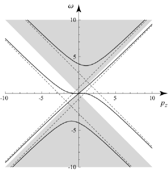
Figure 3: Sample solution of the plane-wave dispersion relation. The solid lines correspond to the exact roots. The first-order solutions are shown as broken lines. The shaded region represents the interior of the $p^{\mu}$-space lightcone.

Appendix B Plane-wave solutions

A plane-wave ansatz $A^{\nu}(x)=A_{p}^{\nu}(p)\exp(-ip\!\hskip 0.8pt\cdot\!x)$ in Eq. (2) for $j^{\mu}=0$ gives

$$\left(p_{\mu}p_{\nu}-p^{2}\eta_{\mu\nu}+2i\varepsilon_{\mu\nu\rho\sigma}k^{\rho}p^{\sigma}\right)A_{p}^{\nu}(p)=0.$$ (47)

In what follows, we adopt Lorentz gauge $p\!\cdot\!A=0$ and the following coordinates: $\vec{p}=p_{z}\vec{e}_{z}$ and $\vec{k}=k_{x}\vec{e}_{x}+k_{z}\vec{e}_{z}$, where $\vec{e}_{x}$ and $\vec{e}_{z}$ are the usual unit vectors in the 1- and 3-direction, respectively. For $p^{\mu}$ satisfying the plane-wave dispersion relation (10), the polarization vectors

$$A_{p}^{\nu}(\omega,\vec{p}\hskip 1.0pt)={{g}\over{2p_{z}}}\left(\begin{array}[]{c}2k_{x}p_{z}\\ 2(k_{0}p_{z}-k_{z}\omega)\\ -i(\omega^{2}-p_{z}^{2})\\ 2k_{x}\omega\end{array}\right)$$ (48)

obey Eq. (47), where $g$ is a constant.

The electric field $\vec{E}(x)=\vec{E}_{p}(\omega,\vec{p}\hskip 1.0pt)\exp(-ip\!\hskip 0.8pt\cdot\!x)$ and the magnetic field $\vec{B}(x)=\vec{B}_{p}(\omega,\vec{p}\hskip 1.0pt)\exp(-ip\!\hskip 0.8pt\cdot\!x)$ of the plane wave are now determined by the conventional field–potential relationship, so that the polarization vectors are

$$\vec{E}_{p}(\omega,\vec{p}\hskip 1.0pt) = {{ig}\over{2p_{z}}}\left(\begin{array}[]{c}2\omega(k_{0}p_{z}-k_{z}\omega)\\ -i\omega(\omega^{2}-p_{z}^{2})\\ 2k_{x}(\omega^{2}-p_{z}^{2})\end{array}\right),$$ (52)

$$\vec{B}_{p}(\omega,\vec{p}\hskip 1.0pt) = {{ig}\over{2}}\left(\begin{array}[]{c}i(\omega^{2}-p_{z}^{2})\\ 2(k_{0}p_{z}-k_{z}\omega)\\ 0\end{array}\right).$$ (56)

The physical fields are understood to be given by the real parts of the resulting plane-wave expressions, as usual. The magnetic field remains transverse because the homogeneous equation $\vec{\nabla}\!\cdot\!\vec{B}=0$ is unaltered. Note, however, that the electric field can exhibit longitudinal components.

In conventional optics, a plane wave is called left (right) polarized, when the electric-field vector rotates (counter)clockwise around the wave vector $\vec{p}$ at a fixed point in space for an observer looking in the direction of propagation Jackson . In the present context, we adopt the analogous definition involving the motion of the transverse electric-field component $\vec{E}_{\bot}$. One can then distinguish between elliptical polarization, and the limiting cases of linear and circular polarization, as usual. An important example is the case in which the wave vector $\vec{p}$ is large compared to the components of $k^{\mu}$. Then, Eqs. (46) and (56) give $E_{y}=\mp(-1)^{n}iE_{x}$, where the upper (lower) sign corresponds to waves of positive (negative) frequency. The longitudinal component of $\vec{E}$ vanishes in this limit. It follows that such waves exhibit the conventional circular polarizations.

Note that the above definition of polarization can fail in certain circumstances. For instance, it follows from Eq. (56) that zero-frequency waves, such as Čerenkov radiation in the charge’s rest frame, are associated with $\vec{E}_{\bot}=\vec{0}$. The electric field is then purely longitudinal (or zero) precluding any of the transverse polarizations. Although it leaves unaffected the polarization, we also remark that for waves with a phase speed $c_{ph}<1$ the direction of propagation, which is involved in the polarization definition, is observer dependent.

Appendix C Charged magnetic dipoles

In this appendix, we refine our model of the charged particle by including a magnetic moment $\vec{\mu}$ into our analysis. This is phenomenologically interesting because all known electrically charged elementary particles carry nonzero spin, which is associated with a finite magnetic moment. Moreover, the $q=0$ limit of the model then describes the Čerenkov effect in the presence of neutral particles with magnetic moments, such as neutrons.

The rest-frame current distribution $J^{\mu}$ of a point magnetic dipole $\vec{\mu}$ with charge $q$ located at the origin is given by $J^{\mu}(\vec{r}\hskip 1.0pt)=\big{(}q\,\delta(\vec{r}\hskip 1.0pt),-\vec{\mu}\!\hskip 1.2pt\times\!\vec{\nabla}\delta(\vec{r}\hskip 1.0pt)\big{)}$, as mentioned previously in the discussion of ansatz (13). To force convergence in certain intermediate steps of the calculation, we write $\delta(\vec{r}\hskip 1.0pt)=\lim_{\lambda\to 0}f(r,\lambda)$ for the delta function, where

$$f(r,\lambda)={{1}\over{4\pi\lambda^{2}r}}\exp(-r/\sqrt{2}\lambda)\sin(r/\sqrt{2}\lambda)$$ (57)

paralleling the pure-charge case in Sec. IV. We remark that the magnetic-moment definition $\vec{\mu}={\textstyle{1\over 2}}\int\vec{r}\!\hskip 0.5pt\times\!\vec{J}\>d^{3}r$ in classical electrodynamics Jackson is consistent with our choice of current for all $\lambda$. The charge density, and thus its Fourier image, remain unchanged relative to those used in Sec. IV. The 3-current $\vec{J}(\vec{r}\hskip 1.0pt)$ takes the form ${}\,\tilde{\!\vec{J}}(\vec{p}\hskip 1.0pt)=i(\vec{p}\!\hskip 0.8pt\times\!\vec{\mu})(\lambda^{4}\vec{p}^{\,4}+1)^{-1}$ in Fourier space.

Next, we use Eq. (16) to obtain an explicit integral expression for the radiation rate in the dipole’s rest frame:

$$\>\dot{\!\!\vec{P}}=i\int{{d^{3}\vec{p}}\over{(2\pi)^{3}}}\;{{\vec{p}^{\,2}\big{[}q^{2}-(\vec{p}\!\hskip 0.8pt\times\!\vec{\mu})^{2}\big{]}+4q\big{[}(\vec{k}\!\hskip 0.8pt\cdot\!\vec{p}\hskip 1.0pt)(\vec{\mu}\!\hskip 0.8pt\cdot\!\vec{p}\hskip 1.0pt)-(\vec{k}\!\hskip 0.8pt\cdot\!\vec{\mu})\vec{p}^{\,2}\big{]}-4\big{[}\vec{p}\!\hskip 0.8pt\cdot\!(\vec{k}\!\hskip 0.8pt\times\!\vec{\mu})\big{]}^{2}-4q^{2}k_{0}^{2}}\over{\big{[}\vec{p}^{\,4}-4\vec{p}^{\,2}k^{2}-4(\vec{k}\!\hskip 0.5pt\cdot\!\vec{p}-i\varepsilon k_{0})^{2}\big{]}\big{[}\lambda^{4}\vec{p}^{\,4}+1\big{]}^{2}}}\;\vec{p}\;.$$ (58)

We perform this integration in spherical-type coordinates with $\vec{p}=l\;(\sin\theta\cos\phi,\sin\theta\sin\phi,\cos\theta)$. We select the polar axis along $\vec{k}$, and $\vec{\mu}$ lies in the $xz$ plane such that $\vec{\mu}=|\vec{\mu}\hskip 0.5pt|\,(\sin\alpha,0,\cos\alpha)$. To apply complex-integration methods, we chose the integration domain $l\in[-\infty,\infty]$, $\theta\in[0,\pi/2]$, and $\phi\in[0,2\pi]$, as before. The $l$ integral can then be evaluated with the residue theorem.

As discussed before, finite emission rates can arise only in the presence of poles at real $l$. Only the dispersion-relation part of the denominator in the integral (58) with zeros at $l_{\pm}=\pm 2(k_{0}^{2}-\vec{k}^{\,2}\sin^{2}\theta)^{1/2}$ can lead to such poles. The corresponding values for $\theta$ that also lie within the above range of integration are determined by $(1-k_{0}^{2}/\vec{k}^{\,2})^{1/2}\leq\cos\theta\leq 1$. In this case, the contour for the $l$ integration is fixed by the causal $i\varepsilon$ prescription: up to an unimportant normalization of $\varepsilon$, the poles are shifted to $l_{\pm}\to\,l_{\pm}-i\varepsilon\,\text{sgn}(k_{0})$. Suppose $k_{0}>0$, so that the contour passes above the real poles at $l_{\pm}$. We then choose to close the integration contour above encircling the poles at $l^{\pm}=(\pm 1+i)/\sqrt{2}\lambda$ with the respective residues $R^{\pm}(\lambda,\alpha,\theta,\phi)$. It is now straightforward to evaluate the $l$ integral with the aid of the residue theorem. We obtain

$${}\;\;\dot{\!\!\vec{P}}=-\!\!\!\!\!\!\!\!\!\!\!\int\limits_{\sqrt{1-k_{0}^{2}/\vec{k}^{\,2}}}^{1}\!\!\!\!\!\!\!\!\!\!d\cos\theta\!\int\limits_{0}^{2\pi}\!d\phi\;{{R^{+}+R^{-}}\over{(2\pi)^{2}}}\left(\begin{array}[]{c}\sin\theta\cos\phi\\ \sin\theta\sin\phi\\ \cos\theta\end{array}\right).$$ (59)

We remark that an analogous calculation in situations with $k_{0}<0$ gives the same expression with the opposite sign provided the symmetries of the residues are taken into account.

For further progress, we use the explicit form of the residues $R^{\pm}(\lambda,\alpha,\theta,\phi)$ and take the point-particle limit $\lambda\to 0$. This permits a closed-form evaluation of the remaining angular integrals:

$${}\;\dot{\!\!\vec{P}}=-{{{\rm sgn}(k_{0})}\over{12\pi}}\;{{k_{0}^{5}}\over{|\vec{k}|^{5}}}\left\{\left[3q^{2}\vec{k}^{\,2}/k_{0}^{2}+6q\,\vec{k}\!\hskip 0.8pt\cdot\!\vec{\mu}-\vec{\mu}^{\,2}k_{0}^{2}+5(\vec{k}\!\hskip 0.8pt\cdot\!\vec{\mu})^{2}k_{0}^{2}/\vec{k}^{\,2}+10(\vec{k}\!\hskip 0.8pt\times\!\vec{\mu})^{2}\right]k_{0}\vec{k}-2\left[q\vec{k}^{\,2}/k_{0}^{2}+\vec{k}\!\hskip 0.8pt\cdot\!\vec{\mu}\right]k_{0}^{3}\,\vec{\mu}\right\}.$$ (60)

Equation (60) gives the exact expression for the net momentum radiated by a charged pointlike magnetic dipole as measured in its rest frame. In the $\vec{\mu}\to\vec{0}$ limit, our previous result (19) for a point charge is recovered. The leading-order corrections to the point-charge rate (19) arising from the presence of the magnetic moment $\vec{\mu}$ are suppressed by an additional power of $k^{\mu}$, as expected on dimensional grounds. Although heavily suppressed by four powers of $k^{\mu}$, the rate does remain nonzero in the pure-dipole limit $q\to 0$.

References

- (1) For an overview see, e.g., CPT and Lorentz Symmetry II, edited by V.A. Kostelecký (World Scientific, Singapore, 2002).
- (2) D. Colladay and V.A. Kostelecký, Phys. Rev. D 55, 6760 (1997); 58, 116002 (1998).
- (3) V.A. Kostelecký, Phys. Rev. D 69, 105009 (2004).
- (4) V.A. Kostelecký and R. Lehnert, Phys. Rev. D 63, 065008 (2001).
- (5) V.A. Kostelecký and S. Samuel, Phys. Rev. D 39, 683 (1989); Phys. Rev. Lett. 66, 1811 (1991); V.A. Kostelecký and R. Potting, Nucl. Phys. B 359, 545 (1991); Phys. Lett. B 381, 89 (1996); Phys. Rev. D 63, 046007 (2001); V.A. Kostelecký, M.J. Perry, and R. Potting, Phys. Rev. Lett. 84, 4541 (2000).
- (6) R. Gambini and J. Pullin, in Ref. cpt01 ; J. Alfaro, H.A. Morales-Técotl, and L.F. Urrutia, Phys. Rev. D 66, 124006 (2002); D. Sudarsky, L. Urrutia, and H. Vucetich, Phys. Rev. Lett. 89, 231301 (2002); Phys. Rev. D 68, 024010 (2003); G. Amelino-Camelia, Mod. Phys. Lett. A 17, 899 (2002); Y.J. Ng, Mod. Phys. Lett. A18, 1073 (2003); R.C. Myers and M. Pospelov, Phys. Rev. Lett. 90, 211601 (2003); N.E. Mavromatos, Nucl. Instrum. Meth. B 214, 1 (2004).
- (7) See, however, C.N. Kozameh and M.F. Parisi, Class. Quant. Grav. 21, 2617 (2004).
- (8) C. Adam and F.R. Klinkhamer, Nucl. Phys. B 607, 247 (2001); F.R. Klinkhamer and C. Rupp, hep-th/0312032.
- (9) S.M. Carroll et al., Phys. Rev. Lett. 87, 141601 (2001); Z. Guralnik, R. Jackiw, S.Y. Pi, and A.P. Polychronakos, Phys. Lett. B 517, 450 (2001); C.E. Carlson, C.D. Carone, and R.F. Lebed, Phys. Lett. B 518, 201 (2001); A. Anisimov, T. Banks, M. Dine, and M. Graesser, Phys. Rev. D 65, 085032 (2002); I. Mocioiu, M. Pospelov, and R. Roiban, Phys. Rev. D 65, 107702 (2002); M. Chaichian, M.M. Sheikh-Jabbari, and A. Tureanu, hep-th/0212259; J.L. Hewett, F.J. Petriello, and T.G. Rizzo, Phys. Rev. D 66, 036001 (2002).
- (10) V.A. Kostelecký, R. Lehnert, and M.J. Perry, Phys. Rev. D 68, 123511 (2003); O. Bertolami, R. Lehnert, R. Potting, and A. Ribeiro, Phys. Rev. D 69, 083513 (2004).
- (11) N. Arkani-Hamed, H.-C. Cheng, M.A. Luty, and S. Mukohyama, JHEP 0405, 074 (2004).
- (12) C.D. Froggatt and H.B. Nielsen, hep-ph/0211106.
- (13) J.D. Bjorken, Phys. Rev. D 67, 043508 (2003).
- (14) C.P. Burgess et al., JHEP 0203, 043 (2002); A.R. Frey, JHEP 0304, 012 (2003); J. Cline and L. Valcárcel, JHEP 0403, 032 (2004).
- (15) KTeV Collaboration, H. Nguyen, in Ref. cpt01 ; OPAL Collaboration, R. Ackerstaff et al., Z. Phys. C 76, 401 (1997); DELPHI Collaboration, M. Feindt et al., preprint DELPHI 97-98 CONF 80 (1997); BELLE Collaboration, K. Abe et al., Phys. Rev. Lett. 86, 3228 (2001); BaBar Collaboration, B. Aubert et al., hep-ex/0303043; FOCUS Collaboration, J.M. Link et al., Phys. Lett. B 556, 7 (2003).
- (16) V.A. Kostelecký and R. Potting, Phys. Rev. D 51, 3923 (1995).
- (17) D. Colladay and V.A. Kostelecký, Phys. Lett. B 344, 259 (1995); Phys. Rev. D 52, 6224 (1995); V.A. Kostelecký and R. Van Kooten, Phys. Rev. D 54, 5585 (1996); O. Bertolami et al., Phys. Lett. B 395, 178 (1997); N. Isgur et al., Phys. Lett. B 515, 333 (2001).
- (18) V.A. Kostelecký, Phys. Rev. Lett. 80, 1818 (1998); Phys. Rev. D 61, 016002 (2000); Phys. Rev. D 64, 076001 (2001).
- (19) L.R. Hunter et al., in CPT and Lorentz Symmetry, edited by V.A. Kostelecký (World Scientific, Singapore, 1999); D. Bear et al., Phys. Rev. Lett. 85, 5038 (2000); D.F. Phillips et al., Phys. Rev. D 63, 111101 (2001); M.A. Humphrey et al., Phys. Rev. A 68, 063807 (2003); Phys. Rev. A 62, 063405 (2000); V.A. Kostelecký and C.D. Lane, Phys. Rev. D 60, 116010 (1999); J. Math. Phys. 40, 6245 (1999).
- (20) R. Bluhm et al., Phys. Rev. Lett. 88, 090801 (2002); Phys. Rev. D 68, 125008 (2003).
- (21) F. Canè et al., physics/0309070.
- (22) H. Dehmelt et al., Phys. Rev. Lett. 83, 4694 (1999); R. Mittleman et al., Phys. Rev. Lett. 83, 2116 (1999); G. Gabrielse et al., Phys. Rev. Lett. 82, 3198 (1999); R. Bluhm et al., Phys. Rev. Lett. 82, 2254 (1999); Phys. Rev. Lett. 79, 1432 (1997); Phys. Rev. D 57, 3932 (1998).
- (23) B. Heckel, in Ref. cpt01 ; L.-S. Hou, W.-T. Ni, and Y.-C.M. Li, Phys. Rev. Lett. 90, 201101 (2003); R. Bluhm and V.A. Kostelecký, Phys. Rev. Lett. 84, 1381 (2000).
- (24) H. Müller, S. Herrmann, A. Saenz, A. Peters, and C. Lämmerzahl, Phys. Rev. D 68, 116006 (2003); R. Lehnert, J. Math. Phys. 45, 3399 (2004).
- (25) S.M. Carroll, G.B. Field, and R. Jackiw, Phys. Rev. D 41, 1231 (1990).
- (26) M.P. Haugan and T.F. Kauffmann, Phys. Rev. D 52, 3168 (1995); V.A. Kostelecký and M. Mewes, Phys. Rev. Lett. 87, 251304 (2001).
- (27) H. Müller et al., Phys. Rev. D 67, 056006 (2003); V.A. Kostelecký and A.G.M. Pickering, Phys. Rev. Lett. 91, 031801 (2003); G.M. Shore, Contemp. Phys. 44, 503 (2003); Q. Bailey and V.A. Kostelecký, hep-ph/0407252.
- (28) J. Lipa et al., Phys. Rev. Lett. 90, 060403 (2003); H. Müller et al., Phys. Rev. Lett. 91, 020401 (2003); P. Wolf et al., Gen. Rel. Grav. 36, 2352 (2004).
- (29) V.A. Kostelecký and M. Mewes, Phys. Rev. D 66, 056005 (2002).
- (30) V.W. Hughes et al., Phys. Rev. Lett. 87, 111804 (2001); R. Bluhm et al., Phys. Rev. Lett. 84, 1098 (2000); E.O. Iltan, JHEP 0306, 016 (2003).
- (31) E.O. Iltan, Mod. Phys. Lett. A 19, 327 (2004); D.L. Anderson, M. Sher, and I. Turan, Phys. Rev. D 70, 016001 (2004).
- (32) S. Coleman and S.L. Glashow, Phys. Rev. D 59, 116008 (1999); V. Barger, S. Pakvasa, T.J. Weiler, and K. Whisnant, Phys. Rev. Lett. 85, 5055 (2000); J.N. Bahcall, V. Barger, and D. Marfatia, Phys. Lett. B 534, 114 (2002); V.A. Kostelecký and M. Mewes, hep-ph/0308300; S. Choubey and S.F. King, Phys. Lett. B 586, 353 (2004).
- (33) V.A. Kostelecký and M. Mewes, Phys. Rev. D 69, 016005 (2004); hep-ph/0406255.
- (34) O. Heaviside, Phil. Mag. 27, 324 (1889).
- (35) P.A. Čerenkov, Dokl. Akad. Nauk SSSR 2, 451 (1934); S.I. Vavilov, Dokl. Akad. Nauk SSSR 2, 457 (1934).
- (36) I.E. Tamm and I.M. Frank, Dokl. Akad. Nauk SSSR 14, 107 (1937); E. Fermi, Rev. Mod. Phys. 57, 485 (1940).
- (37) V.L. Ginzburg, J. Phys. U.S.S.R. 2, 441 (1940); J.M. Jauch and K.M. Watson, Phys. Rev. 74, 950 (1948); 74, 1485 (1948); 75, 1485 (1949).
- (38) E.F. Beall, Phys. Rev. D 1, 961 (1970).
- (39) See, e.g., S. Coleman and S.L. Glashow, Phys. Lett. B 405, 249 (1997); T. Kifune, Astrophys. J. 518, L21 (1999); T.J. Konopka and S.A. Major, New J. Phys. 4, 57 (2002); T. Jacobson, S. Liberati, and D. Mattingly, Phys. Rev. D 67, 124011 (2003); T. Jacobson, S. Liberati, D. Mattingly, and F.W. Stecker, Phys. Rev. Lett. 93, 021101 (2004); O. Gagnon and G.D. Moore, hep-ph/0404196.
- (40) R. Lehnert and R. Potting, Phys. Rev. Lett., in press (hep-ph/0406128).
- (41) N. Arkani-Hamed, H.-C. Cheng, M.A. Luty, and J. Thaler, hep-ph/0407034.
- (42) V.P. Zrelov, J. Ružička, A.A. Tyapkin, JINR Rapid Commun. 1-87, 23 (1998).
- (43) T.E. Stevens, J.K. Wahlstrand, J. Kuhl, and R. Merlin, Science 291, 627 (2001); C. Luo, M. Ibanescu, S.G. Johnson, and J.D. Joannopoulos, Science 299, 368 (2003).
- (44) See, e.g., G.N. Afanasiev, V.G. Kartavenko, and E.N. Magar, Physica B 269, 95 (1999); I. Carusotto, M. Artoni, G.C. La Rocca, and F. Bassani, Phys. Rev. Lett. 87, 064801 (2001).
- (45) H.B. Belich, M.M. Ferreira, J.A. Helayël-Neto, and M.T.D. Orlando, Phys. Rev. D 68, 025005 (2003). H.J. Belich, J.L. Boldo, L.P. Colatto, J.A. Helayël-Neto, and A.L.M.A. Nogueira, Phys. Rev. D 68, 065030 (2003).
- (46) R. Jackiw and V.A. Kostelecký, Phys. Rev. Lett. 82, 3572 (1999); M. Pérez-Victoria, Phys. Rev. Lett. 83, 2518 (1999); M.B. Cantcheff, C.F.L. Godinho, A.P. Baêta Scarpelli, and J.A. Helayël-Neto, Phys. Rev. D 68, 065025 (2003); B. Altschul, Phys. Rev. D 69, 125009 (2004); hep-th/0407172.
- (47) R. Lehnert, Phys. Rev. D 68, 085003 (2003).
- (48) For situations involving gravity, see Ref. grav .
- (49) We remark, however, that in unrealistic situations with spacetime constant the right-hand side of Eq. (5) is given by the total divergence . The expression in parentheses can then be identified with the energy–momentum tensor associated with the field–source interaction. In this case, the total 4-momentum stored both in the fields and in the interaction is conserved, as expected from translational symmetry.
- (50) We disregard microcausality violations.
- (51) See, e.g., J.D. Jackson, Classical Electrodynamics, 2nd ed. (Wiley, New York, 1975).
- (52) See, e.g., L.D. Landau, E.M. Lifshitz, and L.P. Pitaevskiĭ Electrodynamics of Continuous Media, 2nd ed. (Pergamon Press, Oxford, 1984).
- (53) As in the conventional case, we select coordinate-independent normalizations for spinors and polarization vectors. More general, coordinate-dependent normalizations are possible as long as they are compensated by corresponding coordinate-dependent phase-space elements ck01 . However, such choices would give meaningful rate estimates only when can be determined.
- (54) D. Colladay and V.A. Kostelecký, Phys. Lett. B 511, 209 (2001).
- (55) This amplitude estimate is consistent with a spacelike- result by C. Kaufhold (to appear).