Temperature Dependence of Gluon and Ghost Propagators in Landau-Gauge Yang–Mills Theory below the Phase Transition

Abstract

The Dyson–Schwinger equations of Landau-gauge Yang–Mills theory for the gluon and ghost propagators are investigated. Numerical results are obtained within a truncation scheme which has proven to be successful at vanishing temperature. For temperatures up to 250 MeV we find only minor quantitative changes in the infrared behaviour of the gluon and ghost propagators. The effective action calculated from these propagators is temperature-independent within the numerical uncertainty.

1 Introduction

It is by now well established that for increasing temperature QCD undergoes a phase transition from a confining to a deconfined phase. Despite the phenomenological success of QCD, the understanding of the phenomenon of confinement is still far from being satisfactory. The same is true for the deconfined phase: the picture of a quark-gluon plasma implies certain properties of quarks and gluons at high temperatures that have not yet been convincingly demonstrated.

This state of affairs is due to the fact that both, confinement and deconfinement, are not describable by perturbation theory. Thus, investigations of this and related topics have to rely on non-perturbative methods. Lattice Monte-Carlo simulations of the Euclidean path integral provide the most direct approach and have provided convincing evidence that the pure SU(3) Yang–Mills theory undergoes a phase transition at a critical temperature $T_{c}\approx 270$ MeV, see e.g. Karsch:2003jg . The confining properties as measured by the (temporal) Wilson-loop change across this transition which indicates that quarks are, at least partially, deconfined in the high-temperature phase. The fate of gluon confinement, on the other hand, is much less clear.

At vanishing temperature, gluon confinement has been related to the infrared behaviour of the gluon and ghost propagators in covariant gauges, for reviews see e.g. Alkofer:2000wg ; Roberts:2000aa or for compact presentations of this issue vonSmekal:2000pz . These propagators have been studied in lattice calculations, see Bonnet:2001uh and references therein, employing Renormalisation Group techniques Pawlowski:2003hq and Dyson–Schwinger equations (DSEs), see Fischer:2003rp and references therein. The results of these different methods agree qualitatively and quantitatively: The gluon propagator is infrared suppressed and the ghost propagator is infrared enhanced. From the latter property the Kugo–Ojima confinement criterion Kugo:1979gm follows. Furthermore, it is equivalent to Zwanziger’s boundary condition on the Gribov horizon Zwanziger:mf (see also Zwanziger:2003cf ) which guarantees that only field configurations within the first Gribov horizon Gribov:1978wm contribute. In this approach, the occurrence of gluon confinement is thus related to the Gribov problem: due to the long-range nature of Faddeev–Popov ghosts not only Gribov copies are avoided but also the long-range propagation of transverse gluons is inhibited. It is therefore interesting to learn how such a picture changes with temperature.

Here, we will present the solution of coupled DSEs for the gluon and ghost propagators at non-vanishing temperature $T\neq 0$. We focus on approaching the phase transition from the low-temperature confining phase. An investigation studying the high-temperature limit has been presented elsewhere Maas:2004se . A solution on a space-time torus will be given because the use of a compact manifold provides a natural infrared regulator (comparable to the one present in lattice calculations).

This paper is organised as follows: first, we briefly outline the finite-temperature framework for the DSEs. For the sake of making the presentation self-contained we discuss in section 3 the truncation scheme employed. We then present the numerical results for the propagators. These are then used to calculate the effective action Luttinger:1960ua ; Haeri:hi in our truncation scheme. In the last section we conclude. Technical details are deferred to two appendices.

2 Gluon and Ghost Dyson–Schwinger Equations at Non-vanishing Temperatures

Throughout this investigation the imaginary-time formalism, see e.g. Kap93 ; Bel96 , is employed. This implies using periodic boundary conditions in “time” not only for the gluon fields but also for the ghost fields (despite their Grassmannian nature). In four-momentum space this leads to a sum over discrete Matsubara frequencies $\omega_{n}=2\pi nT$ rather than a continuous integral:

$$\int\frac{d^{4}q}{(2\pi)^{4}}f(q)\rightarrow T\sum_{n=-\infty}^{+\infty}\int\frac{d^{3}\vec{q}}{(2\pi)^{3}}f(\omega_{n},\vec{q})\;,$$ (1)

involving the three-momentum $\vec{q}$. Here, we have chosen to study the system in the rest frame of the heat bath thus working in a formalism where Poincaré covariance is not manifest.

At non-vanishing temperature the full gluon propagator acquires a more complicated tensor structure. In Landau-gauge, which we use throughout this manuscript, the gluon propagator is purely transverse with respect to the gluon four-momentum which, at zero temperature, implies that it can be described by one scalar function. At non-vanishing temperatures two independent tensor structures exist, one longitudinal and one transverse to the heat bath. The decomposition for the rest frame of the heat bath Kap93 ; Bel96 is explicitely given by

$$D^{ab}_{\mu\nu}(k) = \frac{\delta^{ab}}{k^{2}}\bigl{(}P_{T\,\mu\nu}(k)Z_{m}(k_{0},|\vec{k}|)$$ (2)

$$\qquad+P_{L\,\mu\nu}(k)Z_{0}(k_{0},|\vec{k}|)\bigr{)}$$

$$P_{T\,ij}(k) = \delta_{ij}-\frac{k_{i}k_{j}}{\vec{k}^{2}},\quad P_{T\,00}=P_{T\,i0}=P_{T\,0i}=0\quad,$$

$$P_{L\,\mu\nu}(k) = P_{\mu\nu}(k)-P_{T\,\mu\nu}(k),\quad P_{\mu\nu}=\delta_{\mu\nu}-\frac{k_{\mu}k_{\nu}}{k^{2}}\;,$$ (3)

$$i,j = 1,2,3;\quad\mu,\nu=1,2,3,4,$$

with $k^{2}=k_{0}^{2}+\vec{k}^{2}$. The ghost propagator is a Lorentz scalar and does not acquire further structures:

$$D^{ab}_{G}(k)=-\frac{\delta^{ab}}{k^{2}}G(k_{0},|\vec{k}|).$$ (4)

Another major change in the renormalised DSEs as compared to the ones for zero temperature is the substitution (1). The equations for the ghost and gluon propagator, $D_{G}(k)$ and $D_{\mu\nu}(k)$ , respectively, read:

$$D^{-1}_{G}(k) = -\tilde{Z}_{3}k^{2}$$ (5)

$$+ g^{2}N_{C}\tilde{Z}_{1}T\sum_{n=-\infty}^{+\infty}\int\frac{d^{3}\vec{q}}{(2\pi)^{3}}$$

$$ik_{\mu}D_{\mu\nu}(k-q)G_{\nu}(k,q)D_{G}(q)\;,$$

$$D^{-1}_{\mu\nu}(k) = Z_{3}\left(\delta_{\mu\nu}-\frac{k_{\mu}k_{\nu}}{k^{2}}\right)k^{2}$$ (6)

$$- g^{2}N_{C}\tilde{Z}_{1}T\sum_{n=-\infty}^{+\infty}\int\frac{d^{3}\vec{q}}{(2\pi)^{3}}$$

$$iq_{\mu}D_{G}(p)D_{G}(q)G_{\nu}(p,q)$$

$$+ \frac{1}{2}g^{2}N_{C}Z_{1}T\sum_{n=-\infty}^{+\infty}\int\frac{d^{3}\vec{q}}{(2\pi)^{3}}$$

$$\Gamma^{(0)}_{\mu\rho\alpha}(k,-p,q)D_{\alpha\beta}(q)D_{\rho\sigma}(p)\Gamma_{\beta\sigma\nu}(-q,p,-k)$$

$$+ \ldots\;,$$

with $p=k+q$. Contributions involving the four-point vertex are not explicitly given here. The colour structure is also suppressed. $\Gamma^{(0)}_{\alpha\beta\gamma}$ denotes the tree-level 3-gluon-vertex, $\Gamma_{\alpha\beta\gamma}$ the full three-gluon-vertex function and $G_{\nu}$ the full ghost-gluon vertex. Here, the following renormalisation constants appear: $Z_{3}$ for the gluon wave function, $\tilde{Z}_{3}$ for the ghost wave function, $Z_{1}$ for the 3-gluon vertex $\Gamma_{\alpha\beta\gamma}$ and $\tilde{Z}_{1}$ for the ghost-gluon vertex $G_{\nu}$. In Landau-gauge one has $\tilde{Z}_{1}=1$ Taylor:ff . This non-renormalisation of the ghost-gluon vertex is crucial for the success of the employed truncation scheme Watson:2001yv ; Lerche:2002ep . Following vonSmekal:1997is a MOM renormalisation scheme will be used. Thus the renormalisation constants depend on the renormalisation scale $\mu$ and the ultraviolet cutoff, for details see below.

At vanishing temperature, the DSEs on a torus provide a good tool to study finite volume and periodic boundary conditions effects and allow to compare to results of continuum methods and the lattice. To extend this approach to finite temperature one can directly apply the procedure described in Fischer:2002eq by allowing for a different size of the torus in time-direction. The corresponding length is determined by the temperature, $L_{0}=\beta=1/T$ $(k_{B}=1)$ with $L_{0}\ll L$, $L$ being the size of the torus in the spatial directions. Thus we substitute

$$T\sum_{n=-\infty}^{+\infty}\int\frac{d^{3}q}{(2\pi)^{3}}\rightarrow\frac{T}{L^{3}}\sum_{n=-\infty}^{+\infty}\sum_{j_{1},j_{2},j_{3}}\;.$$ (7)

In order to solve the equations numerically, one needs an ultraviolet momentum cutoff $\Lambda$. As we use the same renormalization procedure employed at $T=0$ this should be an $O(4)$ invariant cutoff also at finite temperature. The integrals are replaced by the Matsubara sums, and the system of equations is solved self-consistently for a finite number of sampling points of the dressing functions.

In the limit of infinite spatial volume, the effective temperature on the torus is

$$T=1/L_{0}.$$ (8)

For small tori this equality can be affected by finite size effects which will be discussed in the appendix B, confirming (8) to be a good estimate.

3 The truncation scheme

Since the DSEs form an infinite system of hierarchically coupled integral equations, one has to truncate the system to make it tractable. We employ a truncation scheme which has been tested in various ways at zero temperature Fischer:2002eq . The consequences of such truncations have been studied extensively in the literature, see ref. Alkofer:2000wg for a review. In the ultraviolet the truncation is fixed by requiring consistency with perturbation theory. In the infrared very likely only the behavior of the ghost-gluon vertex is relevant Watson:2001yv ; Lerche:2002ep ; Alkofer:2004it . A bare ghost-gluon vertex as employed here is in agreement with recent studies using DSEs Schleifenbaum:2004id and lattice methods Cucchieri:2004sq . Thus the truncation is probable even exact in the infrared, as has been argued using stochastic quantization Zwanziger:2003cf . Thus only at mid-momenta truncation dependent effects are relevant, but are strongly constrained. The results in the vacuum are furthermore in very good agreement with lattice calculations Bowman:2004jm .

In this scheme only the propagators of the ghost and the gluon fields are determined self-consistently, while full vertex functions either have to be constructed or are replaced by bare ones. As already mentioned, the gauge parameter is fixed to the Landau-gauge value. The Landau-gauge is a fixed point of the renormalisation group and thus the gauge parameter is not renormalised. Furthermore, contributions from the four-gluon vertex are neglected; this is justified for two reasons. In the first place, the tadpole diagram only contributes a scale-free, divergent constant (in Landau-gauge) in the perturbative regime, which drops out by renormalisation. Secondly, it can be argued that the two-loop diagrams are sub-leading in the infrared, if the 3- and 4-gluon vertices do not acquire highly singular dressing. Thus we are left with the 3-gluon vertex and the ghost-gluon vertex which are not determined by the propagator equations. Since the ghost-gluon vertex is not ultraviolet divergent in Landau-gauge, replacing the full vertex by the tree-level one preserves the one-loop anomalous dimensions of the dressing functions. In the truncation scheme used, we simply set

$$G_{\nu}(q,p) =iq_{\nu}.$$ (9)

For the 3-gluon vertex the following construction provides the correct one-loop behaviour in the ultraviolet for the propagators without perturbing their infrared behaviour Fischer:2003zc

$$\Gamma_{\rho\nu\sigma}(k,p,q) =F(k,p,q)\Gamma^{(0)}_{\rho\nu\sigma}(k,p,q),$$ (10)

$$F(k,p,q) =\frac{1}{Z_{1}(\mu^{2},\Lambda^{2})}\frac{G(k)^{(-2-6\delta)}}{Z(k)^{(1+3\delta)}}\times\;$$

$$~{}\qquad\qquad\qquad\frac{G(p)^{(-2-6\delta)}}{Z(p)^{(1+3\delta)}}\;,$$ (11)

with

$$Z(k) :=\frac{1}{3}Z_{0}(k)+\frac{2}{3}Z_{m}(k)\;,$$ (12)

$$\Gamma^{(0)}_{\rho\nu\sigma}(k,p,q) =-i(k-p)_{\rho}\delta_{\mu\nu}-i(p-q)_{\mu}\delta_{\nu\rho}$$

$$-i(q-k)_{\nu}\delta_{\mu\rho}\;,$$ (13)

and $\delta=-9/44$ being the anomalous dimension of the ghost propagator. In the vertex ansatz (10) we have chosen the linear combination of eq. (12) for the two-gluon dressing function, because it corresponds closest to the zero-temperature dressing of the gluon propagator. The vertex construction (10), taken over from vanishing temperature studies, should also be sufficient at finite temperatures, since it mainly affects the ultraviolet regime which is nearly temperature independent up to very high temperatures.

The truncation described causes spurious longitudinal contributions to the gluon polarization. These spurious terms are quadratically divergent. It is possible to isolate the part without quadratic divergences by contracting with the traceless Brown-Pennington projector Brown:1988bm ,

$$\mathcal{R}(k)=\delta_{\mu\nu}-4\frac{k_{\mu}k_{\nu}}{k^{2}}\;,$$ (14)

which projects out terms proportional to $\delta_{\mu\nu}$. However, this projector interferes with the infrared analysis. In order to take care of this problem at zero temperature, the gluon equation is contracted with the transverse projector

$$\mathcal{P}(k)=\delta_{\mu\nu}-\frac{k_{\mu}k_{\nu}}{k^{2}}\;,$$ (15)

and a quadratically divergent tadpole-like tensor structure is subtracted from the gluon loop in the gluon DSE. It is given by Fischer:2003zc

$$Q_{\mu\nu}=\frac{5}{4}\frac{1}{k^{2}q^{2}}\delta_{\mu\nu}\;.$$ (16)

At non-vanishing temperatures there are other possible quadratically divergent tensor structures. They mainly give different contributions in the infrared which are subleading as long as the gluon dressing functions are not infrared divergent. The infrared exponents are only weakly dependent on the actual choice Fischer:2002eq ; Fischer:2003zc . Thus we subtract the term (16) to remove all spurious divergences. We are then left with the intrinsic logarithmic divergences which are renormalised in the MOM-scheme as described in ref. Fischer:2002eq .

The ansätze for the vertices (9) and (10) are inserted into eqs. (6) and (5). After contracting the gluon equation with the heat-bath transversal and longitudinal projectors (3), one arrives at the following three coupled equations for the three scalar dressing functions $G$, $Z_{m}$ and $Z_{0}$ defined in eqs. (2) and (4):

$$\frac{1}{G(k)} =\tilde{Z}_{3}+g^{2}N_{C}\tilde{Z}_{1}T\sum_{n=-\infty}^{+\infty}\int\frac{d^{3}q}{(2\pi)^{3}}\frac{G(q)}{k^{2}q^{2}(k-q)^{2}}$$

$$\left\{A_{T}Z_{m}(k-q)+A_{L}Z_{0}(k-q)\right\}\;,$$ (17)

$$\frac{1}{Z_{m}(k)} =Z_{3}-\frac{1}{2}g^{2}N_{C}\tilde{Z}_{1}T\sum_{n=-\infty}^{+\infty}\int\frac{d^{3}q}{(2\pi)^{3}}\frac{G(q)G(p)}{k^{2}q^{2}p^{2}}R+$$

$$\frac{1}{2}g^{2}N_{C}Z_{1}T\sum_{n=-\infty}^{+\infty}\int\frac{d^{3}q}{(2\pi)^{3}}\frac{F(q,p,k,Z,G,Z_{1})}{k^{2}q^{2}p^{2}}$$

$$\left[M_{T}Z_{m}(q)Z_{m}(p)+M_{1}Z_{0}(q)Z_{m}(p)+\right.$$

$$\left.M_{2}Z_{0}(p)Z_{m}(q)+M_{L}Z_{0}(q)Z_{0}(p)\right]\;,$$ (18)

$$\frac{1}{Z_{0}(k)} =Z_{3}-g^{2}N_{C}\tilde{Z}_{1}T\sum_{n=-\infty}^{+\infty}\int\frac{d^{3}q}{(2\pi)^{3}}\frac{G(q)G(p)}{k^{2}q^{2}p^{2}}P+$$

$$g^{2}N_{C}Z_{1}T\sum_{n=-\infty}^{+\infty}\int\frac{d^{3}q}{(2\pi)^{3}}\frac{F(q,p,k,Z,G,Z_{1})}{k^{2}q^{2}p^{2}}$$

$$\left[N_{T}Z_{m}(q)Z_{m}(p)+N_{1}Z_{0}(q)Z_{m}(p)+\right.$$

$$\left.N_{2}Z_{0}(p)Z_{m}(q)+N_{L}Z_{0}(q)Z_{0}(p)\right]\;.$$ (19)

$$\parbox{99.58464pt}{\psfig{width=99.58464pt}}^{-1} =\;\parbox{99.58464pt}{\psfig{width=99.58464pt}}^{-1}\;+\;\parbox{99.58464pt}{\psfig{width=99.58464pt}}\;-\;\frac{1}{2}\parbox{99.58464pt}{\psfig{width=99.58464pt}}$$

$$\;-\frac{1}{2}\;\parbox{99.58464pt}{\psfig{width=99.58464pt}}\;-\frac{1}{2}\;\parbox{99.58464pt}{\psfig{width=99.58464pt}}\;-\frac{1}{2}\;\parbox{99.58464pt}{\psfig{width=99.58464pt}}$$

$$\parbox{99.58464pt}{\psfig{width=99.58464pt}}^{-1} =\;\parbox{99.58464pt}{\psfig{width=99.58464pt}}^{-1}\;+\;\parbox{99.58464pt}{\psfig{width=99.58464pt}}\;-\;\frac{1}{2}\parbox{99.58464pt}{\psfig{width=99.58464pt}}$$

$$\;-\frac{1}{2}\;\parbox{99.58464pt}{\psfig{width=99.58464pt}}\;-\frac{1}{2}\;\parbox{99.58464pt}{\psfig{width=99.58464pt}}\;-\frac{1}{2}\;\parbox{99.58464pt}{\psfig{width=99.58464pt}}$$

$$\parbox{99.58464pt}{\psfig{width=99.58464pt}}^{-1} =\;\parbox{99.58464pt}{\psfig{width=99.58464pt}}^{-1}\;-\;\parbox{99.58464pt}{\psfig{width=99.58464pt}}\;-\;\parbox{99.58464pt}{\psfig{width=99.58464pt}}$$

Figure 1: Diagrammatic representation of the propagator DSEs in the truncation scheme used here. Wiggly lines denote heat-bath transverse gluon propagators, double-dashed lines are heat-bath longitudinal propagators and dashed lines represent ghost propagators. Blobs indicate dressed propagators and vertex functions, respectively.

Note that $q_{0}=\omega_{n}=2\pi nT$. Herein colour indices have been contracted and the tensor $\delta^{ab}$ has been separated. The expressions for the kernel functions $A_{T}$, $A_{L}$, $R$, $M_{T}$, $M_{1}$, $M_{2}$ $M_{L}$, $P$ and $N_{T}$, $N_{1}$, $N_{2}$, $N_{L}$ can be found in appendix A, see eqs. (32)-(43). A graphical representation for these equations is given in fig. 1.

The MOM-renormalization scheme, applied for vanishing temperature, is used here. This amounts to solving subtracted equations, i.e. the respective values at the renormalization scale are subtracted on the l.h.s and r.h.s. The renormalization conditions are then used to calculate the renormalization constants. The introduction of a finite temperature does not give rise to any novel divergences Kap93 . However, finite, temperature-dependent modifications of the renormalization constants occur. Thus we impose the same renormalization condition for both the transversal gluon propagator and the longitudinal one and determine a renormalization constant for each.

Due to the compactification of space-time, the integrals become discrete, infinite sums. To solve the equations numerically one has to introduce a cut-off $\Lambda$ and sum only up to this cut-off. The integral equations are solved self-consistently. In order to speed up convergence a Newton-Raphson iteration is used. As it converges only locally we start with results from zero temperature and increase the temperature in small steps. The method will be explained in more detail elsewhere.

4 Results

In order to display the temperature dependence of the resulting dressing functions we will show the linear combination (12) of the dressing functions $Z_{0}$ and $Z_{m}$ as well as their difference

$$\Delta Z =Z_{0}-Z_{m}.$$ (20)

In a first step only the zeroth Matsubara mode is discussed here, the other modes will be presented below. The combination $Z$ in eq. (12) is the natural one to compare with zero temperature results, while $\Delta Z$ measures temperature effects on the tensor structure of the gluon propagator. The results indicate that $G$ and $Z$ are nearly temperature independent, see figs. 2 and 3. The momentum scale is obtained from the corresponding T=0 calculation Fischer:2002eq . Note that for the $24^{3}$ grid and the ultraviolet cutoff of $4.7GeV$ corresponds to a spatial volume of approximately 6 fm³. Unfortunately, it is not possible to extract reliable infrared exponents from these torus results. Hence, the changes can be either due to changes in the infrared coefficient or in the exponent. The ghost dressing would suggest a change in the exponent, while the gluon dressing points to a change in the coefficient. Nevertheless, the results allow to conclude, that the power laws persist in the infrared regime. The changes of the ghost dressing functions with respect to temperature are more likely fluctuations due to finite-size effects rather than an intrinsic temperature effect. Fig. 4 displays, that $\Delta Z$ is temperature dependent to a rather large extent at intermediate momenta. The temperature dependences of $Z_{0}$ and $Z_{m}$ have opposite signs and $\Delta Z$ is of the order of a few percent in the intermediate momentum region compared to the sum. Up to about $1$ GeV the shape of $\Delta Z$ can be explained by just changing the infrared coefficient and then connecting continuously to the ultraviolet regime, where $\Delta Z$ has to vanish. The data presented here are for a cutoff of $4.7$ GeV. For other cutoffs the results vary slightly, in a range which is expected for such low cutoffs.

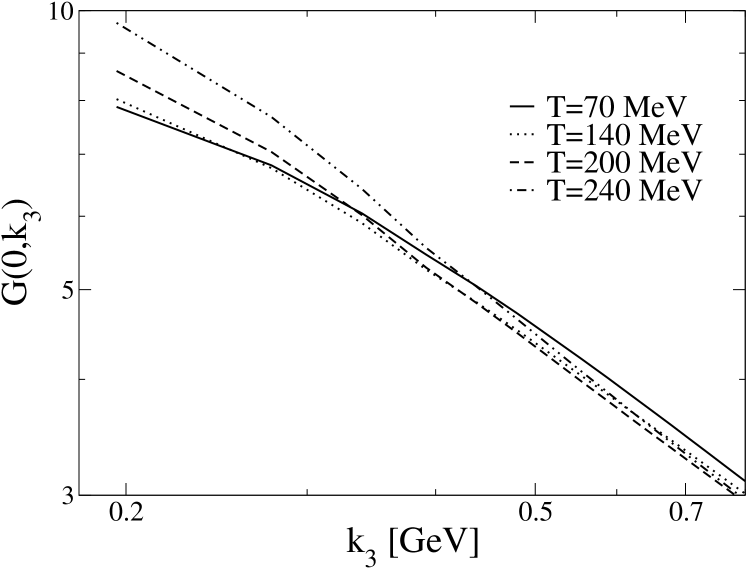
Figure 2: The ghost dressing function $G$ in the infrared region at different temperatures ($24^{3}$ momentum grid).

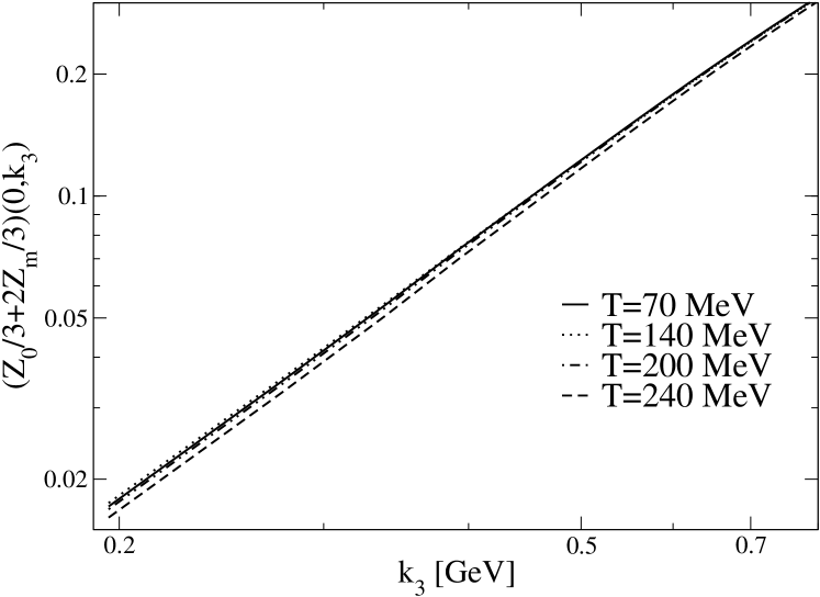
Figure 3: The averaged gluon dressing function $Z$ in the infrared region at different temperatures ($24^{3}$ momentum grid).

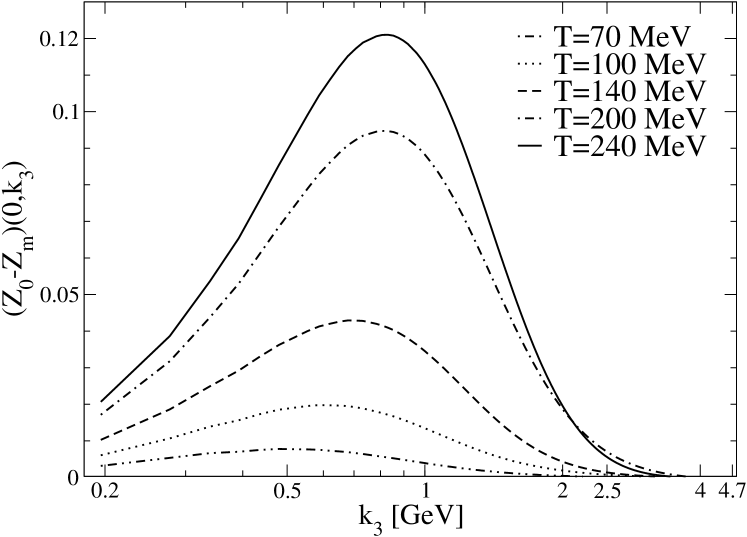
Figure 4: The difference $\Delta Z$ of the gluon dressing functions at different temperatures ($24^{3}$ momentum grid).

For the higher Matsubara modes the dressing functions have an interesting property: the combined gluon dressing $Z$ and the ghost dressing $G$ seem to depend only on the 4-momentum (at least approximately), while the higher modes of $\Delta Z$ are not $O(4)$ invariant, as expected (see figs. 5-7) .

Due to the numerical method, we are biased to stay in the confining phase. Nevertheless it is surprising that we find qualitatively similar solutions also for high temperatures. These solutions are numerically stable up to temperatures allowed by the UV cut-off, $2\pi T\approx\Lambda$. In order to draw conclusions on the character of the phase transition we need results from other numerical methods to support this finding. If so, our results would indicate a first order phase transition. Figs. 8 and 9 show that the changes of the ”wrong-phase” solutions with temperature are also smooth and are qualitatively the same as for small temperatures.

The running coupling $\alpha(k^{2})$, being a renormalization group invariant quantity, is of special interest. In Landau-gauge at zero temperature, a non-perturbative running coupling $\alpha(p^{2})$ can be defined via the relation:

$$\alpha(p^{2})=\alpha(\mu^{2})G^{2}(p^{2},\mu^{2})Z(p^{2},\mu^{2})\;.$$ (21)

In order to smoothly connect to the results for vanishing temperature we take for $Z$ the linear combination (12):

$$\alpha(n,p_{3}^{2},T):=\alpha(\mu^{2})G^{2}(n,p_{3}^{2},\mu^{2},T)Z(n,p_{3}^{2},\mu^{2},T).$$ (22)

As expected from the results for the dressing functions, the coupling (22) shows no temperature dependence beyond numerical uncertainties.

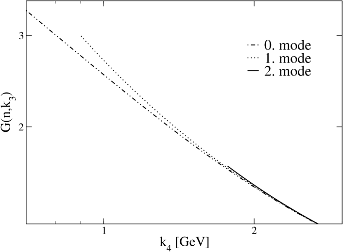
Figure 5: Different Matsubara modes of the ghost dressing function at $T=140$ MeV ($24^{3}$ momentum grid).

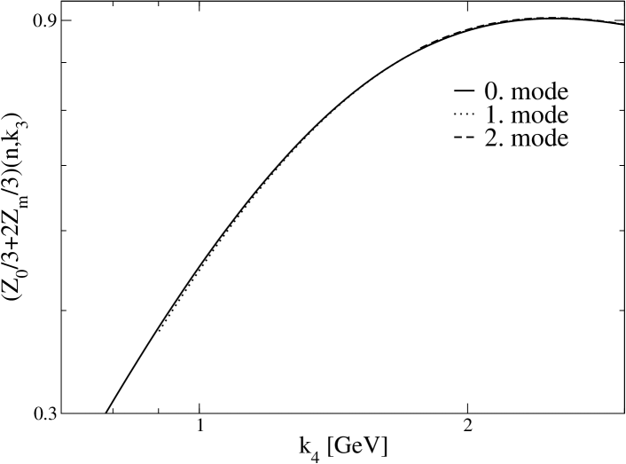
Figure 6: Different Matsubara modes of the averaged gluon dressing function $Z$ at $T=140$ MeV ($24^{3}$ momentum grid).

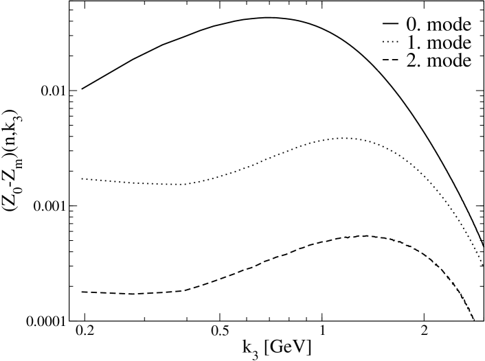
Figure 7: Different Matsubara modes of the difference $\Delta Z$ of the gluon dressing functions at $T=140$ MeV ($24^{3}$ momentum grid).

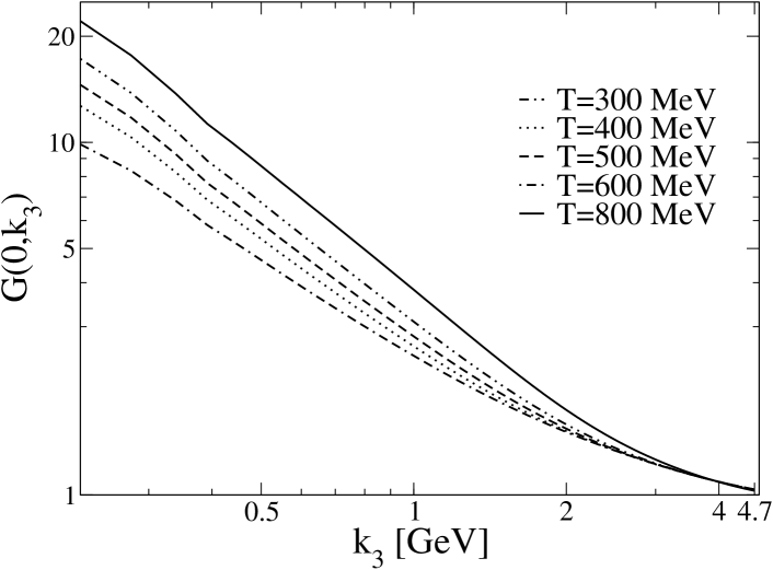
Figure 8: The ghost dressing function $G$ at high temperatures ($24^{3}$ momentum grid).

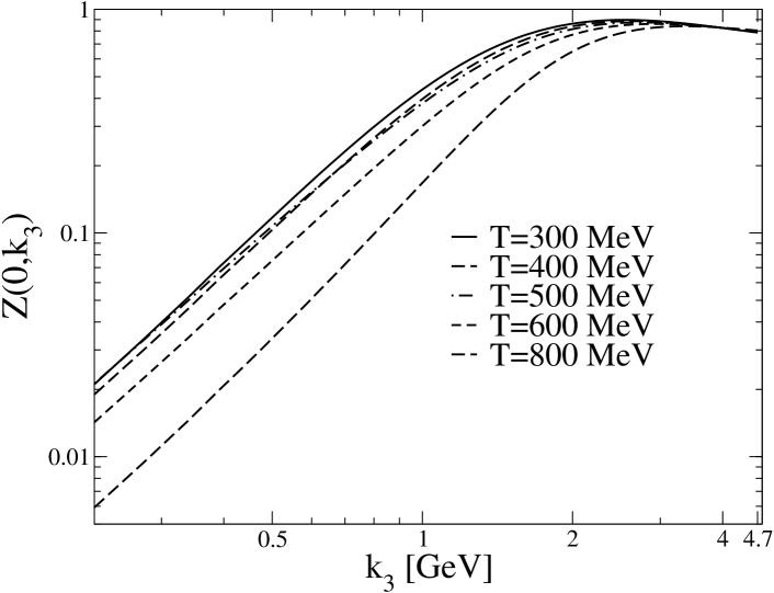
Figure 9: The averaged gluon dressing function $Z$ at high temperatures ($24^{3}$ momentum grid).

5 CJT Action and Phase Transition

$$V_{2}(D_{\mu\nu},D_{G}) =\;\frac{1}{2}\;\parbox{99.58464pt}{\psfig{width=99.58464pt}}\;-\frac{1}{12}\;\parbox{99.58464pt}{\psfig{width=99.58464pt}}$$

Figure 10: Diagrammatic representation of the two-loop contributions to the effective action.

$$V_{2}(D_{\mu\nu},D_{G}) =\frac{1}{3}\left(\parbox{99.58464pt}{\psfig{width=99.58464pt}}-1\right)\;-\frac{1}{6}\;\left(\parbox{99.58464pt}{\psfig{width=99.58464pt}}-1\right)$$

Figure 11: $V_{2}(D_{\mu\nu},D_{G})$ after inserting the reintegrated DSEs.

As we want to investigate the phase transition it is necessary to compute thermodynamic quantities. In order to do so, we need the temperature dependent effective action for vanishing fields and full propagators. Since we want to calculate the temperature dependence of different quantities, we need to assure energy conservation. Thus the DSEs, which we use to compute the dressing functions, have to be the variational equations of the energy functional, i.e. of the effective action. We take the known 2PI effective action by Cornwall, Jackiw and Tomboulis (CJT) Luttinger:1960ua for fully dressed propagators and bare vertices . First we discuss the action for vanishing temperature, given by the formula (c.f. ref. Haeri:hi )

$$V(D_{\mu\nu},D_{G}) =V_{0}(D_{\mu\nu},D_{G})+V_{2}(D_{\mu\nu},D_{G})\;,$$ (23)

$$V_{0}(D_{\mu\nu},D_{G}) =\int\frac{d^{4}p}{(2\pi)^{4}}{\rm Tr}\left\{\frac{1}{2}\left[{D^{0}_{\mu\alpha}}^{-1}(p)D_{\alpha\nu}(p)-\right.\right.$$

$$\left.g_{\mu\nu}\right]-\frac{1}{2}\ln\left({D^{0}_{\mu\alpha}}^{-1}(p)D_{\alpha\nu}(p)\right)-$$

$$\left[D_{G}^{0}(p)^{-1}D_{G}(p)-1\right]$$

$$+\ln\left(D_{G}^{0}(p)^{-1}D_{G}(p)\right)\Big{\}}\;,$$ (24)

where we already employed Euclidean space-time conventions.

In a truncation scheme with bare vertex functions only the diagrams of fig. 10 contribute to the effective action. For our truncation to the gluon propagator DSE, the 3-gluon vertex (10) is constructed from the dressing functions of the propagators. However, throughout this investigation we neglect variations of the vertex with respect to the gluon and ghost dressing functions, and thus employ

$$V_{2}(D_{\mu\nu},D_{G}) =\frac{1}{2}\int\frac{d^{4}p}{(2\pi)^{4}}\int\frac{d^{4}q}{(2\pi)^{4}}ip_{\mu}D_{\mu\nu}(p-q)$$

$$iq_{\mu}D_{G}(q)D_{G}(p)-\frac{1}{12}\int\frac{d^{4}p}{(2\pi)^{4}}\int\frac{d^{4}q}{(2\pi)^{4}}\Big{\{}$$

$$\Gamma^{0}_{\mu\rho\alpha}(p,-p-q,q)D_{\alpha\beta}(q)D_{\rho\sigma}(p+q)$$

$$\Gamma^{0}_{\beta\sigma\nu}(-q,p+q,-p)D_{\mu\nu}(p)\Big{\}}\;.$$ (25)

The variation of the action (23) with respect to the propagators reproduces the Dyson-Schwinger equations for the gluon and ghost propagators (6) and (5), however, with bare 3-gluon vertex. Multiplying the gluon DSE with the full gluon propagator and the ghost DSE with the full ghost propagator and performing the trace in colour and Lorentz indices and the integral in momentum space, we recover the two-loop diagrams of the CJT action. This results in:

$$V_{2}(D_{\mu\nu},D_{G}) =\int\frac{d^{4}p}{(2\pi)^{4}}{\rm Tr}\left\{-\frac{1}{6}\left[{D^{0}_{\mu\alpha}}^{-1}(p)D_{\alpha\nu}(p)-\right.\right.$$

$$\left.\delta_{\mu\nu}\right]+\frac{1}{3}\left[D_{G}^{0}(p)^{-1}D_{G}(p)-1\right]\Big{\}}\;,$$ (26)

see fig. 11 for a graphical representation. Inserting (26) and the explicit expression for the propagators in dependence on the dressing functions in (23) one obtains:

$$V(Z,G) =N_{C}\int\frac{d^{4}p}{(}2\pi)^{4}\Big{\{}$$

$$\left(Z_{3}Z(p^{2})-1\right)-\frac{3}{2}\ln\left(Z_{3}Z(p^{2})\right)$$

$$-\frac{2}{3}\left(\tilde{Z}_{3}G(p^{2})-1\right)+\ln\left(\tilde{Z}_{3}G(p^{2})\right)\Big{\}}.$$ (27)

For solving the corresponding DSEs numerically, we introduce a momentum cut-off $\Lambda$. Thus the renormalization constants $Z_{3}$ for the gluon wave function and $\tilde{Z}_{3}$ for the ghost propagator not only depend on the renormalization scale $\mu$ but also on the cut-off . Defining $x:=p^{2}$ one has:

$$V(Z,G) =\frac{N_{C}}{(4\pi)^{2}}\int_{0}^{\Lambda^{2}}dxx\Big{\{}\left(Z_{3}(\mu,\Lambda)Z(x,\mu)-1\right)$$

$$-\frac{3}{2}\ln\left(Z_{3}(\mu,\Lambda)Z(x,\mu)\right)$$

$$-\frac{2}{3}\left(\tilde{Z}_{3}(\mu,\Lambda)G(x,\mu)-1\right)$$

$$+\ln\left(\tilde{Z}_{3}(\mu,\Lambda)G(x,\mu)\right)\Big{\}}.$$ (28)

This quantity diverges like $\Lambda^{4}$, if the renormalization constants are only known to a finite accuracy. Furthermore, the three-gluon vertex is dressed by construction, which is not accounted for by the above action. In fact the following fit

$$f(x) =ax^{2}+c$$ (29)

to the cut-off dependence of the action yields:

$$a =-3.2\times 10^{-3}$$

$$c =(9.8\pm 1.3)\times 10^{-10}\textrm{GeV}^{4}$$ (30)

The result should be interpreted as vanishing of the effective action as the first term is of purely numerical origin and the second term is much too small to correspond to a scale of the system, $c^{\frac{1}{4}}\approx 5.6$ MeV.

At finite temperatures, the integral measure in eq. (27) has to be replaced by that for the space-time torus, see eq. (7). Furthermore, the finite temperature gluon propagator with its additional tensor structure (2) has to be inserted. Finally we get for the temperature dependent 1-particle irreducible CJT-Action:

$$V(T) =N_{C}T\sum_{n=-\infty}^{+\infty}\int\frac{d^{3}\vec{q}}{(2\pi)^{3}}\left\{\right.$$

$$\frac{2}{3}\left(Z_{3m}Z_{m}(\omega_{n},|\vec{p}|)-1\right)-\ln\left(Z_{3m}Z_{m}(\omega_{n},|\vec{p}|)\right)+$$

$$\frac{1}{3}\left(Z_{30}Z_{0}(\omega_{n},|\vec{p}|)-1\right)-\frac{1}{2}\ln\left(Z_{30}Z_{0}(\omega_{n},|\vec{p}|)\right)-$$

$$\frac{2}{3}\left(\tilde{Z}_{3}G(\omega_{n},|\vec{p}|)-1\right)+\ln\left(\tilde{Z}_{3}G(\omega_{n},|\vec{p}|)\right)\Big{\}}\;.$$ (31)

This effective action is temperature independent within numerical uncertainties up to $T=250$ MeV. For higher temperatures large variations are seen. Whether this is connected to the phase transition remains to be seen.

6 Conclusions

In this paper we have extended a truncation scheme for the Dyson-Schwinger equations of Yang-Mills theories in Landau-gauge to non-vanishing temperatures using the imaginary time formalism for quantum field theories in thermal equilibrium. We have obtained numerical solutions for the gluon and ghost propagators. Furthermore we have derived an expression for the CJT action of the interacting Yang-Mills theory, depending on dressed propagators.

The results can be summarised as follows: Temperature dependences of the ghost and gluon propagators are rather weak and the power-law behaviour in the infrared, already observed at vanishing temperature, persists. The corresponding CJT action vanishes (within numerical uncertainties) and does not possess any significant temperature dependence up to $T=250$ MeV. Thus gluons and ghost neither build up any pressure nor give raise to finite entropy of the system. An improved numerical method, especially one suitable for infinite volume, is, of course, desirable to study thermodynamic quantities below the phase transition. Corresponding investigations are currently performed.

Appendix

A Integral kernels for the DSEs

The complete algebraic expressions for the Lorentz structures that occur in the DSEs for the different products of dressing functions, are given here. First, there are the two kernels of the ghost equation (17):

$$A_{T}(k,q) =-\frac{\vec{k}^{2}\vec{q}^{2}-(\vec{k}\cdot\vec{q})^{2}}{(\vec{k}-\vec{q})^{2}}$$ (32)

$$A_{L}(k,q) =-\frac{k^{2}q^{2}-(kq)^{2}}{(k-q)^{2}}+\frac{\vec{k}^{2}\vec{q}^{2}-(\vec{k}\cdot\vec{q})^{2}}{(\vec{k}-\vec{q})^{2}}.$$ (33)

Secondly, the kernel of the ghost loop and the four kernels of the gluon loop for the heat-bath transversal part of the gluon equation (18):

$$R(k,q) =-\frac{\left(\vec{q}^{2}\vec{k}^{2}-(\vec{k}\cdot\vec{q})^{2}\right)}{\vec{k}^{2}}$$ (34)

$$M_{T}(k,q) =-2\frac{\vec{q}^{2}\vec{k}^{2}-(\vec{k}\cdot\vec{q})^{2}}{\vec{k}^{2}\vec{q}^{2}\vec{p}^{2}}\left((\vec{k}\cdot\vec{q})^{2}+\vec{k}^{2}\vec{q}^{2}+\right.$$

$$\left.2\vec{p}^{2}(\vec{k}^{2}+\vec{q}^{2})\right)$$ (35)

$$M_{1}(k,q) =-2\frac{\left(q_{0}\vec{k}\cdot\vec{q}-k_{0}\vec{q}^{2}\right)^{2}\left((\vec{k}\cdot\vec{p})^{2}+\vec{k}^{2}\vec{p}^{2}\right)}{\vec{k}^{2}\vec{q}^{2}\vec{p}^{2}q^{2}}$$ (36)

$$M_{2}(k,q) =-2\frac{\left(p_{0}\vec{k}\cdot\vec{p}-k_{0}\vec{p}^{2}\right)^{2}\left((\vec{k}\cdot\vec{q})^{2}+\vec{k}^{2}\vec{q}^{2}\right)}{\vec{k}^{2}\vec{q}^{2}\vec{p}^{2}p^{2}}$$ (37)

$$M_{L}(k,q) =-2\frac{\left(\vec{q}^{2}\vec{k}^{2}-(\vec{k}\cdot\vec{q})^{2}\right)\left(q^{2}p^{2}-q_{0}p_{0}qp\right)^{2}}{\vec{k}^{2}\vec{q}^{2}\vec{p}^{2}k^{2}p^{2}}.$$ (38)

And third the corresponding kernels for the heat-bath longitudinal part (19):

$$P(k,q) =-\frac{\left(q_{0}\vec{k}^{2}-k_{0}\vec{k}\cdot\vec{q}\right)^{2}}{k^{2}\vec{k}^{2}}$$ (39)

$$N_{T}(k,q) =-2\frac{\left(k_{0}\vec{k}\cdot\vec{q}-q_{0}\vec{k}^{2}\right)^{2}\left((\vec{q}\cdot\vec{p})^{2}+\vec{q}^{2}\vec{p}^{2}\right)}{\vec{k}^{2}\vec{q}^{2}\vec{p}^{2}k^{2}}$$ (40)

$$N_{1}(k,q) =-2\frac{\left(\vec{q}^{2}\vec{k}^{2}-(\vec{k}\cdot\vec{q})^{2}\right)\left(k^{2}q^{2}-k_{0}q_{0}kq\right)^{2}}{\vec{k}^{2}\vec{q}^{2}\vec{p}^{2}k^{2}p^{2}}$$ (41)

$$N_{2}(k,q) =-2\frac{\left(\vec{q}^{2}\vec{k}^{2}-(\vec{k}\cdot\vec{q})^{2}\right)\left(k^{2}p^{2}-k_{0}p_{0}kp\right)^{2}}{\vec{k}^{2}\vec{q}^{2}\vec{p}^{2}k^{2}q^{2}}$$ (42)

$$N_{L}(k,q) =-\frac{1}{2\vec{k}^{2}\vec{q}^{2}\vec{p}^{2}k^{2}q^{2}p^{2}}\left[(\vec{p}\cdot\vec{k})\vec{q}^{2}\left(k_{0}p^{2}+p_{0}k^{2}\right)-\right.$$

$$\left.(\vec{p}\cdot\vec{q})\vec{k}^{2}\left(p_{0}q^{2}+q_{0}p^{2}\right)+\right.$$

$$\left.(\vec{k}\cdot\vec{q})\vec{p}^{2}\left(k_{0}q^{2}-q_{0}k^{2}\right)\right]^{2}.$$ (43)

B Finite size effects

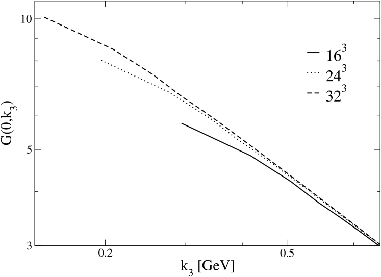
Figure 12: The ghost dressing function $G$ at $T=140$ MeV on different momentum grids.

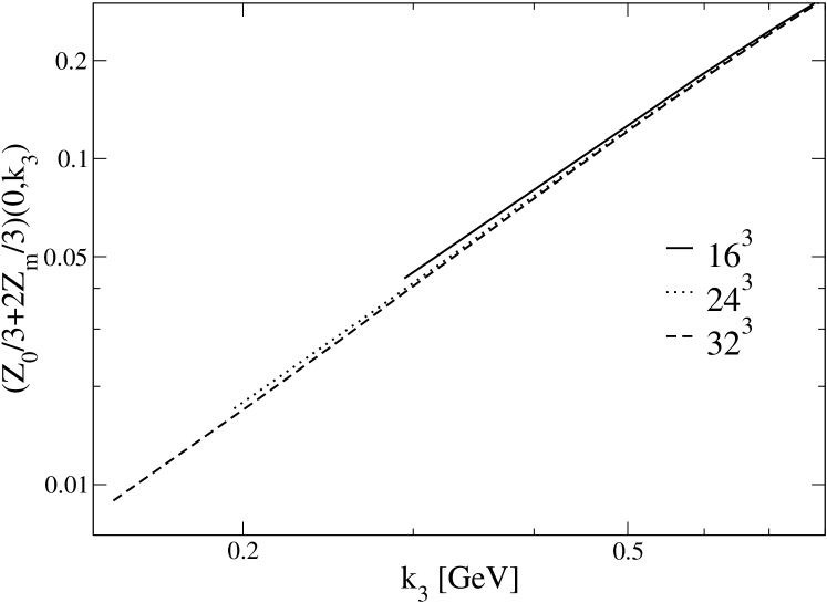
Figure 13: The averaged gluon dressing function $Z$ at $T=140$ MeV on different momentum grids.

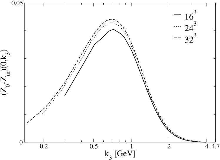
Figure 14: The difference $\Delta Z$ of the gluon dressing functions at $T=140$ MeV on different momentum grids.

As expected, finite-size effects cannot be neglected completely but are rather small and change the results only in a quantitative way, as can be seen from the figures 12 - 14. The deviations tend to increase for higher temperatures, since the ultraviolet cutoff is rather low ($4.7$ GeV). Finite size effects do not alter our conclusions. Especially, the temperature estimate of eq. (8) is fairly independent of the finite-momentum lattice size.

References

- (1) F. Karsch and E. Laermann, arXiv:hep-lat/0305025; and references therein.
- (2) R. Alkofer and L. von Smekal, Phys. Rept. 353 (2001) 281 [arXiv:hep-ph/0007355].
- (3) C. D. Roberts and S. M. Schmidt, Prog. Part. Nucl. Phys. 45 (2000) S1 [arXiv:nucl-th/0005064].
- (4) L. von Smekal and R. Alkofer, Proceedings of the Fourth International Conference on Quark Confinement and the Hadron Spectrum (CONFINEMENT IV), July 3-8, Vienna, [arXiv:hep-ph/0009219]; R. Alkofer and L. von Smekal, Proceedings of the Conference ”Quark Nuclear Physics 2000”, Adelaide, Feb. 21 - 25, 2000, Nucl. Phys. A 680 (2000) 133 [arXiv:hep-ph/0004141].
- (5) F. D. Bonnet et al., Phys. Rev. D 64 (2001) 034501 [arXiv:hep-lat/0101013].
- (6) J. M. Pawlowski, D. F. Litim, S. Nedelko and L. von Smekal, Phys. Rev. Lett., in print, arXiv:hep-th/0312324; C. S. Fischer and H. Gies, arXiv:hep-ph/0408089.
- (7) C. S. Fischer and R. Alkofer, Phys. Rev. D 67 (2003) 094020 [arXiv:hep-ph/0301094].
- (8) C. S. Fischer, PhD thesis, Universität Tübingen, 2003, arXiv:hep-ph/0304233.
- (9) T. Kugo and I. Ojima, Prog. Theor. Phys. Suppl. 66 (1979) 1.
- (10) D. Zwanziger, Nucl. Phys. B 323 (1989) 513.
- (11) D. Zwanziger, Phys. Rev. D 69 (2004) 016002 [arXiv:hep-ph/0303028].
- (12) V. N. Gribov, Nucl. Phys. B139 (1978) 1.
- (13) A. Maas, J. Wambach, B. Gruter and R. Alkofer, Eur. Phys. J. C in print, arXiv:hep-ph/0408074.
- (14) J. M. Luttinger and J. C. Ward, Phys. Rev. 118 (1960) 1417. J. M. Cornwall, R. Jackiw and E. Tomboulis, Phys. Rev. D 10 (1974) 2428.
- (15) B. J. Haeri, Phys. Rev. D 48 (1993) 5930 [arXiv:hep-ph/9309224].
- (16) J. I. Kapusta, Finite-temperature field theory (Cambridge University Press, Cambridge, 1993).
- (17) M. L. Bellac, Thermal Field Theory (Cambridge University Press, Cambridge, 1996).
- (18) J. C. Taylor, Nucl. Phys. B 33 (1971) 436.
- (19) P. Watson and R. Alkofer, Phys. Rev. Lett. 86 (2001) 5239 [arXiv:hep-ph/0102332]; R. Alkofer, L. von Smekal and P. Watson, arXiv:hep-ph/0105142.
- (20) C. Lerche and L. von Smekal, Phys. Rev. D 65 (2002) 125006 [arXiv:hep-ph/0202194].
-
(21)
L. von Smekal, R. Alkofer and A. Hauck,
Phys. Rev. Lett. 79 (1997) 3591
[arXiv:hep-ph/9705242];
L. von Smekal, A. Hauck and R. Alkofer, Annals Phys. 267 (1998) 1 [arXiv:hep-ph/9707327];
A. Hauck, L. von Smekal and R. Alkofer, Comput. Phys. Commun. 112 (1998) 166 [arXiv:hep-ph/9804376]. - (22) C. S. Fischer, R. Alkofer and H. Reinhardt, Phys. Rev. D 65 (2002) 094008 [arXiv:hep-ph/0202195].
- (23) R. Alkofer, C. S. Fischer and F. J. Llanes-Estrada, Phys. Lett. B 611 (2005) 279 [arXiv:hep-th/0412330].
- (24) W. Schleifenbaum, A. Maas, J. Wambach and R. Alkofer, arXiv:hep-ph/0411052.
- (25) A. Cucchieri, T. Mendes and A. Mihara, JHEP 0412 (2004) 012 [arXiv:hep-lat/0408034].
- (26) P. O. Bowman, U. M. Heller, D. B. Leinweber, M. B. Parappilly and A. G. Williams, Phys. Rev. D 70 (2004) 034509 [arXiv:hep-lat/0402032]; O. Oliveira and P. J. Silva, arXiv:hep-lat/0410048.
- (27) N. Brown and M. R. Pennington, Phys. Rev. D 38 (1988) 2266.
- (28) J. Berges, [arXiv:hep-ph/0401172]; M. E. Carrington, Eur. Phys. J. C 35 (2004) 383 [arXiv:hep-ph/0401123]; M. E. Carrington, G. Kunstatter and H. Zaraket, [arXiv:hep-ph/0309084]. A. Arrizabalaga and J. Smit, Phys. Rev. D 66 (2002) 065014 [arXiv:hep-ph/0207044].