Collisional Energy Loss of a Heavy Quark in an Anisotropic Quark-Gluon Plasma

Abstract

We compute the leading-order collisional energy loss of a heavy quark propagating through a quark-gluon plasma in which the quark and gluon distributions are anisotropic in momentum space. Following the calculation outlined for QED in an earlier work we indicate the differences encountered in QCD and their effect on the collisional energy loss results. For a 20 GeV bottom quark we show that momentum space anisotropies can result in the collisional heavy quark energy loss varying with the angle of propagation by up to 50%. For low velocity quarks we show that anisotropies result in energy gain instead of energy loss with the energy gain focused in such a way as to accelerate particles along the anisotropy direction thereby reducing the momentum-space anisotropy. The origin of this negative energy loss is explicitly identified as being related to the presence of plasma instabilities in the system.

I Introduction

An understanding of the production, propagation, and hadronization of heavy quarks in relativistic heavy-ion collisions is important for predicting a number of experimental observables including the heavy-meson spectrum, the single lepton spectrum, and the dilepton spectrum. The first experimental results for the inclusive electron spectrum have been reported adcox:2002 in addition to the first measurements of $J/\psi$ production at RHIC nagle:2002 . The measurement of the inclusive electron spectrum allows for a determination of heavy quark energy loss since it is primarily due to the semi-leptonic decay of charm quarks. The heavy quark energy loss comes into play since it is necessary in order to predict the heavy quark energy at the decay point. It is therefore important to have a thorough theoretical understanding of heavy quark energy loss for a proper comparison with the experimental results. In this paper we will show that in QCD there is a modification of the leading-order (collisional) heavy quark energy loss if there is a momentum-space anisotropy in the underlying quark and gluon distribution functions.

Here we will focus on the collisional energy loss using the techniques of Braaten and Thoma Braaten:1991jj ; Braaten:1991we which have been extended to anisotropic systems in Ref. Romatschke:2003vc . For a review of the radiative energy loss in isotropic systems see Refs. Baier:2000mf and Accardi:2003gp . The method employed by Braaten and Thoma gives the complete result for the collisional energy loss by considering independently the contributions from soft (involving momenta $q\sim m_{D}$) and hard ($q\sim T$) gluon exchange. The two scales, $m_{D}$ and $T$, are then separated by an arbitrary momentum scale $q^{*}$ which cuts off the UV and IR divergences in the soft and hard contributions, respectively. Moreover, it was found that in the weak-coupling or high-temperature limit $\alpha_{s}\ll 1$ the condition $m_{D}\ll q^{*}\ll T$ could be used to expand the resulting integral expressions for the soft and hard contributions further, giving an analytic result for the energy loss independent of the separation scale $q^{*}$ Braaten:1991jj ; Braaten:1991we . However, in the case of QCD at temperatures accessible by heavy-ion collision experiments the coupling constant is quite large ($\alpha_{s}\sim 0.2-0.3$) and as a consequence the analytic expression of Braaten and Thoma can give unphysical results for the energy loss as we will demonstrate.

On the good news side, it turns out that when one does not expand the integral expressions with respect to the condition $m_{D}\ll q^{*}\ll T$ the isotropic contributions to the energy loss always stay positive, even for very large coupling, as has been shown for QED Romatschke:2003vc . However, this comes at the expense of giving up independence of the complete result on the scale $q^{*}$, which then has to be fixed somehow. Fortunately, it turns out that in the weak-coupling limit this scale dependence becomes very small and as a consequence, unless $q^{*}$ is taken to be very large ($q^{*}\gg T$) or very small ($q^{*}\ll m_{D}$), one recovers the analytic results found by Braaten and Thoma. When the coupling is increased one can then still fix $q^{*}$ by the “principle of minimal sensitivity”, which means that $q^{*}$ is chosen such that the energy loss (and therefore also the variation with respect to $q^{*}$) is minimized. In addition, the principle of minimal sensitivity provides a way to estimate the theoretical uncertainty of the result by varying $q^{*}$ by a fixed amount around the point at which the energy loss is least sensitive to this scale.

The main reason why a calculation of this type is important to perform is that the presence of plasma instabilities Weibel:1959 ; Mrowczynski:1993qm ; Mrowczynski:1994xv ; Mrowczynski:1997vh ; Randrup:2003cw ; Romatschke:2003ms ; Romatschke:2003vc ; Arnold:2003rq ; Mrowczynski:2004mr ; Romatschke:2003yc ; Romatschke:2004jh ; Arnold:2004al in anisotropic systems could have a significant effect on observables like the heavy quark energy loss. In fact, the presence of such instabilities naively renders the calculation of the soft part divergent; however, there is protection mechanism dubbed “dynamical shielding” which renders the collisional energy loss finite for QED Romatschke:2003vc . This protection mechanism trivially extends to the case of QCD since the only thing that changes in going from soft QED to soft QCD at leading-order is the numerical value of the Debye mass. However, at large coupling the presence of instabilities and associated poles on unphysical Riemann sheets Romatschke:2004jh causes significant changes in the soft energy loss contribution for both QED and QCD. In fact, as we will discuss, the unphysical poles can even change the sign of the heavy quark energy loss at low momentum turning it instead into energy gain.

The paper is organized as follows: In Sec. II we review the calculation of the collisional energy loss including the case of very strong anisotropies. In Sec. III we discuss the role that modes on the unphysical sheets play in the calculation. In Sec. IV we present results for the collisional energy loss of a heavy quark for isotropic and anisotropic systems. We give our conclusions in Sec. V.

II Collisional energy loss in QCD

Following Refs. Braaten:1991jj ; Braaten:1991we ; Romatschke:2003vc ; Romatschke:2003yc the collisional energy loss of a heavy quark with velocity v is divided into a soft contribution and a hard contribution. The soft contribution within QCD has exactly the same form as in QED except that the expression for the Debye mass is different and there is an overall Casimir which has to be taken into account. Therefore the soft contribution from Ref. Romatschke:2003vc can be taken directly and only needs to be rescaled appropriately. The hard contribution in QCD is, however, different for two reasons: a new gluon scattering diagram appears due to the three-gluon coupling and the graphs which are topologically equivalent to the QED fermion-photon graphs no longer cancel due to non-trivial Casimir invariants. In the next two subsections we present explicit integral expressions for both the soft and hard contributions to the energy loss in the limit of infinite quark mass. In the final subsection we discuss how the limit of infinite anisotropy can be taken.

II.1 Soft contribution

The soft contribution in the case of QCD is given by the expression

$$-\left({{\rm d}W\over{\rm d}t}\right)_{\rm soft}={\mathcal{Q}}^{2}\;{\rm Im}\int\!{d^{3}{\bf q}\over(2\pi)^{3}}\,({\bf q}\cdot{\bf v})\,v^{i}\left[\Delta^{ij}(Q)-\Delta^{ij}_{0}(Q)\right]v^{j}\;,$$ (1)

where ${\mathcal{Q}}$ is the quark color charge in the fundamental representation with ${\mathcal{Q}}^{2}=g^{2}(N_{c}^{2}-1)/(2N_{c})$ and the two propagators $\Delta^{ij}(Q)$ and $\Delta^{ij}_{0}(Q)$ denote the hard-loop and free gluon propagators, respectively. The hard-loop gluon propagator in an anisotropic system has been calculated in Ref. Romatschke:2003ms and can be expressed as

$${\bf\Delta}(Q)=\Delta_{A}(Q)\,[{\bf A}-{\bf C}]+\Delta_{G}(Q)\,[(q^{2}-\omega^{2}+\alpha+\gamma){\bf B}+(\beta-\omega^{2}){\bf C}-\delta{\bf D}]\;,$$ (2)

where the tensor basis for the spacelike components of a system with one preferred direction specified by $\hat{\bf n}$ is: $A^{ij}=\delta^{ij}-k^{i}k^{j}/k^{2}$, $B^{ij}=k^{i}k^{j}/k^{2}$, $C^{ij}=\tilde{n}^{i}\tilde{n}^{j}/\tilde{n}^{2}$, $D^{ij}=k^{i}\tilde{n}^{j}+k^{j}\tilde{n}^{i}$ with $\tilde{n}^{i}=A^{ij}n^{j}$. The propagators $\Delta_{A}$ and $\Delta_{G}$ are then given by

$$\Delta_{A}^{-1}(Q) = q^{2}-\omega^{2}+\alpha\;,$$

$$\Delta_{G}^{-1}(Q) = (q^{2}-\omega^{2}+\alpha+\gamma)(\beta-\omega^{2})-q^{2}\tilde{n}^{2}\delta^{2}\;,$$ (3)

with $\alpha$, $\beta$, $\gamma$, and $\delta$ being the hard-loop gluon structure functions. Except for some special cases (certain angles of propagation, infinite anisotropy, etc.), the analytic expressions for the structure functions are quite complicated in form and it is more convenient to use a numerical evaluation of their integral representations Romatschke:2003ms .

The structure functions of anisotropic systems depend on the precise form of the quark and gluon distribution functions. Here we will assume that the distribution function is spatially homogeneous and therefore given by

$$f({\bf p})\equiv 2N_{f}\left(n({\bf p})+\bar{n}({\bf p})\right)+4N_{c}n_{g}({\bf p})\;,$$ (4)

where $n$, $\bar{n}$, and $n_{g}$ are the distribution functions of quarks, anti-quarks, and gluons, respectively. We will further assume that the anisotropic distribution function, $f({\bf p})$, can be obtained from an isotropic distribution function by rescaling one direction in momentum space

$$f({\bf p})=N(\xi)\,f_{\rm iso}\left(p\sqrt{1+\xi(\hat{\bf p}\cdot\hat{\bf n})^{2}}\right)\,,$$ (5)

where $N(\xi)=\sqrt{1+\xi}$ is a normalization constant with $\xi$ the strength of the anisotropy. The anisotropy strength $\xi$ is in the range $-1<\xi<\infty$ with $\xi=0$ corresponding to the original isotropic distribution. In order to simplify the analysis we take quarks and gluons to have the same anisotropy parameter although in general they can be different. Even though its effects might be interesting, different anisotropies for quarks and gluons will not be studied in this paper.

The soft contribution to the collisional energy loss of a heavy quark in an anisotropic quark-gluon plasma is then given by

$$-\left({{\rm d}W\over{\rm d}x}\right)_{\rm soft}\!\!\!\!\!\!\! = \!\!\!\frac{{\mathcal{Q}}^{2}}{v}\,{\rm Im}\,\int{d\Omega_{q}\over(2\pi)^{3}}\,\frac{\hat{\omega}}{(1-\hat{\omega}^{2})}\,\Biggl{[}-\alpha\frac{(v^{2}-\hat{\omega}^{2}-{(\tilde{\bf n}\cdot{\bf v})^{2}\over\tilde{n}^{2}})}{2(1-\hat{\omega}^{2})}\ln{\frac{q^{*2}(1-\hat{\omega}^{2})+\alpha}{\alpha}}$$ (6)

$$\hskip 156.49014pt+F(q^{\star})-F(0)\Biggr{]}\,,$$

where

$$F(q)=\frac{\mathcal{A}}{4\mathcal{C}}\ln{\left(-4\mathcal{C}\left(\mathcal{C}q^{4}+\mathcal{D}q^{2}+\mathcal{E}\right)\right)}+\frac{\mathcal{AD}-2\mathcal{BC}}{4\mathcal{C}\sqrt{\mathcal{D}^{2}-4\mathcal{CE}}}\ln{\frac{\sqrt{\mathcal{D}^{2}-4\mathcal{CE}}+\mathcal{D}+2\mathcal{C}q^{2}}{\sqrt{\mathcal{D}^{2}-4\mathcal{CE}}-\mathcal{D}-2\mathcal{C}q^{2}}}\;,$$ (7)

with

$$\mathcal{A} = (1-\hat{\omega}^{2})^{2}\beta+\hat{\omega}^{2}{(\tilde{\bf n}\cdot{\bf v})^{2}\over\tilde{n}^{2}}(\alpha+\gamma)-2\hat{\omega}(1-\hat{\omega}^{2})(\tilde{\bf n}\cdot{\bf v})\hat{\delta}\;,$$

$$\mathcal{B} = \left((\alpha+\gamma)\beta-\tilde{\bf{n}}^{2}\hat{\delta}^{2}\right)(1-\hat{\omega}^{2}-{(\tilde{\bf n}\cdot{\bf v})^{2}\over\tilde{n}^{2}})\;,$$

$$\mathcal{C} = -\hat{\omega}^{2}(1-\hat{\omega}^{2})\;,$$

$$\mathcal{D} = -\hat{\omega}^{2}(\alpha+\gamma)+(1-\hat{\omega}^{2})\beta\;,$$

$$\mathcal{E} = (\alpha+\gamma)\beta-\tilde{\bf{n}}^{2}\hat{\delta}^{2}\;,$$ (8)

and $\hat{\omega}={\bf\hat{q}}\cdot{\bf v}$, and $\hat{\delta}=q\delta$. In order to regulate the soft contribution it is necessary to introduce a UV momentum cutoff $q^{*}$ on the $q$ integration.

Note that in the case of an anisotropic system unstable modes are present that manifest themselves as potentially unregulated poles of the propagator in the static limit. However, as discussed in our previous paper Romatschke:2003vc the mechanism of “dynamical shielding” protects the collisional energy loss from these potentially devastating singularities in the soft contribution. These singularities could arise in terms containing, for example, $(q^{2}+\alpha)^{-1}$, due to the fact that in the static limit the structure function $\alpha$ is negative-valued. However, if one takes the static limit of $\alpha$ carefully we find

$$\lim_{\omega\rightarrow 0}\alpha(\omega,q)=M^{2}(-1+iD\hat{\omega})+{\cal O}(\omega^{2})\;,$$ (9)

where $M$ and $D$ depend on the angle of propagation with respect to the anisotropy vector and the strength of the anisotropy. As long as $D$ is non-vanishing the singularities are regularized because of the $\hat{\omega}$ in the numerator of Eq. (1) and we call the singularity “dynamically shielded”. A proof of dynamical shielding for very weak and strong anisotropies can be found in Refs. Romatschke:2003vc and Romatschke:2003yc .

In the isotropic limit ($\xi=0$) Eq. (6) corresponds to the result of Thoma and Gyulassy Thoma:1991fm and one obtains the soft contribution found by Braaten and Thoma Braaten:1991we when expanding Eq. (6) under the additional assumption $q^{*}\gg m_{D}$ Romatschke:2003yc . The effect of this expansion is that the result of Ref. Braaten:1991we becomes negative for small $q^{*}/m_{D}$ (but allows the calculation of an analytic result for the isotropic collisional energy loss) while the unexpanded result is positive for all $q^{*}/m_{D}$.

II.2 Hard Contribution

The hard contribution can be separated into two parts: one contribution coming from the scattering of the heavy quark on quarks in the plasma and another that takes into account the scattering on plasma gluons (corresponding to the tree-level diagrams shown in Fig. 1). Assuming the velocity of the quark to be much higher then the ratio of the plasma temperature to the energy of the quark, $v\gg T/E$, the contribution coming from quark-quark scattering can be reduced to Braaten:1991we

$$-\left({\rm d}W\over{\rm d}x\right)_{\rm hard}^{Qq}\!\! = {2(4\pi)^{3}N_{f}\alpha_{s}^{2}\over 3v}\int{d^{3}{\bf k}\over(2\pi)^{3}}{n({\bf k})\over k}\int{d^{3}{\bf k^{\prime}}\over(2\pi)^{3}}{1-n({\bf k}^{\prime})\over k^{\prime}}\delta(\omega-{\bf v}\cdot{\bf q})$$ (10)

$$\times\;\Theta(q-q^{*}){\omega\over(\omega^{2}-q^{2})^{2}}\left[2(k-{\bf v}\cdot{\bf k})^{2}+{1-v^{2}\over 2}(\omega^{2}-q^{2})\right],\;$$

after performing the Dirac traces and evaluating the sum over spins. The contribution coming from quark-gluon scattering gives

$$-\left({\rm d}W\over{\rm d}x\right)_{\rm hard}^{Qg}\!\! = {(4\pi)^{3}\alpha_{s}^{2}\over 2v}\int{d^{3}{\bf k}\over(2\pi)^{3}}{n_{g}({\bf k})\over k}\int{d^{3}{\bf k^{\prime}}\over(2\pi)^{3}}{1+n_{g}({\bf k}^{\prime})\over k^{\prime}}\delta(\omega-{\bf v}\cdot{\bf q})\Theta(q-q^{*})$$ (11)

$$\times\;\omega\left[\frac{(1-v^{2})^{2}}{(k-{\bf v}\cdot{\bf k})^{2}}+8\frac{(k-{\bf v}\cdot{\bf k})^{2}+\frac{1-v^{2}}{2}(\omega^{2}-q^{2})}{(\omega^{2}-q^{2})^{2}}\right].\quad$$

Here $n({\bf k})$ and $n_{g}({\bf k})$ are the anisotropic versions of the tree-level Fermi-Dirac and Bose-Einstein distribution functions at zero chemical potential specified in Eq. (4), $\omega=k^{\prime}-k$, and ${\bf q}={\bf k}^{\prime}-{\bf k}$. Note also that $q^{*}$ acts as an IR cutoff for the $q$ integration. Since the integrand is odd under the interchange ${\bf k}\leftrightarrow{\bf k}^{\prime}$ the terms involving the products $n({\bf k})n({\bf k}^{\prime})$ and $n_{g}({\bf k})n_{g}({\bf k}^{\prime})$ vanish since they are symmetric. Following Ref. Romatschke:2003vc , some of the integrations can be performed giving

Figure 1: Tree-level Feynman diagrams for the scattering processes $Qq\rightarrow Qq$ (first diagram) and $Qg\rightarrow Qg$ (remaining diagrams).

$$-\left({\rm d}W\over{\rm d}x\right)_{\rm hard}^{Qq} \!\!\!=\!\! {8\alpha_{s}^{2}N_{f}(\hat{q}^{*})^{2}T^{2}\sqrt{1+\xi}\over 3\pi^{3}v}\int_{0}^{\infty}z\,dz\int_{-1}^{1}d\cos\theta_{k}\left[\int_{0}^{2\pi}\!d\phi_{k}F_{1}(x)\right]$$

$$\times\int_{-1}^{1}d\cos{\theta_{q}}\;{\mathcal{T}}{v\cos\theta_{q}\over(v^{2}\cos^{2}\theta_{q}-1)^{2}}\left[2z^{2}(1-v\cos\theta_{k})^{2}+{1-v^{2}\over 2}(v^{2}\cos^{2}\theta_{q}-1)\right],$$

$$-\left({\rm d}W\over{\rm d}x\right)_{\rm hard}^{Qg} \!\!\!=\!\! {2\alpha_{s}^{2}(\hat{q}^{*})^{2}T^{2}\sqrt{1+\xi}\over\pi^{3}v}\int_{0}^{\infty}z\,dz\int_{-1}^{1}d\cos\theta_{k}\left[\int_{0}^{2\pi}\!d\phi_{k}F_{2}(x)\right]$$

$$\times\int_{-1}^{1}d\cos{\theta_{q}}\;{\mathcal{T}}v\cos\theta_{q}\left[\frac{(1-v^{2})^{2}}{z^{2}(1-v\cos\theta_{k})^{2}}+8\frac{z^{2}(1-v\cos\theta_{k})^{2}+\frac{1-v^{2}}{2}(v^{2}\cos^{2}\theta_{q}-1)}{(v^{2}\cos^{2}\theta_{q}-1)^{2}}\right],$$

where ${\mathcal{T}}$ denotes the unwieldy expression

$${\mathcal{T}}=\Theta(z+v\cos{\theta_{q}})\frac{\Theta(4z^{2}\sin^{2}\theta_{k}\sin^{2}\theta_{q}-(1-v^{2}\cos^{2}\theta_{q}+2\cos\theta_{q}z(\cos\theta_{k}-v))^{2})}{\sqrt{4z^{2}\sin^{2}\theta_{k}\sin^{2}\theta_{q}-(1-v^{2}\cos^{2}\theta_{q}+2\cos\theta_{q}z(\cos\theta_{k}-v))^{2}}},$$ (13)

and

$$F_{1}(x) = \frac{1}{x^{2}T^{2}}\int_{xT}^{\infty}dq\,q\ n(q)=\frac{x\ln(1+\exp{(-x)})-{\rm Li}_{2}(-\exp{(-x)})}{x^{2}}$$

$$F_{2}(x) = \frac{1}{x^{2}T^{2}}\int_{xT}^{\infty}dq\,q\ n_{g}(q)=\frac{-x\ln(1-\exp{(-x)})+{\rm Li}_{2}(\exp{(-x)})}{x^{2}}\,,$$ (14)

where $x=q^{*}z\sqrt{1+\xi(n_{x}\sin\theta_{k}\cos\phi_{k}+n_{z}\cos\theta_{k})^{2}}/T$, with $n_{z}=\bf{\hat{n}}\cdot\hat{\bf v}$ and $1=n_{x}^{2}+n_{z}^{2}$. The remaining integrations have to be performed numerically.

Similar to what has been found for the soft part, in the isotropic limit the hard contribution becomes that of Braaten and Thoma Braaten:1991we when expanding Eq. (LABEL:myelosshard3) with respect to $q^{*}\ll T$; also, the expanded result becomes negative for large $q^{*}/T$, while the unexpanded result is always positive in the isotropic limit.

II.3 Very strong anisotropies

There are however a few special cases where the structure functions become quite simple, notably the extreme anisotropy limit, $\xi\rightarrow\infty$, which corresponds to the parton distribution function having the form

$$f({\bf p})=F(p_{\perp})\delta(p_{z})\,.$$ (15)

The resulting expressions for the structure functions have been calculated in Ref. Romatschke:2003yc and this special case has been treated in more detail in a separate publication Romatschke:2004jh . Using these structure functions one is able to calculate the soft contribution to the energy loss in the large $\xi$ case by evaluation of Eq. (6). However, in the extreme limit $\xi\rightarrow\infty$ this is complicated by the presence of troublesome spacelike quasiparticle modes Romatschke:2004jh . For large but finite $\xi$ these modes are integrable because they move off the physical sheet onto the neighboring unphysical sheets but for $\xi=\infty$ they result in a pole in the integrand that needs to be regulated. Fortunately, a natural regularization is provided by the fact that for any finite $\xi$, these modes are outside of the physical spectrum; therefore, when keeping $\xi$ finite and sending it to infinity only after having done the integrations, one is able to produce well-defined results.

The hard contribution in the large $\xi$ case is easily found by using Eq. (LABEL:myelosshard3) together with

$$\lim_{\xi\rightarrow\infty}\sqrt{1+\xi}\,F_{1}\left(\hat{q}^{*}z\sqrt{1+\xi(\hat{k}\cdot\hat{n})^{2}}\right)=\delta(\hat{k}\cdot\hat{n})\int_{-\infty}^{\infty}dy\,F_{1}(\hat{q}^{*}z\sqrt{1+y^{2}})$$ (16)

and similarly for $F_{2}$. Using

$$\hat{k}\cdot\hat{n}=n_{x}\sin{\theta_{k}}\cos{\phi_{k}}+n_{z}\cos{\theta_{k}}\,,$$ (17)

the delta function can be cast into the form

$$\delta(\hat{k}\cdot\hat{n})=\frac{\delta(\phi_{k}-\phi_{0})}{\sqrt{n_{x}^{2}\sin^{2}{\theta_{k}}-n_{z}^{2}\cos^{2}{\theta_{k}}}}\,,$$ (18)

with

$$n_{x}\cos\phi_{0}=-n_{z}{\rm cot}\theta_{k}\,.$$ (19)

Using the symmetry $2\pi-\phi\leftrightarrow\phi$ and substituting $\cos{\theta_{k}}\rightarrow n_{x}\cos{\theta_{k}}$ the remaining integrations are easily implemented.

III Effects of modes on the unphysical sheet

In a previous paper we have discussed the presence of nearly-spacelike “unphysical modes” in anisotropic plasmas Romatschke:2004jh . In that work we showed that for large anisotropies new relevant singularities are present on neighboring unphysical Riemann sheets. The presence of these unphysical poles has a resonance-like effect on propagators on the physical sheet and therefore can influence observables which are sensitive to spacelike momentum. Before presenting our numerical results we would like to first discuss how the presence of these unphysical modes affects the soft contribution to the energy loss. In order to do this as clearly as possible we consider the case when the heavy quark is propagating along the anisotropy direction, i.e. $\theta_{v}=0$, in which case the azimuthal integration in Eq. (1) becomes trivial since $\hat{\omega}\rightarrow v\cos{\theta_{q}}$. In this case the soft contribution to the energy loss takes the form

$$-\left({{\rm d}W\over{\rm d}x}\right)_{\rm soft,\theta_{v}=0} = \frac{{\mathcal{Q}}^{2}}{(2\pi)^{2}v}\,{\rm Im}\,\int_{0}^{\pi}d\theta_{q}\,\int_{0}^{q^{*}}dq\;\frac{q\,\hat{\omega}\sin{\theta_{q}}}{1-\hat{\omega}^{2}}\,\frac{q^{2}\mathcal{A}+\mathcal{B}}{q^{4}\mathcal{C}+q^{2}\mathcal{D}+\mathcal{E}}\,,$$ (20)

with $\tilde{n}^{2}=\tilde{\bf n}\cdot\hat{\bf v}=1-\cos^{2}\theta_{q}$ understood in Eq. (8). In this special case, we can easily relate Eq. (20) to the collective modes in the system: this is done by investigating the integrand at fixed angles $\theta_{q}$, which represents the contribution from the straight line $\omega=q\,v\cos{\theta_{q}}$ from $q=0$ to $q=q^{*}$. This integration path can then be directly compared to the unphysical mode dispersion relation $\omega_{i}=\omega_{i}(q,\theta_{q})$ where $i=\{A,B\}$ indexes the unphysical mode in question.

As a further simplification we next consider the limit $\xi\rightarrow\infty$ for which the dispersion relations for the collective modes on the unphysical sheets are known for arbitrary angles $\theta_{q}$ of propagation Romatschke:2004jh . This limit is convenient because it is possible to analytically determine the structure functions in this case, however, the general conclusions discussed below still apply when $\xi$ is finite. In the top plots of Fig. 2 we show the integration paths corresponding to (a) $v=0.5$ and (b) $v=0.99$ as solid lines along with the corresponding dispersion relations for the two infinite-$\xi$ unphysical modes (dashed and dotted lines labelled as “Mode A” and “Mode B”). In the bottom plots of Fig. 2 we show the corresponding value of the integrand of Eq. (20) evaluated along the integration paths shown in the top plots. Note that in both (a) and (b) the integration paths should be understood to terminate at $q=q^{*}$.

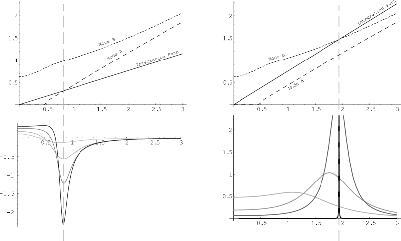
Figure 2: In the top plots we show the integration paths corresponding to (a) $v=0.5$ and (b) $v=0.99$ as solid lines along with the corresponding dispersion relations for the two infinite-$\xi$ unphysical modes (dashed and dotted lines labelled as “Mode A” and “Mode B”). In the bottom plots we show the corresponding value of the integrand of Eq. (20) evaluated along the integration paths shown in the top plots. We also plot the integrand of Eq. (20) for $\xi=\{1000,100,10\}$ as decreasingly lighter gray lines in the bottom plot. Note that in both (a) and (b) the integration paths in the top plots should be understood to terminate at $q=q^{*}$.

Let us discuss the case of $v=0.5$ first: as indicated by the vertical line in Fig. 2(a), the extremal contribution to the energy loss occurs when the integration path comes closest to the mode A. However, it turns out the contribution from this mode is negative, representing an inversion of the usual Landau-damping mechanism (we will discuss this issue later on). This situation is not limited to infinite anisotropies. In the bottom plot of Fig. 2(a) we show the integrand of Eq. (20) for $\xi=\{1000,100,10\}$ as decreasingly lighter gray lines. As we can see the effect remains but becomes less as the anisotropy parameter is decreased.

In Fig. 2(b) we show the same quantities but for $v=0.99$. As indicated by the vertical line in Fig. 2(b), the extremal contribution to the energy loss in this case occurs when the integration path comes closest to the mode B. However, in contrast, mode B contributions to the integrand are positive. Again, this behavior persists at finite $\xi$ as shown by the corresponding plots of the integrand of Eq. (20) for $\xi=\{1000,100,10\}$ in Fig. 2(b) (shown as increasingly lighter gray lines). However, the peak of the integrand for mode B contributions moves considerably more than the mode A contributions as $\xi$ is decreased.

As shown by the light gray lines in the lower plots of Fig. 2, the unphysical A and B modes seem to have the same qualitative effect on the energy loss at finite $\xi$ as they do in the limit of $\xi\rightarrow\infty$. However, since the modes move farther away from the physical region as $\xi$ is decreased, it is clear that their influence becomes smaller, as already argued in Ref. Romatschke:2004jh . Nevertheless, it is interesting to note that even for small values of $\xi$, mode A is capable of driving the soft energy loss contribution negative for small velocities $v$. Indeed, it turns out that in the limit $v\rightarrow 0$, one finds that the soft energy loss is purely negative (independent of the angle), as long as $\xi>0$.

This negative energy loss contribution is, however, not due to the fact that a particle with sub-thermal velocities should receive energy from the medium, since our approximation was based on the assumption of an infinitely heavy quark (see the discussion about limitations in the next section). Rather, since mode A is the analytic continuation of the plasma instability present on the physical sheet, we interpret the gain of energy as being intimately related to the presence of such instabilities. This is not a surprising finding given that if there are truly unstable modes in the system the energy for their growth must come from a mechanism which is also collective since it would be hard to imagine that a collisional mechanism could ever be fast enough.

The mode A contributions to the soft energy “loss” represent such a collective mechanism for the efficient transfer of energy from hard to soft scales. As we will show below the energy gain is focused in such a way that particles with small velocities are accelerated out-of-plane thereby reducing the anisotropy. In closing we note that for angles different than $\theta_{v}=0$, the connection between the modes on the neighboring unphysical sheets and the integrand of the energy loss remains but it is more difficult to disentangle since there is also an averaging over the azimuthal angle as well.

IV Heavy Quark Energy Loss

The collisional energy loss of a heavy quark in an anisotropic quark-gluon plasma to leading order in the coupling is given by adding the contributions Eq. (6) and Eq. (LABEL:myelosshard3)

$$\left(\frac{dW}{dx}\right)=\left(\frac{dW}{dx}\right)_{\rm soft}+\left(\frac{dW}{dx}\right)_{\rm hard}.$$ (21)

In all results presented below we will assume $N_{c}=3$ and $N_{f}=2$.

IV.1 Isotropic results

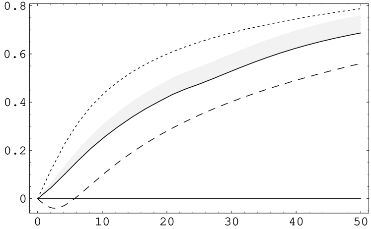
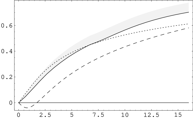
Figure 3: Isotropic energy loss of a bottom (a) and charm quark (b) as a function of momentum $p$ for $\alpha_{s}=0.3$. Shown are the respective results from Bjorken Bjorken:1982tu (dotted line) and Braaten and Thoma Braaten:1991we (dashed line) as well as the evaluation of Eq. (21) (full line) with a variation of $q^{*}$ (gray band).

In order to compare with existing calculations we first consider the isotropic limit ($\xi=0$). In this case the collisional energy loss is a function of the strong coupling $\alpha_{s}$, the particle velocity $v$, the temperature $T$, and the momentum separation scale $q^{*}$. The $q^{*}$ dependence of the result is found to become weak for small values of the coupling limit $\alpha_{s}$ (similar to what has been found in QED Romatschke:2003vc ), corresponding to the original result by Braaten and Thoma Braaten:1991we ; for larger values of the coupling one fixes $q^{*}=q^{\rm pms}$ using the principle of minimum sensitivity

$$\frac{d}{dq^{*}}\left.\left(\frac{dW}{dx}\right)\right|_{q^{*}=q^{*}_{\rm pms}}=0\,.$$ (22)

Note that in this case $-\left.\left(dW/dx\right)\right|_{q^{*}=q^{*}_{\rm pms}}$ always serves as a lower bound on the result for the energy loss. To get an estimate of how strongly the result depends on this special value of $q^{*}$, one can e.g. vary $q^{*}_{\rm pms}$ by a certain factor $c_{q^{*}}$ and evaluate the energy loss at $q^{*}_{\rm pms}c_{q^{*}}$ and $q^{*}_{\rm pms}/c_{q^{*}}$. This factor $c_{q^{*}}$ is in principle arbitrary; here we fix it to be $c_{q^{*}}=2$ to be consistent with what has been done in QED Romatschke:2003vc .

In Fig. 3 various results for the heavy quark energy loss in an isotropic quark-gluon plasma are compared: shown are the results from Bjorken Bjorken:1982tu , Braaten and Thoma Braaten:1991we , as well as Eq. (21) with $\xi=0$ at $q^{*}=q^{*}_{\rm pms}$ together with its variation using $c_{q^{*}}=2$. Both plots assume $\alpha_{s}=0.3$. Fig. 3(a) shows the energy loss of a bottom quark with mass $M_{Q}=5$ GeV while in Fig. 3(b) the energy loss of a charm quark with mass $M_{Q}=1.5$ GeV is plotted, both as a function of their momenta

$$p=\frac{vM_{Q}}{\sqrt{1-v^{2}}}\;.$$ (23)

In closing we would like to emphasize that our result is not only compatible with previous results on isotropic collisional energy loss but, in fact, represents the most complete calculation of this quantity to date. In contrast to the result of Bjorken Bjorken:1982tu it gives the correct leading-order result in the weak-coupling limit as does the result of Braaten and Thoma Braaten:1991we ; however, as noted before, at realistic values of the coupling and small momentum the Braaten and Thoma result breaks down completely. In the isotropic case our result is positive definite as it should be for an infinitely massive quark. In addition the use of a principle-of-minimal sensitivity to fix the scale gives the added benefit of being able to place theoretical error bars on the results obtained.

IV.2 Limitations

Since Eq. (21) has been derived assuming an infinitely heavy quark we have to determine what will happen if we instead have only a heavy quark like a charm or bottom quark. The chief consequence is that for sub-thermal velocities defined by $v\,\raisebox{-2.84526pt}{$\stackrel{{\scriptstyle<}}{{\sim}}$}\,\sqrt{T/M_{Q}}$ the approximation breaks down because quarks with those velocities will gain energy from collisions with other particles in the heat bath instead of losing energy. Below this threshold the energy loss would then turn into energy gain. A semi-quantitative estimate of the velocity where the isotropic energy loss becomes negative has been performed in Ref. Braaten:1991we by repeating the above calculation in the limit $v\rightarrow 0$ and for weak couplings, finding $v\,\raisebox{-2.84526pt}{$\stackrel{{\scriptstyle<}}{{\sim}}$}\,\sqrt{3T/M_{Q}}$. Using $T=250$ MeV and the masses above, this velocity corresponds to $p=2.1$ GeV and $p=1.5$ GeV for bottom and charm, respectively. Similarly, Eq. (21) also breaks down for ultrarelativistic energies $E\gg M_{Q}^{2}/T$, with the cross-over energy having been determined to be $E_{\rm cross}\simeq 1.8\,M_{Q}^{2}/T$ (corresponding to $v>0.995$ for both charm and bottom quarks).

In contrast the Braaten and Thoma results shown in Fig. 3 turn negative at a momentum of $p\simeq 5.7$ GeV for the bottom and $p\simeq 1.71$ GeV for the charm quark. This behavior is not due to the physical reason discussed above but rather due to a failure of the extrapolation from the weak-coupling limit to realistic couplings Braaten:1991we . For the unexpanded isotropic result Eq. (21), this unphysical behavior does not occur (it is always positive) and one can therefore expect it to be valid for velocities down to the original estimate $v\sim\sqrt{3T/M_{Q}}$. In anisotropic systems, however, this rule of thumb no longer applies and negative energy loss does not require the heavy quark to have sub-thermal velocity. Instead, as already noted by Lifshitz and Pitaevskii Pitae:1981 , this type of energy gain is connected to the instabilities of the system, as we have argued in the previous section.

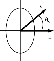
Figure 4: Sketch of the vectors relevant to the directional dependence of the energy loss: $\bf\hat{n}$ is the direction of the anisotropy, ${\bf v}$ the velocity of the quark, and $\theta_{v}$ the angle between these. We have also plotted an isocontour of a $\xi>0$ distribution function for comparison.

Before moving on to the anisotropic results let us briefly comment on the variation estimate based on setting $c_{q^{*}}=2$: while for QED this represents a very conservative choice on the variations since $m_{D}\ll q^{*}_{pms}\ll 2\pi T$, in QCD one encounters situations with $q^{*}_{pms}>2\pi T$ or $q^{*}_{pms}<m_{D}$ for realistic couplings like $\alpha_{s}=0.3$ since $m_{D}$ and $2\pi T$ are no longer well separated. Strictly speaking, the method we are using is breaking down at realistic couplings; nevertheless, by using variations with $c_{q^{*}}=2$ we can hope to obtain reasonable estimates of the leading-order results when the difference between these variations is not too large. Finally, it should be noted that no estimate of the next-to-leading order (NLO) radiative corrections to the energy loss has been made here. Therefore, it should be kept in mind that for QCD with large realistic coupling the inclusion of these NLO corrections might give energy loss results that are not covered by the variations of $q^{*}$ in the leading-order result, so these variations should be interpreted with care.

IV.3 Anisotropic results

For an anisotropic system with (gluon and quark) anisotropy strength $\xi$, the collisional energy loss result Eq. (21) depends on $q^{*}$, $T$, and $v$ as was the case for the isotropic energy loss, but in general also on the angle of the particle propagation with respect to the anisotropy vector $\cos\theta_{v}={\bf\hat{v}\cdot\hat{n}}$ (sketched in Fig. 4). As in the isotropic case the total result is obtained by combining the soft and hard contributions to the energy loss. In Figs. 6-8 we plot the hard and soft contributions to the energy loss together with their sum as a function of $q^{*}/T$ for $\alpha_{s}=\{1\times 10^{-4},1\times 10^{-3},0.01,0.3\}$ corresponding to $m_{D}/T=\{0.041,0.13,0.41,2.2\}$. As can be seen from these Figures the soft contribution (dashed line) is always negative over some range of $q^{*}/T$. For small couplings (see Fig. 6) this negative contribution is in a region where there is always a larger positive hard contribution. However, as the coupling constant is increased we see that the range of $q^{*}/T$ over which the soft contribution is negative moves to higher scales and eventually dominates the sum of the soft and hard contributions over a range of $q^{*}$ (see Fig. 8).

Figure 5: Anisotropic energy loss for $\xi=10.0$, $\alpha_{s}=1\times 10^{-4}$, $v=0.1$, and $\theta_{v}=0$ as a function of $q^{*}$. Dotted, dashed, and solid lines are the hard contribution, the soft contribution, and their sum, respectively.

Figure 6: Anisotropic energy loss for $\xi=10.0$, $\alpha_{s}=1\times 10^{-3}$, $v=0.1$, and $\theta_{v}=0$ as a function of $q^{*}$. Dotted, dashed, and solid lines are the hard contribution, the soft contribution, and their sum, respectively.

Figure 7: Anisotropic energy loss for $\xi=10.0$, $\alpha_{s}=0.01$, $v=0.1$, and $\theta_{v}=0$ as a function of $q^{*}$. Dotted, dashed, and solid lines are the hard contribution, the soft contribution, and their sum, respectively.

Figure 8: Anisotropic energy loss for $\xi=10.0$, $\alpha_{s}=0.3$, $v=0.1$, and $\theta_{v}=0$ as a function of $q^{*}$. Dotted, dashed, and solid lines are the hard contribution, the soft contribution, and their sum, respectively.

For all $\xi$ we find that the soft energy loss has a minimum at some value of $q^{*}$. For small $v$ this minimum can even be negative as explicitly demonstrated in Figs. 8 and 8. Considering again $\theta_{v}=0$ for guidance we notice that the limits on the integration in Eq. (20) correspond to a triangular region defined by $0\leq\omega\leq qv$ and $q\leq q^{*}$. From this we observe that when $q^{*}$ is small we only receive contributions from mode A which are predominantly negative. As $q^{*}$ is increased, however, we start to receive large positive contributions from mode B. Defining $q^{*}_{c}$ as the point where the upper boundary defined by $\omega=qv$ hits mode B we obtain $q^{*}_{c}=\omega_{B}/v$. In order to estimate the value of $q_{c}^{*}$ we again consider the limit $\xi\rightarrow\infty$. The dispersion relation for mode B at $\theta_{q}=0$ and $\xi=\infty$ is known and is $q$-independent Romatschke:2004jh

$$\omega_{B}^{2}=\frac{\pi}{4}m_{D}^{2}\,.$$ (24)

Using this we obtain

$$q_{c}^{*}=\sqrt{\frac{\pi}{4}}\frac{m_{D}}{v}\,.$$ (25)

For larger values of $q^{*}$, the negative contributions also become larger, but there is also now a strongly positive contribution from mode B (even for nonzero $\theta_{q}$), so that the overall result turns out to be more positive than at $q^{*}_{c}$. On the other hand, for $q^{*}<q^{*}_{c}$, the main negative contributions become smaller since the “region” they are integrated over has shrunk. Therefore, the minimum of the soft contribution to the energy loss for $\xi\rightarrow\infty$ at $\theta_{v}=0$ is obtained around $q^{*}_{c}$. This can be used as a rough guideline for the location of this minimum also for large but finite $\xi$, however, as $\xi$ is decreased $q_{c}^{*}$ moves to lower values of $q^{*}$ and the depth of the minimum decreases.

Returning to the results for the total anisotropic energy loss (hard plus soft) we again fix the scale $q^{*}$ by the application of the principle of minimal sensitivity (22) as in the isotropic case; however, in order to keep the figures presented as understandable as possible we do not show the corresponding variation of $q^{*}$ by $c_{q^{*}}=2$. Instead we note that the sensitivity of the anisotropic results to this scale is similar to the isotropic variation indicated by the gray band in Fig. 3, however, there is an increase in the magnitude of the variation as $\xi$ is increased. For example, at $\xi=\infty$ the corresponding variation is approximately three times the corresponding isotropic variation.

Figure 9: Anisotropic energy loss for $\xi=1.0$, $\alpha_{s}=0.3$ and $\theta_{v}=0$ (dotted line) compared to $\theta=\pi/2$ (dashed line) as a function of velocity (normalized to the isotropic result, full line).

Figure 10: Anisotropic energy loss for a bottom quark for $\xi=1.0$, $\alpha_{s}=0.3$ and $\theta_{v}=0$ (dotted line), $\theta_{v}=\pi/2$ (dashed line) compared to the isotropic result (full line).

In Fig. 10 we show the energy loss Eq. (21) for a heavy quark propagating parallel to the anisotropy direction ($\theta_{v}=0$) and perpendicular to the anisotropy direction ($\theta_{v}=\pi/2$) as a function of the heavy quark velocity $v$ with $\alpha_{s}=0.3$ and $\xi=1$. The results shown are normalized to the isotropic energy loss. As can be seen from this Figure for small velocities the energy loss is larger at $\theta_{v}=\pi/2$ while for large velocities it is larger at $\theta_{v}=0$. This is similar to the behavior found for a QED plasma Romatschke:2003vc .

In Fig. 10 we show the corresponding energy loss for a bottom quark with $M_{Q}=5$ GeV using the relation between velocity and momentum given in Eq. (23). We have not normalized this result as before but instead include the corresponding isotropic result as a solid line for comparison. As can be seen from this Figure for $\xi=1$ and $\alpha_{s}=0.3$ the energy loss of a bottom quark with $\theta_{v}=\pi/2$ is almost indistinguishable from the isotropic result while the energy loss with $\theta_{v}=0$ is larger than the isotropic result for $p\,\raisebox{-2.84526pt}{$\stackrel{{\scriptstyle>}}{{\sim}}$}\,6$ GeV. For example, for a 20 GeV bottom quark we find that the energy loss at $\theta_{v}=0$ is approximately 10% higher than the isotropic result.

It should be noted that for very small velocities, the energy loss for the angle $\theta_{v}=0$ becomes negative because of the presence of modes on the unphysical sheet as discussed in Sec. III. However, for $\xi=1.0$ this occurs at very small velocities where the heavy quark approximation used is invalid in any case so that within the valid range of velocities ($v\geq 0.39$ and $v\geq 0.71$ for bottom and charm quarks, respectively) the energy loss is always positive.

Figure 11: Anisotropic energy loss for $\xi=10.0$, $\alpha_{s}=0.3$ and $\theta_{v}=0$ (dotted line) compared to $\theta=\pi/2$ (dashed line) as a function of velocity (normalized to the isotropic result, full line).

Figure 12: Anisotropic energy loss for a bottom quark for $\xi=10.0$, $\alpha_{s}=0.3$ and $\theta_{v}=0$ (dotted line), $\theta_{v}=\pi/2$ (dashed line) compared to the isotropic result (full line).

In Figs. 12 and 12 we present the same plots but for $\xi=10$. As can be seen from Fig. 12 for small velocities the energy loss is larger at $\theta_{v}=\pi/2$ while for large velocities it is larger at $\theta_{v}=0$ similar to the situation at $\xi=1$. From Fig. 12 we see that the bottom quark energy loss at $\theta_{v}=\pi/2$ is less than the isotropic result while the energy loss at $\theta_{v}=0$ is larger than the isotropic result for $p\,\raisebox{-2.84526pt}{$\stackrel{{\scriptstyle>}}{{\sim}}$}\,8$ GeV. For example, for a 20 GeV bottom quark we find that the energy loss for $\theta_{v}=\pi/2$ is approximately 10% lower than the isotropic result and for $\theta_{v}=0$ the energy loss is approximately 20% higher than the isotropic result. Again for velocities less than $v\sim 0.4$ the energy loss at $\theta_{v}=0$ becomes negative; however, now the velocity where it becomes negative is on the border of the applicability of the heavy quark approximation for a bottom quark given in the previous paragraph. One is therefore lead to wonder what happens if we continue to increase the anisotropy.

Figure 13: Anisotropic energy loss for $\xi\rightarrow\infty$, $\alpha_{s}=0.3$ and $\theta_{v}=0$ (dotted line) compared to $\theta_{v}=\pi/2$ (dashed line) as a function of velocity (normalized to the isotropic result, full line).

Figure 14: Anisotropic energy loss for a bottom quark for $\xi\rightarrow\infty$, $\alpha_{s}=0.3$ and $\theta_{v}=0$ (dotted line), $\theta_{v}=\pi/2$ (dashed line) compared to the isotropic result (full line).

IV.4 Infinite anisotropy limit

As Figs. 10 and 12 demonstrate, as the anisotropy strength $\xi$ is increased the directional dependence of the heavy quark energy loss increases. Additionally we found that the velocity at which the energy loss becomes negative increases as $\xi$ is increased. It would be very instructive to then consider the limit of $\xi\rightarrow\infty$ to see the limiting behavior of the energy loss.

In Figs. 14 and 14 we present the same plots but for $\xi=\infty$. As can be seen from Fig. 14 for small velocities the energy loss is larger at $\theta_{v}=\pi/2$ while for large velocities it is larger at $\theta_{v}=0$ similar to what we found at finite $\xi$. From Fig. 14 we see that the energy loss of a bottom quark with $\theta_{v}=\pi/2$ is less than the isotropic result while the energy loss of a bottom quark with $\theta_{v}=0$ is larger than the isotropic result for $p\,\raisebox{-2.84526pt}{$\stackrel{{\scriptstyle>}}{{\sim}}$}\,10$ GeV; however, the results are not dramatically different than those obtained at $\xi=10$. However, the velocity where the energy loss becomes negative, $v\sim 0.65$, is well within the range of applicability of the heavy quark approximation for a bottom quark ($v\geq 0.39$). We are therefore led to the conclusion that for very strong anisotropies heavy quarks with small velocities will experience an energy gain rather than an energy loss. Additionally we see that the energy loss is more negative at $\theta_{v}=0$ than any other angle of propagation. This means particles moving along the anisotropy direction experience the most energy gain. This is a rather surprising result but its origin can be traced to the presence of modes on the unphysical sheet as discussed in Sec. III. These modes therefore represent a qualitative change to the physics in highly anisotropic plasmas.

V Conclusions

In this paper we have calculated the complete leading-order collisional energy loss of a heavy quark propagating through an anisotropic quark-gluon plasma. The results were presented as a function of the heavy quark velocity and propagation angle. We presented a discussion concerning the kinematical range over which the results obtained here apply when the quark mass is large but not infinite and we then explicitly applied the results to the energy loss of a bottom quark in an anisotropic setting. It was shown that for anisotropic systems the collisional energy loss has an angular dependence which increases as the coupling and/or anisotropy is increased as expected on intuitive grounds. Quantitatively, for $\alpha_{s}=0.3$ and a 20 GeV bottom quark we found that the deviations from the isotropic result were on the order of 10% for $\xi=1$ and of the order of 20% for $\xi\geq 10$. When translated into the difference between longitudinal and transverse energy loss this results in a 10% difference at $\xi=1$, a 30% difference at $\xi=10$, and a 50% difference at $\xi=\infty$.

More importantly, however, we found that for small velocities the sign of the energy loss becomes negative representing energy gain instead of loss whenever $\xi>0$. In the isotropic limit and assuming an infinitely heavy quark it can be shown that the energy loss is positive definite and our results confirm this expectation for isotropic systems in contrast to the earlier calculation of Braaten and Thoma. In the anisotropic case, however, there is no guarantee that the energy loss will be a positive quantity. We have shown here that the negative contributions to the energy loss come from singularities on the neighboring unphysical sheets which are not present in the isotropic case Romatschke:2004jh . For small anisotropies the velocities at which the energy loss becomes negative are lower than the thermal bound set by $v\sim\sqrt{3T/m}$. For large anisotropies the velocities at which the energy loss becomes negative for a bottom quark are above the thermal lower bound and are therefore within the range of applicability of the infinite quark mass limit considered here.

The results we have presented for the heavy quark energy loss should be compared with the expected momentum-space anisotropy generated during the early stages of RHIC and LHC heavy-ion collisions. At the earliest times that a particle description is appropriate the relevant scales are $p_{T}\sim Q_{s}$ where $Q_{s}$ is of order 1 GeV at RHIC and 2-3 GeV at LHC energies and $p_{z}\sim 1/\tau$ where $\tau$ is the time at which the hard gluon occupation number drops below 1. In order to estimate $\tau$ we follow the logic used in the bottom-up thermalization scenario BMSS:2001 giving parametrically $Q_{s}\tau\sim\alpha_{s}^{-3/2}$. We therefore estimate that parametrically $p_{z}\sim\alpha_{s}^{3/2}Q_{s}$ and as a result $\xi\sim\alpha_{s}^{-3/2}$. We therefore see that in the weak-coupling limit large anisotropies can be generated if the bottom-up scenario is true. Using a realistic coupling of $\alpha_{s}\sim 0.3$ gives $\xi\sim 6$ but this estimate could change dramatically depending on the specific coefficients omitted in our parametric estimates. Additionally the time estimate $Q_{s}\tau\sim\alpha_{s}^{-3/2}$ is based on an implicit assumption of isotropy and collisional broadening and must be revisited in the context of an anisotropic quark-gluon plasma. Also in terms of producing phenomenologically relevant predictions it should be mentioned that since there are unstable modes present in the system, whatever value of $\xi$ one starts with, it is expected to go to zero very rapidly. In order to predict the total effect on observables we would need to fold together the results obtained here with the time evolution of $\xi$ which is not currently available.

It should be mentioned that thermal effects are only expected to make the energy loss more negative at small velocities; however, it would be nice to have an explicit calculation of the anisotropic energy loss in the limit $v\rightarrow 0$ with the infinite-mass assumption relaxed. Additionally, a refinement of the calculation involving different momentum-space anisotropies for the quark and gluon distribution functions was suggested. Another area for improvement is that this work ignores next-to-leading order radiative energy loss. In isotropic systems it has been shown that the radiative energy loss of a heavy quark is larger than the collisional energy loss and thus cannot be ignored. As illustrated by this work, however, a calculation of the radiative energy loss for an anisotropic system would be considerably more involved than the equivalent calculation in an isotropic one. Nevertheless, it seems necessary in order to truly understand heavy quark energy loss in an anisotropic plasma.

References

- (1) K. Adcox et al. (PHENIX Collaboration), Phys. Rev. Lett. 88, 192302 (2002).
- (2) J.L. Nagle et al. (PHENIX Collaboration), arXiv:nucl-ex/0209015.
- (3) E. Braaten and M. H. Thoma, Phys. Rev. D44, 1298 (1991).
- (4) E. Braaten and M. H. Thoma, Phys. Rev. D44, 2625 (1991).
- (5) P. Romatschke and M. Strickland, Phys. Rev. D69, 065005 (2004).
- (6) R. Baier, D. Schiff, and B. G. Zakharov, Ann. Rev. Nucl. Part. Sci. 50, 37 (2000).
- (7) A. Accardi et al., arXiv:hep-ph/0310274 (2003).
- (8) E.S. Weibel, Phys. Rev. Lett. 2, 83 (1959).
- (9) St. Mrówczyński, Phys. Lett. B314, 118 (1993).
- (10) St. Mrówczyński, Phys. Rev. C49, 2191 (1994).
- (11) St. Mrówczyński, Phys. Lett. B393, 26 (1997).
- (12) J. Randrup and St. Mrówczyński, Phys. Rev. C68, 034909 (2003).
- (13) P. Romatschke and M. Strickland, Phys. Rev. D68, 036004 (2003).
- (14) P. Arnold, J. Lenaghan, and G. D. Moore, JHEP 08, 002 (2003).
- (15) St. Mrówczyński, A. Rebhan, M. Strickland, Phys.Rev. D70, 025004 (2004).
- (16) P. Romatschke, “Quasiparticle description of the hot and dense quark gluon plasma,” PhD Dissertation, arXiv:hep-ph/0312152 (2003).
- (17) P. Romatschke and M. Strickland, arXiv:hep-ph/0406188 (2004).
- (18) P. Arnold and J. Lenaghan, arXiv:hep-ph/0408052 (2004).
- (19) M. H. Thoma and M. Gyulassy, Nucl. Phys. B351, 491 (1991).
- (20) J. D. Bjorken, FERMILAB-PUB-82-059-THY (1982).
- (21) E.M. Lifshitz and L.P. Pitaevskii, Physical Kinetics, Pergamon Press, Oxford, §30 (1981).
- (22) R. Baier, A.H. Mueller, D. Schiff, and D.T. Son, Phys. Lett. B 502, 51 (2001).