Shape Function Effects in $B\to X_{c}\ell\bar{\nu}_{\ell}$

Abstract

Owing to the fact that $m_{c}^{2}\sim m_{b}\Lambda_{\text{QCD}}$, the endpoint region of the charged lepton energy spectrum in the inclusive decay $B\to X_{c}\ell\bar{\nu}_{\ell}$ is affected by the Fermi motion of the initial-state $b$ quark bound in the $B$ meson. This effect is described in QCD by shape functions. Including the mass of the final-state quark, we find that a different set of operators as employed in Ref. Bauer:2002yu is needed for a consistent matching, when incorporating the subleading contributions in $B\to X_{q}\ell\bar{\nu}_{\ell}$ for both $q=u$ and $q=c$. In addition, we modify the usual twist expansion in such a way that it yields a description of the lepton energy spectrum which is not just valid in the endpoint region, but over the entire phase space.

I Introduction

The theoretical machinery for the determination of $\lvert V_{cb}\rvert$ from semileptonic $B$-meson decays has reached a mature state over the last years. With the very precise data on the exclusive $B\to D^{(*)}\ell\bar{\nu}_{\ell}$ channels as well as on the inclusive decays $B\to X_{c}\ell\bar{\nu}_{\ell}$ from the $B$-meson factories the theoretical description has been improved so much that currently relative theoretical uncertainties for $\lvert V_{cb}\rvert$ of less than 2% are quoted Benson:2003kp ; Bauer:2004ve , yielding a total uncertainty of about 2% Aubert:2004aw .

The nonperturbative corrections to the inclusive decays are parametrically of order $1/m_{b}^{2}$ and hence are expected to be smaller than in the exclusive channels, where the corrections are of order $1/m_{c}^{2}$. However, the inclusive rate depends on the $b$-quark mass $m_{b}$, which needs to be determined in a suitable scheme as precisely as possible.

In addition, also the parameters of the heavy quark expansion are needed, such as $\lambda_{1}$ and $\lambda_{2}$ at order $1/m_{b}^{2}$ and the corresponding parameters appearing at higher orders. These parameters are obtained experimentally by taking moments of the various inclusive distributions (such as lepton energy spectra or hadronic invariant mass distributions), but the higher moments become more and more sensitive to higher-order corrections in $1/m_{b}$, since the leading contribution to the $n$th moment is roughly of the order $1/m_{b}^{n}$.

When determining the heavy quark parameters from the lepton energy spectrum, the higher moments become sensitive to the endpoint region of the spectrum. Using the $1/m_{b}$ expansion the leading term is the partonic rate and still a smooth function, but already the first non-vanishing nonperturbative contribution exhibits an irregular behavior which is unphysical. The situation is in fact very similar to the one in $b\to u$ transitions, where it is known that these singular contributions can be resummed into a shape function. For heavy to light decays, such as the decays $b\to u\ell\bar{\nu}_{\ell}$ and $b\to s\gamma$, the twist expansion, that is, the resummation of nonperturbative contributions, has been performed to the subleading level in the $1/m_{b}$ expansion BLM1 ; Bauer:2002yu ; BLM21 ; Burrell:2003cf .

It has already been noticed some time ago Mannel:1994pm that the light-cone distribution of the $B$ meson also has a significant effect on the endpoint region of the lepton energy spectrum in $B\to X_{c}\ell\bar{\nu}_{\ell}$. This is due to the fact that numerically $m_{c}^{2}\sim m_{b}\Lambda_{\text{QCD}}$. The charm quark mass thus has to be counted as $\sqrt{m_{b}\Lambda_{\text{QCD}}}$ when performing the power counting. The endpoint region is known to be determined by the light-cone distribution of the initial state and has the width $\sqrt{m_{b}\Lambda_{\text{QCD}}}$, which happens to be of the same order as $m_{c}$. Therefore, it is useful to consider the effects of the light-cone distribution of the $B$ meson also in $B\to X_{c}\ell\bar{\nu}_{\ell}$.

In the present paper we perform this analysis and compare with the standard expansion. As a by-product, we suggest a modified twist expansion which can be applied over the full phase space, incorporating the twist expansion in the endpoint region as well as the usual local expansion in the rest of phase space.

Furthermore, performing the limit $m_{c}\to 0$ we discover an inconsistency in comparison with previous work Bauer:2002yu . It turns out that at subleading order additional operators are needed which are formally of leading order, but have coefficients of subleading order. Expanding into the usual local expansion we obtain the correct result for the terms of order $1/m_{b}^{3}$, indicating that our result is consistent. As a consequence, compared to Ref. Bauer:2002yu additional nonperturbative input in the form of new shape functions appears.

I.1 Inclusive Decay Rate

Neglecting the masses of the leptons the energy spectrum of the charged lepton in the $B$ rest frame is given via the optical theorem by

$$\frac{\mathrm{d}\Gamma_{q}}{\mathrm{d}y}=4\Gamma_{0}y^{2}\theta(y)\langle T_{q}\rangle_{\!B},$$ (1)

where $y=2E_{\ell}/m_{b}$ denotes the rescaled lepton energy,

$$\Gamma_{0}=\frac{G_{F}^{2}\lvert V_{qb}\rvert^{2}m_{b}^{5}}{192\pi^{3}},$$

and $q$ stands for either $u$ or $c$. The “$B$ expectation value” is defined as $\langle\mathcal{O}\rangle_{\!B}=\langle B\lvert\mathcal{O}\rvert B\rangle/2m_{B}$, where the QCD states are normalized to $2m_{B}$. The operator $T_{q}$ has the form

$$T_{q}=\frac{48\pi^{2}}{m_{b}^{3}y}\mathrm{Im}\,\frac{\mathrm{i}}{\pi}\sum_{s_{\ell}}\int\mathrm{d}^{4}x\,e^{-\mathrm{i}p_{\ell}\cdot x}T\bigl{[}W_{q}^{\dagger}(x)W_{q}(0)\bigr{]},$$ (2)

where $s_{\ell}$ and $p_{\ell}$ are the lepton spin and momentum. The effective weak current is

$$W_{q}=(\bar{q}\gamma_{\alpha}P_{L}b)(\bar{u}_{\ell}\gamma^{\alpha}P_{L}\nu_{\ell})=(\bar{q}\gamma_{\alpha}P_{L}\nu_{\ell})(\bar{u}_{\ell}\gamma^{\alpha}P_{L}b),$$

with $P_{L}=(1-\gamma_{5})/2$ and $u_{\ell}$ denoting the lepton spinor. Plugging this into Eq. (2) yields

$$T_{q} =\frac{48\pi^{2}}{m_{b}^{3}y}\biggl{(}-\frac{1}{\pi}\mathrm{Im}\,\bar{b}L_{\alpha\beta}b\Pi_{q}^{\alpha\beta}\biggr{)}\quad\text{with}$$ (3a)

$$L_{\alpha\beta} =\gamma_{\alpha}{p\mspace{-7.5mu}/\mspace{-1.5mu}}_{\ell}\gamma_{\beta}P_{L},$$ (3b)

$$\Pi_{q}^{\alpha\beta} =-\mathrm{i}\!\int\mathrm{d}^{4}xe^{\mathrm{i}(p_{b}-p_{\ell})\cdot x}T\bigl{[}(\bar{\nu}_{\ell}\gamma^{\alpha}P_{L}q)(x)(\bar{q}\gamma^{\beta}P_{L}\nu_{\ell})(0)\bigr{]}.$$ (3c)

Here, $L_{\alpha\beta}$ is the leptonic tensor and $\Pi_{q}^{\alpha\beta}$ represents the inclusive $q$-quark-neutrino loop with the momentum transfer $p_{b}-p_{\ell}$. The $b$-quark momentum $p_{b}$ contains a large part $m_{b}v$, where $v$ is the velocity of the $B$ meson. As usual, assuming that $Q=m_{b}v-p_{\ell}$ sets a perturbative scale, large compared to $k=p_{b}-m_{b}v\sim\mathcal{O}(\Lambda_{\text{QCD}})$, we may perform an OPE of the transition operator $T_{q}$ in powers of $\Lambda\equiv\Lambda_{\text{QCD}}/m_{b}$ ManoharWise ; Bigiinclusive1 ; Mannelinc .

I.2 Light-Cone Vectors and Power Counting

Using appropriate powers of $m_{b}$ we may work with dimensionless variables, which are denoted by a hat, for example $\hat{Q}=Q/m_{b}=v-\hat{p}_{\ell}$. We also define $\Delta=1-y$ and $\rho=m_{c}^{2}/m_{b}^{2}$.

As already noted, the $c$-quark mass satisfies $m_{c}^{2}\sim m_{b}\Lambda_{\text{QCD}}$ and thus $\rho\sim\mathcal{O}(\Lambda)$. The kinematic endpoint in the local OPE is given by $\Delta=\rho$, the partonic endpoint. The endpoint region of the lepton energy spectrum is defined by $\Delta\sim\mathcal{O}(\Lambda)$, and it is well known ManoharWise that in this region the local OPE breaks down. However, it has been shown that one may still perform a light-cone or twist expansion NeubertShape ; NeubertShape1 ; BigiMotion .

To set up the light-cone expansion we use the velocity $v$ and the lepton momentum $p_{\ell}$ to define a basis of two light-cone vectors,

$$v=\frac{1}{2}(n+\bar{n}),\quad p_{\ell}=E_{\ell}\bar{n}=\frac{m_{b}}{2}y\bar{n},$$ (4a)

satisfying $$n^{2}=\bar{n}^{2}=0 n\cdot\bar{n}=2$$ and . The metric is decomposed accordingly

$$\eta^{\mu\nu}=\frac{1}{2}n^{\mu}\bar{n}^{\nu}+\frac{1}{2}\bar{n}^{\mu}n^{\nu}+\eta_{\perp}^{\mu\nu},$$ (4b)

and a generic four-momentum $$p$$ can be written as

$$p^{\mu}=\frac{1}{2}p_{-}n^{\mu}+\frac{1}{2}p_{+}\bar{n}^{\mu}+p_{\perp}^{\mu},$$ (4c)

where we defined

$$p_{+}=n\cdot p,\quad p_{-}=\bar{n}\cdot p,\quad p_{\perp}^{\mu}=\eta_{\perp}^{\mu\nu}p_{\nu}.$$ (4d)

The power counting

$$\hat{Q}_{-}=1,\quad\hat{Q}_{+}=\Delta\sim\mathcal{O}(\Lambda),\quad\rho\sim\mathcal{O}(\Lambda),\quad\hat{k}\sim\mathcal{O}(\Lambda),$$ (5)

yields the standard twist expansion by expanding in powers of $\Lambda$, taking also into account that $\rho\sim\mathcal{O}(\Lambda)$.

Note that this power counting becomes wrong for small lepton energies, since $\Delta$ becomes of $\mathcal{O}(1)$. In this case the spectrum is described by the usual local OPE. However, as we shall discuss below, with a slight modification of the twist expansion it is possible to describe the spectrum also for small lepton energies.

The relevant kinematic variable in the OPE is $\hat{p}=\hat{p}_{b}-\hat{p}_{\ell}=\hat{Q}+\hat{k}$, the light-cone components of which are

$$\hat{p}_{+}=\Delta+\hat{k}_{+},\quad\hat{p}_{-}=1+\hat{k}_{-},\quad\hat{p}_{\perp}=\hat{k}_{\perp}.$$ (6)

Obviously all $\hat{k}_{+}$ dependence occurs in the combination $\Delta_{+}=\Delta+\hat{k}_{+}$. In the local OPE the complete $\hat{k}$ dependence is expanded. In particular, this produces terms of the form $\hat{k}_{+}/\Delta$, which become large, of $\mathcal{O}(1)$, near the endpoint. The twist expansion avoids these terms, since only the $\hat{k}_{-}$ and $\hat{k}_{\perp}$ dependences are expanded.

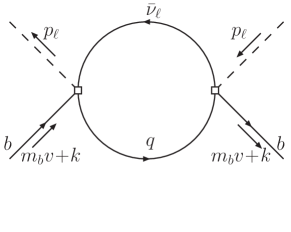
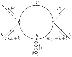
Figure 1: Feynman diagrams for the zero- and one-gluon matrix elements (to leading order in $\alpha_{s}$).

Alternatively to Eq. (5), we may as well treat the complete dependence on $\Delta_{+}$ (and $\rho$) exactly. That is, we use the power counting

$$\hat{k}_{-}\sim\mathcal{O}(\Lambda),\quad\hat{k}_{\perp}\sim\mathcal{O}(\Lambda),$$ (7)

and only expand in powers of $\hat{k}_{-}$ and $\hat{k}_{\perp}$ from the very beginning. The order in $\Lambda$ of a twist term given by Eq. (7) corresponds to the order of the first local term it contains, once the usual local OPE is performed. Eq. (7) defines what we call the modified twist expansion and holds for large and small lepton energies. Our results will therefore be valid over the whole lepton energy spectrum, providing a correct interpolation between the usual twist and local expansions.

Our modified expansion is a direct extension of the usual twist expansion. The latter does not expand $\Delta_{+}=\Delta+\hat{k}_{+}$ because both $\Delta$ and $\hat{k}_{+}$ are considered $\mathcal{O}(\Lambda)$. Once part of the $\hat{k}_{+}$ dependence is left unexpanded, it is consistent to keep the complete $\hat{k}_{+}$ dependence unexpanded, as it just means to keep correct small terms, which can now be treated exactly. This is similar to the local expansion, where $\rho=m_{c}^{2}/m_{b}^{2}$, although being numerically small, is always treated exactly, because it can be treated exactly. Once we exclude $\hat{k}_{+}$ from the power counting and treat it exactly, there is no need to count $\Delta$ as $\mathcal{O}(\Lambda)$ anymore. Thus we can treat it exactly much like $\rho$. This in turn extends the validity of our expansion down to low lepton energies (where numerically $\Delta$ is of order one which caused the breakdown of the usual twist expansion).

In other words, starting from the full expression (including all $\hat{k}$-components) both expansions expand the $\hat{k}_{-}$ and $\hat{k}_{\perp}$ components. This is where we stop, while the usual expansion additionally neglects terms of second and higher twist order caused by $\Delta_{+}$, e.g., terms like $\Delta_{+}^{2}$. We keep all those “kinematic” twist terms, because they are of $\mathcal{O}(1)$ for low lepton energies. Note that we do not claim to include all second-order twist contributions, i.e., our spectrum is only correct to $\mathcal{O}(\Lambda)$ in the endpoint region, but it is correct to $\mathcal{O}(\Lambda^{2})$ for low lepton energies.

Therefore, the difference to the usual twist expansion, defined by Eq. (5), is that the modified expansion automatically keeps all twist contributions that in the usual power counting are of higher order only because of additional factors of $\Delta_{+}$ or $\rho$. These contributions are purely kinematic and do not require additional operators in the twist expansion, but appear only as higher-order terms in the OPE coefficients. Taking them into account yields a consistent result valid over the full region of lepton energies.

II Operator Product Expansion

To keep things simple and to exhibit the structure of the OPE we will perform it in terms of QCD light-cone operators. Schematically, it has the form

$$T_{q}=\int\mathrm{d}\omega\sum_{n}C^{(n)}(\omega)\mathcal{O}_{n}(\omega).$$ (8)

In a second step the $B$ expectation values of the $\mathcal{O}_{n}(\omega)$ are parametrized in terms of shape functions.

We expand to $\mathcal{O}(\Lambda^{2})$ as defined by Eq. (7). With respect to the usual twist power counting this includes all contributions of leading and subleading twist, as well as some of second and even third order. In other words, we obtain the full coefficients of all operators with up to two covariant derivatives, which in particular retains all local terms up to local $\mathcal{O}(\Lambda^{2})$. To do so, we need to evaluate the zero- and one-gluon matrix elements of $T_{q}$, depicted in Fig. 1, which we do to leading order in $\alpha_{s}$.

II.1 Leading Twist

We first consider the case $q=c$ and later take the limit $m_{c}\to 0$. The zero-gluon matrix element of $T_{c}$ yields the well-known result

$$\langle b\lvert T_{c}\rvert b\rangle=\theta(\hat{p}^{2}-\rho)\Bigl{(}1-\frac{\rho}{\hat{p}^{2}}\Bigr{)}^{2}\\ \times\biggl{[}\Bigl{(}1+2\frac{\rho}{\hat{p}^{2}}\Bigr{)}3\eta_{(\mu\nu}\bar{n}_{\alpha)}\hat{p}^{\mu}\hat{p}^{\nu}-3\rho\bar{n}_{\alpha}\biggr{]}\bar{u}_{b}\gamma^{\alpha}P_{L}u_{b}.$$ (9)

Indices in round brackets are completely symmetrized,

$$\eta_{(\mu\nu}\bar{n}_{\alpha)}=\frac{1}{3}(\eta_{\mu\nu}\bar{n}_{\alpha}+\eta_{\mu\alpha}\bar{n}_{\nu}+\eta_{\alpha\nu}\bar{n}_{\mu}).$$

Extracting the terms of $\mathcal{O}(1)$,

$$\langle b\lvert T_{c}\rvert b\rangle=\theta(\Delta_{+}-\rho)\Bigl{(}C^{(0)}_{\alpha}(-\hat{k}_{+})+\mathcal{O}(\Lambda)\Bigr{)}\bar{u}_{b}\gamma^{\alpha}P_{L}u_{b},$$

we obtain the leading term in the OPE of $T_{c}$,

$$T_{c}=\int\mathrm{d}\omega\theta(\Delta_{\omega}-\rho)\Bigl{(}C_{\alpha}^{(0)}(\omega)\mathcal{O}_{0}^{\alpha}(\omega)+\mathcal{O}(\Lambda)\Bigr{)},$$ (10)

where $\Delta_{\omega}=\Delta-\omega$. The leading operator has the form

$$\mathcal{O}_{0}^{\alpha}(\omega)=\bar{b}\delta(\mathrm{i}\hat{\mathcal{D}}_{+}+\omega)\gamma^{\alpha}P_{L}b,$$ (11)

and its coefficient is

$$C^{(0)}_{\alpha}(\omega)=(1-3R_{\omega}^{2}+2R_{\omega}^{3})n_{\alpha}+(2-3R_{\omega}+R_{\omega}^{3})\Delta_{\omega}\bar{n}_{\alpha},$$ (12)

with $\mathrm{i}\mathcal{D}=\mathrm{i}D-m_{b}v$ and $R_{\omega}=\rho/\Delta_{\omega}$. Note that in the modified twist expansion we keep the contributions proportional to $\bar{n}_{\alpha}$, which would usually be considered as subleading twist due to the additional factor of $\Delta_{\omega}$.

The $B$ expectation value of $\mathcal{O}_{0}^{\alpha}(\omega)$ is given to leading order by the leading shape function,

$$\begin{split}\langle\mathcal{O}_{0}^{\alpha}(\omega)\rangle_{\!B}&=\frac{1}{4}v^{\alpha}\langle B_{\infty}\lvert\bar{b}_{v}\delta(\mathrm{i}\hat{D}_{+}+\omega)b_{v}\rvert B_{\infty}\rangle+\mathcal{O}(\Lambda)\\ &=\frac{1}{2}v^{\alpha}f(\omega)+\mathcal{O}(\Lambda),\end{split}$$ (13)

where $\lvert B_{\infty}\rangle$ denotes the $B$ meson state in the infinite-mass limit and the $b_{v}$ are the static heavy quark fields.

Together with Eqs. (1) and (10) we find the lepton energy spectrum at leading order

$$\frac{\mathrm{d}\Gamma_{c}}{\mathrm{d}y}=2\Gamma_{0}y^{2}\theta(y)\int\mathrm{d}\omega\theta(\Delta_{\omega}-\rho)\Gamma_{p}(\Delta_{\omega})f(\omega),$$ (14a)

where ($$R=\rho/\Delta$$)

$$\Gamma_{p}(\Delta)=(1-3R^{2}+2R^{3})+(2-3R+R^{3})\Delta$$

contains a purely kinematic $$\Delta \rho\to 0 b\to u$$ dependence determined by the parton model. Letting we obtain the result for

$$\frac{\mathrm{d}\Gamma_{u}}{\mathrm{d}y}=2\Gamma_{0}y^{2}\theta(y)\int\mathrm{d}\omega\theta(\Delta_{\omega})(1+2\Delta_{\omega})f(\omega).$$ (14b)

Obviously, the leading-order result amounts to convoluting the kinematic $\Delta$ dependence of the parton model with $f(\omega)$. The overall factor of $y^{2}\theta(y)$ is not convoluted, since it is a trivial phase space factor, unrelated to the OPE. Thus, in the modified expansion we keep the factor $y^{2}\theta(y)$ and Eqs. (14) are valid (to $\mathcal{O}(1)$) over the entire phase space.

Furthermore, from the first relation in Eq. (6) it is apparent that the twist expansion will always yield a convolution of the kinematic $\Delta$ dependence rather than the $m_{b}$ dependence, as originally argued in Ref. Mannel:1994pm . While a convolution of the $m_{b}$ dependence is correct to leading order in the usual twist expansion, it introduces spurious subleading corrections, as has been noted before. In the modified expansion it already fails at leading order.

II.2 Higher Twist Contributions

The light-cone operators needed to consistently match all contributions of $\mathcal{O}(\Lambda)$ and $\mathcal{O}(\Lambda^{2})$ are given by

$$\mathcal{O}_{1}^{\alpha\mu}(\omega) =\iint\mathrm{d}\omega_{1}\mathrm{d}\omega_{2}\delta^{\prime}(\omega;\omega_{1},\omega_{2})\bar{b}\delta(\mathrm{i}\hat{\mathcal{D}}_{+}+\omega_{2})\mathrm{i}\hat{\mathcal{D}}^{\mu}\delta(\mathrm{i}\hat{\mathcal{D}}_{+}+\omega_{1})\gamma^{\alpha}P_{L}b,$$ (15a)

$$\mathcal{O}_{2}^{\alpha\mu\nu}(\omega) =\iiint\mathrm{d}\omega_{1}\mathrm{d}\omega_{2}\mathrm{d}\bar{\omega}\delta^{\prime\prime}(\omega;\omega_{1},\omega_{2},\bar{\omega})\bar{b}\delta(\mathrm{i}\hat{\mathcal{D}}_{+}+\omega_{2})\mathrm{i}\hat{\mathcal{D}}^{(\mu}\delta(\mathrm{i}\hat{\mathcal{D}}_{+}+\bar{\omega})\mathrm{i}\hat{\mathcal{D}}^{\nu)}\delta(\mathrm{i}\hat{\mathcal{D}}_{+}+\omega_{1})\gamma^{\alpha}P_{L}b,$$ (15b)

$$\mathcal{O}_{3}^{\alpha\mu\nu}(\omega) =\iint\mathrm{d}\omega_{1}\mathrm{d}\omega_{2}\delta^{\prime}(\omega;\omega_{1},\omega_{2})\bar{b}\delta(\mathrm{i}\hat{\mathcal{D}}_{+}+\omega_{2})\mathrm{i}\hat{\mathcal{D}}^{(\mu}\mathrm{i}\hat{\mathcal{D}}^{\nu)}\delta(\mathrm{i}\hat{\mathcal{D}}_{+}+\omega_{1})\gamma^{\alpha}P_{L}b,$$ (15c)

$$\mathcal{P}_{4}^{\alpha\mu\nu}(\omega) =-\frac{g}{2}\iint\mathrm{d}\omega_{1}\mathrm{d}\omega_{2}\delta^{\prime}(\omega;\omega_{1},\omega_{2})\bar{b}\delta(\mathrm{i}\hat{\mathcal{D}}_{+}+\omega_{2})(\varepsilon\cdot\hat{G})^{\mu\nu}\delta(\mathrm{i}\hat{\mathcal{D}}_{+}+\omega_{1})\gamma^{\alpha}P_{L}b.$$ (15d)

Here, $(\varepsilon\cdot G)^{\mu\nu}=\varepsilon^{\mu\nu}{}_{\lambda\kappa}G^{\lambda\kappa}$ (with $\varepsilon_{0123}=1$), and the $\delta$-function factors are

$$\delta^{\prime}(\omega;\omega_{1},\omega_{2}) =\frac{\delta(\omega-\omega_{1})-\delta(\omega-\omega_{2})}{\omega_{1}-\omega_{2}},$$ (16a)

$$\delta^{\prime\prime}(\omega;\omega_{1},\omega_{2},\bar{\omega}) =\frac{\delta^{\prime}(\omega;\omega_{1},\bar{\omega})-\delta^{\prime}(\omega;\omega_{2},\bar{\omega})}{\omega_{1}-\omega_{2}}.$$ (16b)

This operator basis differs from that introduced in Ref. BLM1 and used in previous applications Bauer:2002yu ; Burrell:2003cf by the different $\mathcal{O}_{1}(\omega)$ and the additional operator $\mathcal{O}_{2}(\omega)$. We note that this is not an artefact of our modified expansion. With respect to the usual twist power counting Eq. (5) both operators are formally of leading order. Nevertheless, their coefficients are of at least subleading order in this power counting, because during the matching procedure one effectively shifts orders from the operators to their coefficients by partial integration with respect to $\omega$, as will be illustrated later on. In turn, the $B$ expectation values of $\mathcal{O}_{1}(\omega)$ and $\mathcal{O}_{2}(\omega)$ will be parametrized in terms of derivatives of shape functions. In the final expression for the spectrum these derivatives are then shifted by partial integration to act on the OPE coefficients. This ensures that in the final result the coefficients of all shape functions (apart from kinematic twist terms) are of usual twist $\mathcal{O}(1)$. The same also holds for the contributions of $\mathcal{O}_{3}(\omega)$ and $\mathcal{P}_{4}(\omega)$ that are of usual subsubleading twist.

The light-cone OPE of $T_{c}$ now takes the form

$$\begin{split}T_{c}&=\int\mathrm{d}\omega\theta(\Delta_{\omega}-\rho)[C^{(0,0)}\cdot\mathcal{O}_{0}+C^{(1,1)}\cdot\mathcal{O}_{1}\\ &\quad+(C^{(1,2)}+C^{(2,2)})\cdot\mathcal{O}_{2}+(D^{(1,2)}+D^{(2,2)})\cdot\mathcal{O}_{3}\\ &\quad+(E^{(1,2)}+E^{(2,2)})\cdot\mathcal{P}_{4}+\mathcal{O}(\Lambda^{3})](\omega),\end{split}$$ (17)

where the dots denote the contraction of all Lorentz indices, and the coefficients are

$$\begin{split}C^{(0,0)}_{\alpha}(\omega)&=C^{(0)}_{\alpha}(\omega)=(1-3R_{\omega}^{2}+2R_{\omega}^{3})n_{\alpha}\\ &\quad+(2-3R_{\omega}+R_{\omega}^{3})\Delta_{\omega}\bar{n}_{\alpha}\\ C^{\prime(1,1)}_{\alpha\mu}(\omega)&=2(1-R_{\omega}^{3})(n_{\alpha}+\Delta_{\omega}\bar{n}_{\alpha})\bar{n}_{\mu}\\ &\quad+2(1-3R_{\omega}^{2}+2R_{\omega}^{3})\eta_{\perp\alpha\mu},\\ C^{\prime(1,2)}_{\alpha\mu\nu}(\omega)&=4(1-R_{\omega})^{3}(n_{\alpha}+\Delta_{\omega}\bar{n}_{\alpha})\eta_{\perp\mu\nu},\\ C^{\prime\prime(2,2)}_{\alpha\mu\nu}(\omega)&=\bigl{(}2(4-3R_{\omega}^{2}+2R_{\omega}^{3})n_{\alpha}\\ &\quad+6(2-2R_{\omega}+R_{\omega}^{2})\rho\bar{n}_{\alpha}\bigr{)}\bar{n}_{\mu}\bar{n}_{\nu}\\ &\quad+8[(1-R_{\omega})^{3}+1-R_{\omega}^{3}]\eta_{\perp\alpha(\mu}\bar{n}_{\nu)},\end{split}$$ (18a)

and

$$\begin{split}D^{(1,2)}_{\alpha\mu\nu}(\omega)&=-3(1-R_{\omega})^{2}(n_{\alpha}+\Delta_{\omega}\bar{n}_{\alpha})\eta_{\perp\mu\nu},\\ D^{\prime(2,2)}_{\alpha\mu\nu}(\omega)&=-3(1-R_{\omega})\bigl{(}(1+R_{\omega})n_{\alpha}+2\rho\bar{n}_{\alpha}\bigr{)}\bar{n}_{\mu}\bar{n}_{\nu}\\ &\quad-6(1-R_{\omega})^{2}\eta_{\perp\alpha(\mu}\bar{n}_{\nu)},\\ E^{(1,2)}_{\alpha\mu\nu}(\omega)&=-3(1-R_{\omega})^{2}(n_{\alpha}+\Delta_{\omega}\bar{n}_{\alpha})n_{\mu}\bar{n}_{\nu}/2,\\ E^{\prime(2,2)}_{\alpha\mu\nu}(\omega)&=3(1-R_{\omega})^{2}\eta_{\perp\alpha[\mu}\bar{n}_{\nu]}.\end{split}$$ (18b)

The indices enclosed in round or square brackets are completely symmetrized or antisymmetrized, respectively. The first superscript denotes the order of the coefficient’s term in the OPE (17) as it appears in the usual twist expansion (i.e., the order of the respective shape function once the $B$ expectation value is taken), while the second superscript denotes the order of the coefficients’s term in our modified expansion.

For the above reasons, we only quote the derivatives of the OPE coefficients, as these are the $\mathcal{O}(1)$ coefficients which will eventually enter the energy spectrum. The OPE coefficients are obtained by integrating over $\omega$, which increases their order in the usual twist power counting. The constants of integration are such that each integral vanishes at $\Delta_{\omega}=\rho$, that is, the kinematic $\theta$-function does not contribute to the partial integrations.

We emphasize that the OPE (17) is valid to $\mathcal{O}(\Lambda)$ over the entire phase space and to $\mathcal{O}(\Lambda^{2})$ away from the endpoint. When expanded into local operators, it correctly reproduces the full result to $\mathcal{O}(\Lambda^{2})$ ManoharWise , as well as all local $\mathcal{O}(\Lambda^{3})$ terms Gremm:1996df corresponding to leading and subleading order in the usual twist expansion.

II.3 Remarks on the Matching Procedure

It is worthwhile to point out a subtlety in the matching procedure leading to Eq. (17). The $\mathcal{O}(\Lambda)$ terms contained in Eq. (9) are

$$\theta(\Delta_{+}-\rho)C^{\prime(1,1)}_{\alpha\mu}(-\hat{k}_{+})\hat{k}^{\mu}\bar{u}_{b}\gamma^{\alpha}P_{L}u_{b},$$

and can be written as a convolution in two ways,

$$\begin{split}C^{\prime(1,1)}_{\alpha\mu}(-\hat{k}_{+})\hat{k}^{\mu}&=\int\mathrm{d}\omega C^{\prime(1,1)}_{\alpha\mu}(\omega)\hat{k}^{\mu}\delta(\hat{k}_{+}+\omega)\\ &=\int\mathrm{d}\omega C^{(1,1)}_{\alpha\mu}(\omega)(-\hat{k}^{\mu}\delta^{\prime}(\hat{k}_{+}+\omega)),\end{split}$$

corresponding to the two possibilities for the matching

$$C^{\prime(1,1)}_{\alpha\mu}(\omega)\{\mathrm{i}\hat{\mathcal{D}}^{\mu},\delta(\mathrm{i}\hat{\mathcal{D}}_{+}+\omega)\}/2,\quad C^{(1,1)}_{\alpha\mu}(\omega)\mathcal{O}_{1}^{\alpha\mu}(\omega).$$ (19)

This ambiguity has to be resolved by studying the one-gluon matrix element, since $\hat{k}^{\mu}$ commutes with the $\delta(\hat{k}_{+}+\omega)$ function, while the covariant derivative and the $\delta(\mathrm{i}\hat{\mathcal{D}}_{+}+\omega)$ function do not. The gluon has momentum $\hat{l}\sim\mathcal{O}(\Lambda)$, a polarization vector $\epsilon=T^{a}\epsilon^{a}$, and we work in light-cone gauge, $A_{+}=0$. In accordance with Eq. (7), we treat $\hat{l}_{+}$ exactly and expand only in $\hat{l}_{-}$, $\hat{l}_{\perp}$, $\hat{\epsilon}_{-}$, and $\hat{\epsilon}_{\perp}$. To $\mathcal{O}(\Lambda)$ we find

$$\langle b\lvert T_{c}\rvert bg\rangle=-g\frac{\theta(\Delta_{+}-\rho)C^{(1,1)}_{\alpha\mu}(-\hat{k}_{+})-\theta(\Delta_{+}+\hat{l}_{+}-\rho)C^{(1,1)}_{\alpha\mu}(-\hat{k}_{+}-\hat{l}_{+})}{\hat{l}_{+}}\hat{\epsilon}^{\mu}\bar{u}_{b}\gamma^{\alpha}P_{L}u_{b}+\mathcal{O}(\Lambda^{2}),$$ (20)

showing that we have to match onto $\mathcal{O}_{1}(\omega)$. Taking the massless limit (i.e., $\rho\to 0$, $R_{\omega}\to 0$) we note that this is in disagreement with the results of Ref. Bauer:2002yu , where the first possibility in Eq. (19) has been chosen. Note that the equations of motion of heavy quark effective theory (HQET) cannot be used for the operator $\mathcal{O}_{1}(\omega)$, since the covariant derivative does not act directly on the heavy quark fields.

A similar problem occurs in the comparison of our $\mathcal{O}(\Lambda^{2})$ contributions with the ones in Ref. Bauer:2002yu . In our case these contributions are more complicated, requiring the two different operators $\mathcal{O}_{2}(\omega)$ and $\mathcal{O}_{3}(\omega)$. This is again in contrast with Ref. Bauer:2002yu , where only $\mathcal{O}_{3}(\omega)$ appears. In both cases the differences start at $\mathcal{O}(\Lambda^{3})$ in the local expansion of the operators, and thus also in the final spectrum, as we will see below.

While this paper was in the review process, studies of $B\to X_{u}\ell\bar{\nu}_{\ell}$ based on “soft collinear effective theory” (SCET) appeared which shed some light on these differences Bosch:2004cb ; Lee:2004ja ; Beneke:2004in . The SCET-based calculations show that the basis introduced originally in Ref. BLM1 is a complete basis of subleading operators, at least at tree level. However, in all these cases the light-cone vectors are defined based on the momentum $m_{b}v-q$, where $q$ is the total leptonic momentum. Here and in Ref. Bauer:2002yu a different choice of light-cone vectors is used, which is based on $m_{b}v-p_{\ell}$, where $p_{\ell}$ is the momentum of the charged lepton only. It should be possible to relate the two choices by a coordinate transformation, i.e., by a reparametrization. We shall not go into any details here, but our results show that for the latter choice of light-cone coordinates the operator basis in Ref. Bauer:2002yu is incomplete.

III The Lepton Energy Spectrum

III.1 Shape Functions

In the last step we need to parametrize the $B$ expectation values of the operators (11) and (15). To be consistent with our modified expansion we have to include all shape functions of leading and subleading order in the usual twist power counting, but also those of usual subsubleading twist with moments of local $\mathcal{O}(\Lambda^{2})$.

The expansion of the QCD fields and states into HQET ones produces many additional operators [e.g., the $O_{1}(\omega)$ and $P_{2}(\omega)$ of Refs. BLM1 ; Bauer:2002yu ] and shape functions. However, these higher-order shape functions always occur in particular combinations with those arising at leading order in the HQET expansion and can be suitably combined with them. We therefore take a different approach and directly parametrize the operators in QCD, which automatically combines the leading and higher-order HQET shape functions appropriately.

This is in fact similar to what is used in the context of the local expansion, where for example the matrix element corresponding to the kinetic energy operator $\mu_{\pi}^{2}$ is also defined using the states of full QCD, and thus this matrix element is equal to the kinetic energy matrix element $\lambda_{1}$ of HQET only to leading order in the $1/m_{b}$ expansion.

For the leading operator we have

$$\langle 2\mathcal{O}_{0}^{\alpha}(\omega)\rangle_{\!B} =F_{0}(\omega)v^{\alpha}+K_{0}(\omega)(n-v)^{\alpha},$$ (21)

which is exact and defines the two QCD shape functions $F_{0}(\omega)$ and $K_{0}(\omega)$. They may be expanded into the usual ones of HQET,

$$F_{0}(\omega) =f(\omega)+\frac{1}{2}t(\omega)+\mathcal{O}(\Lambda^{3})\delta^{\prime}(\omega),$$ (22a)

$$K_{0}(\omega) =\omega f(\omega)+h_{1}(\omega)+\mathcal{O}(\Lambda^{3})\delta^{\prime}(\omega).$$ (22b)

Alternatively, we can directly perform their moment expansions and use HQET to parametrize their moments,

$$\begin{split}F_{0}(\omega)&=\delta(\omega)-\frac{\hat{\lambda}_{0}}{2}\delta^{\prime}(\omega)-\frac{\hat{\lambda}_{1}+\hat{\tau}_{1}}{6}\delta^{\prime\prime}(\omega)\\ &\quad-\frac{\hat{\rho}_{1}}{18}\delta^{\prime\prime\prime}(\omega)+\dotsb,\end{split}$$ (23a)

$$K_{0}(\omega) =\frac{\hat{\lambda}_{0}-\hat{\rho}_{0}/2}{3}\delta^{\prime}(\omega)+\frac{\hat{\rho}_{0}}{6}\delta^{\prime\prime}(\omega)+\dotsb,$$ (23b)

where we abbreviated

$$\hat{\tau}_{1}=\hat{\mathcal{T}}_{1}+3\hat{\mathcal{T}}_{2},\quad\hat{\tau}_{2}=\hat{\mathcal{T}}_{3}/3+\hat{\mathcal{T}}_{4},$$

$$\hat{\lambda}_{0}=\hat{\lambda}_{1}+\hat{\tau}_{1}+3(\hat{\lambda}_{2}+\hat{\tau}_{2}),\quad\hat{\rho}_{0}=\hat{\rho}_{1}+3\hat{\rho}_{2},$$

and the $\rho_{i}$ and $\mathcal{T}_{i}$ are defined in Gremm:1996df .

We note that $F_{0}(\omega)$ and $K_{0}(\omega)$ are defined in QCD without any reference to the heavy quark limit. Nevertheless, heavy quark symmetry still tells us that $K_{0}(\omega)$ is suppressed by one power of $\Lambda$ with respect to $F_{0}(\omega)$. The normalization of $F_{0}(\omega)$ is exact to all orders in QCD due to $b$-quark number conservation, while all other moments receive further corrections of local $\mathcal{O}(\Lambda^{4})$ and higher. The leading contribution to the neglected moments is also of local $\mathcal{O}(\Lambda^{4})$.

For the higher-twist operators we find

$$\langle 2\mathcal{O}_{1}^{\alpha\mu}(\omega)\rangle_{\!B} =-[\omega F_{0}(\omega)v^{\alpha}+\omega K_{0}(\omega)(n-v)^{\alpha}]^{\prime}(n-v)^{\mu}-[F_{1}(\omega)v^{\alpha}+K_{1}(\omega)(n-v)^{\alpha}]^{\prime}n^{\mu}-\frac{1}{2}L_{1}^{\prime}(\omega)\eta^{\perp\alpha\mu},$$ (24a)

$$\begin{split}\langle 2\mathcal{O}_{2}^{\alpha\mu\nu}(\omega)\rangle_{\!B}&=-\frac{1}{4}[G_{2}(\omega)v^{\alpha}+M_{2}(\omega)(n-v)^{\alpha}]^{\prime}\eta^{\perp\mu\nu}+\frac{1}{2}[\omega^{2}F_{0}(\omega)v^{\alpha}+\omega^{2}K_{0}(\omega)(n-v)^{\alpha}]^{\prime\prime}(n-v)^{\mu}(n-v)^{\nu}\\ &\quad+\frac{1}{2}[\omega F_{1}(\omega)v^{\alpha}+\omega K_{1}(\omega)(n-v)^{\alpha}]^{\prime\prime}2n^{(\mu}(n-v)^{\nu)}+\frac{1}{2}[F_{2}(\omega)v^{\alpha}+K_{2}(\omega)(n-v)^{\alpha}]^{\prime\prime}n^{\mu}n^{\nu}\\ &\quad+\frac{1}{2}\eta^{\perp\alpha(\mu}[\omega L_{1}(\omega)(n-v)^{\nu)}+L_{2}(\omega)n^{\nu)}]^{\prime\prime}\\ &=-\frac{1}{4}G_{2}^{\prime}(\omega)v^{\alpha}\eta^{\perp\mu\nu}+\frac{1}{2}[\omega^{2}F_{0}(\omega)]^{\prime\prime}v^{\alpha}(n-v)^{\mu}(n-v)^{\nu}+\dotsb,\end{split}$$ (24b)

$$\langle 2\mathcal{O}_{3}^{\alpha\mu\nu}(\omega)\rangle_{\!B} =\frac{1}{2}G_{3}(\omega)v^{\alpha}\eta^{\perp\mu\nu}-[\omega^{2}F_{0}(\omega)]^{\prime}v^{\alpha}(n-v)^{\mu}(n-v)^{\nu}+\dotsb,$$ (24c)

$$\langle 2\mathcal{P}_{4}^{\alpha\mu\nu}(\omega)\rangle_{\!B} =[H_{4}(\omega)(n-v)^{\alpha}+N_{4}(\omega)v^{\alpha}]2v^{[\mu}n^{\nu]}-\eta^{\perp\alpha[\mu}[R_{4}(\omega)(n-v)^{\nu]}+S_{4}(\omega)n^{\nu]}]^{\prime}.$$ (24d)

These relations are again exact and define the respective shape functions. For the sake of completeness we give the full parametrization of $\mathcal{O}_{2}(\omega)$. In its second line we neglected all Lorentz structures whose shape functions are of higher order and not needed to the order we are working. The operator $\mathcal{O}_{3}(\omega)$ obeys a similar parametrization as $\mathcal{O}_{2}(\omega)$, but with different higher-order shape functions.

The moment expansions of the relevant shape functions are

$$\begin{split}F_{1}(\omega)&=-\frac{\hat{\lambda}_{0}}{2}\delta(\omega)+\mathcal{O}(\Lambda^{4})\delta^{\prime}(\omega)-\frac{\hat{\rho}_{1}}{18}\delta^{\prime\prime}(\omega)+\dotsb,\\ L_{1}(\omega)&=\frac{2\hat{\lambda}_{0}-\hat{\rho}_{0}}{3}\delta(\omega)+\frac{\hat{\rho}_{0}}{3}\delta^{\prime}(\omega)+\dotsb,\\ G_{2}(\omega)&=-\frac{2(\hat{\lambda}_{1}+\hat{\tau}_{1})}{3}\delta^{\prime}(\omega)-\frac{2\hat{\rho}_{1}}{9}\delta^{\prime\prime}(\omega)+\dotsb,\\ G_{3}(\omega)&=-\frac{2(\hat{\lambda}_{1}+\hat{\tau}_{1})}{3}\delta^{\prime}(\omega)+\mathcal{O}(\Lambda^{4})\delta^{\prime\prime}(\omega)+\dotsb,\\ H_{4}(\omega)&=-(\hat{\lambda}_{2}+\hat{\tau}_{2})\delta^{\prime}(\omega)+\mathcal{O}(\Lambda^{4})\delta^{\prime\prime}(\omega)+\dotsb,\\ R_{4}(\omega)&=-2(\hat{\lambda}_{2}+\hat{\tau}_{2})\delta(\omega)-\hat{\rho}_{2}\delta^{\prime}(\omega)+\dotsb,\\ S_{4}(\omega)&=2(\hat{\lambda}_{2}+\hat{\tau}_{2})\delta(\omega)+\mathcal{O}(\Lambda^{4})\delta^{\prime}(\omega)+\dotsb.\end{split}$$ (25)

The corrections to all moments shown, as well as the first neglected moments, are again of local $\mathcal{O}(\Lambda^{4})$. All other shape functions are of at least subsubleading twist in the usual power counting and do not have moments of local $\mathcal{O}(\Lambda^{2})$, for example

$$\begin{split}K_{1}(\omega)&=\frac{\hat{\rho}_{0}}{6}\delta^{\prime}(\omega)+\mathcal{O}(\Lambda^{4})\delta^{\prime\prime}(\omega)+\dotsb,\\ N_{4}(\omega)&=\mathcal{O}(\Lambda^{4})\delta^{\prime\prime}(\omega)+\dotsb,\end{split}$$ (26a)

and

$$\begin{split}F_{2}(\omega)&=\mathcal{O}(\Lambda^{4})\delta(\omega)+\mathcal{O}(\Lambda^{4})\delta^{\prime}(\omega)+\mathcal{O}(\Lambda^{4})\delta^{\prime\prime}(\omega)+\dotsb,\\ K_{2}(\omega)&=\mathcal{O}(\Lambda^{4})\delta^{\prime}(\omega)+\dotsb,\\ L_{2}(\omega)&=\frac{\hat{\rho}_{0}}{3}\delta(\omega)+\mathcal{O}(\Lambda^{4})\delta^{\prime}(\omega)+\dotsb,\\ M_{2}(\omega)&=\mathcal{O}(\Lambda^{4})\delta^{\prime\prime}(\omega)+\dotsb.\end{split}$$ (26b)

III.2 The Spectrum

In order to write the spectrum in a compact way, it is useful to define

$$\begin{split}\Gamma_{p}^{\pm}(\Delta)&=\pm(1-3R^{2}+2R^{3})+(2-3R+R^{3})\Delta,\\ \Gamma_{1}^{\pm}(\Delta)&=2(1-R^{3})(\pm 1+\Delta),\\ \Gamma_{2}^{\pm}(\Delta)&=\pm(4-3R^{2}+2R^{3})+3(2-2R+R^{2})\rho,\\ \Gamma_{3}^{\pm}(\Delta)&=-3(1-R)[\pm(1+R)+2\rho].\end{split}$$ (27)

The lepton energy spectrum now takes the form

$$\begin{split}\frac{\mathrm{d}\Gamma_{c}}{\mathrm{d}y}&=2\Gamma_{0}y^{2}\theta(y)\int\mathrm{d}\omega\theta(\Delta_{\omega}-\rho)\Big{\{}\Gamma_{p}^{+}(\Delta_{\omega})F_{0}(\omega)+\Gamma_{p}^{-}(\Delta_{\omega})K_{0}(\omega)+\Gamma_{1}^{+}(\Delta_{\omega})[\omega F_{0}(\omega)+2F_{1}(\omega)]\\ &\quad+\Gamma_{1}^{-}(\Delta_{\omega})[\omega K_{0}(\omega)+\dotsb]+\Gamma_{2}^{+}(\Delta_{\omega})[\omega^{2}F_{0}(\omega)+\dotsb]+\Gamma_{3}^{+}(\Delta_{\omega})[\omega^{2}F_{0}(\omega)+\dotsb]\\ &\quad+2(1-3R_{\omega}^{2}+2R_{\omega}^{3})L_{1}(\omega)+2(1-R_{\omega})^{3}(1+\Delta_{\omega})G_{2}(\omega)\\ &\quad-3(1-R_{\omega})^{2}\big{[}(1+\Delta_{\omega})G_{3}(\omega)-(1-\Delta_{\omega})H_{4}(\omega)-R_{4}(\omega)-2S_{4}(\omega)\big{]}+\mathcal{O}(\Lambda^{3})\Bigr{\}}.\end{split}$$ (28a)

Here, $$\omega K_{0}(\omega) \omega^{2}F_{0}(\omega) \mathcal{O}(\Lambda^{2}) K_{1}(\omega) \omega F_{1}(\omega) \rho\to 0 b\to u$$ and are of usual subsubleading twist, but have a first moment of local . The ellipsis mean that the same coefficient has more shape functions, which are of the same order in the usual twist power counting, but have only higher-order moments, e.g., or . Taking the limit we obtain the result

$$\begin{split}\frac{\mathrm{d}\Gamma_{u}}{\mathrm{d}y}&=2\Gamma_{0}y^{2}\theta(y)\int\mathrm{d}\omega\theta(\Delta_{\omega})\Big{\{}(1+2\Delta_{\omega})F_{0}(\omega)+(-1+2\Delta_{\omega})K_{0}(\omega)+2(1+\Delta_{\omega})[\omega F_{0}(\omega)+2F_{1}(\omega)]\\ &\quad+2(-1+\Delta_{\omega})[\omega K_{0}(\omega)+\dotsb]+4[\omega^{2}F_{0}(\omega)+\dotsb]-3[\omega^{2}F_{0}(\omega)+\dotsb]\\ &\quad+2L_{1}(\omega)+2(1+\Delta_{\omega})G_{2}(\omega)-3\bigl{[}(1+\Delta_{\omega})G_{3}(\omega)-(1-\Delta_{\omega})H_{4}(\omega)-R_{4}(\omega)-2S_{4}(\omega)\bigr{]}+\mathcal{O}(\Lambda^{3})\Bigr{\}}.\end{split}$$ (28b)

As for the light-cone OPE (17), Eqs. (28) are valid to $\mathcal{O}(\Lambda)$ for all lepton energies and to $\mathcal{O}(\Lambda^{2})$ away from the endpoint region. They provide the correct interpolation between the two regimes of the local expansion and the usual twist expansion.

Employing the moment expansions (25) of the various shape functions, our results reproduce the full result to local $\mathcal{O}(\Lambda^{2})$ ManoharWise and all local $\mathcal{O}(\Lambda^{3})$ contributions Gremm:1996df belonging to leading and subleading order in the usual twist power counting.

To compare our $b\to u$ result with that of Ref. Bauer:2002yu , we neglect all terms that are of subsubleading twist in the usual twist power counting and include the overall $y^{2}=(1-\Delta)^{2}$ in the power counting. Also dropping the $\theta(y)$ in front and expanding $F_{0}(\omega)$ and $K_{0}(\omega)$ into HQET shape functions, we have

$$\begin{split}\frac{\mathrm{d}\Gamma_{u}}{\mathrm{d}y}&=2\Gamma_{0}\int\mathrm{d}\omega\theta(\Delta_{\omega})\biggl{\{}(1-\omega)f(\omega)+\frac{1}{2}t(\omega)-h_{1}(\omega)+4F_{1}(\omega)+2G_{2}(\omega)-3G_{3}(\omega)+3H_{4}(\omega)\biggr{\}}\\ &=\Gamma_{0}\biggl{\{}2\theta(\Delta)-\frac{\hat{\lambda}_{1}}{3}[\delta(\Delta)+\delta^{\prime}(\Delta)]-11\hat{\lambda}_{2}\delta(\Delta)-\frac{\hat{\rho}_{1}}{3}\Bigl{[}5\delta^{\prime}(\Delta)+\frac{1}{3}\delta^{\prime\prime}(\Delta)\Bigr{]}-\hat{\rho}_{2}\delta^{\prime}(\Delta)-\frac{\hat{\tau}_{1}}{3}\delta^{\prime}(\Delta)\biggr{\}}.\end{split}$$ (29)

The second line shows the expansion into local terms. Both expressions disagree with Ref. Bauer:2002yu . The differences arise from the new shape functions $F_{1}(\omega)$ and $G_{2}(\omega)$, introduced by $\mathcal{O}_{1}(\omega)$ and $\mathcal{O}_{2}(\omega)$, and are explicit in the coefficient of the $\hat{\rho}_{1}\delta^{\prime}(\Delta)$ term, which is correctly contained in our results. In Ref. Bauer:2002yu these new shape functions are effectively set to $F_{1}(\omega)=0$ and $G_{2}(\omega)=G_{3}(\omega)$.

IV Conclusions

Since $m_{c}^{2}\sim m_{b}\Lambda_{\text{QCD}}$ the endpoint region in $B\to X_{c}\ell\bar{\nu}_{\ell}$ is affected by shape-function effects. In the present paper we have considered these effects to subleading order in the twist expansion.

The usual twist expansion is valid in the endpoint region only; however, this expansion can easily be modified to become valid over the full phase space, thereby yielding a smooth expression for differential rates for any value of the kinematical variables. We have given the relevant expression for the spectrum up to $\mathcal{O}(1/m_{b}^{2})$ and to subleading order in the twist expansion. Furthermore, in a similar fashion as for the heavy quark expansion parameters, we suggest to define shape functions using the full field operators and the full QCD states.

Considering the limiting case $m_{c}\to 0$ we reveal an inconsistency in previous work concerning the matching onto subleading shape functions. It turns out that with our specific choice of light-cone coordinates additional operators are needed to obtain a complete set of subleading non-local operators. In this way, the number of functions needed to describe the subleading twist effects increases.

The results of this paper may be useful for the estimation of higher moments and for higher-order corrections to the lower moments of the lepton spectrum or the hadronic invariant mass spectrum in $B\to X_{c}\ell\bar{\nu}_{\ell}$. Furthermore, since $B\to X_{c}\ell\bar{\nu}_{\ell}$ has a sensitivity to the light-cone distribution functions of the $B$ meson one could also make an attempt to extract the shape functions from this process. However, for a consistent treatment one would need to include also radiative corrections, which could be considered in the framework of SCET.

References

• (1) D. Benson, I. I. Bigi, T. Mannel, and N. Uraltsev, Nucl. Phys. B 665, 367 (2003), [hep-ph/0302262].
• (2) C. W. Bauer, Z. Ligeti, M. Luke, A. V. Manohar, and M. Trott, Phys. Rev. D 70, 094017 (2004),
[hep-ph/0408002].
• (3) BABAR Collaboration, B. Aubert et al., Phys. Rev. Lett.  93, 011803 (2004), [hep-ex/0404017].
• (4) C. W. Bauer, M. E. Luke, and T. Mannel, Phys. Rev. D 68, 094001 (2003), [hep-ph/0102089].
• (5) C. W. Bauer, M. Luke, and T. Mannel, Phys. Lett. B 543, 261 (2002), [hep-ph/0205150].
• (6) A. K. Leibovich, Z. Ligeti, and M. B. Wise, Phys. Lett. B 539, 242 (2002), [hep-ph/0205148].
• (7) C. N. Burrell, M. E. Luke, and A. R. Williamson, Phys. Rev. D 69, 074015 (2004), [hep-ph/0312366].
• (8) T. Mannel and M. Neubert, Phys. Rev. D 50, 2037 (1994), [hep-ph/9402288].
• (9) A. V. Manohar and M. B. Wise, Phys. Rev. D 49, 1310 (1994), [hep-ph/9308246].
• (10) I. I. Y. Bigi, M. A. Shifman, N. G. Uraltsev, and A. I. Vainshtein, Phys. Rev. Lett.  71, 496 (1993),
[hep-ph/9304225].
• (11) T. Mannel, Nucl. Phys. B 413, 396 (1994),
[hep-ph/9308262].
• (12) M. Neubert, Phys. Rev. D 49, 3392 (1994),
[hep-ph/9311325].
• (13) M. Neubert, Phys. Rev. D 49, 4623 (1994),
[hep-ph/9312311].
• (14) I. I. Y. Bigi, M. A. Shifman, N. G. Uraltsev, and A. I. Vainshtein, Int. J. Mod. Phys. A 9, 2467 (1994), [hep-ph/9312359].
• (15) M. Gremm and A. Kapustin, Phys. Rev. D 55, 6924 (1997), [hep-ph/9603448].
• (16) K. S. M. Lee and I. W. Stewart, hep-ph/0409045.
• (17) S. W. Bosch, M. Neubert, and G. Paz, JHEP 11, 073 (2004), [hep-ph/0409115].
• (18) M. Beneke, F. Campanario, T. Mannel, and B. D. Pecjak, hep-ph/0411395.