The CKM matrix and $CP$ Violation

Abstract

The status of $CP$ violation and the CKM matrix is reviewed. Direct $CP$ violation in $B$ decay has been established and the measurement of $\sin 2\beta$ in $\psi K$ modes reached $5\%$ accuracy. I discuss the implications of these, and of the possible deviations of the $CP$ asymmetries in $b\to s$ modes from that in $\psi K$. The first meaningful measurements of $\alpha$ and $\gamma$ are explained, together with their significance for constraining both the SM and new physics in $B-\,\overline{\!B}$ mixing. I also discuss implications of recent developments in the theory of nonleptonic decays for $B\to\pi K$ rates and $CP$ asymmetries, and for the polarization in charmless $B$ decays to two vector mesons. LBNL-55944

1 Introduction

In the last few years the study of $CP$ violation and flavor physics has undergone dramatic developments. While for 35 years, until 1999, the only unambiguous measurement of $CP$ violation (CPV) was $\epsilon_{K}$ [1], the constraints on the CKM matrix [2, 3] improved tremendously since the $B$ factories turned on. The error of $\sin 2\beta$ is an order of magnitude smaller now than in the first measurements few years ago [see Eq. (12)].

Flavor and $CP$ violation are excellent probes of new physics (NP), as demonstrated by the following examples:

• Absence of $K_{L}\to\mu\mu$ predicted charm;

• $\epsilon_{K}$ predicted the third generation;

• $\Delta m_{K}$ predicted the charm mass;

• $\Delta m_{B}$ predicted the heavy top mass.

From these measurements we know already that if there is NP at the TeV scale then it must have a very special flavor and $CP$ structure to satisfy the existing constraints.

The question we would like to address is: What does the new data tell us?

1.1 Testing the flavor sector

In the SM only the Yukawa couplings distinguish between the fermion generations. This is a coupling to something unknown, which we would like to understand better. In the SM there are 10 physical quark flavor parameters, the 6 quark masses and the 4 parameters in the CKM matrix: 3 mixing angles and 1 $CP$ violating phase [4]. Therefore, the SM predicts intricate correlations between dozens of different decays of $s$, $c$, $b$, and $t$ quarks, and in particular between $CP$ violating observables. Possible deviations from CKM paradigm may upset some predictions:

• Flavor-changing neutral currents at unexpected level, e.g., $B_{s}$ mixing incompatible with SM, enhanced $B_{(s)}\to\ell^{+}\ell^{-}$;

• Subtle (or not so subtle) changes in correlations, e.g., $CP$ asymmetries not equal in $B\to\psi K_{S}$ and $B\to\phi K_{S}$;

• Enhanced or suppressed $CP$ violation, e.g., $B_{s}\to\psi\phi$.

The key to testing the SM is to do many overconstraining measurements. A convenient language to compare these is by putting constraints on $\rho$ and $\eta$, which occur in the Wolfenstein parameterization of the CKM matrix,

$$V_{\rm CKM}=\pmatrix{V_{ud}&V_{us}&V_{ub}\cr V_{cd}&V_{cs}&V_{cb}\cr V_{td}&V_{ts}&V_{tb}}=\hskip 48.36958pt$$ (1)

$$\pmatrix{1-\frac{1}{2}\lambda^{2}&\lambda&A\lambda^{3}(\rho-i\eta)\cr-\lambda&\!\!1-\frac{1}{2}\lambda^{2}\!\!&A\lambda^{2}\cr A\lambda^{3}(1-\rho-i\eta)&-A\lambda^{2}&1}.$$

This form is designed to exhibit the hierarchical structure by expanding in the sine of the Cabibbo angle, $\lambda=\sin\theta_{C}\simeq 0.22$, and is valid to order $\lambda^{4}$. The unitarity of $V_{\rm CKM}$ implies several relations, such as

$$V_{ud}\,V_{ub}^{*}+V_{cd}\,V_{cb}^{*}+V_{td}\,V_{tb}^{*}=0\,.$$ (2)

A graphical representation of this is the unitarity triangle, obtained by rescaling the best-known side to unit length (see Fig. 1). Its sides and angles can be determined in many “redundant” ways, by measuring $CP$ violating and conserving observables.

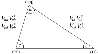
Figure 1: Sketch of the unitarity triangle.

1.2 Constraints from $K$ and $D$ decays

We know from the measurement of $\epsilon_{K}$ that CPV in the $K$ system is at the right level, as it can be accommodated in the SM with an ${\cal O}(1)$ value of the KM phase [3]. The other observed $CP$ violating quantity in kaon decay, $\epsilon_{K}^{\prime}$, is notoriously hard to calculate, so hadronic uncertainties have precluded precision tests of the KM mechanism. In the kaon sector these will come from the study of $K\to\pi\nu\bar{\nu}$ decays. The BNL E949 experiment observed the third event, yielding [5]

$${\cal B}(K^{+}\to\pi^{+}\nu\bar{\nu})=(1.47^{+1.30}_{-0.89})\times 10^{-10}\,.$$ (3)

This is consistent with the SM within the large uncertainties, but much more statistics is needed to make definitive tests.

The $D$ meson system is complementary to $K$ and $B$ mesons, because flavor and $CP$ violation are suppressed both by the GIM mechanism and by the Cabibbo angle. Therefore, CPV in $D$ decays, rare $D$ decays, and $D-\,\overline{\!D}$ mixing are predicted to be small in the SM and have not been observed. The $D^{0}-\,\overline{\!D}{}^{0}$ is the only neutral meson mixing generated by down-type quarks in the SM (up-type squarks in SUSY). The strongest hint for $D^{0}-\,\overline{\!D}{}^{0}$ mixing is [6]

$$y_{CP} = {\Gamma(CP\mbox{ even})-\Gamma(CP\mbox{ odd})\over\Gamma(CP\mbox{ even})+\Gamma(CP\mbox{ odd})}$$ (4)

$$= (0.9\pm 0.4)\%\,.$$

Unfortunately, because of hadronic uncertainties, this measurement cannot be interpreted as a sign of new physics [7]. At the present level of sensitivity, CPV would be the only clean signal of NP in the $D$ sector.

2 $CP$ violation in $B$ decays and $B\to J/\psi K_{S}$

2.1 $CP$ violation in decay

$CP$ violation in decay is in some sense its simplest form, and can be observed in both charged and neutral meson as well as in baryon decays. It requires at least two amplitudes with nonzero relative weak $(\phi_{k})$ and strong $(\delta_{k})$ phases to contribute to a decay,

$$A_{f} = \langle f|{\cal H}|B\rangle=\sum_{k}A_{k}\,e^{i\delta_{k}}\,e^{i\phi_{k}}\,,$$

$$\overline{A}_{\overline{f}} = \langle\overline{f}|{\cal H}|\,\overline{\!B}\rangle=\sum_{k}A_{k}\,e^{i\delta_{k}}\,e^{-i\phi_{k}}\,.$$ (5)

If $|{\overline{A}_{\overline{f}}/A_{f}}|\neq 1$ then $CP$ is violated.

This type of $CP$ violation is unambiguously observed in the kaon sector by $\epsilon^{\prime}_{K}\neq 0$, and now it is also established in $B$ decays with $5.7\sigma$ significance,

$$A_{K^{-}\pi^{+}} \equiv {\Gamma(\,\overline{\!B}\to K^{-}\pi^{+})-\Gamma(B\to K^{+}\pi^{-})\over\Gamma(\,\overline{\!B}\to K^{-}\pi^{+})+\Gamma(B\to K^{+}\pi^{-})}$$ (6)

$$= -0.109\pm 0.019\,,$$

averaging the BABAR [8], BELLE [9], CDF [10], and CLEO [11] measurements. This is simply a counting experiment: there are a significantly larger number of $B^{0}\to K^{+}\pi^{-}$ than $\,\overline{\!B}{}^{0}\to K^{-}\pi^{+}$ decays.

This measurement implies that after the “$K$-superweak” model [12], now also “$B$-superweak” models are excluded. I.e., models in which $CP$ violation in the $B$ sector only occurs in $B^{0}-\,\overline{\!B}{}^{0}$ mixing are no longer viable. This measurement also establishes that there are sizable strong phases between the tree $(T)$ and penguin $(P)$ amplitudes in charmless $B$ decays, since estimates of $|T/P|$ are not much larger than $A_{K^{-}\pi^{+}}$. (Note that a sizable strong phase has also been established in $B\to\psi K^{*}$ [13, 14].) Such information on strong phases will have broader implications for the theory of charmless nonleptonic decays and for understanding the $B\to K\pi$ and $\pi\pi$ rates discussed in Sec. 6.2.

The bottom line is that, similar to $\epsilon^{\prime}_{K}$, our theoretical understanding at present is insufficient to either prove or rule out that the $CP$ asymmetry in Eq. (6) is due to NP.

2.2 CPV in mixing

The two $B$ meson mass eigenstates are related to the flavor eigenstates via

$$|B_{L,H}\rangle=p|B^{0}\rangle\pm q|\,\overline{\!B}{}^{0}\rangle\,.$$ (7)

$CP$ is violated if the mass eigenstates are not equal to the $CP$ eigenstates. This happens if $|q/p|\neq 1$, i.e., if the physical states are not orthogonal, $\langle B_{H}|B_{L}\rangle\neq 0$, showing that this is an intrinsically quantum mechanical phenomenon.

The simplest example of this type of $CP$ violation is the semileptonic decay asymmetry to “wrong sign” leptons,

$$A_{\rm SL} = {\Gamma(\,\overline{\!B}{}^{0}(t)\to\ell^{+}X)-\Gamma(B^{0}(t)\to\ell^{-}X)\over\Gamma(\,\overline{\!B}{}^{0}(t)\to\ell^{+}X)+\Gamma(B^{0}(t)\to\ell^{-}X)}$$ (8)

$$= {1-|q/p|^{4}\over 1+|q/p|^{4}}=(-0.05\pm 0.71)\%\,,$$

implying $|q/p|=1.0003\pm 0.0035$, where this average is dominated by a new BELLE result [15]. In kaon decays the similar asymmetry has been measured [16], in agreement with the expectation that it is equal to $4\,{\rm Re}\,\epsilon$.

The calculation of $A_{\rm SL}$ is only possible from first principles in the $m_{b}\gg\Lambda_{\rm QCD}$ limit using an operator product expansion to evaluate the relevant nonleptonic rates. The calculation has sizable uncertainties by virtue of our limited understanding of $b$ hadron lifetimes. Last year the NLO QCD calculation of $A_{\rm SL}$ was completed [17, 18], predicting $A_{\rm SL}=-(5.5\pm 1.3)\times 10^{-4}$, where I averaged the central values and quoted the larger of the two theory error estimates. (The similar asymmetry in the $B_{s}$ sector is expected to be $\lambda^{2}$ smaller.) Although the experimental error in Eq. (8) is an order of magnitude larger than the SM expectation, this measurement already constraints new physics [19], as the $m_{c}^{2}/m_{b}^{2}$ suppression of $A_{\rm SL}$ in the SM can be avoided by NP.

2.3 CPV in the interference between decay with and without mixing, $B\to J/\psi K_{S}$ and its implications

It is possible to obtain theoretically clean information on weak phases in $B$ decays to certain $CP$ eigenstate final states. The interference phenomena between $B^{0}\to f_{CP}$ and $B^{0}\to\,\overline{\!B}{}^{0}\to f_{CP}$ is described by

$$\lambda_{f_{CP}}=\frac{q}{p}\,\frac{\overline{A}_{f_{CP}}}{A_{f_{CP}}}=\eta_{f_{CP}}\,\frac{q}{p}\,\frac{\overline{A}_{f_{CP}}}{A_{\overline{f}_{CP}}}\,,$$ (9)

where $\eta_{f_{CP}}=\pm 1$ is the $CP$ eigenvalue of $f_{CP}$. Experimentally one can study the time dependent $CP$ asymmetry,

$$a_{f_{CP}} = {\Gamma[\,\overline{\!B}{}^{0}(t)\to f]-\Gamma[B^{0}(t)\to f]\over\Gamma[\,\overline{\!B}{}^{0}(t)\to f]+\Gamma[B^{0}(t)\to f]}\qquad$$

$$= S_{f_{CP}}\sin(\Delta m\,t)-C_{f_{CP}}\cos(\Delta m\,t)\,,$$

where

$$S_{f}={2\,{\rm Im}\,\lambda_{f}\over 1+|\lambda_{f}|^{2}}\,,\quad C_{f}(=-A_{f})={1-|\lambda_{f}|^{2}\over 1+|\lambda_{f}|^{2}}\,.$$ (11)

If amplitudes with one weak phase dominate a decay then $a_{f_{CP}}$ measures a phase in the Lagrangian theoretically cleanly. In this case $C_{f}=0$, and $a_{f_{CP}}={\rm Im}\,\lambda_{f}\,\sin(\Delta m\,t)$, where ${\rm arg}\lambda_{f}$ is the phase difference between the two decay paths (with or without mixing).

The theoretically cleanest example of this type of $CP$ violation is $B\to\psi K_{S}$. While there are tree and penguin contributions to the decay with different weak phases, the dominant part of the penguin amplitudes have the same weak phase as the tree amplitude. Therefore, contributions with the tree amplitude’s weak phase dominate, to an accuracy better than $\sim$1%. In the usual phase convention ${\rm arg}\,\lambda_{\psi K_{S}}=(B\mbox{-mixing}=2\beta)+(\mbox{decay}=0)+(K\mbox{-mixing}=0)$, so we expect $S_{\psi K}=\sin 2\beta$ and $C_{\psi K}=0$ to a similar accuracy. The new world average is

$$\sin 2\beta=0.726\pm 0.037\,,$$ (12)

which is now a 5% measurement. For the first time $\cos 2\beta$ has also been constrained, by studying angular distributions in the time dependent $B\to\psi K^{*0}$ analysis. BABAR obtained [13] $\cos 2\beta=+2.72^{+0.50}_{-0.79}\pm 0.27$, excluding the negative $\cos 2\beta$ solution at the 89% CL. With more data, this will eliminate 2 of the 4 discrete ambiguities, corresponding to $\beta=(\pi-\arcsin S_{\psi K})/2$ and $\beta=(3\pi-\arcsin S_{\psi K})/2$.

$S_{\psi K}$ was the first observation of $CP$ violation outside the kaon sector, and the first observation of an ${\cal O}(1)$ effect that violates $CP$. It implies that models with approximate $CP$ symmetry (in the sense that all CPV phases are small) are excluded. The constraints on the CKM matrix from the measurements of $S_{\psi K}$, $|V_{ub}/V_{cb}|$, $\epsilon_{K}$, $B$ and $B_{s}$ mixing are shown in Fig. 2 using the CKMfitter package [20, 21]. The overall consistency between these measurements constitutes the first precise test of the CKM picture. It also implies that it is unlikely that we will find ${\cal O}(1)$ deviations from the SM, and we should look for corrections rather than alternatives of the CKM picture.

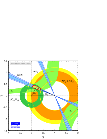
Figure 2: The present CKM fit.

3 Other $CP$ asymmetries that are approximately $\sin 2\beta$ in the SM

Table 1: $CP$ asymmetries for which the SM predicts $-\eta_{f}S_{f}\approx\sin 2\beta$. The 3rd column contains my estimates of limits on the deviations from $\sin 2\beta$ in the SM (strict bounds are worse), and the last two columns show the world averages [25]. (The $CP$-even fractions in $K^{+}K^{-}K_{S}$ and $D^{*+}D^{*-}$ are determined experimentally.)

Dominant final SM upper limit on $-\eta_{f_{CP}}S_{f_{CP}}$ $C_{f_{CP}}$ process state $|-\eta_{f_{CP}}S_{f_{CP}}-\sin 2\beta|$ $b\to c\bar{c}s$ $\psi K_{S}$ $<0.01$ $+0.726\pm 0.037$ $+0.031\pm 0.029$ $b\to c\bar{c}d$ $\psi\pi^{0}$ $\sim 0.2$ $+0.40\pm 0.33$ $+0.12\pm 0.24$ $D^{*+}D^{*-}$ $\sim 0.2$ $+0.20\pm 0.32$ $+0.28\pm 0.17$ $b\to s\bar{q}q$ $\phi K^{0}$ $\sim 0.05$ $+0.34\pm 0.20$ $-0.04\pm 0.17$ $\eta^{\prime}K_{S}$ $\sim 0.1$ $+0.41\pm 0.11$ $-0.04\pm 0.08$ $K^{+}K^{-}K_{S}$ $\sim 0.15$ $+0.53\pm 0.17$ $+0.09\pm 0.10$ $\pi^{0}K_{S}$ $\sim 0.15$ $+0.34\pm 0.28$ $+0.09\pm 0.14$ $f_{0}K_{S}$ $\sim 0.15$ $+0.39\pm 0.26$ $+0.14\pm 0.22$ $\omega K_{S}$ $\sim 0.15$ $+0.75\pm 0.66$ $-0.26\pm 0.50$

The $b\to s$ transitions, such as $B\to\phi K_{S}$, $\eta^{\prime}K_{S}$, $K^{+}K^{-}K_{S}$, etc., are dominated by one-loop (penguin) diagrams in the SM, and therefore new physics could compete with the SM contributions [22]. Using CKM unitarity we can write the contributions to such decays as a term proportional to $V_{cb}V_{cs}^{*}$ and another proportional to $V_{ub}V_{us}^{*}$. Since their ratio is ${\cal O}(\lambda^{2})\sim 0.05$, we expect amplitudes with one weak phase to dominate these decays as well. Thus, in the SM, the measurements of $-\eta_{f}S_{f}$ should agree with each other and with $S_{\psi K}$ to an accuracy of order $\lambda^{2}\sim 0.05$.

If there is a SM and a NP contribution, the asymmetries depend on their relative size and phase, which depend on hadronic matrix elements. Since these are mode-dependent, the asymmetries will, in general, be different between the various modes, and different from $S_{\psi K}$. One may also find $C_{f}$ substantially different from 0. (NP would have to dominate over the SM amplitude in order that the asymmetries become different from the SM and equal to one other.)

The averages of the latest BABAR [23] and BELLE [24] results are shown in Table 1. The two data sets are more consistent than before, so averaging them seems meaningful at this time. The single largest deviation from the SM is in the $\eta^{\prime}K_{S}$ mode,

$$S_{\psi K}-S_{\eta^{\prime}K_{S}}=0.31\pm 0.12\,,$$ (13)

which is $2.6\sigma$. The average $CP$ asymmetry in all $b\to s$ modes, which also equals $S_{\psi K}$ in the SM, has a more significant deviation,

$$S_{\psi K}-\langle-\eta_{f}S_{f(b\to s)}\rangle=0.30\pm 0.08\,.$$ (14)

This $3.5\sigma$ effect comes from $2.7\sigma$ at BABAR and $2.4\sigma$ at BELLE. It is a less than $3.5\sigma$ signal for NP, because some of the modes included may deviate significantly from $S_{\psi K}$ in the SM. However, there is another $3.1\sigma$ effect,

$$S_{\psi K}-\langle S_{\eta^{\prime}K_{S},\phi K_{S}}\rangle=0.33\pm 0.11\,.$$ (15)

The entries in the third column in Table 1 show my estimates of limits on the deviations from $S_{\psi K}$ in the SM. The hadronic matrix elements multiplying the generic ${\cal O}(0.05)$ suppression of the “SM pollution” are hard to bound model independently [26], so strict bounds are weaker, while model calculations tend to obtain smaller limits. I attempted to list reasonable benchmarks for each mode.

3.1 Implications of the data

To understand the significance of Eq. (13) and (15), note that a conservative bound using $SU(3)$ flavor symmetry and (updated) experimental limits on related modes gives [26, 27] $|S_{\psi K}-S_{\eta^{\prime}K_{S}}|<0.2$ in the SM. Most other estimates obtain bounds a factor of two smaller or even better (these are also more model dependent). Thus we can be confident that, if established at the $5\sigma$ level, $S_{\eta^{\prime}K_{S}}\approx 0.4$ would be a sign of NP. (The deviation of $S_{\phi K_{S}}$ from $S_{\psi K}$ is now less than $2\sigma$, but there is room for discovery, as the present central value of $S_{\phi K}$ with a smaller error could still establish NP.) The largest deviation from the SM at present is the $3.5\sigma$ effect in $\langle-\eta_{f}S_{f(b\to s)}\rangle$. Such a discovery would exclude in addition to the SM, models with minimal flavor violation, and universal SUSY models, such as gauge mediated SUSY breaking.

In the last few years the central value of $S_{\phi K_{S}}$ got closer to $S_{\psi K}$, while $S_{\eta^{\prime}K_{S}}$ got further from it, disfavoring models in which NP enters $S_{\phi K_{S}}$ but not $S_{\eta^{\prime}K_{S}}$. This includes models of parity-even NP, which would affect $B\to\phi K_{S}$ (odd $\to$ odd) but not $B\to\eta^{\prime}K_{S}$ (odd $\to$ even). This happens, for example, in a left-right-symmetric SUSY model, if the LRS breaking scale is high enough so that direct effects from the $W_{R}$ sector are absent [28]. This scenario is disfavored also because the $K^{+}K^{-}K_{S}$ final state is $P$-odd, just like $\phi K_{S}$.

Model building may actually become more interesting with the new data. The present central values of $S_{\eta^{\prime}K_{S}}$ and $S_{\phi K_{S}}$ can be reasonably accommodated with NP, such as SUSY (unlike ${\cal O}(1)$ deviations from $S_{\psi K_{S}}$). While $B\to X_{s}\gamma$ mainly constrains $LR$ mass insertions, penguins shown in Fig. 3 involving $RR$ (and $LL$) mass insertions can give sizable effect in $b\to s$ transitions. However, as of this conference, we also know that ${\cal B}(B\to X_{s}\ell^{+}\ell^{-})=(4.5\pm 1.0)\times 10^{-6}$ agrees with the SM at the ${\cal O}(20\%)$ level [25], which gives new constraints on the $RR$ and $LL$ mass insertions (replace $g\to Z$ and $s\bar{s}\to\ell^{+}\ell^{-}$).

Figure 3: A SUSY contribution to $b\to s\bar{s}s$ [29].

4 Measurements of $\alpha$ and $\gamma$

To clarify notation, I’ll call a $\gamma$-measurement the determination of the phase difference between $b\to u$ and $b\to c$ transitions, while $\alpha$ will refer to the measurements of $\gamma$ in the presence of $B-\,\overline{\!B}$ mixing ($\alpha\equiv\pi-\beta-\gamma$). Interestingly, the methods that give the best results were not even talked about before 2003.

4.1 $\alpha$ from $B\to\pi\pi$

In contrast to $B\to\psi K$, which is dominated by amplitudes with one week phase, it is now well-established that in $B\to\pi^{+}\pi^{-}$ there are two comparable contributions with different weak phases [30]. Therefore, to determine $\alpha$ model independently, it is necessary to carry out the isospin analysis [31]. The hardest ingredient is the measurement of the $\pi^{0}\pi^{0}$ mode,

$${\cal B}(B\to\pi^{0}\pi^{0})=(1.51\pm 0.28)\times 10^{-6}\,,$$ (16)

and in particular the need to measure the $CP$-tagged rates. At this conference BABAR [32] and BELLE [9] presented the first such measurements, giving the world average

$${\Gamma(\,\overline{\!B}\to\pi^{0}\pi^{0})-\Gamma(B\to\pi^{0}\pi^{0})\over\Gamma(\,\overline{\!B}\to\pi^{0}\pi^{0})+\Gamma(B\to\pi^{0}\pi^{0})}=0.28\pm 0.39.$$ (17)

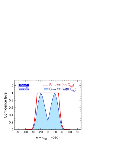
Figure 4: Constraints on $\alpha-\alpha_{\rm eff}$.

Thus, for the first time, we can determine from the isospin analysis (with sizable error) the penguin pollution, $\alpha-\alpha_{\rm eff}$ [$2\alpha_{\rm eff}\equiv{\rm arg}\,\lambda_{\pi^{+}\pi^{-}}=\arcsin(S_{\pi^{+}\pi^{-}}(1-C_{\pi^{+}\pi^{-}}^{2})^{-1/2})$]. In Fig. 4, the blue (shaded) region shows the confidence level using Eq. (17), while the red (thick solid) curve is the constraint without it. We find $|\alpha-\alpha_{\rm eff}|<37^{\circ}$ at 90% CL, a small improvement over the $39^{\circ}$ bound without Eq. (17); so it will take a lot more data to determine $\alpha$ precisely. The interpretation for $\alpha$ is unclear at present, due to the marginal consistency of the $S_{\pi^{+}\pi^{-}}$ data; see Table 2.

Table 2: $CP$ violation in $B\to\pi^{+}\pi^{-}$.

$B\to\pi^{+}\pi^{-}$ $S_{\pi^{+}\pi^{-}}$ $C_{\pi^{+}\pi^{-}}$ BABAR $-0.30\pm 0.17$ $-0.09\pm 0.15$ BELLE $-1.00\pm 0.22$ $-0.58\pm 0.17$ average $-0.61\pm 0.14$ $-0.37\pm 0.11$

4.2 $\alpha$ from $B\to\rho\rho$

$B\to\rho\rho$ is more complicated than $B\to\pi\pi$ in that a vector-vector ($VV$) final state is a mixture of $CP$-even ($L=0$ and 2) and -odd ($L=1$) components. The $B\to\pi\pi$ isospin analysis applies for each $L$ in $B\to\rho\rho$ (or in the transversity basis for each $\sigma=0,\parallel,\perp$).The situation is simplified dramatically by the experimental observation that in the $\rho^{+}\rho^{-}$ and $\rho^{+}\rho^{0}$ modes the longitudinal polarization fraction is near unity (see Sec. 6.1), so the $CP$-even fraction dominates. Thus, one can simply bound $\alpha-\alpha_{\rm eff}$ from [33]

$${\cal B}(B\to\rho^{0}\rho^{0})<1.1\times 10^{-6}\ (90\%\ {\rm CL})\,.$$ (18)

The smallness of this rate implies that $\alpha-\alpha_{\rm eff}$ in $B\to\rho\rho$ is much smaller than in $B\to\pi\pi$. To indicate the difference, note that ${{\cal B}(B\to\pi^{0}\pi^{0})/{\cal B}(B\to\pi^{+}\pi^{0})}=0.27\pm 0.06$, while ${{\cal B}(B\to\rho^{0}\rho^{0})/{\cal B}(B\to\rho^{+}\rho^{0})}<0.04\ \ (90\%\ {\rm CL})$. From $S_{\rho^{+}\rho^{-}}$ and the isospin bound on $\alpha-\alpha_{\rm eff}$ BABAR obtains [33]

$$\alpha=96\pm 10\pm 4\pm 11^{\circ}(\alpha-\alpha_{\rm eff})\,.$$ (19)

Ultimately the isospin analysis is more complicated in $B\to\rho\rho$ than in $\pi\pi$, because the nonzero value of $\Gamma_{\rho}$ allows for the final state to be in an isospin-1 state [34]. This only affects the results at the ${\cal O}(\Gamma_{\rho}^{2}/m_{\rho}^{2})$ level, which is smaller than other errors at present. With higher statistics, it will be possible to constrain this effect using the data [34].

4.3 $\alpha$ from $B\to\rho\pi$

In the two-body analysis isospin symmetry gives two pentagon relations [35]. Solving them would require measurements of the rates and $CP$ asymmetries in all the $B\to\rho^{+}\pi^{-}$, $\rho^{-}\pi^{+}$, and $\rho^{0}\pi^{0}$ modes, which is not available. While BABAR set a 90% CL upper bound [36] ${\cal B}(B\to\rho^{0}\pi^{0})<2.9\times 10^{-6}$, BELLE measured [37] ${\cal B}(B\to\rho^{0}\pi^{0})=(5.1\pm 1.6\pm 0.9)\times 10^{-6}$. The two experiments agree on the direct $CP$ asymmetries [32, 38], and their average

$$A_{\pi^{-}\rho^{+}} = -0.48^{+0.13}_{-0.14}\,,$$

$$A_{\pi^{+}\rho^{-}} = -0.15\pm 0.09\,,$$ (20)

is $3.6\sigma$ from no direct $CP$ violation, $(A_{\pi^{-}\rho^{+}},$ $A_{\pi^{+}\rho^{-}})=(0,0)$. With assumptions about factorization and $SU(3)$ flavor symmetry, one can obtain $\alpha=(95\pm 6_{\rm(exp)}\pm 15_{\rm(th)})^{\circ}$ [39], but here the error is theory dominated.

At this conference BABAR showed the first Dalitz plot analysis [40] of the the interference regions in $B\to\pi^{+}\pi^{-}\pi^{0}$ to determine [32]

$$\alpha=(113^{+27}_{-17}\pm 6)^{\circ},$$ (21)

which uses less assumptions than the extraction of $\alpha$ from the two-body measurements.

4.4 Combined determination of $\alpha$

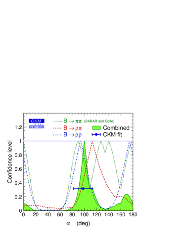
Figure 5: Confidence levels of the $\alpha$ measurements.

The combination of these measurements of $\alpha$ is shown in Fig. 5. Due to the marginal consistency of the $S_{\pi^{+}\pi^{-}}$ data, I quote the average of $S_{\rho^{+}\rho^{-}}$ and the $\rho\pi$ Dalitz analysis,

$$\alpha=(103\pm 11)^{\circ}.$$ (22)

Including $\alpha$ extracted from $B\to\pi\pi$ would make only a small difference at present, shifting $\alpha$ to $(100^{+12}_{-10})^{\circ}$. It is interesting to note that the direct determination of $\alpha$ in Eq. (22) is already more precise than it is from the CKM fit, which gives $\alpha=(98\pm 16)^{\circ}$.

4.5 $\gamma$ from $B^{\pm}\to DK^{\pm}$

The idea is to measure the interference of $B^{-}\to D^{0}K^{-}$ ($b\to c\bar{u}s$) and $B^{-}\to\,\overline{\!D}{}^{0}K^{-}$ ($b\to u\bar{c}s$) transitions, which can be studied in final states accessible in both $D^{0}$ and $\,\overline{\!D}{}^{0}$ decays [41, 42]. In principle, it is possible to extract the $B$ and $D$ decay amplitudes, the relative strong phases, and the weak phase $\gamma$ from the data.

A practical complication is that the amplitude ratio

$$r_{B}\equiv{A(B^{-}\to\,\overline{\!D}{}^{0}K^{-})\over A(B^{-}\to D^{0}K^{-})}\,$$ (23)

is expected to be small. To make the two interfering amplitudes comparable in size, the ADS method [43] was proposed to study final states where Cabibbo-allowed and doubly Cabibbo-suppressed $D$ decays interfere. While this method is being pursued experimentally, some other recently proposed variants may also be worth a closer look. If $r_{B}$ is not much below $\sim$0.2, then studying singly Cabibbo-suppressed $D$ decays may be advantageous, such as $B^{\pm}\to K^{\pm}(KK^{*})_{D}$ [44]. In three-body $B$ decays the color suppression of one of the amplitudes can be avoided [45].

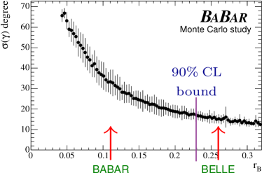
Figure 6: Monte Carlo study of the correlation of $r_{B}$ and the error of $\gamma$ [46]. The central values of the BABAR and BELLE measurements are shown, together with an upper bound from the ADS analysis.

It was recently realized [47, 48] that both $D^{0}$ and $\,\overline{\!D}{}^{0}$ have Cabibbo-allowed decays to certain 3-body final states, such as $K_{S}\pi^{+}\pi^{-}$. This analysis has only a two-fold discrete ambiguity, and one can integrate over regions of the Dalitz plot, potentially enhancing the sensitivity. The best present determination of $\gamma$ comes from this analysis. BELLE obtained from 140 ${\rm fb}^{-1}$ data [49]

$$\gamma=77^{+17}_{-19}\pm 13\pm 11^{\circ}(model)\,,$$ (24)

while BABAR found from 191 ${\rm fb}^{-1}$ data [46]

$$\gamma=88\pm 41\pm 19\pm 10^{\circ}(model)\,.$$ (25)

The sizable difference in the errors in these measurements is due to the large correlation between the error of $\gamma$ and the value of $r_{B}$, as shown in Fig. 6. While BELLE found [50] $r_{B}=0.26^{+0.11}_{-0.15}\pm 0.03\pm 0.04$, BABAR obtained $r_{B}<0.18$ (90% CL), with the central values shown in Fig. 6. From the ADS analyses 90% CL upper bounds on $r_{B}$ were obtained, $r_{B}<0.23$ at BABAR [46] and $r_{B}<0.28$ at BELLE [50]. These analyses are consistent with each other at the $1-1.5\sigma$ level, but it will take more data to pin down $r_{B}$ and determine $\gamma$ more precisely.

5 Implications of the first $\alpha$ and $\gamma$ measurements

Since the goal of the $B$ factories is to overconstrain the CKM matrix, one should include in the CKM fit all measurements that are not limited by theoretical uncertainties. The result of such a fit is shown in Fig. 7, which includes in addition to the inputs in Fig. 2 the following: (i) $\alpha$ from $B\to\rho\rho$ and from the $\rho\pi$ Dalitz analysis, (ii) $\gamma$ from $B\to DK$ (with $D\to K_{S}\pi^{+}\pi^{-}$), and (iii) $2\beta+\gamma$ from $B\to D^{(*)\pm}\pi^{\mp}$ measurements.

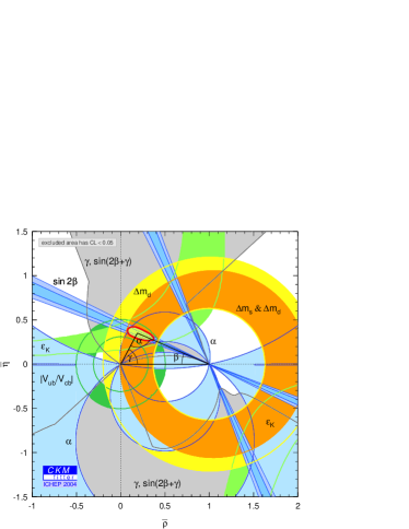
Figure 7: CKM fits including $\alpha$ and $\gamma$ measurements.

The best fit region in Fig. 7 shrinks only slightly compared to Fig. 2. An interesting consequence of the new fit is a noticeable reduction in the allowed range of $B_{s}-\,\overline{\!B}_{s}$ mixing. While the standard CKM fit gives $\Delta m_{s}=\big{(}17.9^{+10.5}_{-1.7}\,{}^{[+20.0]}_{[-2.8]}\big{)}\,{\rm ps}^{-1}$ at $1\sigma\ [2\sigma]$, the new fit gives $\Delta m_{s}=\big{(}17.9^{+7.4}_{-1.4}\,{}^{[+13.3]}_{[-2.7]}\big{)}\,{\rm ps}^{-1}$.

5.1 New physics in $B^{0}-\,\overline{\!B}{}^{0}$ mixing

      

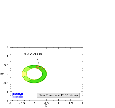
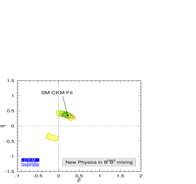
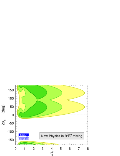
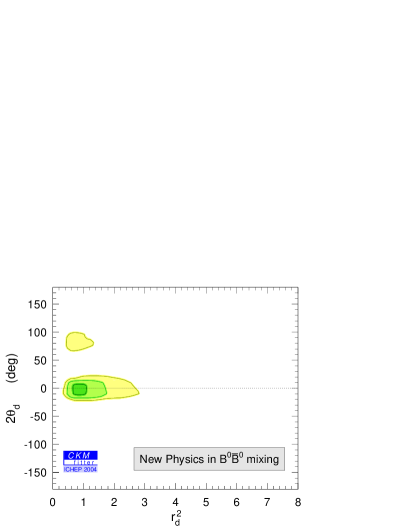
Figure 8: Allowed regions in the $\rho-\eta$ plane (top) and the $r_{d}^{2}-2\theta_{d}$ plane (bottom) in the presence of new physics in $B-\,\overline{\!B}$ mixing. The left [right] plots are the allowed regions without [with] the new constraints on $\alpha$, $\gamma$, $\cos 2\beta$, and $2\beta+\gamma$. The dark, medium, and light shaded areas have CL $>$ 0.90, 0.32, and 0.05, respectively.

These new measurements give powerful constrain new physics. In a large class of models the dominant NP effect is to modify the $B^{0}-\,\overline{\!B}{}^{0}$ mixing amplitude, that can be parameterized [51] as $M_{12}=M_{12}^{\rm(SM)}r_{d}^{2}\,e^{2i\theta_{d}}$. Then, e.g., $\Delta m_{B}=r_{d}^{2}\,\Delta m_{B}^{\rm(SM)}$, $S_{\psi K}=\sin(2\beta+2\theta_{d})$, $S_{\rho^{+}\rho^{-}}=\sin(2\alpha-2\theta_{d})$, while $|V_{ub}/V_{cb}|$ and $\gamma$ extracted from $B\to DK$ are tree-level measurements which are unaffected. Since $\theta_{d}$ drops out from $\alpha+\beta$, the measurements of $\alpha$, together with $\beta$, are effectively equivalent in these models to NP-independent measurements of $\gamma$ (up to discrete ambiguities).

Figure 8 shows the fit results using only $|V_{ub}/V_{cb}|$, $\Delta m_{B}$, $S_{\psi K}$, and $A_{\rm SL}$ as inputs (left) and also including the measurements of $\alpha$, $\gamma$, $\cos 2\beta$, and $2\beta+\gamma$ (right) in the $\rho-\eta$ plane (top) and the $r_{d}^{2}-2\theta_{d}$ plane (bottom). The new data determines $\rho$ and $\eta$ from (effectively) tree-level $B$ decays, independent of mixing, and agrees with the other SM constraints. The allowed region in the $r_{d}^{2}-2\theta_{d}$parameter space has shrunk immensely. The somewhat disfavored “non-SM region” around $2\theta_{d}\sim 80^{\circ}$ (CL $<20\%$) is due to the $\eta<0$ region in the top right plot and discrete ambiguities. Thus, NP in $B^{0}-\,\overline{\!B}{}^{0}$ mixing is severely constrained now for the first time.

6 Theoretical developments

$B$ physics is not only a great place to look for new physics, it also allows us to study the interplay of weak and strong interactions in the SM at a level of unprecedented detail. There are many observables very sensitive to NP, and the question is whether we can disentangle possible signals of NP from the hadronic physics. In the last few years there has been significant progress toward a model independent theory of certain exclusive nonleptonic decays in the $m_{B}\gg\Lambda_{\rm QCD}$ limit.

While the theory of nonleptonic $B$ decays is most developed for heavy-to-heavy decays of the type $B\to D^{(*)}\pi$ [52, 53, 54] and $\Lambda_{b}\to\Lambda_{c}\pi$ or $\Sigma_{c}\pi$ [55], here we concentrate on charmless $B$ decays, as these are the most sensitive to new physics. There are several approaches. The soft form factor and hard scattering contributions are of the same order in the $1/m_{b}$ power counting. Both Beneke et al. [56] and Keum et al. [57] make assumptions about the $\alpha_{s}$ suppression of one or the other term. An SCET [58] analysis finds the two terms comparable [59], but predictive power is retained.

One of the most contentious issues is the role of charm penguins [60], and whether strong phases are small. ($A_{K^{-}\pi^{+}}$ in Eq. (6) tells us that some strong phases are large.) As far as I can tell, no suppression of the long distance part of charm penguins has been proven. In the absence of such a proof, we should view this as a nonperturbative ${\cal O}(1)$ term that can give rise to many “unexpected” things, such as strong phases [59]. (Note that whether one talks about “long distance charm loops”, “charming penguins”, or “$D\,\overline{\!D}$ rescattering”, it’s all the same thing with different names.)

6.1 Polarization in charmless $B\to VV$

It has been argued [61] that the chiral structure of the SM and the heavy quark limit imply that charmless $B$ decays to a pair of vector mesons, such as $B\to\phi K^{*}$, $\rho\rho$, and $\rho K^{*}$ must have longitudinal polarization fractions near unity, $f_{L}=1-{\cal O}(1/m_{b}^{2})$. It is now well-established (see Table 3) that in the penguin dominated $\phi K^{*}$ modes $f_{L}\approx 0.5$. We would like to know if this is consistent with the SM.

Table 3: Longitudinal polarization fractions in charmless $B\to VV$ decays [62, 63].

$B$ decay Longitudinal polarization BELLE BABAR $\rho^{-}\rho^{+}$ $0.99^{+0.05}_{-0.04}$ $\rho^{0}\rho^{+}$ $0.95\pm 0.11$ $0.97^{+0.06}_{-0.08}$ $\omega\rho^{+}$ $0.88^{+0.12}_{-0.15}$ $\rho^{0}K^{*+}$ $0.96^{+0.06}_{-0.16}$ $\rho^{-}K^{*0}$ $0.50\pm 0.20$ $0.79\pm 0.09$ $\phi K^{*0}$ $0.52\pm 0.08$ $0.52\pm 0.05$ $\phi K^{*+}$ $0.49\pm 0.14$ $0.46\pm 0.12$

Recently several explanations were proposed why the data may be consistent with the SM [59, 61, 64, 65]. In SCET the charm penguins, if they indeed have an unsuppressed long distance part, can explain the data [59]. The $D_{s}^{(*)}D^{(*)}$ rescattering [64] can be viewed as a model calculation of this effect. It has also been argued that there are large ${\cal O}(1/m^{2})$ effects from annihilation graphs [61]; however, if this is to explain an ${\cal O}(1)$ effect in $f_{L}$ then the validity of the whole expansion should be questioned. Unfortunately it may be difficult to experimentally distinguish between these two proposals, as they appear to enter different rates in the same ratios.

While the $f_{L}(\phi K^{*})$ data may be a result of a new physics contribution (just like $A_{K^{-}\pi^{+}}$), we cannot rule out at present that it is simply due to SM physics.

6.2 $B\to K\pi$ branching ratios and $CP$ asymmetries

$B\to K\pi$ decays are sensitive to the interference of $b\to s$ penguin and $b\to u$ tree processes (and possible new physics). The SM contributions that interfere have different weak and possibly different strong phases, so the challenge is if one can make sufficiently precise predictions to do sensitive tests.

Table 4: World average $CP$-averaged $B\to\pi K$ branching ratios, and $CP$ asymmetries.

Decay mode ${\cal B}\ [10^{-6}]$ $A_{CP}$ $\,\overline{\!B}{}^{0}\to\pi^{+}K^{-}$ $18.2\pm 0.8$ $-0.11\pm 0.02$ $B^{-}\to\pi^{0}K^{-}$ $12.1\pm 0.8$ $+0.04\pm 0.04$ $B^{-}\to\pi^{-}\,\overline{\!K}{}^{0}$ $24.1\pm 1.3$ $-0.02\pm 0.03$ $\,\overline{\!B}{}^{0}\to\pi^{0}\,\overline{\!K}{}^{0}$ $11.5\pm 1.0$ $+0.00\pm 0.16$

The world average branching ratios and $CP$ asymmetries are shown in Table 4. Besides the $5.7\sigma$ measurement of $A_{K^{-}\pi^{+}}$, another interesting feature of the data is the $3.3\sigma$ difference, $A_{K^{-}\pi^{0}}-A_{K^{-}\pi^{+}}=0.15\pm 0.04$. This implies, assuming the SM, that “color-allowed” tree amplitudes do not dominate over “color-suppressed” trees (plus electroweak penguins). While this may be a challenge for some approaches, in SCET it is natural that color-allowed and -suppressed trees are comparable in charmless $B$ decays [59].

Concerning the branching ratios, I have been warned by several experimentalists that their interpretation should be handled with care. There are four ratios that have been extensively discussed in the literature [67, 68, 69, 70, 71, 72, 73, 74],

$$R_{c} \equiv 2\,\frac{{\cal B}(B^{+}\to\pi^{0}K^{+})+{\cal B}(B^{-}\to\pi^{0}K^{-})}{{\cal B}(B^{+}\to\pi^{+}K^{0})+{\cal B}(B^{-}\to\pi^{-}\,\overline{\!K}{}^{0})}$$

$$= 1.004\pm 0.084\,,$$

$$R_{n} \equiv \frac{1}{2}\,\frac{{\cal B}(B^{0}\to\pi^{-}K^{+})+{\cal B}(\,\overline{\!B}{}^{0}\to\pi^{+}K^{-})}{{\cal B}(B^{0}\to\pi^{0}K^{0})+{\cal B}(\,\overline{\!B}{}^{0}\to\pi^{0}\,\overline{\!K}{}^{0})}$$

$$= 0.789\pm 0.075\,,$$

$$R \equiv \frac{\Gamma(B^{0}\to\pi^{-}K^{+})+\Gamma(\,\overline{\!B}{}^{0}\to\pi^{+}K^{-})}{\Gamma(B^{+}\to\pi^{+}K^{0})+\Gamma(B^{-}\to\pi^{-}\,\overline{\!K}{}^{0})}$$

$$= 0.820\pm 0.056\,,$$

$$R_{L} \equiv 2\,\frac{\bar{\Gamma}(B^{-}\to\pi^{0}K^{-})+\bar{\Gamma}(\,\overline{\!B}{}^{0}\to\pi^{0}\,\overline{\!K}{}^{0})}{\bar{\Gamma}(B^{-}\to\pi^{-}\,\overline{\!K}{}^{0})+\bar{\Gamma}(\,\overline{\!B}{}^{0}\to\pi^{+}K^{-})}$$ (26)

$$= 1.123\pm 0.070\,,$$

where $\Gamma\equiv{\cal B}/\tau$, and $\bar{\Gamma}$ in the last equation denotes the $CP$-averaged widths. These ratios are interesting, as their deviations from unity are sensitive to different corrections to the dominant penguin amplitudes.

The pattern of these ratios is quite different from what it was before ICHEP: $R_{c}$ and $R_{L}$ became significantly closer to unity, while $R$’s deviation from unity increased. This seems to disfavor new physics explanations [74, 69], according to which NP primarily modifies electroweak penguin contributions. This is because electroweak penguins are color allowed in the modes involving $\pi^{0}$’s, that enter $R_{c}$, while they are color suppressed in the other ones, such as those in $R$.

Since $R$ is significantly below unity, at present the Fleischer-Mannel bound [67] is interesting again, giving $\gamma<75^{\circ}$ (95% CL).

It will be fascinating to understand the theory in sufficient detail to sort out what the data is telling us, and also to see where the measurements will settle.

7 Outlook

Table 5: Some interesting measurement that are far from being theory limited. The errors for the $CP$ asymmetries in the first box refer to the angles in parenthesis, assuming typical values for other parameters.

Measurement (in SM) Theoretical limit Present error $B\to\psi K_{S}$  ($\beta$) $\sim 0.2^{\circ}$ $1.6^{\circ}$ $B\to\phi K_{S},\ \eta^{(\prime)}K_{S}$, … ($\beta$) $\sim 2^{\circ}$ $\sim 10^{\circ}$ $B\to\pi\pi,\ \rho\rho,\ \rho\pi$  ($\alpha$) $\sim 1^{\circ}$ $\sim 15^{\circ}$ $B\to DK$  ($\gamma$) $\ll 1^{\circ}$ $\sim 25^{\circ}$ $B_{s}\to\psi\phi$  ($\beta_{s}$) $\sim 0.2^{\circ}$ — $B_{s}\to D_{s}K$  ($\gamma-2\beta_{s}$) $\ll 1^{\circ}$ — $|V_{cb}|$ $\sim 1\%$ $\sim 3\%$ $|V_{ub}|$ $\sim 5\%$ $\sim 15\%$ $B\to X_{s}\gamma$ $\sim 5\%$ $\sim 10\%$ $B\to X_{s}\ell^{+}\ell^{-}$ $\sim 5\%$ $\sim 20\%$ $B\to X_{s}\nu\bar{\nu},K^{(*)}\nu\bar{\nu}$ $\sim 5\%$ — $K^{+}\to\pi^{+}\nu\bar{\nu}$ $\sim 5\%$ $\sim 70\%$ $K_{L}\to\pi^{0}\nu\bar{\nu}$ $<1\%$ —

Having seen these impressive measurements, one should ask where we go from here in flavor physics? Whether we see in the next few years stronger signals of flavor physics beyond the SM will certainly be decisive [75]. The existing measurements could have shown deviations from the SM, and if there are new particles at the TeV scale, new flavor physics could show up “any time”. In fact, we do not know whether we are seeing hints or just statistical fluctuations in the $S_{b\to s}$ data.

For BABAR and BELLE, reducing the error of $S_{\psi K}$ to the few percent level has been a well-defined target. The data sets have roughly doubled each year for the past several years, and will reach $500-1000\,{\rm fb}^{-1}$ each in a few years, possibly allowing for unambiguous observation of NP if the central values do not change too much. If NP is seen in flavor physics then we will certainly want to study it in as many different processes as possible. If NP is not seen in flavor physics, then it is interesting to achieve what is theoretically possible, thereby testing the SM at a much more precise level. Even in the latter case, flavor physics will give powerful constraints on model building in the LHC era.

The present status and (my estimates of) the theoretical limitations of some of the theoretically cleanest measurements are summarized in Table 5. It shows that the sensitivity to NP is not limited by hadronic physics in many measurements for a long time to come. One cannot overemphasize that the program as a whole is a lot more interesting than any single measurement, since it is the multitude of “overconstraining” measurements and their correlations that are likely to carry the most interesting information.

8 Conclusions

The large number of impressive new results speak for themselves, so it is easy to summarize the main lessons we have learned:

• $\sin 2\beta=0.726\pm 0.037$
  implies that the overall consistency of the SM is very good, and the KM phase is probably the dominant source of CPV in flavor changing processes;

• $S_{\psi K}-\langle-\eta_{f}S_{f(b\to s)}\rangle=0.30\pm 0.08\ (3.5\sigma)$ and $S_{\psi K}-S_{\eta^{\prime}K_{S}}=0.31\pm 0.12\ (2.6\sigma)$
  imply that we may be observing hints of NP in $b\to s$ transitions, since the present central values with $5\sigma$ would be quite convincing;

• $A_{K^{-}\pi^{+}}=-0.11\pm 0.02\ (5.7\sigma)$
  implies that “$B$-superweak” models are excluded and that there are large strong phases in some charmless $B$ decays;

• First measurements of $\alpha$ and $\gamma$
  imply that the direct measurement of $\alpha$ is already more precise than the indirect CKM fit, and finally we have severe constraints on NP in $B-\,\overline{\!B}$ mixing.

References

- [1] J. H. Christenson, J. W. Cronin, V. L. Fitch and R. Turlay, Phys. Rev. Lett. 13 (1964) 138.
- [2] N. Cabibbo, Phys. Rev. Lett. 10 (1963) 531.
- [3] M. Kobayashi and T. Maskawa, Prog. Theor. Phys. 49 (1973) 652.
- [4] For recent reviews, see: Z. Ligeti, eConf C020805 (2002) L02 [hep-ph/0302031]; Y. Nir, hep-ph/0109090.
- [5] V. V. Anisimovsky et al. [E949 Collaboration], hep-ex/0403036.
- [6] B. D. Yabsley, Int. J. Mod. Phys. A 19 (2004) 949 [hep-ex/0311057].
- [7] A. F. Falk, Y. Grossman, Z. Ligeti and A. A. Petrov, Phys. Rev. D 65 (2002) 054034 [hep-ph/0110317]; A. F. Falk et al., Phys. Rev. D 69 (2004) 114021 [hep-ph/0402204].
- [8] B. Aubert [BaBar Collaboration], hep-ex/0407057.
- [9] Y. Chao, talk at this conference.
- [10] CDF Collaboration, CDF note available: http://www–cdf.fnal.gov/physics/ new/bottom/040722.blessed–bhh.
- [11] S. Chen et al. [CLEO Collaboration], Phys. Rev. Lett. 85 (2000) 525 [hep-ex/0001009].
- [12] L. Wolfenstein, Phys. Rev. Lett. 13 (1964) 562.
- [13] M. Verderi [BABAR Collaboration], hep-ex/0406082.
- [14] T. Higuchi, talk at this conference.
- [15] K. Abe et al. [Belle Collaboration], hep-ex/0409012.
- [16] A. Angelopoulos et al. [CPLEAR Collaboration], Phys. Lett. B 444 (1998) 43.
- [17] M. Beneke, G. Buchalla, A. Lenz and U. Nierste, Phys. Lett. B 576 (2003) 173 [hep-ph/0307344].
- [18] M. Ciuchini et al., JHEP 0308 (2003) 031 [hep-ph/0308029].
- [19] S. Laplace, Z. Ligeti, Y. Nir and G. Perez, Phys. Rev. D 65 (2002) 094040 [hep-ph/0202010].
- [20] A. Hocker, H. Lacker, S. Laplace and F. Le Diberder, Eur. Phys. J. C 21 (2001) 225 [hep-ph/0104062];
- [21] J. Charles et al., hep-ph/0406184.
- [22] Y. Grossman and M. Worah, Phys. Lett. B 395 (1997) 241 [hep-ph/9612269].
- [23] A. Höcker, talk at this conference.
- [24] Y. Sakai, talk at this conference.
- [25] Heavy Flavor Averaging Group, http:// www.slac.stanford.edu/xorg/hfag/.
- [26] Y. Grossman, Z. Ligeti, Y. Nir and H. Quinn, Phys. Rev. D 68 (2003) 015004 [hep-ph/0303171].
- [27] C. W. Chiang, M. Gronau and J. L. Rosner, Phys. Rev. D 68 (2003) 074012 [hep-ph/0306021].
- [28] A. L. Kagan, hep-ph/0407076.
- [29] R. Harnik, D. T. Larson, H. Murayama and A. Pierce, Phys. Rev. D 69 (2004) 094024 [hep-ph/0212180].
- [30] A. Ali, talk at this conference.
- [31] M. Gronau and D. London, Phys. Rev. Lett. 65 (1990) 3381.
- [32] M. Cristinziani, talk at this conference.
- [33] C. Dallapiccola, talk at this conference.
- [34] A. F. Falk, Z. Ligeti, Y. Nir and H. Quinn, Phys. Rev. D 69 (2004) 011502 [hep-ph/0310242].
- [35] H. J. Lipkin, Y. Nir, H. R. Quinn and A. Snyder, Phys. Rev. D 44 (1991) 1454.
- [36] B. Aubert et al. [BABAR Collaboration], hep-ex/0311049.
- [37] J. Dragic et al. [BELLE Collaboration], hep-ex/0405068.
- [38] C. C. Wang et al. [Belle Collaboration], hep-ex/0408003.
- [39] M. Gronau, J. Zupan, hep-ph/0407002.
- [40] A. E. Snyder and H. R. Quinn, Phys. Rev. D 48 (1993) 2139.
- [41] M. Gronau and D. London, Phys. Lett. B 253, 483 (1991).
- [42] M. Gronau and D. Wyler, Phys. Lett. B 265, 172 (1991).
- [43] D. Atwood, I. Dunietz and A. Soni, Phys. Rev. Lett. 78, 3257 (1997) [hep-ph/9612433]; Phys. Rev. D 63, 036005 (2001) [hep-ph/0008090].
- [44] Y. Grossman, Z. Ligeti and A. Soffer, Phys. Rev. D 67 (2003) 071301 [hep-ph/0210433].
- [45] R. Aleksan, T. C. Petersen and A. Soffer, Phys. Rev. D 67 (2003) 096002 [hep-ph/0209194].
- [46] G. Cavoto, talk at this conference.
- [47] A. Bondar, talk at the BELLE analysis workshop, Novosibirsk, September 2002.
- [48] A. Giri, Y. Grossman, A. Soffer and J. Zupan, Phys. Rev. D 68 (2003) 054018 [hep-ph/0303187].
- [49] A. Poluektov et al. [BELLE Collaboration], hep-ex/0406067.
- [50] A. Bozek, talk at this conference.
- [51] Y. Grossman, Y. Nir and M. P. Worah, Phys. Lett. B 407 (1997) 307 [hep-ph/9704287].
- [52] M. Beneke, G. Buchalla, M. Neubert and C. T. Sachrajda, Nucl. Phys. B 591 (2000) 313 [hep-ph/0006124].
- [53] C. W. Bauer, D. Pirjol and I. W. Stewart, Phys. Rev. Lett. 87 (2001) 201806 [hep-ph/0107002].
- [54] S. Mantry, D. Pirjol and I. W. Stewart, Phys. Rev. D 68 (2003) 114009 [hep-ph/0306254].
- [55] A. K. Leibovich, Z. Ligeti, I. W. Stewart and M. B. Wise, Phys. Lett. B 586 (2001) 337 [hep-ph/0312319].
- [56] M. Beneke, G. Buchalla, M. Neubert, C. Sachrajda, Phys. Rev. Lett. 83 (1999) 1914 [hep-ph/9905312]; Nucl. Phys. B 606 (2001) 245 [hep-ph/0104110].
- [57] Y. Y. Keum, H–n. Li and A. I. Sanda, Phys. Lett. B 504 (2001) 6 [hep-ph/0004004]; Phys. Rev. D 63 (2001) 054008 [hep-ph/0004173]; Y. Y. Keum and H–n. Li, Phys. Rev. D 63 (2001) 074006 [hep-ph/0006001].
- [58] C. W. Bauer, S. Fleming and M. Luke, Phys. Rev. D 63 (2001) 014006 [hep-ph/0005275]; C. W. Bauer, S. Fleming, D. Pirjol and I. W. Stewart, Phys. Rev. D 63 (2001) 114020 [hep-ph/0011336]; C. W. Bauer and I. W. Stewart, Phys. Lett. B 516 (2001) 134 [hep-ph/0107001]; C. W. Bauer, D. Pirjol and I. W. Stewart, Phys. Rev. D 65 (2002) 054022 [hep-ph/0109045];
- [59] C. W. Bauer, D. Pirjol, I. Z. Rothstein and I. W. Stewart, hep-ph/0401188.
- [60] M. Ciuchini et al., Phys. Lett. B 515 (2001) 33 [hep-ph/0104126].
- [61] A. L. Kagan, hep-ph/0405134.
- [62] A. Gritsan, talk at this conference.
- [63] J. Z. Zhang, talk at this conference.
- [64] P. Colangelo, F. De Fazio and T. N. Pham, hep-ph/0406162.
- [65] W. S. Hou and M. Nagashima, hep-ph/0408007.
- [66] See “Remark on Radiative Corrections” at the beginning of Sec. VI in Ref. [21]
- [67] R. Fleischer and T. Mannel, Phys. Rev. D 57 (1998) 2752 [hep-ph/9704423].
- [68] H. J. Lipkin, Phys. Lett. B 445 (1999) 403 [hep-ph/9810351].
- [69] Y. Grossman, M. Neubert and A. L. Kagan, JHEP 9910 (1999) 029 [hep-ph/9909297].
- [70] M. Neubert and J. L. Rosner, Phys. Rev. Lett. 81 (1998) 5076 [hep-ph/9809311].
- [71] A. J. Buras and R. Fleischer, Eur. Phys. J. C 16 (2000) 97 [hep-ph/0003323].
- [72] T. Yoshikawa, Phys. Rev. D 68 (2003) 054023 [hep-ph/0306147].
- [73] M. Gronau and J. L. Rosner, Phys. Lett. B 572 (2003) 43 [hep-ph/0307095].
- [74] A. J. Buras, R. Fleischer, S. Recksiegel, F. Schwab, Eur. Phys. J. C 32 (2003) 45 [hep-ph/0309012]; hep-ph/0402112.
- [75] Z. Ligeti and Y. Nir, Nucl. Phys. Proc. Suppl. 111 (2002) 82 [hep-ph/0202117].