Atmospheric neutrinos as probes of neutrino-matter interactions

Abstract

Neutrino oscillation experiments provide a unique tool for probing neutrino-matter interactions, especially those involving the tau neutrino. We describe the sensitivity of the present atmospheric neutrino data to these interactions in the framework of a three-flavor analysis. Compared to the two-flavor $\nu_{\mu}-\nu_{\tau}$ analyses, we find qualitatively new features, in particular, that large non-standard interactions, comparable in strength to those in the Standard Model, can be consistent with the data. The existence of such interactions could imply a smaller value of the neutrino mixing angle and larger value of the mass-squared splitting than in the case of standard interactions only. This and other effects of non-standard interactions may be tested in the next several years by MINOS, KamLAND and solar neutrino experiments.

I Introduction

Historically, the studies of the neutrino properties have lead to several important breakthroughs in particle physics. The discovery of the neutral current processes played a key role in establishing the Standard Model (SM), while the recent confirmation of neutrino oscillations provided the first real sign of non-standard physics. To this day, however, neutrino interactions remain one of the least tested aspects of the SM. The importance of their direct experimental determination, whether it leads to further confirmation of the SM or to a discovery of new physics, can hardly be overstated.

In this paper, we explore the possibility of measuring neutrino-matter interactions using the atmospheric neutrino data. A key feature of these data is their sensitivity to the interactions of the tau neutrino. Indeed, atmospheric muon neutrinos are believed to oscillate into tau neutrinos; modified interactions of the latter may make the oscillation pattern incompatible with the data. In contrast, accelerator-based experiments have restricted mainly the interactions of the muon neutrino.

The sensitivity of the atmospheric neutrino data to non-standard interactions (NSI) was studied in Maltoni2001 ; Guzzo2001 ; ConchaMichele2004 . It was found that, in the context of a two-flavor $\nu_{\mu}\leftrightarrow\nu_{\tau}$ analysis, these data are quite sensitive to NSI. The sensitivity to possible $\nu_{e}\leftrightarrow\nu_{\tau}$ conversion, however, was not systematically explored beyond some specific examples Guzzo2001 . Solar neutrino data constrain this channel oursolar , but at the same time leave room for non-trivial effects, both on the solar and atmospheric neutrinos. In the solar case, the $\nu_{e}\leftrightarrow\nu_{\tau}$ interaction gives rise to a new disconnected solution LMA-0 oursolar , brazilians ; valencians , thus introducing an uncertainty in the determination of the solar oscillation parameters. Whether a combined analysis of the solar and atmospheric data eliminates this uncertainty is an important outstanding question.

In the following, we perform the first study of the sensitivity of the atmospheric data to NSI in the three-flavor framework. Our goals are: first, to describe the physics behind the sensitivity of the data to NSI; second, to present the bounds on the interaction parameters, based on a detailed fit to the data; and finally, to discuss how the possible presence of modified interactions can affect the measurement of the oscillation parameters. We intend to publish the results of a complete scan of the parameter space elsewhere inprep .

II Setup

The atmospheric neutrino flux is comprised of both neutrinos and antineutrinos, with the energy spectrum spanning roughly five orders of magnitude, from $10^{-1}$ to $10^{4}$ GeV EngelPLB2000 . Initially created as the electron and muon flavor states, these neutrinos (depending on the distance traveled) undergo flavor oscillations. The oscillations are governed by the Hamiltonian $H$, which has a kinetic (vacuum) part and an interaction part. The former is given, at the leading order, by

$$H_{\rm vac}\simeq\Delta\left(\begin{array}[]{ccc}-1&0&0\\ 0&-\cos 2\theta&\sin 2\theta\\ 0&\sin 2\theta&\cos 2\theta\\ \end{array}\right),$$ (1)

where we omit the smaller, “solar” mass splitting, $\Delta m_{\odot}^{2}$ solareffects , and the remaining two mixing angles, $\theta_{12}$ and $\theta_{13}$. In Eq. (1), $\Delta\equiv\Delta m^{2}/(4E_{\nu})$, $E_{\nu}$ is the neutrino energy and $\Delta m^{2}$ is the largest mass square difference in the neutrino spectrum; the flavor basis, $\mathrel{{\nu_{e}}},\mathrel{{\nu_{\mu}}},\mathrel{{\nu_{\tau}}}$, is assumed. The interaction part (up to an irrelevant constant) will be parameterized as

$$H_{\rm mat}=\sqrt{2}G_{F}n_{e}\begin{pmatrix}1+\mathrel{{\epsilon_{ee}}}&\epsilon_{e\mu}^{\ast}&\epsilon_{e\tau}^{\ast}\\ \mathrel{{\epsilon_{e\mu}}}&\mathrel{{\epsilon_{\mu\mu}}}&\epsilon_{\mu\tau}^{\ast}\\ \mathrel{{\epsilon_{e\tau}}}&\mathrel{{\epsilon_{\mu\tau}}}&\mathrel{{\epsilon_{\tau\tau}}}\\ \end{pmatrix}.$$ (2)

Here $G_{F}$ is the Fermi constant, $n_{e}$ is the number density of electrons in the medium.

The physical origin of the epsilon contributions in $H_{\rm mat}$ can be the exchange of a new heavy vector or scalar particle. We parameterize the resulting NSI with the effective low-energy four-fermion Lagrangian

$$L^{NSI} = -2\sqrt{2}G_{F}(\bar{\nu}_{\alpha}\gamma_{\rho}\nu_{\beta})(\epsilon_{\alpha\beta}^{f\tilde{f}L}\bar{f}_{L}\gamma^{\rho}\tilde{f}_{L}+\epsilon_{\alpha\beta}^{f\tilde{f}R}\bar{f}_{R}\gamma^{\rho}\tilde{f}_{R})$$ (3)

$$+ h.c.$$

Here $\epsilon_{\alpha\beta}^{f\tilde{f}L}$ ($\epsilon_{\alpha\beta}^{f\tilde{f}R}$) denotes the strength of the NSI between the neutrinos $\nu$ of flavors $\alpha$ and $\beta$ and the left-handed (right-handed) components of the fermions $f$ and $\tilde{f}$. The epsilons in Eq. (2) are the sum of the contributions from electrons ($\epsilon^{e}$), up quarks ($\epsilon^{u}$), and down quarks ($\epsilon^{d}$) in matter: $\epsilon_{\alpha\beta}\equiv\sum_{f=u,d,e}\epsilon_{\alpha\beta}^{f}n_{f}/n_{e}$. In turn, $\epsilon_{\alpha\beta}^{f}\equiv\epsilon_{\alpha\beta}^{fL}+\epsilon_{\alpha\beta}^{fR}$ and $\epsilon_{\alpha\beta}^{fP}\equiv\epsilon_{\alpha\beta}^{ffP}$. Notice that the matter effects are sensitive only to the interactions that preserve the flavor of the background fermion $f$ (required by coherence nunu ) and, furthermore, only to the vector part of that interaction.

Neutrino scattering tests, like those of NuTeV nutev and CHARM charm , mainly constrain the NSI couplings of the muon neutrino, e.g., $|\mathrel{{\epsilon_{e\mu}}}|\lesssim 10^{-3}$, $|\mathrel{{\epsilon_{\mu\mu}}}|\lesssim 10^{-3}-10^{-2}$. The limits they place on $\mathrel{{\epsilon_{ee}}}$, $\mathrel{{\epsilon_{e\tau}}}$, and $\mathrel{{\epsilon_{\tau\tau}}}$ are rather loose, e. g., $|\epsilon_{\tau\tau}^{uuR}|<3$, $-0.4<\epsilon_{ee}^{uuR}<0.7$, $|\epsilon_{\tau e}^{uu}|<0.5$, $|\epsilon_{\tau e}^{dd}|<0.5$ Davidson:2003ha . Stronger constraints exist on the corresponding interactions involving the charged leptons. Those, however, cannot, in general, be extended to the neutrinos, for example when the underlying operators contain the Higgs fields BerezhianiRossi , and hence will not be considered here.

Given the above bounds we will set $\mathrel{{\epsilon_{e\mu}}}$ and $\mathrel{{\epsilon_{\mu\mu}}}$ to zero in our analysis. Furthermore, for simplicity we will also set $\mathrel{{\epsilon_{\mu\tau}}}$ to zero. The earlier analyses of the atmospheric neutrino data Maltoni2001 have indicated that this parameter is quite constrained ($\mathrel{{\epsilon_{\mu\tau}}}<10^{-2}-10^{-1}$). Corrections due to non-vanishing $\mathrel{{\epsilon_{\mu\tau}}}$ will be described in inprep . Here, we have a three-dimensional NSI parameter space, spanned by $\mathrel{{\epsilon_{ee}}}$, $\mathrel{{\epsilon_{e\tau}}}$, and $\mathrel{{\epsilon_{\tau\tau}}}$.

III Conversion effects and sensitivity to the NSI

The physics of the sensitivity of the atmospheric neutrino data to $\mathrel{{\epsilon_{ee}}}$, $\mathrel{{\epsilon_{e\tau}}}$, and $\mathrel{{\epsilon_{\tau\tau}}}$ can be understood as follows. The data are known to be very well fit by large-amplitude oscillations between the $\nu_{\mu}$ and $\nu_{\tau}$ states. This holds both at high energy ($E_{\nu}\gtrsim 10$ GeV), where only the muon neutrino flux is measured, and at lower energies, where both the muon and electron neutrino data are available. These oscillations are driven by the off-diagonal $\nu_{\mu}-\nu_{\tau}$ mixing in Eq. (1) and the introduction of sufficiently large NSI for the tau neutrino will, in general, suppress that mixing. Since the vacuum Hamiltonian scales as $E_{\nu}^{-1}$, this suppression should be especially strong at high energy, in the through-going muon sample.

As a simple illustration, consider the case when only $\mathrel{{\epsilon_{\tau\tau}}}$ is nonzero. Clearly, $\mathrel{{\epsilon_{\tau\tau}}}$ introduces a diagonal splitting between the $\nu_{\mu}$ and $\nu_{\tau}$ states, thereby decreasing the effective mixing angle in matter. The corresponding bound can be estimated by comparing the matter term $\sqrt{2}\mathrel{{\epsilon_{\tau\tau}}}G_{F}n_{e}$ to the vacuum oscillation term $\Delta m^{2}/(2E_{\nu})$. For neutrinos going through the center of the Earth, the highest energy at which an oscillation minimum occurs in the standard case is around $E_{0}\sim 20-30$ GeV. If the matter term is sufficiently large, $\sqrt{2}\mathrel{{\epsilon_{\tau\tau}}}G_{F}n_{e}\gtrsim\Delta m^{2}/(2E_{0})$, the mixing in matter and hence the oscillation amplitude are expected to be suppressed. Substituting numerical values, we find a bound $\mathrel{{\epsilon_{\tau\tau}}}\lesssim 0.2$.

Next, we generalize this argument to the case of non-vanishing $\mathrel{{\epsilon_{ee}}}$, $\mathrel{{\epsilon_{e\tau}}}$. The matter part of the Hamiltonian $H_{\rm mat}$ can be diagonalized by rotating in the $\nu_{e}-\nu_{\tau}$ subspace. In the new basis $(\nu_{e^{\prime}},\nu_{\mu},\nu_{\tau^{\prime}})$, $H_{\rm mat}$ has the form $diag(\lambda_{e^{\prime}},0,\lambda_{\tau^{\prime}})$, with $\lambda_{e^{\prime},\tau^{\prime}}=\sqrt{2}G_{F}n_{e}(1+\mathrel{{\epsilon_{ee}}}+\mathrel{{\epsilon_{\tau\tau}}}\pm\sqrt{(1+\mathrel{{\epsilon_{ee}}}-\mathrel{{\epsilon_{\tau\tau}}})^{2}+4|\mathrel{{\epsilon_{e\tau}}}|^{2}})/2$. It straightforwardly follows that if $|\lambda_{e^{\prime},\tau^{\prime}}|\ll\Delta m^{2}/(2E_{0})$, the oscillations of the muon neutrinos proceed unimpeded, while in opposite case, $|\lambda_{e^{\prime},\tau^{\prime}}|\gtrsim\Delta m^{2}/(2E_{0})$, they are suppressed.

It is very important to consider the intermediate regime, when the spectrum has the hierarchy (a) $|\lambda_{\tau^{\prime}}|<\Delta m^{2}/(2E_{0})\ll|\lambda_{e^{\prime}}|$ or (b) $|\lambda_{e^{\prime}}|<\Delta m^{2}/(2E_{0})\ll|\lambda_{\tau^{\prime}}|$. In both cases, the oscillations between $\nu_{\mu}$ and the corresponding light eigenstate are allowed to proceed while those between $\nu_{\mu}$ and the heavy eigenstates are suppressed. Remarkably, the resulting oscillation pattern is indistinguishable from the standard case at high energy, where only muon neutrinos are detected.

From now on we specialize to hierarchy (a), which is smoothly connected to the origin $\mathrel{{\epsilon_{ee}}}=\mathrel{{\epsilon_{e\tau}}}=\mathrel{{\epsilon_{\tau\tau}}}=0$ ((b) is realized only if $\mathrel{{\epsilon_{ee}}}+\mathrel{{\epsilon_{\tau\tau}}}$ is a large negative number). When it is satisfied, muon neutrinos oscillate into the state

$$\nu_{\tau^{\prime}}=-s_{\beta}e^{2i\psi}\mathrel{{\nu_{e}}}+c_{\beta}\mathrel{{\nu_{\tau}}}~{},$$ (4)

where $c_{\beta}=\cos\beta$, $s_{\beta}=\sin\beta$, $2\psi=Arg(\mathrel{{\epsilon_{e\tau}}})$, $\tan 2\beta=2|\mathrel{{\epsilon_{e\tau}}}|/(1+\mathrel{{\epsilon_{ee}}}-\mathrel{{\epsilon_{\tau\tau}}})$.

The condition $|\lambda_{\tau^{\prime}}|\lesssim\Delta m^{2}/(2E_{0})$ implies

$$|1+\mathrel{{\epsilon_{ee}}}+\mathrel{{\epsilon_{\tau\tau}}}-\sqrt{(1+\mathrel{{\epsilon_{ee}}}-\mathrel{{\epsilon_{\tau\tau}}})^{2}+4|\mathrel{{\epsilon_{e\tau}}}|^{2}}|\lesssim 0.4.$$ (5)

This equation gives our analytical prediction for the bound on $\mathrel{{\epsilon_{ee}}},\mathrel{{\epsilon_{e\tau}}},\mathrel{{\epsilon_{\tau\tau}}}$. When $\mathrel{{\epsilon_{ee}}}=\mathrel{{\epsilon_{e\tau}}}=0$, it reduces to the bound $\mathrel{{\epsilon_{\tau\tau}}}\lesssim 0.2$ given above.

The region Eq. (5) describes extends to large values of $\mathrel{{\epsilon_{e\tau}}}$, $\mathrel{{\epsilon_{\tau\tau}}}$. To see this, note that in the limit $\lambda_{\tau^{\prime}}=0$, or

$$\mathrel{{\epsilon_{\tau\tau}}}=|\mathrel{{\epsilon_{e\tau}}}|^{2}/(1+\mathrel{{\epsilon_{ee}}})~{},$$ (6)

the $\mathrel{{\nu_{\mu}}}\leftrightarrow\nu_{\tau^{\prime}}$ oscillations, though dependent on the matter angle $\beta$, are independent of the absolute size of the NSI. As already mentioned, these oscillations have the same dependence on the neutrino energy and on the distance $L$ as vacuum oscillations and therefore mimic their effect in the distortion of the neutrino energy spectrum and of the zenith angle distribution. More specifically, we get the oscillation probability:

$$P(\mathrel{{\nu_{\mu}}}\rightarrow\nu_{\tau^{\prime}})=\sin^{2}2\theta_{m}\sin^{2}[\Delta m^{2}_{m}L/(4E_{\nu})]~{},$$ (7)

where the effective mixing and mass square splitting are derived to be

$$\Delta m^{2}_{m}=\Delta m^{2}\left[(c_{2\theta}(1+c^{2}_{\beta})-s^{2}_{\beta})^{2}/4+(s_{2\theta}c_{\beta})^{2}\right]^{1/2}~{},$$

$$\tan 2\theta_{m}=2s_{2\theta}c_{\beta}/(c_{2\theta}(1+c^{2}_{\beta})-s^{2}_{\beta})~{}.$$ (8)

If NSI are present, but not included in the data analysis, a fit of the highest energy atmospheric data, i.e. the through-going muon ones, would give $\Delta m^{2}_{m}$ and $\theta_{m}$ instead of the corresponding vacuum quantities. If we fix a set of NSI and – to reproduce the no-NSI case – require that $\theta_{m}\simeq\pi/4$ and $\Delta m^{2}_{m}\simeq 2.5\cdot 10^{-3}~{}{\rm eV^{2}}$, from Eqs. (8) we get that the vacuum mixing would not be maximal; in particular we have $\cos 2\theta\simeq s^{2}_{\beta}/(1+c^{2}_{\beta})$ and $\Delta m^{2}\simeq\Delta m^{2}_{m}(1+\cos^{-2}\beta)/2$.

In the intermediate energy range, $E\sim 1-10$ GeV, when matter and vacuum terms are comparable, the reduction to a two-neutrino system is not possible, and the problem does not allow a simple analytical treatment. The neutrino conversion probability in this energy range depends on the sign of the neutrino mass hierarchy (normal, $\Delta m^{2}>0$, or inverted, $\Delta m^{2}<0$). At the sub-GeV energies, we expect vacuum-domination, and therefore small deviations with respect to vacuum oscillations .

Finally, we observe that for $\theta_{13}=0$, $\Delta m_{\odot}=0$, as has been assumed here, there is no sensitivity to $\psi$, the phase of $\mathrel{{\epsilon_{e\tau}}}$ . This is unlike the case of the solar neutrinos, where $\psi$ plays a crucial role oursolar . Corrections due to $\theta_{13}$ and $\Delta m_{\odot}\neq 0$ break the phase degeneracy and will be presented elsewhere inprep .

IV Numerical results

We performed a quantitative analysis of the atmospheric neutrino data with five parameters: two “vacuum” ones, $(\Delta m^{2},\theta)$, and three NSI quantities $(\mathrel{{\epsilon_{ee}}},\mathrel{{\epsilon_{e\tau}}},\mathrel{{\epsilon_{\tau\tau}}})$. The goodness-of-fit for a given point is determined by performing a fit to the data. We use the complete 1489-day charged current Super-Kamiokande phase I data set Hayato:2003 , including the $e$-like and $\mu$-like data samples of sub- and multi-GeV contained events (each grouped into 10 bins in zenith angle) as well as the stopping (5 angular bins) and through-going (10 angular bins) upgoing muon data events. This amounts to a total of 55 data points. For the calculation of the expected rates we use the new three-dimensional atmospheric neutrino fluxes given in Ref. Honda:2004yz . The statistical analysis of the data follows the appendix of Ref. ConchaMichele2004 .

The results of the K2K experiment have been included. Their addition has a minimal impact on our results, providing some constraint at high $\Delta m^{2}$. The details of the K2K analysis can be found in Sec. 2.2 of Ref. Maltoni:2004ei .

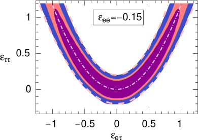
Figure 1: A 2-D section $(\mathrel{{\epsilon_{ee}}}=-0.15)$ of the allowed region of the NSI parameters (shaded). We assumed $\Delta m^{2}_{\odot}=0$ and $\theta_{13}=0$, and marginalized over $\theta$ and $\Delta m^{2}$. The dashed contours indicate our analytical predictions. See text for details.

Upon scanning the parameter space and marginalizing over $\Delta m^{2}$ and $\theta$ we obtain the three-dimensional allowed region in the space $(\mathrel{{\epsilon_{ee}}},\mathrel{{\epsilon_{e\tau}}},\mathrel{{\epsilon_{\tau\tau}}})$. As an illustration, in Fig. 1 we show a section of this region by the plane $\mathrel{{\epsilon_{ee}}}=-0.15$ (the choice motivated by the solar analysis in oursolar ). The $\chi^{2}$ minimum occurs at $\mathrel{{\epsilon_{e\tau}}}=0.07,\mathrel{{\epsilon_{\tau\tau}}}=0.01$; the value at the minimum, $\chi^{2}_{\rm min}=48.50$, is virtually the same as at the origin (no NSI), $\chi_{\rm orig}^{2}=48.57$. The shaded regions correspond, from the innermost contour, to $\chi^{2}-\chi^{2}_{\rm min}\leq$ 7.81, 11.35, and 18.80. They represent the 95%, 99%, and $3.6\sigma$ confidence levels (C.L.) for three degrees of freedom (d.o.f.). The last contour also corresponds to the 95% C.L. for 50 d.o.f.. For the purpose of hypothesis testing this means that a theory which gives NSI outside of this region should be rejected.

The dashed-dotted parabola illustrates the condition of zero eigenvalue, Eq. (6); the two outer curves give the predicted bound according to Eq. (5). For both, the agreement between the theory and numerical results is quite convincing. Moreover, we have verified that the agreement remains very good for $\mathrel{{\epsilon_{ee}}}$ in the range $-0.7<\mathrel{{\epsilon_{ee}}}<0.3$ inprep . For the case when only $\mathrel{{\epsilon_{e\tau}}}$ is non-zero we find the bounds $|\mathrel{{\epsilon_{e\tau}}}|<0.38$ at 99% C.L. and $|\mathrel{{\epsilon_{e\tau}}}|<0.5$ at $3.6\sigma$.

The extent of the allowed region along the parabola is beyond the scope of our analytical treatment. Indeed, since at high energy the leading NSI effect is canceled by construction, the fit quality is determined by subdominant NSI effects in all energy samples. Remarkably, these effects are rather small, especially for the inverted mass hierarchy, where the region $\chi^{2}-\chi^{2}_{\rm min}\leq 7.81$ extends up to $\mathrel{{\epsilon_{e\tau}}}=1$, as the Figure shows. The extent is somewhat smaller (to $\mathrel{{\epsilon_{e\tau}}}=\pm 0.6$) for the normal hierarchy inprep .

As mentioned, the symmetry of Fig. 1 with respect to $\mathrel{{\epsilon_{e\tau}}}\leftrightarrow-\mathrel{{\epsilon_{e\tau}}}$ follows from setting $\theta_{13}$ and $\Delta m_{\odot}^{2}$ to zero. We have checked that for $\theta_{13}\neq 0$ the region does indeed develop a small asymmetry inprep .

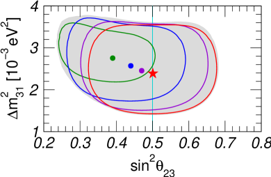
Figure 2: The effect of the NSI on the allowed region and best-fit values of the oscillation parameters; see text for details.

Finally, we notice that as the NSI point is moved along the parabola (6) away from the origin, the best-fit oscillation parameters change. This behavior is illustrated in Fig. 2. The four contours plotted are the sections of the five-dimensional allowed region in the space $(\Delta m^{2},\theta,\mathrel{{\epsilon_{ee}}},\mathrel{{\epsilon_{e\tau}}},\mathrel{{\epsilon_{\tau\tau}}})$ for the values: (i) $\mathrel{{\epsilon_{ee}}}=-0.15,\mathrel{{\epsilon_{e\tau}}}=0,\mathrel{{\epsilon_{\tau\tau}}}=0$; (ii) $\mathrel{{\epsilon_{ee}}}=-0.15,\mathrel{{\epsilon_{e\tau}}}=0.30,\mathrel{{\epsilon_{\tau\tau}}}=0.106$; (iii) $\mathrel{{\epsilon_{ee}}}=-0.15,\mathrel{{\epsilon_{e\tau}}}=0.60,\mathrel{{\epsilon_{\tau\tau}}}=0.424$; (iv) $\mathrel{{\epsilon_{ee}}}=-0.15,\mathrel{{\epsilon_{e\tau}}}=0.90,\mathrel{{\epsilon_{\tau\tau}}}=0.953$. The contours are drawn for $\Delta\chi^{2}=11.07$ with respect to the global minimum, marked by a star (this corresponds to 95% CL for 5 d.o.f.). The dots represent the best fit points obtained in each of the four cases above, when the NSI are assumed known. The figure confirms the trend predicted in Eq. (8): as the NSI increase the best-fit mixing angle becomes smaller, $\theta<\pi/4$, while the best-fit $\Delta m^{2}$ increases.

The shaded region in the background represents the result of marginalizing with respect to $\mathrel{{\epsilon_{e\tau}}}$ and $\mathrel{{\epsilon_{\tau\tau}}}$ (for $\mathrel{{\epsilon_{ee}}}=-0.15$). It was drawn for $\Delta\chi^{2}=11.83$, corresponding to 99.73% ($3\sigma$) C.L. for 2 d.o.f. While the best-fit point is nominally unchanged by the NSI, the shape of the $\chi^{2}$ function is significantly altered, so that small values of the mixing angle are now much less disfavored.

V Conclusion and implications

In conclusion, the three-flavor oscillation analysis exhibits qualitatively new features compared with the $\nu_{\mu}\leftrightarrow\nu_{\tau}$ studies. While giving no positive evidence for non-standard physics, the data do not exclude large NSI. The old bound $|\mathrel{{\epsilon_{\tau\tau}}}|<0.15$ at 99% C.L. is significantly relaxed by the addition of nonzero $\mathrel{{\epsilon_{e\tau}}}$: if $\mathrel{{\epsilon_{e\tau}}}$ and $\mathrel{{\epsilon_{\tau\tau}}}$ are varied simultaneously, even $\mathrel{{\epsilon_{\tau\tau}}}\sim 1$ is allowed. The effect is even more dramatic when one compares the bounds on the flavor-changing interactions: the bound $\mathrel{{\epsilon_{\mu\tau}}}<\mbox{a few}\times 10^{-2}$ Maltoni2001 does not extend to $\mathrel{{\epsilon_{e\tau}}}$, for which order one values are allowed. The bound $\mathrel{{\epsilon_{e\tau}}}<0.38$ at 99% C.L. – found for the case when the other epsilons vanish – is likewise new. We also stress that the effects of these large NSI are absolutely non-trivial. In particular, the best-fit values of the oscillation parameters shift to smaller angles and higher $\Delta m^{2}$. The physical mechanism behind this is well understood analytically.

These properties have important implications for other neutrino experiments. For example, the MINOS experiment will measure the mixing angle $\theta$ with good precision; assuming the true value $\theta=\pi/4$ one expects $\sin^{2}\theta>0.4$ at 99% C.L. MINOSreach . Given its baseline of only 735 km, MINOS will be almost free from matter effects and will therefore determine the vacuum value of $\theta$. Thus, it can look for the large NSI effects described here: a measurement of $\sin^{2}\theta>0.4$ and low $\Delta m^{2}$ would contribute to disfavor large NSI, while in the opposite case ($\sin^{2}\theta\sim 0.3$) one would have indications of non-standard physics.

Further tests can be performed at future experiments with longer baseline (a few $\times 10^{3}$ km) and sufficiently high energy, $E_{\nu}\sim 20-30$ GeV. These will be directly sensitive to the NSI matter effects and a discrepancy between them and MINOS could be a sign of NSI.

It is worth mentioning that, in principle, another signature of large NSI could be an unexpected number of neutral current events in a detector relative to the number of charged current events for a given oscillation scenario. This effect would be due to the modification of the detection neutral current cross section by large $\mathrel{{\epsilon_{e\tau}}}$ and $\mathrel{{\epsilon_{\tau\tau}}}$. Unfortunately, no firm prediction on the size of the effect can be made, since the effect additionally depends on the values of the axial couplings that do not enter the propagation Hamiltonian .

Finally, there are important implications for solar neutrinos. Indeed, $\mathrel{{\epsilon_{ee}}}$, $\mathrel{{\epsilon_{e\tau}}}$, and $\mathrel{{\epsilon_{\tau\tau}}}$ also enter the solar neutrino survival probability, and may alter the interpretation of the current data oursolar ; brazilians ; valencians . Our results here demonstrate that the LMA-0 solution, obtained with non-zero $\mathrel{{\epsilon_{e\tau}}}$ as in oursolar , is compatible with the atmospheric data. On the other hand, solar neutrinos, being sensitive to the phase of $\mathrel{{\epsilon_{e\tau}}}$, may rule out a sizable portion of the parameter space with $\mathrel{{\epsilon_{e\tau}}}<0$ oursolar ; inprep . This exclusion is impacted by the latest results from KamLAND KamLAND2004 and it would be very interesting to see the combined bound from the atmospheric, solar, and KamLAND data.