Universal Non-Oblique Corrections
in Higgsless Models and Beyond

Abstract:

Recently Barbieri, et al. have introduced a formalism to express the deviations of electroweak interactions from their standard model forms in “universal” theories, i.e. theories in which the corrections due to new physics can be expressed solely by modifications to the two-point correlation function of electroweak gauge currents of fermions. The parameters introduced by these authors are defined by the properties of the correlation functions at zero momentum, and differ from the quantities calculated by examining the on-shell properties of the electroweak gauge bosons. In this letter we discuss the relationship between the zero-momentum and on-shell parameters. In addition, we present the results of a calculation of these zero-momentum parameters in an arbitrary Higgsless model in which the low-energy $\rho$ parameter is one and which can be deconstructed to a linear chain of $SU(2)$ groups adjacent to a chain of $U(1)$ groups. Our results demonstrate the importance of the universal “non-oblique” corrections which are present and elucidate the relationships among various calculations of electroweak quantities in these models. Our expressions for these zero-momentum parameters depend only on the spectrum of heavy vector-boson masses; therefore, the minimum size of the deviations present in these models is related to the upper bound on the heavy vector-boson masses derived from unitarity. We find that these models are disfavored by precision electroweak data, independent of any assumptions about the background metric or the behavior of the bulk coupling.

1 Introduction

The standard electroweak model is in excellent agreement with the majority of experimental data. Despite this agreement, the agent of electroweak symmetry breaking remains elusive. Furthermore the one-doublet Higgs model, the simplest way to accommodate symmetry breaking, is unsatisfactory. These observations motivate the theoretical search for alternatives to the one-doublet Higgs model and the careful examination of precision electroweak data to motivate or constrain extensions to the standard model.

Recently, there have been interesting work on both of these fronts. On the theoretical side, “Higgsless” models of electroweak symmetry breaking have been proposed [1]. Based on five-dimensional gauge theories compactified on an interval, these models achieve unitarity of electroweak boson self-interactions through the exchange of a tower of massive vector bosons [2, 3, 4], rather than the exchange of a scalar Higgs boson [5]. Motivated by gauge/gravity duality [6, 7, 8, 9], models of this kind may be viewed as “dual” to more conventional models of dynamical symmetry breaking [10, 11] such as “walking techicolor” [12, 13, 14, 15, 16, 17].

On the phenomenological side, Barbieri et al. [18] have introduced a formalism to express the deviations of electroweak interactions from their standard model forms in “universal” theories, i.e. theories in which the corrections due to new physics can be expressed solely by modifications to the two-point correlation function of electroweak gauge currents of fermions. The parameters introduced by these authors are defined by the properties of the correlation functions at zero momentum, and differ from the more familiar quantities calculated by examining the on-shell properties of the electroweak gauge bosons.

In this letter we discuss the relationship between the zero-momentum and on-shell parameters. In addition, we present the results of a calculation of these zero-momentum parameters in a general class of Higgsless models in which the low-energy rho parameter is one and which can be deconstructed [19, 20] to a linear chain of $SU(2)$ groups adjacent to a chain of $U(1)$ groups. The details of the calculation of the zero-momentum parameters in deconstructed higgsless models, which extend the results of [21], will be presented in a forthcoming publication [22].

Our results demonstrate the importance of the universal “non-oblique” corrections which are present in these models and elucidate the relationships among various calculations of electroweak quantities in these models [23, 24, 25, 26, 27, 28, 29, 18, 30, 31]. Our expressions for these zero-momentum parameters depend only on the spectrum of heavy vector-boson masses; therefore, the minimum size of the deviations present in these models is related to the upper bound on the heavy vector-boson masses derived from unitarity. We find that these models are disfavored by precision electroweak data, independent of any assumptions about the background metric or the behavior of the bulk coupling.

2 Parameterizing Deviations from the Standard Model

Barbieri et al. [18] choose parameters to describe four-fermion electroweak processes using the transverse gauge-boson polarization amplitudes. Formally, all such processes can be summarized in momentum space (at tree-level in the electroweak interactions, having integrated out all heavy states, and ignoring external fermion masses) by the charged current Lagrangian

$${\cal L}_{cc}={1\over 2}\left[\Pi_{W^{+}W^{-}}(Q^{2})\right]^{-1}J^{\mu}_{+}J_{-\mu}~{},$$ (1)

and the neutral current Lagrangian

$${\cal L}_{nc}={1\over 2}\left(\begin{array}[]{cc}J_{3\mu}&J_{B\mu}\end{array}\right)\left[\begin{array}[]{cc}{\Pi}_{W^{3}W^{3}}(Q^{2})&{\Pi}_{W^{3}B}(Q^{2})\\ {\Pi}_{W^{3}B}(Q^{2})&{\Pi}_{BB}(Q^{2})\end{array}\right]^{-1}\left(\begin{array}[]{c}J^{\mu}_{3}\\ J_{B}^{\mu}\end{array}\right)~{},$$ (2)

where the $\vec{J}^{\mu}$ and $J_{B}^{\mu}$ are the weak isospin and hypercharge fermion currents respectively. All two-point correlation functions of fermionic currents – and therefore all four-fermion scattering amplitudes at tree-level – can be read off from the appropriate element(s) of the inverse gauge-boson polarization matrix. Throughout this paper, in order to be consistent with [21], we use $Q^{2}=-q^{2}$ to denote the Euclidean momentum-squared.

Barbieri et al. proceed by defining the (approximate) electroweak couplings

$${1\over g^{2}}\equiv\left[d\Pi_{W^{+}W^{-}}(Q^{2})\over d(-Q^{2})\right]_{Q^{2}=0}\ \ \ \ ,\ \ \ {1\over{g^{\prime}}^{2}}\equiv\left[{d\Pi_{BB}(Q^{2})\over d(-Q^{2})}\right]_{Q^{2}=0}~{},$$ (3)

and the electroweak scale

$$v^{2}\equiv-4\,\Pi_{W^{+}W^{-}}(0)=(\sqrt{2}G_{F})^{-1}\approx(246\,{\rm GeV})^{2}~{}.$$ (4)

In terms of the polarization functions and these constants, the authors of [18] define the parameters

$$\hat{S} \equiv g^{2}\left[{d\Pi_{W^{3}B}(Q^{2})\over d(-Q^{2})}\right]_{Q^{2}=0}~{},$$ (5)

$$\hat{T} \equiv {g^{2}\over M^{2}_{W}}\left(\Pi_{W^{3}W^{3}}(0)-\Pi_{W^{+}W^{-}}(0)\right)~{},$$ (6)

$$W \equiv {g^{2}M^{2}_{W}\over 2}\left[{d^{2}\Pi_{W^{3}W^{3}}(Q^{2})\over d(-Q^{2})^{2}}\right]_{Q^{2}=0}~{},$$ (7)

$$Y \equiv {{g^{\prime}}^{2}M^{2}_{W}\over 2}\left[{d^{2}\Pi_{BB}(Q^{2})\over d(-Q^{2})^{2}}\right]_{Q^{2}=0}~{}.$$ (8)

In any non-standard electroweak model in which all of the relevant effects occur only in the correlation function of fermionic electroweak gauge currents, the values of these four parameters [18] summarize the leading deviations in all four-fermion processes from the standard model predictions. The quantities $\hat{U}$, $\hat{V}$ and $X$ defined in [18] describe higher-order effects.

While the parameters of eqns. (5)-(8) succinctly summarize the deviations from the standard model in any universal extension, they do not correspond simply to the on-shell properties of the $Z$ or $W$ bosons, the properties most easily calculated when considering models with extra gauge bosons, for example. Instead, it is useful to characterize the matrix element for four-fermion neutral weak current processes by

$$-{\cal M}_{NC}=e^{2}{{\cal Q}{\cal Q}^{\prime}\over Q^{2}} + \frac{\displaystyle{(I_{3}-s^{2}{\cal Q})(I^{\prime}_{3}-s^{2}{\cal Q}^{\prime})}}{\displaystyle{\left({s^{2}c^{2}\over e^{2}}-{S\over 16\pi}\right)Q^{2}+{1\over 4\sqrt{2}G_{F}}\left(1-\alpha T+{\alpha\delta\over 4s^{2}c^{2}}\right)}}$$

$$+ \sqrt{2}G_{F}\,{\alpha\delta\over s^{2}c^{2}}\,I_{3}I^{\prime}_{3}+4\sqrt{2}G_{F}\left(\Delta\rho-\alpha T\right)({\cal Q}-I_{3})({\cal Q}^{\prime}-I_{3}^{\prime})~{},$$

and the matrix element for charged currents by

$$-{\cal M}_{\rm CC}=\frac{\displaystyle{(I_{+}I^{\prime}_{-}+I_{-}I^{\prime}_{+})/2}}{\displaystyle{\left(\frac{\displaystyle{s^{2}}}{\displaystyle{e^{2}}}-\frac{\displaystyle{S}}{\displaystyle{16\pi}}\right)Q^{2}+{1\over 4\sqrt{2}G_{F}}\left(1+{\alpha\delta\over 4s^{2}c^{2}}\right)}}+\sqrt{2}G_{F}\,{\alpha\delta\over s^{2}c^{2}}\,{(I_{+}I^{\prime}_{-}+I_{-}I^{\prime}_{+})\over 2}~{}.$$ (10)

Here $I^{(\prime)}_{a}$ and ${\cal Q}^{(\prime)}$ are weak isospin and charge of the corresponding fermion, $\alpha=e^{2}/4\pi$, $G_{F}$ is the usual Fermi constant, and the weak mixing angle (as defined by the on-shell $Z$ coupling) is denoted by $s^{2}$ ($c^{2}\equiv 1-s^{2}$).

Some comments about the amplitudes in eqns. (2) and (10) are in order. First, $\Delta\rho$ corresponds to the deviation from unity of the ratio of the strengths of low-energy isotriplet weak neutral-current scattering and charged-current scattering. $S$ and $T$ are the familiar oblique electroweak parameters [33, 34, 35], as determined by examining the on-shell properties of the $Z$ and $W$ bosons. Finally, the contact interactions proportional to $\alpha\delta$ and ($\Delta\rho-\alpha T$) correspond to “universal non-oblique” corrections. They are “universal” in the sense that they can be seen to arise from effective operators proportional to $\vec{J}^{2}_{\mu}$ and $J^{2}_{B}$, and therefore modify the correlation function of fermionic electroweak currents. They are “non-oblique” in the sense that they do not correspond to deviations of the on-shell $W$- and $Z$-boson propagators. As shown in [21], such universal non-oblique effects occur in a variety of Higgsless models of electroweak symmetry breaking – and the presence of such effects need not lead to deviations in the low-energy $\rho$ parameter from one.

Relating the parameters $\alpha S$, $\alpha T$, $\alpha\delta$, and $\Delta\rho$ to $\hat{S}$, $\hat{T}$, $W$, and $Y$ is straightforward: inverting the charged-current matrix element of eqn. (10) yields $\Pi_{W^{+}W^{-}}(Q^{2})$, and finding the inverse of the $2\times 2$ matrix in the space of currents $(J_{3\mu},J_{B\mu})$, defined implicitly by eqn. (2), yields the neutral-current matrix ${\bf\Pi}(Q^{2})$. In the limit where all corrections to the standard model go to zero, one finds

$$\Pi^{SM}_{W^{+}W^{-}}(Q^{2})=-{s^{2}\over e^{2}}\left[Q^{2}+{e^{2}\over 4\sqrt{2}s^{2}G_{F}}\right]~{},$$ (11)

and

$${\bf\Pi}^{SM}(Q^{2})=-{1\over e^{2}}\,\left(\begin{array}[]{cc}s^{2}Q^{2}+c^{2}s^{2}\mu^{2}_{Z}&-s^{2}c^{2}\mu^{2}_{Z}\\ -s^{2}c^{2}\mu^{2}_{Z}&c^{2}Q^{2}+c^{2}s^{2}\mu^{2}_{Z}\end{array}\right)~{},$$ (12)

where we have defined

$$\mu^{2}_{Z}\equiv{e^{2}\over 4\sqrt{2}G_{F}s^{2}c^{2}}~{},$$ (13)

for convenience. From these lowest-order expressions, we immediately find from eqn. (3)

$${1\over g^{2}}\approx{e^{2}\over s^{2}}\ \ \ \ ,\ \ \ {1\over{g^{\prime}}^{2}}\approx{e^{2}\over c^{2}}~{},$$ (14)

as expected.

Calculating ${\bf\Pi}(Q^{2})$ to leading order in the deviations from the standard model, one finds the relations

$$\hat{S} = {1\over 4s^{2}}\left(\alpha S+4c^{2}(\Delta\rho-\alpha T)+{\alpha\delta\over c^{2}}\right)$$ (15)

$$\hat{T} = \Delta\rho$$ (16)

$$W = {\alpha\delta\over 4s^{2}c^{2}}$$ (17)

$$Y = {c^{2}\over s^{2}}(\Delta\rho-\alpha T)~{}.$$ (18)

Inverting these relationships, we find

$$\alpha S = 4s^{2}(\hat{S}-Y-W)$$ (19)

$$\alpha T = \hat{T}-{s^{2}\over c^{2}}Y$$ (20)

$$\alpha\delta = 4s^{2}c^{2}W$$ (21)

$$\Delta\rho = \hat{T}~{}.$$ (22)

In the absence of any universal non-oblique corrections, $W=Y=0$, one finds the relations

$$\hat{S}={\alpha S\over 4s^{2}}\ \ \ ,\ \ \hat{T}=\alpha T~{},$$ (23)

given in [18].

Note that it is the non-oblique universal corrections described by $Y$ that mark the difference between $\Delta\rho$ and $T$. In a model with $Y=0$ we have $\Delta\rho=\hat{T}=\alpha T$, so that the case of greatest phenomenological interest with $\Delta\rho=0$ would also have vanishing $\hat{T}$ and $T$. However, in a model with non-zero $Y$, focusing on the case with $\Delta\rho=0$ ensures that $\hat{T}$ vanishes, but still allows $\alpha T$ to be non-zero.

3 Application to Higgsless Models

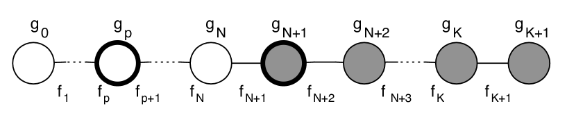
Figure 1: Moose diagram for the class of models discussed in this letter. All $N+1$ of the $SU(2)$ gauge groups are shown as open circles; all $M+1$ of the $U(1)$ gauge groups, as shaded circles; and $K=N+M$. The fermions couple to gauge gauge groups $p$ and $N+1$. The values of the gauge couplings $g_{i}$ and decay constants $f_{i}$ are arbitrary.

We may now apply these results to Higgsless models. Using deconstruction [19, 20] , the most general Higgsless model in which the low-energy $\rho$ parameter is one [22] is shown diagrammatically in Fig. 1 (in “moose notation” [37, 19]). These models incorporate an $SU(2)^{N+1}\times U(1)^{M+1}$ gauge group, and $N+1$ nonlinear $(SU(2)\times SU(2))/SU(2)$ sigma models adjacent to $M$ $(U(1)\times U(1))/U(1)$ sigma models in which the global symmetry groups in adjacent sigma models are identified with the corresponding factors of the gauge group. The Lagrangian for this model at $O(p^{2})$ is given by

$${\cal L}_{2}=\frac{1}{4}\sum_{j=1}^{N+M+1}f_{j}^{2}\mbox{tr}\left((D_{\mu}U_{j})^{\dagger}(D^{\mu}U_{j})\right)-\sum_{j=0}^{N+M+1}\frac{\displaystyle{1}}{\displaystyle{2g_{j}^{2}}}\mbox{tr}\left(F^{j}_{\mu\nu}F^{j\mu\nu}\right),$$ (24)

with

$$D_{\mu}U_{j}=\partial_{\mu}U_{j}-iA^{j-1}_{\mu}U_{j}+iU_{j}A^{j}_{\mu},$$ (25)

where all gauge fields $A^{j}_{\mu}$ $(j=0,1,2,\cdots,N+M+1)$ are dynamical. The first $N+1$ gauge fields ($j=0,1,\ldots,N$) correspond to $SU(2)$ gauge groups; the other $M+1$ gauge fields ($j=N+1,N+2,\ldots,N+M+1$) correspond to $U(1)$ gauge groups. The symmetry breaking between the $A^{N}_{\mu}$ and $A^{N+1}_{\mu}$ follows an $SU(2)_{L}\times SU(2)_{R}/SU(2)_{V}$ symmetry breaking pattern with the $U(1)$ embedded as the $T_{3}$-generator of $SU(2)_{R}$.

The fermions in this model take their weak interactions from the $SU(2)$ group at $j=p$ and their hypercharge interactions from the $U(1)$ group with $j=N+1$, at the interface between the $SU(2)$ and $U(1)$ groups The neutral current couplings to the fermions are thus written as

$$J^{\mu}_{3}A^{p}_{\mu}+J^{\mu}_{B}A^{N+1}_{\mu}~{},$$ (26)

while the charged current couplings arise from

$${1\over\sqrt{2}}J^{\mu}_{\pm}A^{p\mp}_{\mu}~{}.$$ (27)

Generalizing the calculations of [21] one may calculate the polarization functions $\Pi_{W^{+}W^{-}}(Q^{2})$ and ${\bf\Pi}(Q^{2})$ at tree-level [22]. We find that

$$\Pi_{W^{+}W^{-}}(Q^{2})=\Pi_{W^{3}W^{3}}(Q^{2})~{},$$ (28)

and therefore the parameter $\hat{T}$, as well as the higher-order parameters $\hat{U}$ and $\hat{V}$ [18], vanishes identically in any of these models.

The results for the non-zero parameters are most conveniently expressed in terms of the eigenvalues of various sub-matrices of the full neutral vector-boson mass-squared matrix. Generalizing the usual mathematical notation for “open” and “closed” intervals, we may denote the neutral-boson mass matrix $M^{2}_{Z}$ as $M^{2}_{[0,N+M+1]}$ — i.e. it is the mass matrix for the entire moose running from site $0$ to site $N+M+1$ including the gauge couplings of both endpoint groups. Analogously, the charged-boson mass matrix $M^{2}_{W}$ is $M^{2}_{[0,N+1)}$ — it is the mass matrix for the moose running from site $0$ to link $N+1$, but not including the gauge couping at site $N+1$. Using this notation, we define sub-matrices:

$${\cal M}^{2}_{p} = M^{2}_{[0,p)}$$ (29)

$${\cal M}^{2}_{r} = M^{2}_{(p,N+1)}$$ (30)

$${\cal M}^{2}_{q} = M^{2}_{(N+1,N+M+1]}$$ (31)

of the neutral gauge-boson mass-squared matrix. They fit together inside $M_{Z}^{2}$ as follows:

$${\tiny M_{Z}^{2}=\left(\begin{array}[]{cc|c|ccc|c|cc}&{\cal M}_{p}^{2}&&&&&&&\\ &&-g_{p-1}g_{p}f_{p}^{2}/4&&&&&&\\ \hline\cr&-g_{p-1}g_{p}f_{p+1}^{2}/4&g_{p}^{2}(f_{p}^{2}+f_{p+1}^{2})/4&-g_{p}g_{p+1}f_{p+1}^{2}/4&&&&&\\ \hline\cr&&-g_{p}g_{p+1}f_{p+1}^{2}/4&&&&&&\\ &&&&{\cal M}_{r}^{2}&&&&\\ &&&&&&-g_{N}g_{N+1}f_{N+1}^{2}/4&&\\ \hline\cr&&&&&-g_{N}g_{N+1}f_{N+2}^{2}/4&g_{N+1}^{2}(f_{N+1}^{2}+f_{N+2}^{2})/4&-g_{N+1}g_{N+2}f_{N+2}^{2}/4&\\ \hline\cr&&&&&&-g_{N+1}g_{N+1}f_{N+2}^{2}/4&&\\ &&&&&&&{\cal{M}}_{q}^{2}\\ \end{array}\right).}$$ (32)

In the phenomenologically relevant limit, in which the only light vector bosons correspond to the usual $\gamma$, $W$, and $Z$, the eigenvalues of these matrices (${\mathsf{m}}^{2}_{\hat{p},\hat{r},\hat{q}}$ respectively) must be large, ${\mathsf{m}}^{2}_{\hat{p},\hat{r},\hat{q}}\gg M^{2}_{W,Z}$ [22]. It is therefore appropriate to expand in inverse powers of the large mass eigenvalues. We define

$$\Sigma_{Z}=\sum_{\hat{z}=1}^{N+M}{1\over{\mathsf{m}}^{2}_{\hat{z}}}\ \ \ \ ,\ \ \ \Sigma_{W}=\sum_{\hat{w}=1}^{N}{1\over{\mathsf{m}}^{2}_{\hat{w}}}~{},$$ (33)

where the sums run only over the heavy eigenstates (i.e. they exclude the light $W$, light $Z$ and photon), and

$$\Sigma_{p}=\sum_{\hat{p}=0}^{p-1}{1\over{\mathsf{m}}^{2}_{\hat{p}}}\ \ ,\ \ \Sigma_{r}=\sum_{\hat{r}=p+1}^{N}{1\over{\mathsf{m}}^{2}_{\hat{r}}}\ \ ,\ \ \Sigma_{q}=\sum_{\hat{q}=N+2}^{N+M+1}{1\over{\mathsf{m}}^{2}_{\hat{q}}}~{}.$$ (34)

where the sums run over all of the submatrix eigenvalues.

We can write the electroweak parameters in terms of these sums over eigenvalues. The on-shell parameters (recalling that $\Delta\rho\equiv 0$) take the form [22]

$$\alpha S = 4s^{2}M^{2}_{W}(\Sigma_{Z}-\Sigma_{p}-\Sigma_{q})$$ (35)

$$\alpha T = s^{2}M^{2}_{Z}(\Sigma_{Z}-\Sigma_{W}-\Sigma_{q})$$ (36)

$${\alpha\delta\over c^{2}} = -4s^{2}M^{2}_{W}(\Sigma_{W}-\Sigma_{p}-\Sigma_{r})~{}.$$ (37)

Clearly it is possible for $S$ to be small or even negative. In the case where the fermions couple to the $SU(2)$ group at the left end of the moose (i.e., $p=0$), these reduce to the expressions found in [21]: $\Sigma_{p}=0$, our $\Sigma_{q}$ is equivalent to $\Sigma_{M}$ in the earlier paper, and $M_{W}^{2}$ may be used in place of $c^{2}M_{Z}^{2}$ to leading order in these expressions.

Using the relations (15) - (18) we can write the zero-momentum parameters as

$$\hat{S} = M^{2}_{W}\,\Sigma_{r}>0$$ (38)

$$\hat{T} = 0$$ (39)

$$W = -M^{2}_{W}(\Sigma_{W}-\Sigma_{p}-\Sigma_{r})$$ (40)

$$Y = -M^{2}_{W}(\Sigma_{Z}-\Sigma_{W}-\Sigma_{q})~{},$$ (41)

to leading non-trivial order. As noted, the parameter $\hat{S}$ is always strictly positive, in agreement with the arguments presented in [25]. Re-expressing $\hat{S}$ in terms of the on-shell parameters (setting $\Delta\rho=0$ as appropriate in this class of models) we see that

$$\hat{S}={\alpha\over 4s^{2}}\left(S-4c^{2}T+{\delta\over c^{2}}\right)=M^{2}_{W}\Sigma_{r}>0~{},$$ (42)

generalizing the result of [21]. Furthermore, we see that, due to the presence of non-oblique universal corrections the positivity of $\hat{S}$ is not in contradiction with small, or even negative, values of $\alpha S$ [28, 29].

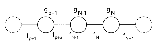
Figure 2: Moose diagram whose vector boson mass matrix corresponds to ${\cal M}^{2}_{r}$, which runs from link $p+1$ to link $N+1$ of the original moose in Fig. 1. The endpoints are ungauged and the dashed circles indicate global groups. The $F$-constant of the physical pions of this model is $v$.

In any unitary theory [2, 3], we expect the mass of the lightest additional vector to be less than $\sqrt{8\pi}v$ ($v\approx 246$ GeV), the scale at which $WW$ spin-0 isospin-0 elastic scattering would violate unitarity in the standard model in the absence of a higgs boson [38, 39, 40, 41, 42, 43]. In the case that $M^{2}_{W}\,\Sigma_{Z,W,p,q,r}\ll 1$, the Goldstone boson corresponding to the longitudinal $W$ is approximately the pion of the model shown in Fig. 2 [22]. Unitarity, therefore, requires that the lightest eigenvalue of the matrix ${\cal M}^{2}_{r}$ must be of order $8\pi v^{2}$ or lighter. Evaluating eqn. (42) then reveals $S-4c^{2}T+\delta/c^{2}$ to be of order one-half or larger, generalizing the result of [21]. The corresponding value of $\hat{S}$ this large is disfavored by precision electroweak data [18].

4 Summary

In this letter about universal theories, we have related the parameters ($\hat{S}$, $\hat{T}$, $W$, $Y$,) introduced by Barbieri et al. to describe zero-momentum deviations of the electroweak interactions from their standard model forms to the parameters ($S$, $T$, $\delta$, $\Delta\rho$) calculated in terms of the on-shell properties of the $W$ and $Z$ bosons. We have presented the results of a calculation [22] of these parameters in the most general Higgsless model in which the low-energy $\rho$ parameter is one. Our results demonstrate the importance of the universal non-oblique corrections which are generally present in these models. These results also elucidate the relationship between the various calculations of precision electroweak parameters in Higgsless models.

Specifically, we find $\hat{S}=(\alpha/4s^{2})(S-4c^{2}T+\delta/c^{2})>0$ which agrees with and extends previous findings [21, 18, 25]. Moreover, we find that unitarity considerations constrain $4s^{2}\hat{S}/\alpha$ to be greater than or of order one-half in these models, a value so large as to be severely disfavored [18] by precision electroweak data.

The details of the calculations of the various correlation functions in Higgsless models, the generalization to models with $\Delta\rho\neq 0$, and the connection to an expansion in large “bulk” coupling [44], will be presented in [22].

5 Note Added in Proof

After the submission of this manuscript, a new class of Higgsless models with delocalized fermions has been proposed [45, 46], and it has been shown that the delocalization of the fermions can be adjusted to minimize the deviations of the electroweak interactions from their Standard Model forms. The techniques discussed here and in [22] must be extended to accommodate fermion delocalization, and this topic is under current investigation.

- [1] C. Csaki, C. Grojean, H. Murayama, L. Pilo, and J. Terning, Gauge theories on an interval: Unitarity without a higgs, hep-ph/0305237.
- [2] R. Sekhar Chivukula, D. A. Dicus, and H.-J. He, Unitarity of compactified five dimensional yang-mills theory, Phys. Lett. B525 (2002) 175–182, [hep-ph/0111016].
- [3] R. S. Chivukula and H.-J. He, Unitarity of deconstructed five-dimensional yang-mills theory, Phys. Lett. B532 (2002) 121–128, [hep-ph/0201164].
- [4] R. S. Chivukula, D. A. Dicus, H.-J. He, and S. Nandi, Unitarity of the higher dimensional standard model, Phys. Lett. B562 (2003) 109–117, [hep-ph/0302263].
- [5] P. W. Higgs, Broken symmetries, massless particles and gauge fields, Phys. Lett. 12 (1964) 132–133.
- [6] J. M. Maldacena, The large n limit of superconformal field theories and supergravity, Adv. Theor. Math. Phys. 2 (1998) 231–252, [hep-th/9711200].
- [7] S. S. Gubser, I. R. Klebanov, and A. M. Polyakov, Gauge theory correlators from non-critical string theory, Phys. Lett. B428 (1998) 105–114, [hep-th/9802109].
- [8] E. Witten, Anti-de sitter space and holography, Adv. Theor. Math. Phys. 2 (1998) 253–291, [hep-th/9802150].
- [9] O. Aharony, S. S. Gubser, J. M. Maldacena, H. Ooguri, and Y. Oz, Large n field theories, string theory and gravity, Phys. Rept. 323 (2000) 183–386, [hep-th/9905111].
- [10] S. Weinberg, Implications of dynamical symmetry breaking: An addendum, Phys. Rev. D19 (1979) 1277–1280.
- [11] L. Susskind, Dynamics of spontaneous symmetry breaking in the weinberg- salam theory, Phys. Rev. D20 (1979) 2619–2625.
- [12] B. Holdom, Raising the sideways scale, Phys. Rev. D24 (1981) 1441.
- [13] B. Holdom, Techniodor, Phys. Lett. B150 (1985) 301.
- [14] K. Yamawaki, M. Bando, and K.-i. Matumoto, Scale invariant technicolor model and a technidilaton, Phys. Rev. Lett. 56 (1986) 1335.
- [15] T. W. Appelquist, D. Karabali, and L. C. R. Wijewardhana, Chiral hierarchies and the flavor changing neutral current problem in technicolor, Phys. Rev. Lett. 57 (1986) 957.
- [16] T. Appelquist and L. C. R. Wijewardhana, Chiral hierarchies and chiral perturbations in technicolor, Phys. Rev. D35 (1987) 774.
- [17] T. Appelquist and L. C. R. Wijewardhana, Chiral hierarchies from slowly running couplings in technicolor theories, Phys. Rev. D36 (1987) 568.
- [18] R. Barbieri, A. Pomarol, R. Rattazzi, and A. Strumia, Electroweak symmetry breaking after lep1 and lep2, hep-ph/0405040.
- [19] N. Arkani-Hamed, A. G. Cohen, and H. Georgi, (de)constructing dimensions, Phys. Rev. Lett. 86 (2001) 4757–4761, [hep-th/0104005].
- [20] C. T. Hill, S. Pokorski, and J. Wang, Gauge invariant effective lagrangian for kaluza-klein modes, Phys. Rev. D64 (2001) 105005, [hep-th/0104035].
- [21] R. S. Chivukula, E. H. Simmons, H.-J. He, M. Kurachi, and M. Tanabashi, The structure of corrections to electroweak interactions in higgsless models, hep-ph/0406077.
- [22] R. S. Chivukula, E. H. Simmons, H.-J. He, M. Kurachi, and M. Tanabashi, “Electroweak corrections and unitarity in linear moose models,” hep-ph/0410154.
- [23] C. Csaki, C. Grojean, L. Pilo, and J. Terning, Towards a realistic model of higgsless electroweak symmetry breaking, Phys. Rev. Lett. 92 (2004) 101802, [hep-ph/0308038].
- [24] Y. Nomura, Higgsless theory of electroweak symmetry breaking from warped space, JHEP 11 (2003) 050, [hep-ph/0309189].
- [25] R. Barbieri, A. Pomarol, and R. Rattazzi, Weakly coupled higgsless theories and precision electroweak tests, hep-ph/0310285.
- [26] H. Davoudiasl, J. L. Hewett, B. Lillie, and T. G. Rizzo, Higgsless electroweak symmetry breaking in warped backgrounds: Constraints and signatures, hep-ph/0312193.
- [27] G. Burdman and Y. Nomura, Holographic theories of electroweak symmetry breaking without a higgs boson, hep-ph/0312247.
- [28] G. Cacciapaglia, C. Csaki, C. Grojean, and J. Terning, Oblique corrections from higgsless models in warped space, hep-ph/0401160.
- [29] H. Davoudiasl, J. L. Hewett, B. Lillie, and T. G. Rizzo, Warped higgsless models with ir-brane kinetic terms, JHEP 05 (2004) 015, [hep-ph/0403300].
- [30] N. Evans and P. Membry, Higgless w unitarity from decoupling deconstruction, hep-ph/0406285.
- [31] M. Perelstein, Gauge-assisted technicolor?, hep-ph/0408072.
- [32] R. S. Chivukula and H. Georgi, Phenomenology of composite technicolor standard models, Phys. Rev. D36 (1987) 2102.
- [33] M. E. Peskin and T. Takeuchi, Estimation of oblique electroweak corrections, Phys. Rev. D46 (1992) 381–409.
- [34] G. Altarelli and R. Barbieri, Vacuum polarization effects of new physics on electroweak processes, Phys. Lett. B253 (1991) 161–167.
- [35] G. Altarelli, R. Barbieri, and S. Jadach, Toward a model independent analysis of electroweak data, Nucl. Phys. B369 (1992) 3–32.
- [36] A. Strumia, Bounds on kaluza-klein excitations of the sm vector bosons from electroweak tests, Phys. Lett. B466 (1999) 107–114, [hep-ph/9906266].
- [37] H. Georgi, A tool kit for builders of composite models, Nucl. Phys. B266 (1986) 274.
- [38] D. A. Dicus and V. S. Mathur, Upper bounds on the values of masses in unified gauge theories, Phys. Rev. D7 (1973) 3111–3114.
- [39] J. M. Cornwall, D. N. Levin, and G. Tiktopoulos, Uniqueness of spontaneously broken gauge theories, Phys. Rev. Lett. 30 (1973) 1268–1270.
- [40] J. M. Cornwall, D. N. Levin, and G. Tiktopoulos, Derivation of gauge invariance from high-energy unitarity bounds on the s - matrix, Phys. Rev. D10 (1974) 1145.
- [41] B. W. Lee, C. Quigg, and H. B. Thacker, The strength of weak interactions at very high-energies and the higgs boson mass, Phys. Rev. Lett. 38 (1977) 883.
- [42] B. W. Lee, C. Quigg, and H. B. Thacker, Weak interactions at very high-energies: The role of the higgs boson mass, Phys. Rev. D16 (1977) 1519.
- [43] M. J. G. Veltman, Second threshold in weak interactions, Acta Phys. Polon. B8 (1977) 475.
- [44] H. Georgi, Fun with higgsless theories, hep-ph/0408067.
- [45] G. Cacciapaglia, C. Csaki, C. Grojean and J. Terning, “Curing the ills of Higgsless models: The S parameter and unitarity,” hep-ph/0409126.
- [46] R. Foadi, S. Gopalakrishna and C. Schmidt, “Effects of fermion localization in Higgsless theories and electroweak constraints,” hep-ph/0409266.