A Model for the Twist-3 Wave Function of the Pion and Its Contribution to the Pion Form Factor

Abstract

A model for the twist-3 wave function $\psi_{p}(x,\mathbf{k_{\perp}})$ of the pion has been constructed based on the moment calculation by applying the QCD sum rules, whose distribution amplitude has a better end-point behavior than that of the asymptotic one. With this model wave function, the twist-3 contributions including both the usual helicity components ($\lambda_{1}+\lambda_{2}=0$) and the higher helicity components ($\lambda_{1}+\lambda_{2}=\pm 1$) to the pion form factor have been studied within the modified pQCD approach. Our results show that the twist-3 contribution drops fast and it becomes less than the twist-2 contribution at $Q^{2}\sim 10GeV^{2}$. The higher helicity components in the twist-3 wave function will give an extra suppression to the pion form factor. The model dependence of the twist-3 contribution to the pion form factor has been studied by comparing four different models. When all the power contributions, which include higher order in $\alpha_{s}$, higher helicities, higher twists in DA and etc., have been taken into account, it is expected that the hard contributions will fit the present experimental data well at the energy region where pQCD is applicable.

PACS numbers: 13.40.Gp, 12.38.Bx, 11.55.Hx

I Introduction

The most challenging problems for applying the perturbative QCD (pQCD) to exclusive processes have long been discussed and analyzed in many papers, such as the pQCD applicability to the exclusive processes at experimentally accessible energy region due to the end-point singularity; to estimate the contributions from power corrections, which includes higher order in $\alpha_{s}$, higher helicities, higher twists in distribution amplitude (DA), higher Fock states and etc.; to estimate the uncertainties from perturbatively incalculable DAs.

The pion form factor can be obtained through the definition

$$\langle\pi(p^{\prime})|J_{\mu}|\pi(p)\rangle=(p+p^{\prime})_{\mu}F_{\pi}(Q^{2}),$$ (1)

where $J_{\mu}=\sum_{i}e_{i}\bar{q}_{i}\gamma_{\mu}q_{i}$, with the quark flavor $i$ and the relevant electric charge $e_{i}$, is the vector current. The momentum transfer $q^{2}=-Q^{2}=(p-p^{\prime})^{2}$ is restricted in the space-like region. The pQCD applicability to the pion form factor at the experimentally accessible energy region has been raised by Ref.isgur and attracted much attention for many years. In the modified pQCD approach that is proposed in Ref.lis , i.e. the transverse momentum dependence ($k_{T}$ dependence) as well as the Sudakov corrections are taken into account in the calculations, we have the following factorization formulalis ; pi2pi ; jps ; cchm ,

$$F_{\pi}(Q^{2})=\sum_{n,m}\int[dx_{i}d{\bf k}_{\perp i}]_{n}[dy_{j}d{\bf l}_{\perp j}]_{m}\psi_{n}(x_{i},{\bf k}_{\perp i};\mu_{f})T_{nm}(x_{i},{\bf k}_{\perp i};y_{j},{\bf l}_{\perp j};\mu_{f})\psi_{m}(y_{j},{\bf l}_{\perp j};\mu_{f}),$$ (2)

where $[dx_{i}d\mathbf{k}_{i}]_{n}$ is the relativistic measure within the $n$-particle sector, $n,\ m$ extend over the low momentum states only and $T_{nm}$ are the partonic matrix elements of the effective current operator. Here the helicity states of the pion are implied in both sides. The dependence on the scale separating low (non-perturbative) and high momenta (perturbative) is indicated by $\mu_{f}$. For the valence quark state of the pion, its light cone (LC) wave functions are defined in terms of the bilocal operator matrix elementBenekeFeldmann ,

$$\langle\pi(p)|\bar{q}_{\beta}(z)q_{\alpha}|0\rangle = \frac{if_{\pi}}{4}\int_{0}^{1}dx\int d^{2}{\bf k}_{\bot}e^{i(xp\cdot z-{\bf k}_{\bot}\cdot{\bf z}_{\bot})}$$ (3)

$$\times \left\{/\!\!\!p\gamma_{5}\psi_{\pi}(x,{\bf k}_{\bot})-\mu_{\pi}\gamma_{5}\left(\psi_{p}(x,{\bf k}_{\bot})-\sigma_{\mu\nu}p^{\mu}z^{\nu}\frac{\psi_{\sigma}(x,{\bf k}_{\bot})}{6}\right)\right\}_{\alpha\beta},$$

where $\mu_{\pi}=m_{\pi}^{2}/(m_{u}+m_{d})$ and $f_{\pi}$ is the pion decay constant, whose experimental value is $130.7\pm 0.1\pm 0.36MeV$pdg . $\psi_{\pi}(x,\mathbf{k_{\perp}})$ is the leading twist (twist-2) wave function, $\psi_{p}(x,\mathbf{k_{\perp}})$ and $\psi_{\sigma}(x,\mathbf{k_{\perp}})$ are sub-leading twist (twist-3) wave functions that correspond to the pseudo-scalar structure and the pseudo-tensor structure respectivelyBraun2 . The distribution amplitude $\phi(x)$ and the wave function $\psi(x,\mathbf{k_{\perp}})$ are related by

$$\phi(x)=\int_{|\mathbf{k}_{\perp}|<\mu_{f}}\frac{d^{2}\mathbf{k_{\perp}}}{16\pi^{3}}\psi(x,\mathbf{k_{\perp}}).$$ (4)

It has been shown in different approacheshuangt ; lis that applying pQCD to the pion form factor begins to be self-consistent for a momentum transfer at about $Q^{2}\sim 4GeV^{2}$. The next-to-leading order (NLO) QCD corrections to the pion form factor at large momentum transfer has also been analyzedfield ; grunberg ; webber ; stefanis ; akhoury ; krasnikov ; bakulev ; melic . Ref.melic presents a complete NLO pQCD prediction for the pion form factor and it shows that a reliable pQCD prediction can be made at a momentum transfer around $(5-10)GeV$ with corrections to the LO results being up to $\sim 30\%$. The theoretical uncertainty related to the renormalization scale ambiguity has been estimated to be less than $10\%$ and for all the considered DAs, concerning the choices of the renormalization schemes and the factorization scales, the ratio of the NLO to the LO contribution to the pion form factor $F_{\pi}(Q^{2})$ is greater than $30\%$ as $Q^{2}<20GeV^{2}$.

A detailed calculation about the higher helicity components’ contributions to the hard part and the soft part of the pion form factor within the LC pQCD approach was presented in Ref.huangww . Their results show that by fully keeping the transverse momentum dependence in the hard part, the asymptotic behavior of the hard scattering amplitude from the higher helicity components is of order $1/Q^{4}$, but it can give a sizable contribution to the pion form factor at the present experimentally accessible energy region.

Other power corrections are from the higher twist structures in the pion DA. In the literature, based on the asymptotic behavior of the twist-3 DAs, especially $\phi^{as}_{p}(x)=1$, most of calculations give large twist-3 contributionsweiy ; cdh ; twist1 ; twist2 ; twist3 , i.e. the twist-3 contribution to the pion form factor is comparable or even larger than that of the leading twist in a wide intermediate energy region, e.g. $Q^{2}\sim(2-40)GeV^{2}$. It is hard to believe these results are reliable, since the power suppressed corrections make such a large contribution up to $40GeV^{2}$. However, because the end-point singularity becomes more serious, the calculations for these higher twist contributions have more uncertainty than that for the leading twist. In fact, one may find that such kind of large contribution comes mainly from the end-point region and is model dependent. It means that one should try to look for a reasonable twist-3 wave function with a better behavior in the end-point region than that of the asymptotic one, and the twist-3 contribution might be less important and less uncertainty.

Recently in Ref.huang3 , based on the moment calculation, the authors obtained a new form for $\phi_{p}(x)$, which has a better behavior at the end-point region than that of the asymptotic one. Their approach is different from that of Refs.Braun2 ; Ball ; ball2 , i.e. they did not apply the equation of motion for the quarks in the hadron and determined the coefficients of the Gegenbauer polynomial expansions directly from the DA moments obtained in the QCD sum rules. The $\phi_{p}(x)$ obtained in Ref.huang3 can be used to suppress the end-point singularity coming from the hard scattering kernel. In this paper, we will develop it to construct a model wave function $\psi_{p}(x,\mathbf{k_{\perp}})$ and apply it to calculate the twist-3 contributions to the pion form factor.

The remainder of the paper is organized as follows. In Sec.II, we construct a model for the pionic twist-3 wave function $\psi_{p}(x,\mathbf{k_{\perp}})$ with the help of the moment calculation in Ref.huang3 . And in Sec.III, the twist-3 contribution to the pion form factor, including those coming from the higher helicity components, will be studied within the modified pQCD approach. In Sec.IV, we discuss the model dependence for the twist-3 contribution. Finally we summarize our results and give the combined hard contributions to the pion form factor in Sec.V.

II A model for the pionic twist-3 wave function

For the twist-3 DAs, since the asymptotic behavior of $\phi_{p}(x)$ and $\phi_{\sigma}(x)$ are, $\phi^{as}_{p}(x)\sim 1$ and $\phi^{as}_{\sigma}(x)\sim 6x(1-x)$ respectively, one may observe that the end-point singularity comes more seriously from $\phi_{p}(x)$ than from $\phi_{\sigma}(x)$. With $\phi_{\sigma}(x)$ in the asymptotic form, the end-point singularity coming from the hard scattering kernel can be cured, while the asymptotic behavior of $\phi_{p}(x)$ can not suppress such kind of end-point singularity.

The pion twist-3 DAs have been studied in Refs.Braun2 ; Ball ; ball2 . They employed the conformal symmetry and the equations of motion of the on-shell quarks within the hadron to get the relations among the two-particle twist-3 DAs, i.e. $\phi_{p}(\xi)$ and $\phi_{\sigma}(\xi)$ (here and hereafter $\xi\equiv(2x-1)$), and the three-particle twist-3 DA $\phi_{3\pi}(\alpha_{i})$ ($\alpha_{i}$ ($i=1,2,3$) is the longitudinal momentum fraction of the corresponding constituent in the three-particle state (higher Fock state, e.g. $|u\bar{d}g\rangle$) of the pion and satisfies $\sum_{i}\alpha_{i}=1$). Then they took the moments of $\phi_{3\pi}(\alpha_{i})$ to obtain the approximate forms for the two-particle twist-3 DAs. However as has been argued in Ref.huang3 , since the quarks are not on-shell, it is questionable to use the equation of motion. So Ref.huang3 suggested to calculate the moments of the pion two-particle twist-3 DAs directly from the QCD sum rules.

Under the approximation that the lowest pole dominate and the higher dimension condensates are negligible, the sum rule for the moments of $\phi_{p}(\xi)$ can be written ashuang3 ,

$$\langle\xi_{p}^{2n}\rangle\cdot\langle\xi^{0}_{p}\rangle = \frac{M^{4}}{(m_{0}^{p})^{2}f^{2}_{\pi}}e^{m_{\pi}^{2}/M^{2}}\left[\frac{3}{8\pi^{2}}\frac{1}{2n+1}\left(1-(1+\frac{s_{\pi}}{M^{2}})e^{-\frac{s_{\pi}}{M^{2}}}\right)\right.-\frac{2n-1}{2}\frac{(m_{u}+m_{d})\langle\bar{\psi}\psi\rangle}{M^{4}}$$ (5)

$$+\frac{2n+3}{24}\frac{\langle\frac{\alpha_{s}}{\pi}G^{2}\rangle}{M^{4}}\left.-\frac{16\pi}{81}\left(21+8n(n+1)\right)\frac{\langle\sqrt{\alpha_{s}}\bar{\psi}\psi\rangle^{2}}{M^{6}}\right],$$

where $M$ is the Borel parameter and $\langle\xi_{p}^{2n}\rangle$ is the moment of $\phi_{p}(\xi)$, which is defined by $\langle\xi_{p}^{2n}\rangle=\frac{1}{2}\int_{-1}^{1}\xi^{2n}\phi_{p}(\xi)d\xi$. The parameter $s_{\pi}$ in Eq.(5) should be chosen to make the moments and the parameter $m_{0}^{p}$ most stable against $M^{2}$ in a certain range. In Eq.(5), one may observe that the usual $\mu_{\pi}$-dependence in the sum rule for the moments of $\phi_{p}(\xi)$Braun2 ; Ball ; ball2 has been replaced by an undetermined parameter $m_{0}^{p}$. With the help of Eq.(5), setting $\langle\xi^{0}_{p}\rangle=1$ and varying the Borel parameter $M$ in a reasonable range, we can obtain the values for the moments that are necessary to fit the parameters for our model wave function.

Now we construct a model wave function $\psi_{p}(x,\mathbf{k_{\perp}})$ of the twist-3 part that is related to $\phi_{p}(x)$ by the definition Eq.(4). The intrinsic transverse momentum dependence is determined by the non-perturbative dynamics and at present we cannot solve it. Ref.bhl suggested a connection between the equal-time wave function $\psi_{c.m.}(\mathbf{q}_{\perp})$ in the rest frame and the LC wave function $\psi_{LC}(x,\mathbf{k}_{\perp})$ in the infinite momentum frame, i.e.

$$\psi_{c.m.}(\mathbf{q}_{\perp})\leftrightarrow\psi_{LC}\left(\frac{\mathbf{k}_{\perp}^{2}+m^{2}}{4x(1-x)}-m^{2}\right),$$ (6)

which expressed that the LC wave function should be a function of the bound state off-shell energy. Eq.(6) is the so called BHL prescriptionbhldefine . Recently, some improvements on the transverse momentum dependence of the wave function have been given in Ref.qiao , which presents a systematic study of the B meson LC wave function in the heavy-quark limit and by applying the QCD equations of motion. Their results show that under the Wandzura-Wilczek approximation Braun2 ; ww , the transverse and the longitudinal momenta in the B meson wave function are correlated through the combination $\sim\mathbf{k}_{\perp}^{2}/x(1-x)$. By adopting the above prescription Eq.(6) and by using the harmonic oscillator model in the rest frame, the transverse momentum dependence part, $\Sigma(x,\mathbf{k_{\perp}})$, can be written ashms ,

$$\Sigma(x,\mathbf{k_{\perp}})\propto\exp\left(-\frac{m^{2}+k_{\perp}^{2}}{8\beta^{2}x(1-x)}\right),$$ (7)

where $m$ and $\beta$ are the quark mass and the harmonic parameter, respectively. Combining it with the new form of $\phi_{p}(\xi)$, which is in the Gegenbauer polynomial expansionBraun2 ; Ball ; ball2 ; huang3 , one can construct a model wave function with $k_{T}$ dependence,

$$\psi_{p}(x,\mathbf{k_{\perp}})=(1+B_{p}C^{1/2}_{2}(1-2x)+C_{p}C^{1/2}_{4}(1-2x))\frac{A_{p}}{x(1-x)}\exp\left(-\frac{m^{2}+k_{\perp}^{2}}{8\beta^{2}x(1-x)}\right),$$ (8)

where $C^{1/2}_{2}(1-2x)$ and $C^{1/2}_{4}(1-2x)$ are Gegenbauer polynomials and the coefficients $A_{p}$, $B_{p}$ and $C_{p}$ can be determined by the DA moments. In Eq.(8), only the first three terms in the Gegenbauer polynomial expansions have been considered. Since the higher moments of $\phi_{p}(\xi)$ obtained from the sum rule (Eq.(5)) depends heavily on the Borel parameters, it is unreliable to do further expansions, so we only take the first three moments which have a better confidence level for our discussion. The parameters $m$ and $\beta$ can be taken from assuming the same $k_{T}$ dependence as the twist-2 wave function, and here we takehms

$$m=290MeV,\;\;\beta=385MeV,$$ (9)

which are derived for $\langle\mathbf{k_{\perp}}^{2}\rangle\approx(356MeV)^{2}$. From the model wave function Eq.(8), we obtain

$$\phi_{p}(\xi)=\frac{A_{p}\beta^{2}}{2\pi^{2}}(1+B_{p}C^{1/2}_{2}(\xi)+C_{p}C^{1/2}_{4}(\xi))\exp\left(-\frac{m^{2}}{2\beta^{2}(1-\xi^{2})}\right).$$ (10)

Reasonable ranges for the $\phi_{p}(\xi)$ moments have been given in Ref.huang3 by applying the QCD sum rules (Eq.(5)), i.e. $\langle\xi^{2}\rangle\sim(0.340,0.360)$ and $\langle\xi^{4}\rangle\sim(0.160,0.210)$. Here we take

$$\langle\xi^{0}\rangle=1,\;\;\;\langle\xi^{2}\rangle=0.350,\;\;\;\langle\xi^{4}\rangle=0.185,$$ (11)

for our latter discussion. The parameters in the wave function can then be determined as,

$$A_{p}=2.841\times 10^{-4}MeV^{-2},\;\;\;B_{p}=1.302,\;\;\;C_{p}=0.126.$$ (12)

As is shown in Fig.(1), the shape of the present DA for $\phi_{p}(\xi)$ is very close to the one that is proposed in Ref.huang3 .

In the model wave function defined in Eq.(8), only the usual helicity components $(\lambda_{1}+\lambda_{2}=0)$ have been taken into account, while the higher helicity components $(\lambda_{1}+\lambda_{2}=\pm 1)$ which come from the spin-space Wigner rotation have not been considered. As has been pointed out in Refs.wk ; huangww , there is a large suppression coming from the higher helicity components in the leading twist wave function, and one may expect that the higher helicity components in the higher twist wave functions also will do some contributions to the pion form factor. So we need to consider the higher helicity components in the twist-3 wave function. The full form for the LC wave function, i.e. $\psi^{f}_{p}(x,\mathbf{k_{\perp}})$, which includes all the helicity components, can be found in the appendix. From $\psi^{f}_{p}(x,\mathbf{k_{\perp}})$, one may directly find that its DA $\phi^{f}_{p}(\xi)$ is almost coincide with $\phi_{p}(\xi)$ and for simplicity, we can take the approximate relation, $\phi^{f}_{p}(\xi)\approx\phi_{p}(\xi)$.

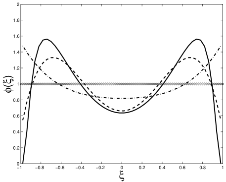
Figure 1: Different type of twist-3 DA. The solid line is for our $\phi_{p}(\xi)$. And for comparison, we list the asymptotic DA, the DAs of Ref.huang3 and Refs.Braun2 ; ball2 in diamond line, the dashed line and the dash-dot line respectively.

In Fig.(1), we show our $\phi_{p}(\xi)$ in solid line, and for comparison, we also present the asymptotic DA, the DAs of Ref.huang3 and Refs.Braun2 ; ball2 in the diamond line, the dashed line and the dash-dot line, respectively. One may observe that the possible end-point singularity coming from the hard scattering kernel will be suppressed in our DA and the twist-3 contribution can be greatly suppressed at the present experimentally accessible energy region.

III the twist-3 contribution to the pion form factor in the modified pQCD approach

In the large $Q^{2}$ region, by considering only the lowest valence quark state of the pion (i.e. $n=m=2$ in Eq.(2)) and by doing the Fourier transformation of the wave function with the formula,

$$\psi(x_{i},{\bf k}_{\perp};\mu_{f})=\int\frac{d^{2}{\bf b}}{(2\pi)^{2}}e^{-i{\bf b}\cdot{\bf k_{\perp}}}\hat{\psi}(x_{i},{\bf b};\mu_{f}),$$

we can transform the pion form factor Eq.(2) into the compact parameter $\mathbf{b}$ spacelis ; nli ,

$$F_{\pi}(Q^{2}) = \int[dx_{i}d{\bf b}][dy_{j}d{\bf h}]\hat{\psi}(x_{i},{\bf b};\mu_{f})\hat{T}(x_{i},{\bf b};y_{j},{\bf h};\mu_{f})\hat{\psi}(y_{j},{\bf h};\mu_{f})\times S_{t}(x_{i})S_{t}(y_{j})\times$$ (13)

$$\exp(-S(x_{i},y_{j},Q,\mathbf{b},\mathbf{h};\mu_{f})),$$

where $\hat{\mu}_{f}=\ln(\mu_{f}/\Lambda_{QCD})$, $[dx_{i}d{\bf b}]=dx_{1}dx_{2}d^{2}\mathbf{b}\delta(1-x_{1}-x_{2})/(16\pi^{3})$ and the hard kernel

$$\hat{T}(x_{i},{\bf b};y_{j},{\bf h};\mu_{f})=\int\frac{d^{2}{\bf k}_{\perp}}{(2\pi)^{2}}\frac{d^{2}{\bf l}_{\perp}}{(2\pi)^{2}}e^{-i{\bf b}\cdot{\bf k_{\perp}}-i{\bf h}\cdot{\bf l_{\perp}}}T(x_{i},{\bf k}_{\perp i};y_{j},{\bf l}_{\perp j};\mu_{f}).$$

The factor $\exp(-S(x_{i},y_{j},Q,\mathbf{b},\mathbf{h};\mu_{f}))$ contains the Sudakov logarithmic corrections and the renormalization group evolution effects of both the wave functions and the hard scattering amplitude,

$$S(x_{1},y_{1},Q,\mathbf{b},\mathbf{h};\mu_{f})=\left[\left(\sum_{i=1}^{2}s(x_{i},b,Q)+\sum_{j=1}^{2}s(y_{j},h,Q)\right)-\frac{1}{\beta_{1}}\ln\frac{\hat{\mu}_{f}}{\hat{b}}-\frac{1}{\beta_{1}}\ln\frac{\hat{\mu}_{f}}{\hat{h}}\right],$$ (14)

where ${\hat{b}}\equiv{\rm ln}(1/b\Lambda_{QCD})$, ${\hat{h}}\equiv{\rm ln}(1/h\Lambda_{QCD})$ and $s(x,b,Q)$ is the Sudakov exponent factor, whose explicit form up to next-to-leading log approximation can be found in Ref.liyu . In Eq.(13), $S_{t}(x_{i})$ and $S_{t}(y_{i})$ come from the threshold resummation effects and the exact form of each involves one parameter integrationkls . In order to simplify the numerical calculations, we take a simple parametrization proposed in Ref.kls ,

$$S_{t}(x)=\frac{2^{1+2c}\Gamma(3/2+c)}{\sqrt{\pi}\Gamma(1+c)}[x(1-x)]^{c}\;,$$ (15)

where the parameter $c$ is determined around $0.3$ for the pion case.

To obtain the momentum projector for the pion, one may take the Fourier transformation of the bilocal operator matrix element defined in Eq.(3)BenekeFeldmann ,

$$M_{\alpha\beta}^{\pi}=\frac{if_{\pi}}{4}\Bigg{\{}/\!\!\!p\,\gamma_{5}\,\psi_{\pi}(x,\mathbf{k_{\perp}})-m^{p}_{0}\gamma_{5}\left(\psi_{p}(x,\mathbf{k_{\perp}})-i\sigma_{\mu\nu}\left(n^{\mu}\bar{n}^{\nu}\,\frac{\psi_{\sigma}^{\prime}(x,\mathbf{k_{\perp}})}{6}-p^{\mu}\,\frac{\psi_{\sigma}(x,\mathbf{k_{\perp}})}{6}\,\frac{\partial}{\partial\mathbf{k}_{\perp\nu}}\right)\right)\Bigg{\}}_{\alpha\beta},$$ (16)

where $\psi_{\sigma}^{\prime}(x,\mathbf{k_{\perp}})=\partial\psi_{\sigma}(x,\mathbf{k_{\perp}})/\partial x$. $n=(1,0,\mathbf{0}_{\bot})$ and $\bar{n}=(0,1,\mathbf{0}_{\bot})$ are two unit vectors that point to the plus and the minus directions, respectively. Note we have used the parameter $m^{p}_{0}$ to replace the factor $\mu_{\pi}$ in Eq.(16).

With the help of the above equations, the final formula for the pion form factor in the modified pQCD approach can be written as,

$$F_{\pi}(Q^{2}) = \frac{16}{9}\pi f^{2}_{\pi}Q^{2}\int_{0}^{1}dxdy\int_{0}^{\infty}bdbhdh\alpha_{s}(\mu_{f})\times\left[\frac{\bar{y}}{2}\hat{\psi}_{\pi}(x,b;\mu_{f})\hat{\psi}^{*}_{\pi}(y,h;\mu_{f})+\right.$$ (17)

$$\frac{(m^{p}_{0})^{2}}{Q^{2}}\left(y\hat{\psi}_{p}(x,b;\mu_{f})\hat{\psi}^{*}_{p}(y,h;\mu_{f})+(1+\bar{y})\hat{\psi}_{p}(x,b;\mu_{f})\frac{\hat{\psi}^{\prime*}_{\sigma}(y,h;\mu_{f})}{6}+\right.$$

$$\left.\left.3\hat{\psi}_{p}(x,b;\mu_{f})\frac{\hat{\psi}^{*}_{\sigma}(y,h;\mu_{f})}{6}\right)\right]\hat{T}(x,{\bf b};y,{\bf h};\mu_{f})\times S_{t}(x_{i})S_{t}(y_{j})\times$$

$$\exp(-S(x_{i},y_{j},Q,\mathbf{b},\mathbf{h};\mu_{f}))\ ,$$

where $\bar{x}=(1-x)$, $\bar{y}=(1-y)$ and $\hat{\psi}^{\prime*}_{\sigma}(y,h;\mu_{f})=\partial\hat{\psi}^{*}_{\sigma}(y,h;\mu_{f})/\partial y$. The first term in the square bracket gives the general twist-2 contribution and the remaining terms that are proportional to an overall factor $((m^{p}_{0})^{2}/Q^{2})$ give the twist-3 contribution. The hard scattering amplitude $\hat{T}(x,{\bf b};y,{\bf h};\mu_{f})$ is given by

$$\hat{T}(x,{\bf b};y,{\bf h};\mu_{f}) = K_{0}\left(\sqrt{\bar{x}\bar{y}}Qb\right)\Big{(}\theta(b-h)K_{0}\left(\sqrt{\bar{y}}Qb\right)I_{0}\left(\sqrt{\bar{y}}Qh\right)+$$ (18)

$$\theta(h-b)K_{0}\left(\sqrt{\bar{y}}Qh\right)I_{0}\left(\sqrt{\bar{y}}Qb\right)\Big{)},$$

where the higher power suppressed terms such as $(\mathbf{k_{\perp}}^{2}/Q^{2})$ has been neglected in the numerator, $I_{0}$ and $K_{0}$ are the modified Bessel functions of the first kind and the second kind respectively. If taking out the threshold factors and absorbing the Sudakov factor into the definition of the wave functions, Eq.(17) agrees with Eq.(8) in Ref.weiy (the factor before $\left(\hat{\psi}_{p}(x,b;\mu_{f})\hat{\psi}^{*}_{\sigma}(y,h;\mu_{f})/6\right)$ should be 3 other than 2 obtained there.). To ensure that the pQCD approach is really applicable, one has to specify carefully the renormalization scale $\mu_{f}$ in the strong coupling constant. There are many equivalent ways to do so, a popular way is to freeze $\alpha_{s}(Q^{2})$ at lower $Q^{2}$huangt ; mack ; parisi ; curci ; bjp . Here we take the scheme that is proposed in Refs.lis ; weiy , i.e. its value is taken as the largest renormalization scale associated with the exchanged virtual gluon in the longitudinal and transverse degrees,

$$\mu_{f}=\max(\sqrt{\bar{x}\bar{y}}Q,1/b,1/h),$$ (19)

The Landau pole in the coupling constant at $\mu_{f}=\Lambda_{QCD}$ can be safely avoided in this way.

Table 1: The full form of the LC wave function $\psi^{f}(x,\mathbf{k_{\perp}})=\psi(x,\mathbf{k_{\perp}})\chi_{\pi}$ with the helicity function $\chi_{\pi}$ being included. $\psi^{f}(x,\mathbf{k_{\perp}})$ stands for $\psi^{f}_{\pi}(x,\mathbf{k_{\perp}})$, $\psi^{f}_{p}(x,\mathbf{k_{\perp}})$ and $\psi^{f}_{\sigma}(x,\mathbf{k_{\perp}})$, respectively.

$\lambda_{1}\lambda_{2}$	$\uparrow\uparrow$	$\uparrow\downarrow$	$\downarrow\uparrow$	$\downarrow\downarrow$
$\psi^{f}_{\lambda_{1}\lambda_{2}}(x,\mathbf{k_{\perp}})$	$-\frac{k_{x}-ik_{y}}{\sqrt{2(m^{2}+k^{2})}}\psi(x,\mathbf{k_{\perp}})$	$\frac{m}{\sqrt{2(m^{2}+k^{2})}}\psi(x,\mathbf{k_{\perp}})$	$-\frac{m}{\sqrt{2(m^{2}+k^{2})}}\psi(x,\mathbf{k_{\perp}})$	$-\frac{k_{x}+ik_{y}}{\sqrt{2(m^{2}+k^{2})}}\psi(x,\mathbf{k_{\perp}})$

Only the usual helicity components $(\lambda_{1}+\lambda_{2}=0)$ in the pion wave function have been considered in Eq.(17). From Eq.(31) in the appendix, one may observe that the full form of the pion LC wave function have four helicity components (Table. 1): namely,

$$\psi^{f}=(\psi^{f}_{\uparrow\uparrow},\psi^{f}_{\uparrow\downarrow},\psi^{f}_{\downarrow\uparrow},\psi^{f}_{\downarrow\downarrow}),\;\;\;\;(\psi^{f}=\psi^{f}_{\pi},\;\psi^{f}_{p},\;\psi^{f}_{\sigma})$$ (20)

By including the higher helicity components into the pion form factor, Eq.(17) can be improved as

$$F_{\pi}(Q^{2}) = \frac{16}{9}\pi f^{2}_{\pi}Q^{2}\int_{0}^{1}dxdy\int_{0}^{\infty}bdbhdh\alpha_{s}(\mu_{f})\times\left[\frac{\bar{y}}{2}\sum_{\lambda_{1}\lambda_{2}}{\cal P}(\hat{\psi}^{f}_{\pi},\lambda_{1},\lambda_{2})+\right.$$ (21)

$$\frac{(m^{p}_{0})^{2}}{Q^{2}}\left(y\sum_{\lambda_{1}\lambda_{2}}{\cal P}(\hat{\psi}^{f}_{p},\lambda_{1},\lambda_{2})+\frac{(1+\bar{y})}{6}\sum_{\lambda_{1}\lambda_{2}}{\cal P}(\hat{\psi}^{f^{\prime}}_{\sigma},\lambda_{1},\lambda_{2})+\right.$$

$$\left.\left.\frac{1}{2}\sum_{\lambda_{1}\lambda_{2}}{\cal P}(\hat{\psi}^{f}_{\sigma},\lambda_{1},\lambda_{2})\right)\right]\hat{T}(x,{\bf b};y,{\bf h};\mu_{f})\times S_{t}(x_{i})S_{t}(y_{j})\times$$

$$\exp(-S(x_{i},y_{j},Q,\mathbf{b},\mathbf{h};\mu_{f}))\ ,$$

where $\hat{\psi}^{f^{\prime}}_{\sigma}=\partial\hat{\psi}^{f}_{\sigma}/\partial x$ and

$$\sum_{\lambda_{1}\lambda_{2}}{\cal P}(\hat{\psi}^{f}_{\pi},\lambda_{1},\lambda_{2})=(\hat{\psi}^{f*}_{\pi\uparrow\downarrow}\hat{\psi}^{f}_{\pi\uparrow\downarrow}+\hat{\psi}^{f*}_{\pi\downarrow\uparrow}\hat{\psi}^{f}_{\pi\downarrow\uparrow})-(\hat{\psi}^{f*}_{\pi\uparrow\uparrow}\hat{\psi}^{f}_{\pi\uparrow\uparrow}+\hat{\psi}^{f*}_{\pi\downarrow\downarrow}\hat{\psi}^{f}_{\pi\downarrow\downarrow}),$$

$$\sum_{\lambda_{1}\lambda_{2}}{\cal P}(\hat{\psi}^{f}_{p},\lambda_{1},\lambda_{2})=(\hat{\psi}^{f*}_{p\uparrow\downarrow}\hat{\psi}^{f}_{p\uparrow\downarrow}+\hat{\psi}^{f*}_{p\downarrow\uparrow}\hat{\psi}^{f}_{p\downarrow\uparrow})-(\hat{\psi}^{f*}_{p\uparrow\uparrow}\hat{\psi}^{f}_{p\uparrow\uparrow}+\hat{\psi}^{f*}_{p\downarrow\downarrow}\hat{\psi}^{f}_{p\downarrow\downarrow}),$$

$$\sum_{\lambda_{1}\lambda_{2}}{\cal P}(\hat{\psi}^{f^{\prime}}_{\sigma},\lambda_{1},\lambda_{2})=(\hat{\psi}^{f*}_{p\uparrow\downarrow}\hat{\psi}^{f^{\prime}}_{\sigma\uparrow\downarrow}+\hat{\psi}^{f*}_{p\downarrow\uparrow}\hat{\psi}^{f^{\prime}}_{\sigma\downarrow\uparrow})-(\hat{\psi}^{f*}_{p\uparrow\uparrow}\hat{\psi}^{f^{\prime}}_{\sigma\uparrow\uparrow}+\hat{\psi}^{f*}_{p\downarrow\downarrow}\hat{\psi}^{f^{\prime}}_{\sigma\downarrow\downarrow}),$$

$$\sum_{\lambda_{1}\lambda_{2}}{\cal P}(\hat{\psi}^{f}_{\sigma},\lambda_{1},\lambda_{2})=(\hat{\psi}^{f*}_{p\uparrow\downarrow}\hat{\psi}^{f}_{\sigma\uparrow\downarrow}+\hat{\psi}^{f*}_{p\downarrow\uparrow}\hat{\psi}^{f}_{\sigma\downarrow\uparrow})-(\hat{\psi}^{f*}_{p\uparrow\uparrow}\hat{\psi}^{f}_{\sigma\uparrow\uparrow}+\hat{\psi}^{f*}_{p\downarrow\downarrow}\hat{\psi}^{f}_{\sigma\downarrow\downarrow}).$$

In the above equation, because both the photon and the gluon are vector particles, the quark helicity is conserved at each vertex in the limit of vanishing quark masslb . Hence there is no hard-scattering amplitude with the quark’s and the antiquark’s helicities being changed. For the hard scattering amplitude $\hat{T}(x,{\bf b};y,{\bf h};\mu_{f})$, we have implicitly adopted the approximate relation for all the twist structures in Eq.(21), i.e.

$$\hat{T}(x,{\bf b};y,{\bf h};\mu_{f})^{\uparrow\downarrow+\downarrow\uparrow}\approx-\hat{T}(x,{\bf b};y,{\bf h};\mu_{f})^{\uparrow\uparrow+\downarrow\downarrow}.$$ (22)

By ignoring the transverse momentum dependence in the quark propagator and applying the symmetries of the wave functions, especially the fact that $\psi^{f*}_{\uparrow\uparrow}(x,\mathbf{k_{\perp}})=\psi^{f}_{\downarrow\downarrow}(x,\mathbf{k_{\perp}})$, Ref.wk pointed out that the approximate relation Eq.(22) can be strictly satisfied. In fact, when the transverse momentum dependence in the quark propagator has been ignored, the $T_{H}$ depends only on one compact $\mathbf{b}$-space, and Eq.(22) can be changed to a strict one, i.e. $\hat{T}(x,y,{\bf b};\mu_{f})^{\uparrow\downarrow+\downarrow\uparrow}=-\hat{T}(x,y,{\bf b};\mu_{f})^{\uparrow\uparrow+\downarrow\downarrow}$. As is shown in Ref.lis , the transverse momentum dependence in the quark propagator will give about $15\%$ correction at $Q=2GeV$lis , so this effect can not be safely neglected. The hard scattering amplitude for the twist-2 contribution has been strictly calculated in Ref.huangww within the LC pQCD approach. One may find that when all the $k_{T}$ dependence are included, strictly $\hat{T}(x,{\bf b};y,{\bf h};\mu_{f})^{\uparrow\downarrow+\downarrow\uparrow}\neq-\hat{T}(x,{\bf b};y,{\bf h};\mu_{f})^{\uparrow\uparrow+\downarrow\downarrow}$ and Eq.(22) can be approximately satisfied. In the following discussions, we will keep the transverse momentum dependence in the hard scattering amplitude fully and use the approximate relation Eq.(22) to estimate all the helicity components’ contributions to the pion form factor.

Before doing numerical calculations, we would like to mention a few words on the value of $m^{p}_{0}$. Based on the equation of motion of on-shell quarks, the authors used $\mu_{\pi}=m_{\pi}^{2}/(m_{u}+m_{d})\sim 2.0GeV$ instead of $m^{p}_{0}$ for the twist-3 wave functions in Refs.Braun2 ; beneke ; weiy . A running behavior has been introduced in Refs.twist1 ; twist2 ; twist3 ; cdh and with this choice, one may find that the average value for $\mu_{\pi}$ over the intermediate energy region is around $2.5GeV$. In Refs.kls ; ly a smaller phenomenological value $\sim 1.4GeV$, which is consistent with the result obtained from the chiral perturbation theorychiral ; ball2 , is used to fit the B meson to the light meson transition form factors. Based on the moment calculation by applying the QCD sum rules, Ref.huang3 obtained $m^{p}_{0}=1.30\pm 0.06GeV$, which is very close to the above phenomenological value. So to be consistent with our model wave function constructed in the last section, we will take $m^{p}_{0}=1.30GeV$ for our latter discussions.

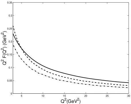
Figure 2: Twist-3 contribution to the pion form factor $Q^{2}F(Q^{2})$, where the second moment of $\psi_{p}(x,\mathbf{k}_{\perp})$ or $\psi^{f}_{p}(x,\mathbf{k}_{\perp})$ is taken to be $\langle\xi^{2}\rangle=0.350$. The dash-dot line and the dashed line are the twist-3 contributions for the full form of the LC wave function with or without considering the $k_{T}$ dependence in the quark propagator. The solid line is for the twist-3 contribution from the LC wave function that contains only the usual helicity component but is normalized to unity.

We show the twist-3 contribution to pion form factor $Q^{2}F(Q^{2})$ with all helicity components (i.e. using the full form of the LC wave functions $\psi^{f}_{p}(x,\mathbf{k_{\perp}})$ and $\psi^{f}_{\sigma}(x,\mathbf{k_{\perp}})$) calculated within the modified pQCD approach in Fig.(2), where the second moment of $\psi^{f}_{p}(x,\mathbf{k}_{\perp})$ is taken to be $\langle\xi^{2}\rangle=0.350$. One may observe that the transverse momentum dependence in the quark propagator will give about $25\%$ correction at $Q^{2}=2GeV$ for the twist-3 contribution, which is bigger than the case of the leading twist contribution. So it is more essential to keep the transverse momentum dependence fully into the hard scattering kernel for the twist-3 contribution. As a comparison, we also show the contribution from the twist-3 wave functions (i.e. $\psi_{p}(x,\mathbf{k_{\perp}})$ and $\psi_{\sigma}(x,\mathbf{k_{\perp}})$) that contain only the usual helicity component but are normalized to unity in Fig.(2). One may find the contribution from the twist-3 wave function that contains only the usual helicity component but is normalized to unity (the solid line) is larger than the contribution from the wave function with all the helicity components being considered (the dash-dot line). It is reasonable and is also the case of the twist-2 contribuionhuangww , because if one normalizes the valence Fock state to unity without including the higher helicity components, then the contribution from the valence state can be enhanced and become important inadequately.

IV Comparison with other models for twist-3 wave function

As has been pointed out in Sec.III, the contribution from the twist-3 wave functions $\psi_{p}(x,\mathbf{k_{\perp}})$ and $\psi_{\sigma}(x,\mathbf{k_{\perp}})$ that contain only the usual helicity components but is normalized to unity is larger than the contribution from the wave functions $\psi^{f}_{p}(x,\mathbf{k_{\perp}})$ and $\psi^{f}_{\sigma}(x,\mathbf{k_{\perp}})$ with all the helicity components being considered. However, as is shown in Fig.(2), since both of the twist-3 contributions have a similar behavior and are close to each other, the qualitative conclusions will be the same. And for easy comparing with the results in the literature, we will take the LC wave functions $\psi_{p}(x,\mathbf{k_{\perp}})$ and $\psi_{\sigma}(x,\mathbf{k_{\perp}})$ that only contain the usual helicity components for the discussions in the present section.

Because of the end-point singularity, the twist-3 contribution depends heavily on the twist-3 wave function, especially on $\psi_{p}(x,\mathbf{k_{\perp}})$. In this section, we will do a comparative study on the twist-3 contribution from different type of $\psi_{p}(x,\mathbf{k_{\perp}})$. For this purpose, we take Eq.(17) to calculate the pion form factor, in which only the usual helicity components in the wave functions have been taken into consideration.

The twist-2 and twist-3 wave functions $\psi_{\pi}$, $\psi_{p}$ and $\psi_{\sigma}$ may have different transverse momentum dependence, and for simplicity, we assume the same transverse momentum dependence for these space wave functions. For the transverse momentum dependence of the wave function, we take a simple Gaussian form, i.e.

$$\Sigma(x,\mathbf{k_{\perp}})=\frac{A}{g(x)}\exp\left(-\frac{m^{2}+k_{\perp}^{2}}{8\beta^{2}g(x)}\right),$$ (23)

where $A$ is the normalization factor, $g(x)$ is either $1$ or $x(1-x)$. When $g(x)=x(1-x)$, it is agree with the BHL prescription mentioned in Sec.II. After making the Fourier transformation, Eq.(23) can be transformed into the compact parameter $\mathbf{b}$ space as,

$$\Sigma(x,\mathbf{b})=\frac{2\pi A}{g(x)}\int_{0}^{1/b}\exp\left(-\frac{m^{2}+k^{2}_{\perp}}{8\beta^{2}g(x)}\right)J_{0}(bk_{\perp})k_{\perp}dk_{\perp}\ ,$$ (24)

where the upper limit $(1/b)$ is necessary to insure the wave function to be “soft”botts ; ch1 .

Next, we consider the pion wave functions. The twist-2 wave function $\psi_{\pi}(x,\mathbf{k_{\perp}})$ with the prescription Eq.(6) can be written as

$$\psi_{\pi}(x,\mathbf{k_{\perp}})=A_{\pi}\exp\left(-\frac{m^{2}+k_{\perp}^{2}}{8\beta^{2}x(1-x)}\right),$$ (25)

where the parameters can be determined by the normalization condition of the wave functionBenekeFeldmann

$$\int^{1}_{0}dx\int\frac{d^{2}{\bf k}_{\perp}}{16\pi^{3}}\psi_{\pi}(x,{\bf k}_{\perp})=1\ ,$$ (26)

and some necessary constraintshms . Taking the parameter values in Eq.(9), we obtain $A_{\pi}=1.187\times 10^{-3}MeV^{-2}$. The asymptotic form of twist-3 DA $\phi_{\sigma}(x)$ is the same as that of $\phi_{\pi}(x)$, and the end-point singularity coming from the hard scattering amplitude can also be cured. So for $\phi_{\sigma}(x)$ we also take its asymptotic form. For the twist-3 contribution to the pion form factor, the main difference for the existed resultsweiy ; cdh ; twist1 ; twist2 ; twist3 comes mainly from the different models for $\psi_{p}(x,\mathbf{k_{\perp}})$. The difference caused by the different model of $\psi_{\sigma}(x,\mathbf{k_{\perp}})$ (if all of them are asymptotic like) are quite small, so in the following, we will only consider the difference caused by different type of $\psi_{p}(x,\mathbf{k_{\perp}})$ and the contribution from $\psi_{\sigma}(x,\mathbf{k_{\perp}})$ will be included as a default with the fixed asymptotic form for its DA and the same $k_{T}$ dependence as $\psi_{p}(x,\mathbf{k_{\perp}})$.

In the asymptotic limit, $\phi^{as}_{p}(x)=1$, the end-point singularity coming from the hard scattering amplitude can not be cured, and the model dependence of $\phi_{p}(x)$ is much more involved. Taking the asymptotic DA and ignoring the $k_{T}$ dependence in the wave function, Refs.cdh ; twist1 ; twist2 obtained a much larger contribution in a wide energy region $2GeV^{2}<Q^{2}<40GeV^{2}$, comparing with the twist-2 contribution. Using the model wave function of $\psi_{p}(x,\mathbf{k_{\perp}})$ constructed in Sec.II, one may find that the twist-3 contributions are suppressed certainly.

Table 2: The first three moments for the twist-2 and the twist-3 wave functions, where all the full form of LC wave functions have the same BHL-like $k_{T}$ dependence, $\psi^{f}_{\pi}$($\psi^{f}_{\sigma})=\psi_{\pi}$($\psi_{\sigma})\chi_{\pi}$ and $\psi^{f}_{p}=\psi_{p}\chi_{\pi}$.

-	without Wigner rotation					with Wigner rotation
-	$\psi_{\pi}$/$\psi_{\sigma}$	$\psi_{p}$	$\psi^{(1)}_{p}$	$\psi^{(2)}_{p}$	$\psi^{(3)}_{p}$	$\psi^{f}_{\pi}$/$\psi^{f}_{\sigma}$	$\psi^{f}_{p}$
$\langle\xi^{0}\rangle$	1	1	1	1	1	1	1
$\langle\xi^{2}\rangle$	0.167	0.350	0.333	0.391	0.352	0.176	0.350
$\langle\xi^{4}\rangle$	0.060	0.185	0.200	0.251	0.197	0.066	0.185

To study this effects more clearly, we compare our model with three different types of $\psi_{p}(x,\mathbf{k_{\perp}})$. In the literature, most of the calculations on the twist-3 contribution of the pion take $\phi_{p}(x)$ as $\psi_{p}(x,\mathbf{k_{\perp}})$, i.e. without considering the intrinsic $k_{T}$ dependence in the wave function, some examples for the electromagnetic pion form factor can be found in Refs.cdh ; twist1 ; twist2 and examples for the $B\to\pi$ form factor can be found in Refs.ly ; kls . However, as has been argued in several papershuangww ; weiy ; jk , the intrinsic transverse momentum dependence in the wave function is very important for the pion form factor and the results will be overestimated without including this effect. So in our comparison, the three different type of wave functions are constructed by adding a common simple Gaussian form (Eq.(23) with $g(x)=1$) to three different type of distribution amplitudes used in the literature, i.e. the one of asymptotic behavior, the one in Ref.Braun2 and the one in Ref.huang3 respectively,

$$\psi^{(1)}_{p}(x,\mathbf{k_{\perp}}) = A^{\prime}_{p}\exp\left(-\frac{k_{\perp}^{2}}{8\beta^{{}^{\prime}2}}\right),$$ (27)

$$\psi^{(2)}_{p}(x,\mathbf{k_{\perp}}) = (1+0.43C_{2}^{1/2}(2x-1)+0.09C_{4}^{1/2}(2x-1))A^{\prime}_{p}\exp\left(-\frac{k_{\perp}^{2}}{8\beta^{{}^{\prime}2}}\right),$$ (28)

$$\psi^{(3)}_{p}(x,\mathbf{k}_{\perp}) = (1+0.137C_{2}^{1/2}(2x-1)-0.721C_{4}^{1/2}(2x-1))A^{\prime}_{p}\exp\left(-\frac{k^{2}_{\perp}}{8\beta^{{}^{\prime}2}}\right).$$ (29)

The parameters $A^{\prime}_{p}$ and $\beta^{\prime}$ can be determined from the similar wave function normalization condition as Eq.(26), $A^{\prime}_{p}=7.025\times 10^{-4}MeV^{-2}$ and $\beta^{\prime}=168MeV$. For the wave functions $\psi^{(i)}_{p}$ ($i=1,2,3$), the harmonic parameter $\beta^{\prime}$ is different from that of $\psi_{\pi}(x,\mathbf{k_{\perp}})$, however it can be taken as an effective/average value of the harmonic parameter with $m=0$ and $g(x)=1$. The moments of the corresponding DAs are listed in Table.2.

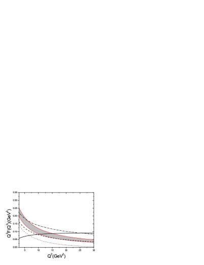
(a)

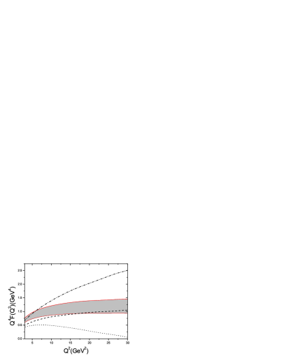
(b)

Figure 3: Different twist-3 wave function’s contribution to the pion form factor, where the left diagram is for $Q^{2}F(Q^{2})$ and the right is for $Q^{4}F(Q^{2})$. The dashed line, the dash-dot line and the dotted line are for $\psi^{(1)}_{p}(x,\mathbf{k_{\perp}})$, $\psi^{(2)}_{p}(x,\mathbf{k_{\perp}})$ and $\psi^{(3)}_{p}(x,\mathbf{k_{\perp}})$ respectively. The contribution from our model wave function $\psi_{p}(x,\mathbf{k_{\perp}})$ with varying second moment $\langle\xi^{2}\rangle$ is shown by a shaded band, whose lower and upper edges correspond to $\langle\xi^{2}\rangle=0.320,0.370$ respectively. For comparison, the twist-2 contribution from $\psi_{\pi}(x,\mathbf{k_{\perp}})$ is shown in solid line.

We show the contributions to the pion form factor from the different model for $\psi_{p}(x,\mathbf{k_{\perp}})$ in Figs.(3a,3b), where the contribution from our model wave function $\psi_{p}(x,\mathbf{k_{\perp}})$ with varying second moment $\langle\xi^{2}\rangle$ is shown by a shaded band and the twist-2 contribution from $\psi_{\pi}(x,\mathbf{k_{\perp}})$ is included in Fig.(3a) for comparison. Our present result for $\psi^{(1)}_{p}(x,\mathbf{k_{\perp}})$ (in dashed line) is much lower than the result shown in Ref.weiy , since the value of $\mu_{\pi}$ used there has been changed to the present value of $m^{p}_{0}$. One may observe that the twist-3 contribution is improved with our model wave function, and for the case of $\langle\xi^{2}\rangle=0.350$, at about $Q^{2}=30GeV^{2}$, it is only about $45\%$ comparing with the twist-2 contribution. This behavior is quite different from the previous observationsweiy ; cdh ; twist1 ; twist2 ; twist3 , where they concluded that the twist-3 contribution to the pion form factor is comparable or even larger than that of the leading twist in a wide intermediate energy region.

As is shown in Figs.(3a,3b), the twist-3 contribution from $\psi^{(1)}_{p}(x,\mathbf{k_{\perp}})$ is comparable to our model wave function, which also has the right power behavior. We take a simple Gaussian behavior (Eq.(23) with $g(x)=1$) for the transverse momentum dependence in $\psi^{(1)}_{p}(x,\mathbf{k_{\perp}})$, i.e. a complete factorization between longitudinal and transverse momentum-dependence in the wave function. This Gaussian distribution behavior shows a strong dumping at large transverse distances, $\sim\exp(-2\beta^{2}b^{2})$, while our model function with the prescription Eq.(6) has a slow-dumping with oscillatory behavior, $\sim\cos\left(\sqrt{x(1-x)}b\beta^{2}-\pi/4\right)/\sqrt{b}$. If we also take the simple transverse momentum behavior in our model wave function, i.e. the one as $\psi_{p}^{(3)}(x,\mathbf{k_{\perp}})$, we find that the twist-3 contribution will be even lower, which is shown clearly by the dotted line in Figs.(3a,3b). However as is shown in Fig.(3b), we can not achieve a right power behavior with $\psi_{p}^{(3)}(x,\mathbf{k_{\perp}})$, i.e. it drops down too quickly.

Finally, with our model wave function for $\psi_{p}(x,\mathbf{k})$, we discuss the model dependence of the twist-3 contribution on the DA moments $\langle\xi^{2n}\rangle$. Here we take the second moment $\langle\xi^{2}\rangle$, which gives the main contribution to $\phi_{p}(\xi)$, as an example. Varying the second moment $\langle\xi^{2}\rangle$ within a broader range, i.e. $\langle\xi^{2}\rangle\in(0.320,0.370)$, and adjusting the fourth moment $\langle\xi^{4}\rangle$ to make $\phi_{p}(\xi)$ has a closed behavior as the one that is obtained in Ref.huang3 (i.e. the dashed line in Fig.(1)), we can determine the corresponding parameters $A_{p}$, $B_{p}$ and $C_{p}$ in the wave function $\psi_{p}(x,\mathbf{k})$. The twist-3 contribution to the pion form factor with varying second moment $\langle\xi^{2}\rangle$ has been shown by a shaded band in Figs.(3a,3b). One may observe that the pionic twist-3 contribution increases with the increment of $\langle\xi^{2}\rangle$ and all has a quite similar behavior on the variation of the energy scale $Q^{2}$, i.e. as is shown in Fig.(3b), the right asymptotic power behavior of order $1/Q^{4}$ has already been achieved at the present experimentally accessible energy region.

V summary and discussion

In this paper, we have constructed a model wave function for $\psi_{p}(x,\mathbf{k_{\perp}})$ based on the moment calculationhuang3 by using the QCD sum rule approach. It has a better end-point behavior than that of the asymptotic one and its moments are consistent with the QCD sum rule results. Although its moments are slightly different from that of the asymptotic DA, its better end-point behavior will cure the end-point singularity of the hard scattering amplitude and its contribution will not be overestimated at all.

With this model wave function, by keeping the $k_{T}$ dependence in the wave function and taking the Sudakov effects and the threshold effects into account, we have carefully studied the twist-3 contributions to the pion form factor. Comparing the different models for $\psi_{p}(x,\mathbf{k_{\perp}})$, a detailed study on the twist-3 contribution to the pion form factor has been given within the modified pQCD approach. It has been shown that our model wave function $\psi_{p}(x,\mathbf{k_{\perp}})$ can give the right power behavior for the twist-3 contribution. With the present model wave function defined in Eq.(8) for $\psi_{p}(x,\mathbf{k_{\perp}})$, our results predict that, at about $Q^{2}\sim 10GeV^{2}$, the twist-3 contribution begins to be less than the twist-2 contribution, and for the wave function $\psi_{p}(x,\mathbf{k}_{\perp})$ with $\langle\xi^{2}\rangle=0.350$ at about $Q^{2}=30GeV^{2}$, it is only about $45\%$ comparing with the twist-2 contribution. This behavior is quite different from the previous observationsweiy ; cdh ; twist1 ; twist2 ; twist3 , where they concluded that the twist-3 contribution to the pion form factor is comparable or even larger than that of the leading twist in a wide intermediate energy region up to $40GeV^{2}$. The higher helicity components $(\lambda_{1}+\lambda_{2}=\pm 1)$ in the twist-3 wave function that come from the spin-space Wigner rotation have also been considered. The higher helicity components in the twist-3 wave function will do a further suppression to the contribution from the usual helicity components $(\lambda_{1}+\lambda_{2}=0)$, and at about $Q^{2}=5GeV^{2}$, it will give $\sim 10\%$ suppression.

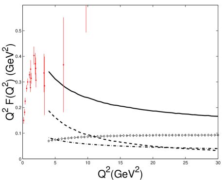
Figure 4: Perturbative prediction for the pion form factor. The diamond line, the dash-dot line, the dashed line and the solid line are for LO twist-2 contribution, the approximate NLO twist-2 contributionfield ; melic , the twist-3 contribution and the combined total hard contribution, respectively. The experimental data are taken fromcjb .

In Fig.(4), we show the combined hard contributions for the twist-2 and twist-3 contributions to the pion form factor, where the higher helicity components have been included in both the twist-2 and the twit-3 wave functions, and the twist-3 contribution has been calculated with our model wave function $\psi^{f}_{p}(x,\mathbf{k_{\perp}})$ with $\langle\xi^{2}\rangle=0.350$. As has been pointed out in Refs.huangt ; lis , the applicability of pQCD to the pion form factor can only be achieved at a momentum transfer bigger than $Q^{2}\sim 4GeV^{2}$, so in Fig.(4), all the curves are started at $Q^{2}=4GeV^{2}$. Together with the NLO corrections to the twist-2 contributions, which for the asymptotic DA, with the renormalization scale $\mu_{R}$ and the factorization scale $\mu_{f}$ taken to be $\mu^{2}_{R}=\mu^{2}_{f}=Q^{2}$, can roughly be taken asfield ; melic , $Q^{2}F^{NLO}_{\pi}\approx(0.903GeV^{2})\alpha^{2}_{s}(Q^{2})$, one may find that the combined total hard contribution do not exceed and will reach the present experimental data. There is still a room for the other power corrections, such as the higher Fock states’ contributionsbakker ; melo , soft contributions etc.. Finally, we will conclude that there is no any problem with applying the pQCD theory including all power corrections to the exclusive processes at $Q^{2}>$ a few $GeV^{2}$.

Acknowledgements

This work was supported in part by the Natural Science Foundation of China (NSFC). And the authors would like to thank M.Z. Zhou and X.H. Wu for some useful discussions.

Appendix A full form for the LC wave function

By doing the spin-space Wigner rotation, we can transform the ordinary equal-time (instant-form) spin-space wave function in the rest frame into that in the LC dynamics. After doing the Wigner rotation, the covariant form for the pion helicity functions can be written ashms ; jaus ,

$$\chi_{\pi}(x,\mathbf{k_{\perp}})=\frac{1}{\sqrt{2}\tilde{M}_{0}}\bar{u}(p_{1},\lambda_{1})\gamma_{5}v(p_{2},\lambda_{2}),$$ (30)

where $p_{1}=(x,\mathbf{k_{\perp}})$ and $p_{2}=(\bar{x},-\mathbf{k_{\perp}})$ ($\bar{x}=1-x$) are the momenta of the two constituent quarks in the pion, $\tilde{M}_{0}^{2}=(m^{2}+k^{2})/x(1-x)$ and the LC spinors $u$ and $v$ have the Wigner rotation built into them. Then the full form of the LC wave function can be written as

$$\psi^{f}(x,\mathbf{k_{\perp}})=\psi(x,\mathbf{k_{\perp}})\chi_{\pi}(x,\mathbf{k_{\perp}}),$$ (31)

where the momentum space wave function $\psi(x,\mathbf{k_{\perp}})$ represents $\psi_{p}(x,\mathbf{k_{\perp}})$, $\psi_{\pi}(x,\mathbf{k_{\perp}})$ and $\psi_{\sigma}(x,\mathbf{k_{\perp}})$ respectively. Because all the LC wave functions can be dealt with in a similar way, here we only take $\psi_{p}(x,\mathbf{k_{\perp}})$ that is defined in Eq.(8) as an explicit example to show how to determine the parameters in the full form.

The full form of LC wave function $\psi^{f}_{p}(x,\mathbf{k_{\perp}})$ contains all the helicity components’ contributions and its four components can be found in Table.1. The parameter values built in the wave function $\psi^{f}_{p}(x,\mathbf{k_{\perp}})$ can be done in a similar way as for the wave function of $\psi_{p}(x,\mathbf{k_{\perp}})$ that contains only the usual helicity components, i.e.

$$A_{p}=4.088\times 10^{-4}MeV^{-2},\;\;B_{p}=1.077,\;\;C_{p}=-4.317\times 10^{-3}$$ (32)

$$m=309.6MeV,\;\;\;\beta=395.9MeV,\;\;\;{\rm for}\;\;\;\langle\mathbf{k_{\perp}}^{2}\rangle\approx(367MeV)^{2}$$ (33)

where the parameters $m$, $\beta$ are determined by the wave function normalization condition and some necessary constraintshms , and the values of $A_{p}$, $B_{p}$ and $C_{p}$ are determined by requiring the first three moments of its DA to be the values shown in Eq.(11). From the wave function Eq.(31), we obtain

$$\phi^{f}_{p}(\xi)=\frac{A_{p}m\beta}{\pi^{3/2}\sqrt{2(1-\xi^{2})}}(1+B_{p}C^{1/2}_{2}(\xi)+C_{p}C^{1/2}_{4}(\xi))\exp\left(1-Erf\left(\sqrt{\frac{m^{2}}{2\beta^{2}(1-\xi^{2})}}\right)\right),$$ (34)

where the error function $Erf(x)$ is defined as $Erf(x)=\frac{2}{\sqrt{\pi}}\int_{0}^{x}e^{-t^{2}}dt$. One may find that $\phi^{f}_{p}(\xi)$ is almost coincide with $\phi_{p}(\xi)$ that is shown in Eq.(10), and for simplicity, we can take the approximate relation, $\phi^{f}_{p}(\xi)\approx\phi_{p}(\xi)$. It is reasonable because we have adjusted the parameters in both DAs to have the same moments and due the fact that the momentum space wave function $\psi_{p}(x,\mathbf{k_{\perp}})$ is an even function of $\mathbf{k_{\perp}}$, one may find that the higher helicity components in $\psi^{f}_{p}(x,\mathbf{k_{\perp}})$ do not contribute to $\phi^{f}_{p}(\xi)$.

References

- (1) N. Isgur and C.H. Llewellyn Smith, Phys.Rev. Lett 52, 1080(1984); Phys. Lett. B217, 535(1989); Nucl.Phys. B317, 526(1989).
- (2) H.N. Li and G. Sterman, Nucl.Phys. B381, 129(1992).
- (3) C.R. Ji, A. Pang and A. Szczepaniak, Phys.Rev. D52, 4038(1995).
- (4) F.G. Cao, J. Cao, T. Huang and B.Q. Ma, Phys.Rev. D55, 7107(1997).
- (5) A. Szczepaniak, C.R. Ji and A. Radyushkin, Phys. Rev. D 57, 2813 (1998).
- (6) M. Beneke and Th. Feldmann, Nucl.Phys. B592, 3(2001); Z.T. Wei and M.Z. Yang, Nucl.Phys. B642, 263(2002).
- (7) S. Eidelman etal., Phys. Lett. B592, 1(2004).
- (8) V.M. Braun and I.E. Filyanov, Z.Phys. C48, 239(1990).
- (9) T. Huang and Q.X. Shen, Z.Phys. C50, 139(1991).
- (10) R.D. Field, R. Gupta, S. Otto and L. Chang, Nucl.Phys. B186, 429(1981).
- (11) G. Grunberg, hep-ph/9705290; in Proceedings of the 32nd Rencontres de Moriond: QCD and High-Energy Hadronic Interactions, Les Arces, France, 22-29, March 1997, edited by J.Tran Thanh Van (Editions Frontieres, 1997) p.673 (hep-ph/9705460).
- (12) B.R. Webber, Nucl.Phys.Proc. Suppl.71, 66(1999); M. Dasgupta and B.R. Webber, Phys.Lett. B382, 273(1996).
- (13) N.G. Stefanis, W. Schroers and H.-Ch. Kim, Eur.Phys.J. C18, 137(2000).
- (14) R. Akhoury, V.I. Zakharov, in 5th International Conference on Physics Beyond the Standard Model, Balholm, Norway, 29 April-4 May 1997, p.274(hep-ph/9705318); Nucl.Phys.Proc. Suppl.64, 350(1998); Phys.Lett. B438, 165(1998).
- (15) N.V. Krasnikov and A.A. Pivovarov, hep-ph/9510207; hep-ph/9512213; hep-ph/9607247.
- (16) A.P. Bakulev, K. Passek-Kumericki, W. Schroers and N.G. Stefanis, Phys.Rev. D70, 033014(2004); hep-ph/0405062.
- (17) B.Melic, B. Nizic and K. Passek, Phys.Rev. D60, 074004(1999); hep-ph/9908510.
- (18) T. Huang, X.G. Wu and X.H. Wu, Phys.Rev. D70, 053007(2004); hep-ph/0404163.
- (19) A. Szczepaniak, A.G. Williams, Phys.Lett. B302, 87(1993); B.V. Geshkenbein, M.V. Terentyev, Phys.Lett. B117, 243(1982).
- (20) C.S. Huang, Commun.Theor.Phys. 2, 1265(1983).
- (21) V.L. Chernyak, A.R. Zhitnitsky, Phys. Rep. 112, 173(1984); B.V. Geshkenbein, M.V. Terentev, Sov.J.Nucl.Phys. 39, 873(1984).
- (22) F.G. Cao, Y.B. Dai and C.S. Huang, Euro.Phys.J. C11, 501(1999).
- (23) Z.T. Wei and M.Z. Yang, Phys.Rev. D67, 094013(2003).
- (24) T. Huang, X.H. Wu and M.Z. Zhou, Phys.Rev. D70, 014013(2004).
- (25) P. Ball, JHEP 9901, 010(1999).
- (26) P. Ball, V.M. Braun, Y. Koike and K. Tanaka, Nucl.Phys. B529, 323(1998).
- (27) S.J. Brodsky, T. Huang and G.P. Lepage, in Particles and Fields, Vol.2, Proceedings of the Banff Summer Institute, Banff, Alberta, 1981, edited by A.Z. Capri and A.N. Kamal (Plenum, New York, 1983), P143; G.P. Lepage, S.J. Brodsky, T.Huang, and P.B. Mackenize, ibid., p83; T. Huang, in Proceedings of XXth International Conference on High Energy Physics, Madison, Wisconsin, 1980, edited by L.Durand and L.G. Pondrom, AIP Conf.Proc.No. 69(AIP, New York, 1981), p1000.
- (28) Z. Dziembowski and L. Mankiewicz, Phys.Rev.Lett. 55, 1839(1985).
- (29) H. Kawamura, J. Kodaira, C.F. Qiao and K. Tanaka, Nucl.Phys.Proc.Suppl. 116, 269(2003).
- (30) P. Ball etal, Nucl.Phys. B529, 323(1998).
- (31) T. Huang, B.Q. Ma and Q.X. Shen, Phys.Rev.D49, 1490(1994).
- (32) S.W. Wang and L.S. Kisslinger, Phys.Rev. D54, 5890(1996).
- (33) M. Nagashima and H.N. Li, Phys. Rev. D67, 034001(2003).
- (34) H.N. Li and H.L. Yu, Phys.Rev. Lett.74, 4388(1995); Phys.Lett. B353, 301(1995); Phys.Rev. D 53, 2480(1996); F.G. Cao, T. Huang and C.W. Luo, Phys.Rev. D52, 5358(1995); H.N. Li, Phys.Rev. D52, 3958(1995).
- (35) T. Kurimoto, H.N. Li and A.I. Sanda, Phys.Rev. D65, 014007(2002); H.N. Li, Phys.Rev.D 66, 094010(2002).
- (36) G. Curci, M. Greco and Y. Srivastava, Phys.Rev. Lett43, 834(1979); Nucl.Phys. B159, 451(1979).
- (37) G. Parisi and R. Petronzio, Phys.Lett. B95, 51(1980).
- (38) S.J. Brodsky, G.P. Lepage and P.B. Mackenzie, Phys.Rev. D28, 228(1983).
- (39) S.J. Brodsky, C.R. Ji, A. Pang and D.G. Robertson, Phys.Rev. D57, 245(1998).
- (40) G.P. Lepage and S.J. Brodsky, Phys.Rev.D22, 2157(1980), ibid. 24, 1808(1981).
- (41) M. Beneke, G. Buchalla, M. Neubert and C.T. Sachrajda, Nucl.Phys. B606, 245(2001).
- (42) C.D. Lü and M.Z. Yang, Eur.Phys.J. C28, 515(2003).
- (43) A. Pich, hep-ph/9806303.
- (44) J. Botts and G. Sterman, Nucl.Phys. B325, 62(1989).
- (45) F.G. Cao and T. Huang, Mod.Phys.Lett. A13, 253(1998).
- (46) R. Jacob and P. Kroll, Phys.Lett. B315, 463(1993); L.S. Kissinger and S.W. Wang, hep-ph/9403261;
- (47) C.J. Bebek etal., Phys.Rev. D9, 1229(1974); 17, 1693(1978); C.N. Brown etal., ibid. 8, 92(1973); J. Volmer etal., Phys.Rev. Lett. 86, 1713(2001).
- (48) B.L.G. Bakker, H.M. Choi and C.R. Ji, Phys.Rev. D63, 074014(2001).
- (49) J.P.B.C. De Melo, T. Frederico, E. Pace and G. Salme, Nucl.Phys. A707, 399(2002).
- (50) W. Jaus, Phys.Rev. D41, 3394(1990); 44, 2851(1991); Z.Phys. C54, 611(1992).