NIKHEF 04-011 hep-ph/0408244
August 2004

Efficient evolution of unpolarized and polarized
parton distributions with QCD-PEGASUS
A. Vogt
NIKHEF Theory Group
Kruislaan 409, 1098 SJ Amsterdam, The Netherlands Abstract

The Fortran package QCD-Pegasus is presented. This program provides fast, flexible and accurate solutions of the evolution equations for unpolarized and polarized parton distributions of hadrons in perturbative QCD. The evolution is performed using the symbolic moment-space solutions on a one-fits-all Mellin inversion contour. User options include the order of the evolution including the next-to-next-to-leading order in the unpolarized case, the type of the evolution including an emulation of brute-force solutions, the evolution with a fixed number $n_{\!f}$ of flavours or in the variable-$n_{\!f}$ scheme, and the evolution with a renormalization scale unequal to the factorization scale. The initial distributions are needed in a form facilitating the computation of the complex Mellin moments.

Program Summary

Title of program: QCD-Pegasus
Version: 1.0
Catalogue identifier:
Program obtainable from: http://arxiv.org/archive/hep-ph and its mirror sites by downloading the source of hep-ph/0408244
Distribution format: uuencoded compressed tar file
E-mail: avogt@nikhef.nl
License: GNU Public License
Computers: all
Operating systems: all
Program language: Fortran 77
Memory required to execute: negligible ($<$ 1 MB)
Other programs called: none
External files needed: none
Number of bytes in distributed program, including test data etc.: 240 578
Keywords: unpolarized and longitudinally polarized parton distributions, Altarelli-Parisi evolution equations, Mellin-space solutions
Nature of the physical problem: solution of the evolution equations for the unpolarized and polarized parton distributions of hadrons at leading order (LO), next-to-leading order and next-to-next-to-leading order of perturbative QCD. Evolution performed either with a fixed number $n_{\!f}$ of effectively massless quark flavours or in the variable-$n_{\!f}$ scheme. The calculation of observables from the parton distributions is not part of the present package.
Method of solution: analytic solution in Mellin space (beyond LO in general by power-expansion around the lowest-order expansion) followed by a fast Mellin inversion to $x$-space using a fixed one-fits-all contour.
Restrictions on complexity of the problem: The initial distributions for the evolution are required in a form facilitating an efficient calculation of their complex Mellin moments. The ratio of the renormalization and factorization scales $\mu_{r}/\mu$ has to be a fixed number.
Typical running time: one to ten seconds, on a PC with a 2.0 GHz Pentium-IV processor, for performing the evolution of 200 initial distributions to 500 $(x,\mu)$ points each. For more details see section 6.

1 Introduction

Parton distributions form indispensable ingredients for analyses of hard processes with initial-state hadrons, investigated in fixed-target experiments and at colliders like HERA, RHIC, TEVATRON and the forthcoming LHC. The task of determining these distributions can, in principle, be divided in two steps. The first is the determination of the non-perturbative initial distributions at some (usually rather low) scale $\mu_{0}$. The second is the perturbative calculation of their scale dependence (evolution) to obtain the results at the hard scales $\mu$. For the foreseeable future, the non-perturbative input cannot be calculated from first principles with a sufficient accuracy. Instead the initial distributions have to be fitted – and re-fitted once new data become available – using a suitable set of hard-scattering observables. In practice the evolution thus enters in both steps.

Two methods for solving the evolution equations have been most widely applied in parton-distribution analyses. The first is the direct numerical integration of these integro-differential equations in $(x,\mu)$-space, where $x$ stands for the momentum fraction carried by the partons. Publicly available programs of this type can, for example, be found in refs. [1, 2] and [3]. In the second approach a Mellin transformation is applied to turn the evolution equations into systems of ordinary differential equations (depending on the Mellin variable $N$) which are more easily accessible to a further analytic treatment. A C++ code of this type has been published in ref. [4]. More programs of both types have been used and/or informally circulated in the perturbative-QCD community.

In this article we present another $N$-space evolution package. For easier reference the program has been given a name, QCD-Pegasus or Pegasus in short, standing for ‘Parton Evolution Generated Applying Symbolic $U$-matrix Solutions’. Here ‘$U$-matrix’ is a usual name for the key technical ingredient in the solutions which dates back, at least, to ref. [5]. The present program is a descendant of the code written by the present author fifteen years ago for the GRV analyses started in ref. [6]. Since then it has been almost completely rewritten more than once. Various intermediate versions have been regularly used in QCD studies by the author and by others. The present last incarnation of the program includes, in a now hopefully sufficiently well documented and user-friendly manner, the evolution of unpolarized and helicity-dependent parton densities up to (in the former case) the next-to-next-to-leading order (N²LO) of perturbative QCD for any fixed ratio of the factorization and renormalization scales. The user can choose between various ways to truncate contributions of higher order (including emulations of the brute-force solutions) in both the fixed flavour-number and the variable-$n_{\!f}$ evolution schemes.

This manual is organized as follows. In section 2 we recall the formalism used for the $N$-space evolution of the parton distributions. Topics related to the inverse Mellin transformations of the solutions and the initial distributions are then discussed in section 3. A compact user guide for the program is provided in section 4, followed in section 5 by a short reference manual of all routines. In section 6 we briefly address the accuracy and speed of the evolution by QCD-Pegasus, before we conclude in section 7.

2 The evolution equations and their solution

In this section we discuss, in some detail, the formalism employed in the program for the Mellin-space solution of the evolution equations. In the course of the discussion we point out some default choices made in the present version of the program, explain the main options available to the user, and indicate some structural restrictions.

2.1 The running coupling constant

As the reader will see below, the strong coupling constant $a_{\rm s}$ plays a more central role in the present approach to the evolution of parton densities than usually in $x$-space programs. We therefore start the discussion with $a_{\rm s}$ for which we employ the normalization

$$a_{\rm s}\>\equiv\>\frac{\alpha_{\rm s}}{4\pi}\>\>.$$ (2.1)

At N^mLO the scale dependence of $a_{\rm s}$ is given by

$$\frac{d\,a_{\rm s}}{d\ln\mu_{r}^{2}}\>=\>\beta_{\>\!\rm N^{m}LO}(a_{\rm s})\>=\>-\sum_{k=0}^{m}\,a_{\rm s}^{k+2}\,\beta_{k}\>\>,$$ (2.2)

where $\mu_{r}$ denotes the renormalization scale and $n_{\!f}$ stands for the number of effectively massless quark flavours. $n_{\!f}$ is considered a fixed number until section 2.7. The expansion coefficients $\beta_{k}$ of the $\beta$-function of QCD are known up to $k=3$, i.e., N³LO

$$\beta_{0} \,=\, \>11\>-\>2/3\>n_{\!f}$$

$$\beta_{1} \,=\, 102-38/3\,n_{\!f}$$

$$\beta_{2} \,=\, \,2857/2\,-5033/18\,n_{\!f}+\,325/54\>n^{\,2}_{\!f}$$

$$\beta_{3} \,=\, 29243.0-\>6946.30\>n_{\!f}+405.089\,n^{\,2}_{\!f}+1093/729\,n^{\,3}_{\!f}\>\>.$$ (2.3)

Here the scheme-dependent quantities $\beta_{2}$ [7, 8] and $\beta_{3}$ [9] refer to the usual $\overline{\mbox{MS}}$ scheme. Only this scheme has been implemented in the program so far. For brevity the irrational coefficients of $\beta_{3}$ in Eq. (2.1) have been truncated to a sufficient accuracy of six digits.

Eq. (2.2) can be integrated in a closed form only at low orders, and even then one only arrives at an implicit equation for $a_{\rm s}(\mu_{r}^{2})$ beyond LO. The exact solution at NLO which expresses $a_{\rm s}(\mu_{r}^{2})$ in terms of its value $a_{\rm s}(\mu_{0}^{2})$ at a reference scale $\mu_{0}^{2}$, for example, reads

$$\frac{1}{a_{\rm s}(\mu_{r}^{2})}\>=\>\frac{1}{a_{\rm s}(\mu_{0}^{2})}+\beta_{0}\ln\left(\frac{\mu_{r}^{2}}{\mu_{0}^{2}}\right)-b_{1}\ln\left\{\frac{a_{\rm s}(\mu_{r}^{2})\,[1+b_{1}a_{\rm s}(\mu_{0}^{2})]}{a_{\rm s}(\mu_{0}^{2})\,[1+b_{1}a_{\rm s}(\mu_{r}^{2})]}\right\}$$ (2.4)

with $b_{k}\equiv\beta_{k}/\beta_{0}$. The program uses Eq. (2.4) only at LO ($b_{1}=0$), as in general a numerical iteration is required otherwise anyway. Beyond LO the value of $a_{\rm s}(\mu_{r}^{2})$ is by default determined directly from Eq. (2.2) by a fourth order Runge-Kutta integration [10].

All known orders $m\leq 3$ in Eq. (2.2) are available in the routine for $a_{\rm s}$ to which $m$ is transferred as NAORD. In the context of the evolution program, NAORD is not set externally but specified via the order chosen for the splitting functions, see section 2.2.

Another very common approach, used for instance by the Particle Data Group [11], is to expand the solution in inverse powers of $L_{\Lambda}\equiv\ln(\mu_{r}^{2}/\Lambda^{2})$ where $\Lambda$ is the QCD scale parameter. Up to N³LO this expansion yields [12]

$$a_{\rm s}(\mu_{r}^{2}) \!=\! \frac{1}{\beta_{0}L_{\Lambda}}\>-\>\frac{1}{(\beta_{0}L_{\Lambda})^{2}}\,b_{1}\ln L_{\Lambda}\>+\>\frac{1}{(\beta_{0}L_{\Lambda})^{3}}\left[\,b_{1}^{2}\left(\ln^{2}L_{\Lambda}-\ln L_{\Lambda}-1\right)+b_{2}\right]$$ (2.5)

$$\!+\! \frac{1}{(\beta_{0}L_{\Lambda})^{4}}\left[\,b_{1}^{3}\left(-\ln^{3}L_{\Lambda}+\frac{5}{2}\ln^{2}L_{\Lambda}+2\ln L_{\Lambda}-\frac{1}{2}\right)-3b_{1}b_{2}\ln L_{\Lambda}+\frac{b_{3}}{2}\,\right]\>\>.\qquad$$

Eq. (2.5) solves the evolution equation (2.2) only up to higher orders in $1/L_{\Lambda}$. As explained in section 2.4, this is an unwanted feature for the $N$-space evolution which especially bedevils direct comparisons to $x$-space evolution programs. Therefore the use of Eq. (2.5) is not a standard option in the present evolution package.

2.2 The general evolution equations

The scale dependence of the parton distributions is governed by the evolution equations

$$\frac{\partial}{\partial\ln\mu^{2}}\,f_{i}(x,\mu^{2})\>=\>P_{ij}(x,\mu^{2})\otimes f_{j}(x,\mu^{2})\>\>.$$ (2.6)

Here $\mu$ represents the factorization scale, and for the moment we put $\mu_{r}=\mu$. $f_{i}(x,\mu^{2})$ stands for the number distributions of quarks, antiquarks and gluons in a hadron, where $x$ represents the fraction of the hadron’s momentum carried by the parton. Summation over the parton species $j$ is understood, and $\otimes$ stands for the Mellin convolution. Eq. (2.6) thus represents a system of $2n_{\!f}\!+\!1$ coupled integro-differential equations. The N^mLO approximation for the splitting functions $P_{ij}(x,\mu^{2})$ reads

$$P_{ij}^{\,\rm N^{\rm m}LO}(x,\mu^{2})\>=\>\sum_{k=0}^{m}\,a_{\rm s}^{k+1}(\mu^{2})\,P_{ij}^{(k)}(x)\>\>.$$ (2.7)

The splitting functions for the spin-averaged (unpolarized) case are now known at N²LO ($\equiv$ NNLO) [13, 14]. Note that $P_{ij}(x,\mu^{2})$ depends on $\mu$ only via the coupling $a_{\rm s}(\mu^{2})$, a feature which forms the basis for the $N$-space solution of Eq. (2.6) discussed in section 2.4.

The splitting functions for the general case $\mu_{r}\neq\mu$ can be obtained from Eq. (2.7) by Taylor-expanding $a_{\rm s}(\mu^{2})$ in terms of $a_{\rm s}(\mu_{r}^{2})$. Up to N³LO this leads to

$$P_{ij}(x,\mu,\mu_{r}) \!\!=\!\! a_{\rm s}(\mu_{r}^{2})\>P_{ij}^{(0)}(x)$$

$$+ a_{\rm s}^{2}(\mu_{r}^{2})\,\Big{(}P_{ij}^{(1)}(x)-\beta_{0}P_{\rm NS}^{(0)}(x)L\Big{)}\>$$

$$+ a_{\rm s}^{3}(\mu_{r}^{2})\,\Big{(}P_{ij}^{(2)}(x)-2\beta_{0}L\,P_{ij}^{(1)}(x)-\left\{\beta_{1}L-\beta_{0}^{2}L^{2}\right\}P_{ij}^{(0)}(x)\Big{)}$$

$$+ a_{\rm s}^{4}(\mu_{r}^{2})\,\Big{(}P_{ij}^{(3)}(x)-3\beta_{0}L\,P_{ij}^{(2)}(x)-\left\{2\beta_{1}L-3\beta_{0}^{2}L^{2}\right\}P_{ij}^{(1)}(x)$$

$$\qquad\qquad-\left\{\beta_{2}L-5/2\,\beta_{1}\beta_{0}L^{2}+\beta_{0}^{3}L^{3}\right\}P_{ij}^{(0)}(x)\Big{)}$$

with $L\equiv\ln(\mu^{2}/\mu_{r}^{2})$. If $L$ is a fixed number, then also in Eq. (2.2) the coefficients of $a_{\rm s}^{k}(\mu_{r}^{2})$ depend only on $x$, and the algorithms described below are applicable. In other words, the program is not designed to deal with choices like $\mu_{r}^{2}=M^{2}+\mu^{2}$ where $M$ is some mass scale. Note, however, that no such restriction is in place between physical scales and $\mu$.

The order $m$ in Eq. (2.7) (denoted by NPORD) and the ratio $\mu^{2}/\mu_{r}^{2}$ (denoted by FR2) are initialization parameters of the evolution package. The values $m=0,1$ and 2 are available at present for the standard $\overline{\mbox{MS}}$ factorization scheme. An extension to $m=3$ — based on future partial results or even Padé estimates for $P_{ij}^{(3)}$ — may be useful for uncertainty estimates in special cases, e.g., in determinations of $a_{\rm s}$ from structure functions [15].

2.3 The flavour decomposition

It is convenient to decompose the system (2.6) as far as possible from charge conjugation and flavour symmetry constraints alone. The gluon-quark and quark-gluon splitting functions are flavour independent

$$P_{\rm gq}\>\equiv\>P_{{\rm gq}_{i}}\>=\>P_{{\rm g}\bar{\rm q}_{i}}\>\>,\quad P_{\rm qg}\>\equiv\>n_{\!f}\,P_{{\rm q}_{i}\rm g}\>=\>n_{\!f}\,P_{\bar{\rm q}_{i}\rm g}\>\>.$$ (2.9)

Any difference $q_{i}-q_{j}$ and $q_{i}-\bar{q}_{j}$ of quark and (anti-)quark distributions therefore decouples from the gluon density $g$. Hence the combination maximally coupling to $g$ is the flavour-singlet quark distribution

$$q_{\>\!\rm s}\>=\>\sum_{r=1}^{n_{\!f}}\,(q_{r}+\bar{q}_{r})$$ (2.10)

evolving according to

$$\frac{d}{d\ln\mu^{2}}\left(\begin{array}[]{c}\!q_{\>\!\rm s}\!\\ g\end{array}\right)\>=\>\left(\begin{array}[]{cc}P_{\rm qq}&P_{\rm qg}\\ P_{\rm gq}&P_{\rm gg}\end{array}\right)\otimes\left(\begin{array}[]{c}\!q_{\>\!\rm s}\!\\ g\end{array}\right)\>\>.$$ (2.11)

The singlet quark-quark splitting function $P_{\rm qq}$ is specified in Eq. (2.15) below.

In order decouple the non-singlet (difference) combinations, we make use of the general structure of the (anti-)quark (anti-)quark splitting functions,

$$P_{{\rm q}_{i}{\rm q}_{k}}\>=\>P_{\bar{{\rm q}}_{i}\bar{{\rm q}}_{k}} \!=\! \delta_{ik}P_{{\rm q}{\rm q}}^{\,\rm v}+P_{{\rm q}{\rm q}}^{\,\rm s}$$

$$P_{{\rm q}_{i}\bar{{\rm q}}_{k}}\>=\>P_{\bar{{\rm q}}_{i}{\rm q}_{k}} \!=\! \delta_{ik}P_{{\rm q}\bar{{\rm q}}}^{\,\rm v}+P_{{\rm q}\bar{{\rm q}}}^{\,\rm s}\>\>.$$ (2.12)

In general (beyond NLO), Eq. (2.3) leads to three independently evolving types of non-singlet combinations. The flavour asymmetries $q_{\rm ns}^{\,\pm}$ and the total valence distribution $q_{\rm ns}^{\rm v}$,

$$q_{{\rm ns},ik}^{\,\pm}\>=\>q_{i}\pm\bar{q}_{i}-(q_{k}\pm\bar{q}_{k})\>\>,\quad q_{\rm ns}^{\rm v}\>=\>\sum_{r=1}^{n_{\!f}}\,(q_{r}-\bar{q}_{r})\>\>,$$ (2.13)

respectively evolve with

$$P_{\rm ns}^{\,\pm} = P_{{\rm q}{\rm q}}^{\,\rm v}\pm P_{{\rm q}\bar{{\rm q}}}^{\,\rm v}\>\>,$$

$$P_{\rm ns}^{\,\rm v} = P_{\rm qq}^{\,\rm v}-P_{{\rm q}\bar{{\rm q}}}^{\,\rm v}+n_{\!f}(P_{\rm qq}^{\,\rm s}-P_{{\rm q}\bar{{\rm q}}}^{\,\rm s})\>\equiv\>P_{\rm ns}^{\,-}+P_{\rm ns}^{\,\rm s}\>\>.$$ (2.14)

Finally the singlet splitting function (2.15) can be expressed as

$$P_{\rm qq}\>=\>P_{\rm ns}^{\,+}+n_{\!f}(P_{\rm qq}^{\>\rm s}+P_{\rm{\bar{q}q}}^{\>\rm s})\>\equiv\>P_{\rm ns}^{\,+}+P_{\rm ps}\>\>.$$ (2.15)

In the expansion in powers of $a_{\rm s}$, the flavour-diagonal (‘valence’) quantity $P_{\rm qq}^{\,\rm v}$ in Eq. (2.3) starts at first order. $P_{{\rm q}\bar{\rm q}}^{\,\rm v}$ and the flavour-independent (‘sea’) contributions $P_{\rm qq}^{\,\rm s}$ and $P_{{\rm q}\bar{{\rm q}}}^{\,\rm s}$ — and hence the ‘pure-singlet’ term $P_{\rm ps}$ in Eq. (2.15) — are of order $a_{\rm s}^{2}$. A non-vanishing $P_{\rm ns}^{\,\rm s}\sim P_{{\rm qq}}^{\,\rm s}-P_{{\rm q}\bar{{\rm q}}}^{\,\rm s}$ in Eq. (2.3) occurs for the first time at the third order.

For the evolution of the flavour asymmetries in Eq. (2.13) we use the basis

$$v_{l}^{\pm}\>=\>\sum_{i=1}^{k}(q_{i}\pm\bar{q}_{i})-k(q_{k}\pm\bar{q}_{k})$$ (2.16)

with $k=1,\ldots,n_{\!f}$ and the usual group-theoretical notation $l=k^{2}-1$. After performing the evolution, the individual quark and antiquark distributions can be recovered using

$$q_{i}+\bar{q}_{i}\>=\>\frac{1}{n_{\!f}}\,q_{\>\!\rm s}-\frac{1}{i}\,v_{i^{2}-1}^{+}+\sum_{k=i+1}^{n_{\!f}}\frac{1}{k(k-1)}\,v_{k^{2}-1}^{+}$$ (2.17)

where $v_{0}^{+}\equiv 0$, together with the corresponding equation for the differences $q_{i}-\bar{q}_{i}$.

2.4 The $N$-space solutions

In the next two sections we describe the algorithm employed for the solution of the evolution equations in Mellin-$N$ space. Thus we now switch to the moments of all $x$-dependent quantities,

$$a(N)\>=\>\int_{0}^{1}\!dx\>x^{N-1}\,a(x)\>\>.$$ (2.18)

The advantage of this transformation is that is turns the Mellin convolutions into simple products,

$$[a\otimes b](N)\>=\>a(N)\,b(N)\>\>,$$ (2.19)

which greatly simplifies all further manipulations. The disadvantage of working in $N$-space is that all quantities have to be known for complex values of $N$ for the final transformation back to $x$-space. The resulting limitations of the program are discussed in section 3.

As discussed above, we restrict ourselves to situations where the scale $\mu$ enters the right-hand side of Eq. (2.2) only through the (monotonous) coupling $a_{\rm s}\equiv a_{\rm s}(\mu_{r}^{2}\!=\!\kappa\mu^{2})$. Hence we can switch to $a_{\rm s}$ as the independent variable. Using a matrix notation for the singlet system (2.11), the combination of Eqs. (2.2) and (2.7) yields

$$\frac{\partial\mbox{\boldmath$q$}(N,a_{\rm s})}{\partial a_{\rm s}} \!=\! \left\{\beta_{\>\!\rm N^{m}LO}(a_{\rm s})\right\}^{-1}\mbox{\boldmath$P$}_{\rm N^{\rm m}LO}(N,a_{\rm s})\>\mbox{\boldmath$q$}(N,a_{\rm s})$$ (2.20)

$$\!=\! -\frac{1}{\beta_{0}a_{\rm s}}\left[\mbox{\boldmath$P$}^{(0)}(N)+a_{\rm s}\Big{(}\mbox{\boldmath$P$}^{(1)}(N)-b_{1}\mbox{\boldmath$P$}^{(0)}(N)\Big{)}\right.$$

$$\qquad\quad\left.\mbox{}+a_{\rm s}^{2}\left(\mbox{\boldmath$P$}^{(2)}(N)-b_{1}\mbox{\boldmath$P$}^{(1)}(N)+(b_{1}^{2}-b_{2})\mbox{\boldmath$P$}^{(0)}(N)\right)+\ldots\right]\,\mbox{\boldmath$q$}(N,a_{\rm s})\quad$$

$$\!=\! -\frac{1}{a_{\rm s}}\bigg{[}\mbox{\boldmath$R$}_{0}(N)+\sum_{k=1}^{\infty}a_{\rm s}^{k}\mbox{\boldmath$R$}_{k}(N)\bigg{]}\,\mbox{\boldmath$q$}(N,a_{\rm s})\>\>.$$

In the last line we have introduced the recursive abbreviations

$$\mbox{\boldmath$R$}_{0}\>\equiv\>\frac{1}{\beta_{0}}\mbox{\boldmath$P$}^{(0)}\>\>,\quad\mbox{\boldmath$R$}_{k}\>\equiv\>\frac{1}{\beta_{0}}\mbox{\boldmath$P$}^{(k)}-\sum_{i=1}^{k}b_{i}\,\mbox{\boldmath$R$}_{k-i}$$ (2.21)

for the splitting function combinations entering the new expansion (2.20). $b_{k}$ has been defined below Eq. (2.4), and $\mbox{\boldmath$P$}^{(k)}$ is the coefficient of $a_{\rm s}^{\>\!k+1}$ in Eq. (2.2). As in Eq. (2.21), we will often suppress the explicit reference to the Mellin variable $N$ below.

The singlet splitting-function matrices $\mbox{\boldmath$R$}_{k}$ of different orders $k$ do not commute. Therefore the solution of Eq. (2.20) cannot be written in a closed exponential form beyond LO. Instead we employ a series expansion around the lowest order solution,

$$\mbox{\boldmath$q$}_{\,\rm LO}(N,a_{\rm s},N)\>=\>\left(\frac{a_{\rm s}}{a_{0}}\right)^{{\footnotesize-\mbox{\boldmath$R$}}_{0}(N)}\mbox{\boldmath$q$}(N,a_{0})\equiv\,\mbox{\boldmath$L$}(N,a_{\rm s},a_{0})\,\mbox{\boldmath$q$}(N,a_{0})$$ (2.22)

with $a_{0}\equiv a_{\rm s}(\mu_{r,0}^{2}\!=\!\kappa\mu_{0}^{2})$. This expansion reads

$$\mbox{\boldmath$q$}(N,a_{\rm s}) = \,\mbox{\boldmath$U$}(N,a_{\rm s})\,\mbox{\boldmath$L$}(N,a_{\rm s},a_{0})\,\mbox{\boldmath$U$}^{-1}(N,a_{0})\>\mbox{\boldmath$q$}(N,a_{0})$$

$$= \bigg{[}\,1+\sum_{k=1}^{\infty}a_{\rm s}^{k}\,\mbox{\boldmath$U$}_{\!k}(N)\bigg{]}\,\mbox{\boldmath$L$}(a_{\rm s},a_{0},N)\bigg{[}\,1+\sum_{k=1}^{\infty}a_{0}^{k}\,\mbox{\boldmath$U$}_{\!k}(N)\bigg{]}^{-1}\mbox{\boldmath$q$}(a_{0},N)\>\>.$$

Here the third, $a_{s}$-independent factor normalises the evolution operator to the unit matrix at $\mu_{0}^{2}$, instead of to the LO result (2.22) at infinitely high scales. The evolution matrices $\,\mbox{\boldmath$U$}_{\!k}$ are constructed from the splitting function combinations $\mbox{\boldmath$R$}_{\,l\leq k}$ in the next section.

Eqs. (2.20) and (2.4) offer various ways to define the N^mLO solution which differ in terms of order $n>m$. In the program the choice between the resulting options is made by the initialization parameter IMODEV. One obvious choice is to keep the terms originating from $\beta_{\>\!\rm N^{m}LO}$ in Eq. (2.2) and $\mbox{\boldmath$P$}_{\rm N^{\rm m}LO}$ in Eq. (2.7) to all orders (in practice: to a sufficiently high order) in both (2.20) and (2.4). This is equivalent to a direct iterative solution of Eq. (2.6) as performed by standard $x$-space evolution programs, to which the results can then be compared directly. This mode for the evolution is invoked for IMODEV = 1.

Note that this equivalence only holds if $a_{\rm s}(\mu_{r}^{2})$ solves Eq. (2.2) exactly. Otherwise, for example if Eq. (2.5) is used, the evolution equation (2.20) in $a_{\rm s}$ is obtained from Eq. (2.6) by dividing the l.h.s. and the r.h.s. by quantities which differ somewhat, viz $da_{\rm s}/d\ln\mu_{r}^{2}$ and $\beta_{\>\!\rm N^{m}LO}$. The difference introduced by this mismatch is a higher-order effect, but its numerical impact is far from negligible, e.g., most of the difference between the two parts of table 1 in the 1996 NLO comparisons [16] arises from this source.

One can equally well take the point of view that at N^mLO terms beyond $a_{\rm s}^{m}$ should be removed in the square brackets in Eq. (2.20), as these terms would receive contributions from $\mbox{\boldmath$P$}^{(n>m)}$ and $\beta_{n>m}$. At N²LO, for example, one then retains only the terms explicitly written down in the second and third line of Eq. (2.20). If still ‘all’ orders are kept in the solution (2.4), one arrives at a second iterative option employed for IMODEV = 2. Finally one can instead apply the same reasoning to the matrices $\,\mbox{\boldmath$U$}_{n>m}$ in Eq. (2.4) which would also receive contributions from $\mbox{\boldmath$P$}^{(n>m)}$ and $\beta_{n>m}$. Expanding also the $\,\mbox{\boldmath$U$}^{-1}$ term in Eq. (2.4), necessary in the singlet case as explained below Eq. (2.31), one then arrives at the so-called truncated solution. Up to N³LO this solution is thus given by [17]

$$\mbox{\boldmath$q$}_{\rm N^{3}LO}(a_{\rm s}) = \Big{[}\,\mbox{\boldmath$L$}+a_{\rm s}\,\mbox{\boldmath$U$}_{\!1}\,\mbox{\boldmath$L$}-a_{0}\,\mbox{\boldmath$L$}\,\mbox{\boldmath$U$}_{\!1}$$ (2.24)

$$\mbox{}+a_{\rm s}^{2}\,\mbox{\boldmath$U$}_{\!2}\,\mbox{\boldmath$L$}-a_{\rm s}a_{0}\,\mbox{\boldmath$U$}_{\!1}\,\mbox{\boldmath$L$}\,\mbox{\boldmath$U$}_{\!1}+a_{0}^{2}\,\mbox{\boldmath$L$}\left(\,\mbox{\boldmath$U$}_{\!1}^{2}-\,\mbox{\boldmath$U$}_{\!2}\right)$$

$$\mbox{}+a_{\rm s}^{3}\,\mbox{\boldmath$U$}_{\!3}\,\mbox{\boldmath$L$}-a_{\rm s}^{2}a_{0}\,\mbox{\boldmath$U$}_{\!2}\,\mbox{\boldmath$L$}\,\mbox{\boldmath$U$}_{\!1}+a_{\rm s}a_{0}^{2}\,\mbox{\boldmath$U$}_{\!1}\,\mbox{\boldmath$L$}\left(\,\mbox{\boldmath$U$}_{\!1}^{2}-\,\mbox{\boldmath$U$}_{\!2}\right)$$

$$\quad\mbox{}-a_{0}^{3}\,\mbox{\boldmath$L$}\left(\,\mbox{\boldmath$U$}_{\!1}^{3}-\,\mbox{\boldmath$U$}_{\!1}\,\mbox{\boldmath$U$}_{\!2}-\,\mbox{\boldmath$U$}_{\!1}\,\mbox{\boldmath$U$}_{\!2}+\,\mbox{\boldmath$U$}_{\!3}\right)\Big{]}\>\mbox{\boldmath$q$}(a_{0})\>\>,$$

where we have suppressed all arguments of $\,\mbox{\boldmath$L$}(N,a_{\rm s},a_{0})$ for brevity. The NLO (NNLO) approximations are obtained from Eq. (2.24) by respectively retaining only the first (first and second) line in the square bracket. These truncated N^mLO solutions (at present implemented for $m\leq 2$) are employed by the program for any value of IMODEV other than 1, 2 and, for the non-singlet cases, 3. The latter case is addressed in section 2.6.

The approaches discussed above obviously differ only in terms beyond the order under consideration. The iterative procedures introduce more scheme-dependent higher-order terms into the evolution of observables in a general factorization scheme. On the other hand, the truncated solution does not satisfy the evolution equations (2.6) literally, but only in the sense of a power expansion, i.e., up to terms of order $n>m$ like Eq. (2.5) for the coupling constant. The differences between the respective results can be regarded as a lower limit for the uncertainties due to higher-order terms.

2.5 The evolution matrices $\,\mbox{\boldmath$U$}_{\!k}$

Inserting the ansatz (2.4) into the evolution equations (2.20) and sorting in powers of $a_{\rm s}$, one arrives at a chain of commutation relations for the expansion coefficients $\,\mbox{\boldmath$U$}_{\!k}(N)\,$:

$$\big{[}\,\mbox{\boldmath$U$}_{\!1},\mbox{\boldmath$R$}_{0}\big{]} = \mbox{\boldmath$R$}_{1}+\,\mbox{\boldmath$U$}_{\!1}$$

$$\big{[}\,\mbox{\boldmath$U$}_{\!2},\mbox{\boldmath$R$}_{0}\big{]} = \mbox{\boldmath$R$}_{2}+\mbox{\boldmath$R$}_{1}\,\mbox{\boldmath$U$}_{\!1}+2\,\mbox{\boldmath$U$}_{\!2}$$

$$\vdots$$

$$\big{[}\,\mbox{\boldmath$U$}_{\!k},\mbox{\boldmath$R$}_{0}\big{]} = \mbox{\boldmath$R$}_{k}+\sum_{i=1}^{k-1}\mbox{\boldmath$R$}_{k-i}\,\mbox{\boldmath$U$}_{i}+k\,\mbox{\boldmath$U$}_{\!k}\>\equiv\>\widetilde{\mbox{\boldmath$R$}}_{k}+k\,\mbox{\boldmath$U$}_{\!k}\>\>.$$

For the flavour-singlet system (2.11) these equations can be solved recursively by applying the eigenvalue decomposition of the LO splitting function matrix [17, 18], completely analogous to the classical truncated NLO solution with only $\,\mbox{\boldmath$U$}_{1}$ in ref. [5]. One writes

$$\mbox{\boldmath$R$}_{0}=r_{-}\mbox{\boldmath$e$}_{-}+r_{+}\mbox{\boldmath$e$}_{+}\>\>,$$ (2.26)

where $r_{-}$ ($r_{+}$) stands for the smaller (larger) eigenvalue of $\mbox{\boldmath$R$}_{0}$,

$$r_{\pm}=\frac{1}{2\beta_{0}}\bigg{[}P_{qq}^{(0)}+P_{gg}^{(0)}\pm\sqrt{\Big{(}P_{qq}^{(0)}-P_{gg}^{(0)}\Big{)}^{2}+4P_{qg}^{(0)}P_{gq}^{(0)}}\,\bigg{]}\>\>.$$ (2.27)

The matrices $\mbox{\boldmath$e$}_{\pm}$ denote the corresponding projectors,

$$\mbox{\boldmath$e$}_{\pm}=\frac{1}{r_{\pm}-r_{\mp}}\Big{[}\mbox{\boldmath$R$}_{0}-r_{\mp}\,\mbox{\boldmath$I$}\Big{]}\>\>,$$ (2.28)

and  $I$ the $2\!\times\!2$ unit matrix. Thus the LO evolution operator (2.22) can be represented as

$$\,\mbox{\boldmath$L$}(a_{s},a_{0},N)=\mbox{\boldmath$e$}_{-}(N)\bigg{(}\frac{a_{s}}{a_{0}}\bigg{)}^{-r_{-}(N)}+\mbox{\boldmath$e$}_{+}(N)\bigg{(}\frac{a_{s}}{a_{0}}\bigg{)}^{-r_{+}(N)}\>.$$ (2.29)

Inserting the identity

$$\,\mbox{\boldmath$U$}_{\!k}=\mbox{\boldmath$e$}_{-}\,\mbox{\boldmath$U$}_{\!k}\mbox{\boldmath$e$}_{-}+\mbox{\boldmath$e$}_{-}\,\mbox{\boldmath$U$}_{\!k}\mbox{\boldmath$e$}_{+}+\mbox{\boldmath$e$}_{+}\,\mbox{\boldmath$U$}_{\!k}\mbox{\boldmath$e$}_{-}+\mbox{\boldmath$e$}_{+}\,\mbox{\boldmath$U$}_{\!k}\mbox{\boldmath$e$}_{+}$$ (2.30)

into the commutation relations (2.5), one finally obtains the coefficients in Eq. (2.4),

$$\,\mbox{\boldmath$U$}_{\!k}=-\frac{1}{k}\Big{[}\mbox{\boldmath$e$}_{-}\widetilde{\mbox{\boldmath$R$}}_{k}\mbox{\boldmath$e$}_{-}+\mbox{\boldmath$e$}_{+}\widetilde{\mbox{\boldmath$R$}}_{k}\mbox{\boldmath$e$}_{+}\Big{]}+\frac{\mbox{\boldmath$e$}_{+}\widetilde{\mbox{\boldmath$R$}}_{k}\mbox{\boldmath$e$}_{-}}{r_{-}-r_{+}-k}+\frac{\mbox{\boldmath$e$}_{-}\widetilde{\mbox{\boldmath$R$}}_{k}\mbox{\boldmath$e$}_{+}}{r_{+}-r_{-}-k}\>.$$ (2.31)

Note that the poles in $\,\mbox{\boldmath$U$}_{k}(N)$ at $N$-values where $r_{-}(N)-r_{+}(N)\pm k$ vanishes are cancelled by the $\,\mbox{\boldmath$U$}^{-1}$ term in the solution (2.4). The expansion of $\,\mbox{\boldmath$U$}^{-1}$ mentioned above Eq. (2.24) achieves this cancellation also for the truncated solutions. This can be made directly visible by inserting the explicit forms (2.29) and (2.31) into the solution (2.24) and writing the contributions in an appropriate order. At NLO, for example, one arrives at

$$\mbox{\boldmath$q$}(a_{\rm s}) = \Bigg{\{}\left(\frac{a_{\rm s}}{a_{0}}\right)^{-r_{-}}\bigg{[}\,\mbox{\boldmath$e$}_{-}+(a_{0}-a_{\rm s})\>\mbox{\boldmath$e$}_{-}\mbox{\boldmath$R$}_{1}\mbox{\boldmath$e$}_{-}$$

$$\qquad\mbox{}-\bigg{(}a_{0}-a_{\rm s}\left(\frac{a_{\rm s}}{a_{0}}\right)^{r_{-}-r_{+}}\bigg{)}\,\frac{\mbox{\boldmath$e$}_{-}\mbox{\boldmath$R$}_{k}\mbox{\boldmath$e$}_{+}}{r_{+}-r_{-}-1}\,\bigg{]}\>+\>(\,+\leftrightarrow-\,)\Bigg{\}}\>\mbox{\boldmath$q$}(a_{0})\>\>.$$

Not only the denominator in the second line vanishes for $r_{+}-r_{-}=1$, but also its coupling-constant prefactor in the round brackets.

2.6 Non-singlet cases and symmetry breaking

Eq. (2.5) also holds for the scalar evolution of the non-singlet combinations (2.13) of the quarks distributions, but with the obvious simplification that the right-hand sides vanish. This facilitates a direct recursive solution for $U_{k}^{\,\rm ns}$ in which, unlike the singlet results (2.31), no spurious poles occur. Consequently the truncated solution can be written down also without the expansion of $\,U^{-1}$ in this case, at N^mLO yielding

$$q_{\rm ns}^{\,\pm,\rm v}(a_{\rm s})\>=\>\bigg{[}\,1+\sum_{k=1}^{m}a_{\rm s}^{k}\,U^{\,\pm,\rm v}_{k}\bigg{]}\bigg{[}\,1+\sum_{k=1}^{m}a_{0}^{k}\,U^{\,\pm,\rm v}_{k}\bigg{]}^{-1}\left(\frac{a_{\rm s}}{a_{0}}\right)^{-R_{0}^{\>\!\rm ns}}q_{\rm ns}^{\,\pm,\rm v}(a_{0})\>\>.$$ (2.33)

This solution is accessed by IMODEV = 3 (together with Eq. (2.24) for the singlet case).

Both iterated non-singlet solutions can be written down in a compact closed form at NLO. Hence instead of the expansion (2.4) we use for IMODEV = 1

$$q_{\rm NLO}^{\,\pm}(a_{\rm s})\>=\>\exp\left\{\,\frac{U^{\,\pm}_{1}}{b_{1}}\ln\left(\frac{1+b_{1}a_{\rm s}}{1+b_{1}a_{0}}\right)\right\}\left(\frac{a_{\rm s}}{a_{0}}\right)^{-R_{0}^{\>\!\rm ns}}q_{\rm ns}^{\,\pm}(a_{0})\>\>,$$ (2.34)

and for IMODEV = 2

$$q_{\rm NLO}^{\,\pm}(a_{\rm s})\>=\>\exp\left\{(a_{\rm s}-a_{0})\,U^{\,\pm}_{1}\right\}\left(\frac{a_{\rm s}}{a_{0}}\right)^{-R_{0}^{\,\rm ns}}q_{\rm ns}^{\,\pm}(a_{0})\>\>.$$ (2.35)

At NNLO the non-singlet solutions have been programmed analogous to the singlet case.

Due to the differences of $P_{\rm ns}^{\,+}$ and $P_{\rm ns}^{\,-}$ for $m\geq 1$ and of $P_{\rm ns}^{\,-}$ and $P_{\rm ns}^{\,\rm v}$ for $m\geq 2$ in Eq. (2.3), qualitatively new effects arise at the respective orders $m$, namely a breaking of symmetries imposed on the initial distributions.

Consider the NLO evolution of an input $u=u_{\rm v}+\bar{u}$, $d=d_{\rm v}+\bar{d}$ with an SU(2)-symmetric sea, $\bar{u}(\mu_{0}^{2})=\bar{d}(\mu_{0}^{2})$. The initial distributions for the evolution of $v_{3}^{-}$ and $v_{3}^{+}$ in Eq. (2.16) are then identical, but due to $R_{1}^{+}\neq R_{1}^{-}$ not the results of the evolution,

$$(u_{\rm v}-d_{\rm v})(a_{\rm s}) = \left\{\,1+(a_{\rm s}-a_{0})\,R_{1}^{-}\right\}\left(\frac{a_{\rm s}}{a_{0}}\right)^{-R_{0}^{\>\!\rm ns}}(u_{\rm v}-d_{\rm v})(a_{0})$$

$$v_{3}^{+}(a_{\rm s}) = \left\{\,1+(a_{\rm s}-a_{0})\,R_{1}^{+}\right\}\left(\frac{a_{\rm s}}{a_{0}}\right)^{-R_{0}^{\>\!\rm ns}}(u_{\rm v}-d_{\rm v})(a_{0})\>\>.$$ (2.36)

Subtracting these two (truncated) solutions yields

$$2(\bar{u}-\bar{d})(a_{\rm s})\>=\>(a_{\rm s}-a_{0})\,\left(R_{1}^{+}-R_{1}^{-}\right)\left(\frac{a_{\rm s}}{a_{0}}\right)^{-R_{0}^{\>\!\rm ns}}(u_{\rm v}-d_{\rm v})(a_{0})\>\>.$$ (2.37)

Hence a flavour symmetry of the input sea quark densities is not preserved by the NLO evolution, if the valence distributions (as in the case of the proton) are not identical. The same procedure applied to $v_{8}^{-}$ and $q_{\rm v}$ in Eq. (2.13) shows that $s\neq\bar{s}$ at NNLO even for $(s-\bar{s})(\mu_{0}^{2})=0$. Both effects are very small. The reader is referred to ref. [19] for a further discussion of especially the strange-sea asymmetry.

2.7 The treatment of heavy flavours

The evolution of the strong coupling and the parton distributions can be performed in both the fixed flavour-number scheme (FFNS) and the variable flavour-number scheme (VFNS). This choice is made via the initialization parameter IVFNS. The former scheme is used for IVFNS = 0, any other value leads to the latter. The number of flavours $n_{\!f}$ for the FFNS evolution is specified by the initialization parameter NFF. The values NFF = $3\ldots 6$ can be used. For IVFNS $\neq$ 0 the number assigned to NFF is irrelevant.

In the VFNS case we need the matching conditions between the effective theories with $n_{\!f}$ and $n_{\!f}+1$ light flavours for both the strong coupling $a_{\rm s}$ and the parton distributions. For $a_{\rm s}$ these conditions have been determined at N²LO and N³LO in refs. [20] and [12], for the unpolarized parton densities they are known to N²LO from ref. [21].

In the present program the transitions $n_{\!f}\rightarrow n_{\!f}+1$ are made, for both $a_{\rm s}$ and the parton densities, when the factorization scale equals the pole masses of the heavy quarks,

$$\mu^{2}\>=\>m_{\rm h}^{2}\>\>,\qquad h\>=\>c,\>b,\>t\>\>.$$ (2.38)

For this choice the matching conditions for the parton distributions read up to N^m=2LO

$$l_{i}^{\,(n_{\!f}+1)}(x,m_{h}^{2})\>=\>l_{i}^{\,(n_{\!f})}(x,m_{h}^{2})+\delta_{m2}\>a_{\rm s}^{2}\>A^{\rm ns,(2)}_{qq,h}(x)\otimes l_{i}^{\,(n_{\!f})}(x,m_{h}^{2})$$ (2.39)

where $l=q,\,\bar{q}$ and $i=1,\ldots n_{\!f}$, and

$$g^{(n_{\!f}+1)}(x,m_{h}^{2})\>\>\> \!=\!\! g^{\,(n_{\!f})}(x,m_{h}^{2})+$$

$$\delta_{m2}\,a_{\rm s}^{2}\,\Big{[}A_{\rm gq,h}^{S,(2)}(x)\otimes q_{\>\!\rm s}^{(n_{\!f})}(x,m_{h}^{2})+A_{\rm gg,h}^{S,(2)}(x)\otimes g^{(n_{\!f})}(x,m_{h}^{2})\Big{]}$$

$$(h+\bar{h})^{(n_{\!f}+1)}(x,m_{h}^{2})\! \!=\!\! \delta_{m2}\,a_{\rm s}^{2}\>\Big{[}\tilde{A}_{\rm hq}^{S,(2)}(x)\otimes q_{\>\!\rm s}^{(n_{\!f})}(x,m_{h}^{2})+\tilde{A}_{\rm hg}^{S,(2)}(x)\otimes g^{(n_{\!f})}(x,m_{h}^{2})\Big{]}\quad$$

with $h=\bar{h}$. The coefficients $A^{(2)}$ for the spin-averaged case can be found in Appendix B of ref. [21] from where also their notation has been taken over. Due to our choice (2.38) for the thresholds only the scale-independent parts of the expressions for $A^{(2)}$ are needed.

The corresponding N${}^{\rm m\,}$LO relation for the coupling constant at $\mu_{r}^{2}=\kappa\mu^{2}$ is given by

$$a_{\rm s}^{\,(n_{\!f}+1)}(\kappa m_{h}^{2})\>=\>a_{\rm s}^{\,(n_{\!f})}(\kappa m_{h}^{2})+\sum_{n=1}^{m}\,\Big{(}a_{\rm s}^{\,(n_{\!f})}(\kappa m_{h}^{2})\Big{)}^{n+1}\sum_{l=0}^{n}\,c_{n,l}\,\ln^{\,l}\kappa\>\>.$$ (2.41)

The pole-mass coefficients $c_{n\leq 3,l}$ in Eq. (2.41) can be inferred from Eq. (9) of Ref. [12], where $4\,a_{\rm s}^{\,(n_{\!f}-1)}$ is expressed in terms of $4\,a_{\rm s}^{\,(n_{\!f})}$, i.e., the matching is written backward in $n_{\!f}$ for a different normalization of the coupling. In our notation these coefficients read

$$c_{1,0} = \>\>0\>\>\>,\quad c_{1,1}\>=\>\>\frac{2}{3}$$

$$c_{2,0} = \frac{14}{3}\>\>,\quad c_{2,1}\>=\>\frac{38}{3}\>\>,\quad c_{2,2}\>=\>\frac{4}{9}$$ (2.42)

and

$$c_{3,0} = 340.729-16.7981\,n_{\!f}$$

$$c_{3,1} = \frac{8941}{27}-\frac{409}{27}\,n_{\!f}\>\>,\quad c_{3,2}\>=\>\frac{511}{9}\>\>,\quad c_{3,3}\>=\>\frac{8}{27}\>\>.$$ (2.43)

As in Eq. (2.1), we have truncated the irrational N³LO coefficients to six digits here. Note that, while the parton distributions are continuous at the flavour thresholds for our choice (2.38) up to NLO, the same holds for the NLO coupling constant only under the additional condition $\mu_{r}=\mu$ leaving only the vanishing coefficient $c_{1,0}$ in Eq. (2.41). At NNLO we use $a_{\rm s}^{\,(n_{\!f}+1)}(\kappa m_{h}^{2})$ on the right-hand sides of Eqs. (2.39) and (2.7).

If the program is run in the variable flavour-number mode, the initial distributions are specified for $n_{\!f}=3$, and Eq. (2.7) is employed at least for the charm distributions. Therefore the initial factorization scale $\mu_{0}$ has to satisfy $\mu_{0}\leq m_{c}$ and, consequently, not too small a value should be chosen for $\kappa$. The inclusion of top (and bottom) among the partons can be switched off by simply assigning a sufficiently large value to the respective mass. The masses $m_{h}$, like $\mu_{0}$, the initial coupling $a_{\rm s}(\mu_{0}^{2})$ and the initial light-parton distributions, are not fixed at the initialization of the program, but are defined (and can, of course, be re-defined) at a later stage as explained below.

3 Complex moments and the Mellin inversion

In this section we discuss the issues related to the inverse Mellin transformation required for recovering the $x$-space parton distributions (and, in general, related observables) from the $N$-space expressions used for the intermediate calculations. The discussion includes our choice of the Mellin-inversion contour, the required analytic continuations and the restrictions on the form of the initial distributions resulting from our approach.

3.1 From moments to $x$-space

We first consider the inverse transformation of the Mellin moments (2.18). If, as in our cases, $a(x)$ is piecewise smooth for $x>0$, the corresponding Mellin inversion reads

$$a(x)\>=\>\frac{1}{2\pi i}\int_{c-i\infty}^{c+i\infty}\!dN\>x^{-N}a(N)\>\>,$$ (3.1)

where the real number $c$ has to be such that $\int_{0}^{1}dx\,x^{\,c-1}a(x)$ is absolutely convergent [22]. Hence $c$ has to lie to the right of the rightmost singularity $N_{\rm max}$ of $a(N)$. The contour of the integration in Eq. (3.1) is displayed in Fig. 1 and denoted by ${\cal C}_{0}$. Also shown is a deformed route ${\cal C}_{1}$, yielding the same result as long as no singularities $N_{i}$ of $a(N)$ are enclosed by ${\cal C}_{0}-{\cal C}_{1}$. The $N_{i}$ are real with $N_{i}<N_{\rm max}<c$ for the N^mLO evolution of parton distributions, thus this requirement is fulfilled automatically in our case.

Figure 1: Two integration contours for the inverse Mellin transformation in Eq. (3.1). The crosses schematically indicate the singularities of the moment-space function $a(N)$.

It is useful to rewrite Eq. (3.1) as an integration over a real variable. We are dealing with functions which satisfy $a^{\ast}(N)=a(N^{\ast})$, where $\ast$ denotes the complex conjugation. In this case contours characterized by the abscissa $c$ and the angle $\phi$ as in Fig. 1 yield

$$xa(x)\>=\>\frac{1}{\pi}\int_{0}^{\infty}\!dz\>\mbox{Im}\left[\,e^{i\phi}\,x^{1-c-z\exp{(i\phi)}}\>a(N=c+ze^{i\phi})\,\right]\>\>.$$ (3.2)

While formally the integral does not depend on $c>N_{\rm max}$ and $\pi>\phi\geq\pi/2$, a suitable choice of these parameters is obviously useful for an efficient numerical evaluation. In particular, it is advantageous to choose $\phi>\pi/2$ since then the factor $\exp\left(z\log{\frac{1}{x}}\cos{\phi}\right)$ introduces an exponential dampening of the integrand with increasing $z$, in addition to the oscillations already present for $\phi=\pi/2$, i.e., the textbook contour ${\cal C}_{0}$. Consequently a smaller upper limit $z_{\rm max}$ can be employed in the numerical implementation of Eq. (3.2).

The contour implemented in the present program forms a practitioner’s compromise between speed and accuracy for the cases encountered in QCD evolutions. The same contour is employed for all inversions, and on that contour a fixed set of intervals is defined. For each of these intervals we perform a standard eight-point Gauss-Legendre integration [10]. As said, all this is done regardless of $x$, the initial distributions and all evolution parameters discussed in the previous section. Hence all moments of the splitting functions, evolution-operator coefficients and matching conditions need to be calculated only once on the resulting fixed grid of complex $N$-values at the initialization of the program. Note that this approach is rather different from that of refs. [23, 4], where a parabolic contour is optimized with respect to the shape of the initial distributions.

Specifically, we choose $\phi=3/4\>\pi$ (too close to neither ${\cal C}_{0}$ nor the singularities of the integrands) and $c=1.9$ (see below). The upper limit $z_{\rm max}$ depends on $x$ in accordance with the $\ln(1/x)$ damping mentioned below Eq. (3.2) above: Eight intervals covering the region $0<z<5$ are used for $x<0.01$ (of which four have $0<z<1$). Three more intervals with $5<z<14$ are added for $0.01\leq x<0.3$, and another three covering $14<z<32$ are included for $0.3\leq x<0.7$. Above the latter value of $x$ the final four intervals with $32<z<80$ are included as well. Under these conditions the chosen value $c=1.9$ for the abscissa is a compromise between high accuracy for very small quantities at very large $x$ (improved for larger values) and very small $x$ (improved for smaller values).

This standard setup, used for the default initialization parameter IFAST = 0 is sufficient for a five-digit accuracy of the evolution of the proton structure at $10^{-7}\leq x\leq 0.9$, with the exception of the tiny antiquark distributions at $x\simeq 0.9$. A yet faster, but at very large and very small $x$-values less reliable inversion can be invoked by IFAST $\neq$ 0. The program then runs with minimally 4 and maximally 10 (instead of 8 and 18) intervals.

3.2 Splitting functions and matching coefficients

The complex-$N$ moments required for the evolution cannot be computed by direct numerical integrations of Eq. (2.18) on our tilted contour ${\cal C}_{1}$ shown in Fig. 1. Therefore we have to work with the proper analytic continuations or, where these are not known, with sufficiently accurate $x$-space parametrizations of which the moments are known analytically. That situation already occurs at NLO, but becomes more severe at higher orders.

The unpolarized NLO splitting functions have been programmed, long ago, using the integer-$N$ results in Eq. (2.5) of ref. [24] (see also section 5 of ref. [25]) and in Appendix B of ref. [26], together with the analytic continuations provided in Appendix A.1 of ref. [6]. With one exception, these analytic continuations can be expressed in terms of the complex polygamma functions $\psi^{(n)}(z)$. These functions are calculated from their asymptotic expansions [27], after for $|{\rm Im}(z)|<10$ using the functional equations to shift the argument to ${\rm Re}(z)>10$. The exception are the moments

$$\int_{0}^{1}\!dx\>x^{N-1}\frac{Li_{2}(x)}{1+x}$$ (3.3)

where $Li_{2}$ is the standard dilogarithm. Improving on Eq. (A.6) of ref. [6], these moments can be approximated to a sufficient accuracy by inserting the parametrization

$$\frac{1}{1+x} \!\cong\! 1-0.9992\,x+0.9851\,x^{2}-0.9005\,x^{3}$$ (3.4)

$$\>\mbox{}+0.6621\,x^{4}-0.3174\,x^{5}+0.0699\,x^{6}$$

into Eq. (3.3) and using the standard expression [28] for the moments of $Li_{2}(x)$. A useful list of Mellin transforms can also be found in the appendix of ref. [29], see also ref. [30]. The polarized NLO splitting functions [31, 32, 33] involve the same set of functions; they have been implemented using the appendix of ref. [34].

The recent complete integer-$N$ expressions for the unpolarized NNLO splitting functions [13, 14] in moment space include harmonic sums [35] up to weight five, of which the analytic continuations are not known at present. We therefore resort to the accurate $x$-space parametrizations of these functions provided in Eqs. (4.22) – (4.24) of ref. [13] and Eqs. (4.32) – (4.35) of ref. [14]. The complex moments of these approximations can be expressed in terms of the polygamma functions. Based on the accuracy of these parametrizations and the size of the NNLO effects in the evolution [13, 14], we expect that the relative errors introduced by this procedure amount to about $10^{-4}$ or less.

Finally we need, for the NNLO variable flavour-number evolution, the complex moments of the flavour-matching coefficients $A^{(2)}$ of ref. [21]. These can be expressed in terms of the psi-functions $\psi^{(n)}(z)$ as well, with the exception of $\tilde{A}_{\rm hg}^{S,(2)}(x)$ in Eq. (2.7). Also for this function the program presently uses the moments of a parametrization, viz

$$\tilde{A}_{\rm hg}^{S,(2)}(x) \!\cong\! \mbox{}-1.111\>\ln^{3}(1-x)-0.400\>\ln^{2}(1-x)-2.770\>\ln(1-x)$$ (3.5)

$$\mbox{}-187.8+249.6\>x-146.8\>\ln^{2}x\ln(1-x)-93.68\>\ln x$$

$$\mbox{}-3.292\>\ln^{2}x-1.556\>\ln^{3}x-24.89\>x^{-1}-0.006\>\delta(1-x)\>\>.\>\>$$

The convolution of the approximation (3.5) with typical gluon distributions differs from the exact results by less than one part in a thousand except close to zeros of these results. Note that the parametrization (3.5) has been employed for the approximate [36] VFNS NNLO part of the 2001/2 evolution benchmarks presented in table 6 of ref. [37].

3.3 The initial distributions

Also the initial conditions $f_{i}(x,\mu_{0}^{2})$ for the evolution are, of course, needed by the program in a form which facilitates a computation of the moments on the Mellin inversion contour. This is, presumably, the most severe restriction of the flexibility of the $N$-space approach as compared to direct numerical $x$-space solutions. For the latter, all quantities are usually defined on discrete grids of $x$-values, hence no functional form whatsoever is required for $f_{i}(x,\mu_{0}^{2})$. For the present program a functional form is definitely needed, and furthermore that form should preferably be such that its complex moments can be readily computed. This is, for example, not the case for the form employed in the CTEQ 6 analysis [38],

$$xf_{i}(x,\mu_{0}^{2})\>\ =\>N_{i}\,x^{a_{i}}(1-x)^{b_{i}}\,\left(1+A_{i}\,x\right)^{c_{i}}\,e^{\>\!d_{i}x}\>\>.$$ (3.6)

An $N$-space evolution of Eq. (3.6) would require an accurate internal re-parametrization.

What can be readily handled by an $N$-space program, on the other hand, should be perfectly adequate for a sufficiently general ansatz for the initial distributions. In the present version of the program, we have included the two six-parameter standard forms

$$xf_{i}(x,\mu_{0}^{2})\>=\>N_{i}\>p_{i,1}\>x^{\>\!p_{i,2}}(1-x)^{p_{i,3}}\,\left[\,1+p_{i,5}\,x^{\>\!p_{i,4}}+p_{i,6}\,x\,\right]$$ (3.7)

and

$$xf_{i}(x,\mu_{0}^{2})\>=\>N_{i}\>p_{i,1}\>x^{\>\!p_{i,2}}(1-x)^{p_{i,3}}\,\left[\,1+p_{i,4}\,x^{0.5}+p_{i,5}\,x+p_{i,6}\,x^{1.5}\,\right]\>\>.$$ (3.8)

The moments of these functions are given in terms of Euler’s Beta function $B(z_{1},z_{2})$. This functions is implemented using the asymptotic expansion of the logarithm of the Gamma function (the Stirling formula) [27] at ${\rm Re}(z_{1})>5$ and ${\rm Re}(z_{2})>5$ together with the functional equation. The $N$-dependent argument $z_{1}$ is first inverted for ${\rm Re}(z_{1})<-10$, i.e., the asymptotic expansion is invoked for $z_{1}^{\,\prime}=1-z_{1}-z_{2}$.

Speed is a much more important issue here than for the initialization of the splitting functions, $U$-matrix elements and matching conditions: In fits of the parton densities, we need to deal efficiently with a large number of calls of the initial distributions, each of which in turn requires on the order of $10^{3}$ evaluations of $B(z_{1},z_{2})$. Note that the last term in the square bracket in Eq. (3.7), like the corresponding last two terms in Eq. (3.8), does not require new calls of $B(z_{1},z_{2})$ since the functional equation in the first argument can be used instead. Therefore the extension of Eqs. (3.7) and (3.8) to (many) suitably chosen higher powers of $x$ does not pose any efficiency problems.

The ansatz (3.7) or (3.8) is used for the initial $u$ and $d$ valence-quark distributions $u_{\rm v}=u-\bar{u}$, $d_{\rm v}=d-\bar{d}$, the corresponding antiquark (sea) densities $L_{+}=2(\bar{u}+\bar{d}\,)$ and $L_{-}=\bar{d}-\bar{u}$, the gluon distribution $g$, and for the strange-flavour combinations $s_{\pm}=s\pm\bar{s}$. Heavy-flavour initial distributions $h(x,\mu_{0}^{2})$ are obviously not required for the VFNS evolution starting with $n_{\!f}=3$, see section 2.7. At present, independent shapes for $h(x,\mu_{0}^{2})$ are not included for the FFNS evolution either. The definitions and available user-options for the extra coefficients $N_{i}$ in Eqs. (3.7) and (3.8) will be explained below.

4 A brief Qcd-Pegasus user guide

Most of the routines building up the evolution package are not directly called by the user for standard applications. All he/she needs to interact with, are the routines for the initialization of the program, the specification of the initial distributions and parameters like $a_{\rm s}(\mu_{0}^{2})$, and for reading out the results of the evolution. In this section we describe the available input and output variables of these routines and show a small example program.

4.1 General initialization

All input-independent quantities required for the unpolarized evolution (the polarized case is deferred to section 4.5) and $n_{\!f}$-matching described the section 2 are initialized by

CALL INITEVOL(‘EVOLPAR’) .

The integer parameter EVOLPAR defines how values are assigned to the six initialization parameters NPORD, FR2 introduced in section 2.2, IMODEV discussed in sections 2.4 and 2.6, IVFNS and NFF of section 2.7 and IFAST defined in section 3.1. For EVOLPAR = 1, INITEVOL reads these parameters from a six-line file usrinit.dat looking like

  0        IFAST
  1        IVFNS
  4        NFF
  1        IMODEV
  1        NPORD
  1.0D0    FR2  .

For EVOLPAR = 2, INITEVOL obtains the corresponding values by calling the subroutine

USRINIT (IFAST, IVFNS, NFF, IMODEV, NPORD, FR2)

provided by the file usrinit.f . For any other other value of EVOLPAR, the program uses a default set of initialization parameters, actually the values displayed above.

The available initialization options can be briefly summarized as follows :

IFAST
Speed/accuracy flag for the Mellin inversion. IFAST = 0 is the standard. Any other value leads to a faster, but especially for very large and very small $x$ less reliable version.

IVFNS
Switches between the evolution with a fixed number of flavours (for IVFNS = 0) and that in the variable flavour-number scheme, starting with $n_{\!f}=3$ (for any other value).

NFF
The fixed number $n_{\!f}$ of flavours (between 3 and 5) for IVFNS = 0. Unused for IVFNS $\neq$ 0.

IMODEV
Switches between the various evolution modes beyond LO. IMODEV = 1 and 2 invoke the respective iterated solutions of the evolution equations truncated in $\partial/\partial\ln\mu^{2}$ and $\partial/\partial a_{\rm s}$. Other values (IMODEV = 3 is special) lead to the faster truncated solutions. IMODEV = 1 emulates the standard $x$-space treatment if $a_{\rm s}(\mu_{r}^{2})$ is adequate, i.e., not truncated itself.

NPORD
The perturbative order $m=0,1$ or 2 of the evolution, defined as the ‘m’ in N^mLO.

FR2
The constant ratio $\mu^{2}/\mu_{r}^{2}$ of the factorization scale $\mu$ and the renormalization scale $\mu_{r}$.

4.2 Input parameters and initial distributions

The input parameters and initial light-parton distributions for the evolution are set by

CALL INITINP(‘INPPAR’) .

Analogous to EVOLPAR in the previous section, the integer parameter INPPAR specifies how the input parameters are read in. If INPPAR is neither 1 nor 2, the program will evolve a default input, viz the one used for the 2001/2 benchmark tables [37],

$$xu_{\rm v}(x,\mu_{0}^{2}) \!=\! 5.107200\>x^{0.8}\>(1-x)^{3}$$

$$xd_{\rm v}(x,\mu_{0}^{2}) \!=\! 3.064320\>x^{0.8}\>(1-x)^{4}$$

$$xg\,(x,\mu_{0}^{2}) \!=\! 1.700000\,x^{-0.1}(1-x)^{5}$$ (4.1)

$$x\bar{d}\,(x,\mu_{0}^{2}) \!=\! .1939875\,x^{-0.1}(1-x)^{6}$$

$$x\bar{u}\,(x,\mu_{0}^{2}) \!=\! (1-x)\>x\bar{d}\,(x,\mu_{0}^{2})$$

$$xs\,(x,\mu_{0}^{2}) \!=\! x\bar{s}\,(x,\mu_{0}^{2})\>=\>0.2\,x(\bar{u}+\bar{d}\,)(x,\mu_{0}^{2})$$

with

$$\alpha_{\rm s}(\mu_{0}^{2}\!=\!2\mbox{ GeV}^{2})\>=\>0.35$$ (4.2)

and, in the variable flavour-number case

$$m_{\rm c}\>=\>\mu_{0}\>,\quad m_{\rm b}\>=\>4.5\mbox{ GeV}\>,\quad m_{\rm t}\>=\>175\mbox{ GeV}\>\>.$$ (4.3)

INITINP reads these parameters from a file usrinp.dat for INPPAR = 1. For the above input (using the ansatz (3.7) for definiteness) that file may look like

  2.0D0       M20
  0.35D0      ALPHSI
  2.0D0       MC2
  20.25D0     MB2
  3.0625D4    MT2
  1           NFORM
  1           IMOMIN
  0           ISSIMP
  2.0D0,       0.8D0,    3.0D0,    0.5D0,    0.0D0,    0.0D0      PUV
  1.0D0,       0.8D0,    4.0D0,    0.5D0,    0.0D0,    0.0D0      PDV
  0.193987D0,  0.9D0,    6.0D0,    0.5D0,    0.0D0,    0.0D0      PLM
  0.136565D0, -0.1D0,    6.0D0,    0.5D0,    0.0D0,   -0.5D0      PLP
  0.0D0,       0.9D0,    6.0D0,    0.5D0,    0.0D0,    0.0D0      PSM
  0.027313D0, -0.1D0,    6.0D0,    0.5D0,    0.0D0,   -0.5D0      PSP
  1.0D0,      -0.1D0,    5.0D0,    0.5D0,    0.0D0,    0.0D0      PGL .

For INPPAR = 2, INITINP obtains the corresponding values by calling the subroutine

       USRINP (PUV, PDV, PDL, PDL, PLS, PSS, PGL, M20, ALPHSI,
     ,         MC2, MB2, MT2, NFORM, IMOMIN, ISSIMP)

provided, for example, by the file usrinp.f . This subroutine can also be modified to form a fit-parameter interface to programs like Minuit.

The input parameters and options for the initial distributions presently available are :

M20
The initial factorization scale $\mu_{0}^{2}$. Equal to or smaller than $m_{c}^{2}$ for the VFNS evolution.

ALPHSI
The strong coupling $\alpha_{\rm s}$ [not our internal $a_{\rm s}\equiv\alpha_{\rm s}/(4\pi)$] at M20 = $\mu_{0}^{2}$ (even for $\mu_{r}\neq\mu$).

MC2 < MB2 < MT2
The squared c, b and t masses for the VFNS case IVFNS $\neq$ 0. Irrelevant for IVFNS = 0.

NFORM
Switches between the functional forms (3.7) for NFORM = 1, and (3.8) for NFORM = 2.

IMOMIN
For IMOMIN = 0, $N_{L_{+}}$ = $N_{s_{+}}$ = 1 is used in Eqs. (3.7) and (3.8). Otherwise these factors are such that $p_{L_{+},1}=$ PLP(1) and $p_{{\rm s}_{+},1}=$ PSP(1) are the corresponding momentum fractions.

ISSIMP
Switches between the full input ansatz (for ISSIMP = 0) and a simplified input (otherwise), $s+\bar{s}=$ PSP(1)$\cdot L_{+}$ with $s=\bar{s}$, for the initial strange-flavour distributions.

PUV, PDV, PLM, PLP, PSM, PSP, PGL
The dimension-6 arrays for the input parameters $p_{i,j}$ in Eqs. (3.7) and (3.8) for $u_{\rm v}$, $d_{\rm v}$, $L_{-}=\bar{d}-\bar{u}$, $L_{+}=2(\bar{d}+\bar{u})$, $s_{\pm}=s\pm\bar{s}$ and $g$. PUV(1) and PDV(1) are the respective quark numbers (first moments), 2.D0 and 1.D0 for the case of the proton. PGL(1) is the total fractional momentum carried by the partons (usually 1.D0). $N_{L_{-}}$ = $N_{\rm s_{-}}$ = 1. PSM(5) is not used, the corresponding input parameter is fixed by the vanishing of the first moment.

4.3 The $x$-space parton distributions

The evolved parton distributions Mellin-inverted to $x$-space are accessed by

CALL XPARTON (PDFX, AS, ‘X’, ‘M2’, ‘IFLOW’, ‘IFHIGH’, ‘IPSTD’) .

Here PDFX is the double-precision parton output array, user-declared before as PDFX(-6:6). AS (also double-precision, as all real variables) returns the corresponding value $a_{\rm s}(\mu_{r}^{2}(\mu^{2}))$. X and M2 are simply the $x$ and $\mu^{2}$ for which the evolved partons are requested from XPARTON. The other three (integer) parameters are flags helping to avoid wasting time. For IPSTD = 0, the notation for the index of PDFX is

PDFX(0) = $g$,  PDF(1) = $u_{\rm v}$,  PDFX(-1) = $u+\bar{u}$,  PDF(2) = $d_{\rm v}$,  $\ldots$

and otherwise

PDFX(0) = $g$,  PDF(1) = $u$,    PDFX(-1) = $\bar{u}$,      PDF(2) = $d$,  $\ldots\>\>.$

Note that XPARTON return $xg$ etc. IFLOW and IFHIGH are lower and upper limits for the values of this index for which the Mellin-inversion is actually performed. For example, if the program is run for $n_{\!f}=3$ parton flavours, there is no point (except once, for checking) in letting the program work to produce the inevitable zeros for $c(x,\mu^{2})$ etc, thus IFLOW = $-3$ and IFHIGH = 3 should be used. If, moreover, the user is interested (this time) only in the combinations $q_{i}+\bar{q}_{i}$ and the gluon density, then IPSTD = 0, IFLOW = $-3$ and IFHIGH = 0 would be most efficient. Also the calculation of the valence distributions is, in terms of speed, better performed using IPSTD = 0.

4.4 An example program with output

We now present a small main program (provided by the file lh01tab.f ) which can be used to check whether the evolution package is working properly at least up to NLO. The internal standard inputs are used in the calls of both INITEVOL and INITINP.

       PROGRAM LH01TAB
*
       IMPLICIT DOUBLE PRECISION (A - Z)
       DIMENSION PDFX(-6:6), XB(11)
       PARAMETER ( PI = 3.1415 92653 58979 D0 )
       INTEGER K1
*
* ..Access the input parton momentum fractions and normalizations
       COMMON / PANORM / AUV, ADV, ALS, ASS, AGL,
     ,                   NUV, NDV, NLS, NSS, NGL
*
* ..The values for mu^2 and x
       DATA M2 / 1.D4 /
       DATA XB / 1.D-7,  1.D-6,  1.D-5,  1.D-4,  1.D-3,  1.D-2,
     ,           1.D-1,  3.D-1,  5.D-1,  7.D-1,  9.D-1 /
*
* ..General initialization (internal default)
       CALL INITEVOL (0)
*
* ..Input initialization (internal default)
       CALL INITINP (0)
*
* ..Output of the momentum fractions and normalizations
  10   FORMAT (2X,’AUV =’,F9.6,2X,’ADV =’,F9.6,2X,’ALS =’,F9.6,
     ,         2X,’ASS =’,F9.6,2X,’AGL =’,F9.6)
*
       WRITE(6,11) NUV, NDV, NLS, NSS, NGL
  11   FORMAT (2X,’NUV =’,F9.6,2X,’NDV =’,F9.6,2X,’NLS =’,F9.6,
     ,         2X,’NSS =’,F9.6,2X,’NGL =’,F9.6,/)
*
* ..Loop only over x (M2 is fixed in the Les-Houches tables)
       DO 1 K1 = 1, 11
         X = XB (K1)
*
* ..Call of the Mellin inversion, reconstruction of L+ and L-
         CALL XPARTON (PDFX, AS, X, M2, -5, 2, 0)
         LMI = (PDFX(-2) - PDFX(-1) - PDFX(2) + PDFX(1)) * 0.5
         LPL =  PDFX(-1) + PDFX(-2) - PDFX(1) - PDFX(2)
*
* ..Output to be compared to the upper part of Table 4
         IF (K1 .EQ. 1) WRITE (6,12) AS * 4*PI
  12     FORMAT (2X,’ALPHA_S(MR2(M2)) =  ’,F9.6,/)
*
         IF (K1 .EQ. 1) WRITE (6,13)
  13     FORMAT (2X,’x’,8X,’xu_v’,7X,’xd_v’,7X,’xL_-’,7X,’xL_+’,
     ,           7X,’xs_+’,7X,’xc_+’,7X,’xb_+’,7X,’xg’,/)
*
         WRITE (6,14) X, PDFX(1), PDFX(2), LMI, LPL, PDFX(-3),
     ,                   PDFX(-4), PDFX(-5), PDFX(0)
  14     FORMAT (1PE6.0,1X,8(1PE11.4))
*
   1   CONTINUE
       STOP
       END

Here is what this program returns. The main table has been slightly edited (mainly E-07 $\rightarrow$ E-7 etc.), to avoid having to use a yet smaller font.

 AUV = 0.333333  ADV = 0.137931  ALS = 0.136565  ASS = 0.027313  AGL = 0.364858
 NUV = 5.107200  NDV = 3.064320  NLS = 0.775950  NSS = 0.155190  NGL = 1.700000

  ALPHA_S(MR2(M2)) =   0.116032

  x       xu_v      xd_v      xL_-      xL_+      xs_+      xc_+      xb_+      xg

1.E-7  1.0927E-4 6.4125E-5 4.3925E-6 1.3787E+2 6.7857E+1 6.7139E+1 6.0071E+1 1.1167E+3
1.E-6  5.5533E-4 3.2498E-4 1.9829E-5 6.9157E+1 3.3723E+1 3.3153E+1 2.8860E+1 5.2289E+2
1.E-5  2.7419E-3 1.5989E-3 8.5701E-5 3.2996E+1 1.5819E+1 1.5367E+1 1.2892E+1 2.2753E+2
1.E-4  1.3039E-2 7.5664E-3 3.5582E-4 1.4822E+1 6.8739E+0 6.5156E+0 5.1969E+0 8.9513E+1
1.E-3  5.8507E-2 3.3652E-2 1.4329E-3 6.1772E+0 2.6726E+0 2.3949E+0 1.7801E+0 3.0245E+1
1.E-2  2.3128E-1 1.2978E-1 5.3472E-3 2.2500E+0 8.4161E-1 6.5235E-1 4.3894E-1 7.7491E+0
1.E-1  5.5324E-1 2.7252E-1 9.9709E-3 3.9099E-1 1.1425E-1 6.0071E-2 3.5441E-2 8.5586E-1
3.E-1  3.5129E-1 1.3046E-1 3.0061E-3 3.5463E-2 9.1084E-3 3.3595E-3 1.9039E-3 7.9625E-2
5.E-1  1.2130E-1 3.1564E-2 3.7719E-4 2.3775E-3 5.7606E-4 1.6761E-4 1.0021E-4 7.7265E-3
7.E-1  2.0102E-2 3.0932E-3 1.3440E-5 5.2605E-5 1.2166E-5 2.7408E-6 2.0095E-6 3.7574E-4
9.E-1  3.5232E-4 1.7855E-5 8.6806E-9 2.0302E-8 3.9024E-9-2.638E-10 5.839E-10 1.1955E-6

The first line of the output provides the respective momentum fractions carried by the valence quarks, the light-quark sea and the gluons at the initial scale. This information has been obtained by accessing the common-block PANORM filled for this purpose by the inner input routine not described in this section. The second line are the corresponding normalization factors, cf. Eq. (4.2). The rest is a set of reference results which agree, except for some marginal offsets at $x=0.9$ for the tiny sea-quark distributions, with the upper part of table 4 in ref. [37]. A test run by the user should lead to the same numbers.

A final remark on the efficient calculation of the parton distributions at several scales. XPARTON saves the moments used for the inversion, and will re-use them the next time — recall that the $a(N)$ in Eq. (3.2) do not know about $x$ — unless the input or the scale $\mu^{2}$ have been changed. Consequently one should first perform the Mellin inversion for all desired $x$-values at one scale before proceeding to the next scale, instead of ordering the calls of XPARTON in another manner. The same applies, of course, also to corresponding routines determining observables like structure functions from the $N$-space expressions.

4.5 The longitudinally polarized case

The evolution of the polarized parton distributions is performed completely analogous to the unpolarized case discussed above. Indeed, one could write the program such that the same user-interface routines would deal with both cases. Here we have decided to keep at least the polarized and unpolarized initialization and input routines separately.

CALL INITPOL(‘EVOLPAR’)

initialises the polarizated evolution. The options are almost identical to those discussed in section 4.1. The order of the evolution is restricted to NPORD = 0 and 1 at present, since the polarized three-loop splitting functions are not yet known. The respective files supplying the initialization parameter for EVOLPAR = 1 and 2 are usrpinit.dat and usrpinit.f providing the subroutine USRPINIT. The defaults are the same as in section 4.1.

The input parameters and initial polarized distributions for the evolution are set by

CALL INITPINP(‘INPPAR’) .

The corresponding data files are usrpinp.dat and usrpinp.f containing the routine USRPINP. Instead of Eq. (4.2) the default toy input for program checks reads

$$x\Delta u_{\rm v} \!=\! +1.3\>x^{0.7}\>(1-x)^{3}\>(1+3x)$$

$$x\Delta d_{\rm v} \!=\! -0.5\>x^{0.7}\>(1-x)^{4}\>(1+4x)$$

$$x\Delta g\> \!=\! +1.5\>x^{0.5}\>(1-x)^{5}$$

$$x\Delta\bar{d}\> \!=\! x\Delta\bar{u}\>=\>-0.05\>x^{0.3}\>(1-x)^{7}$$

$$x\Delta s\> \!=\! x\Delta\bar{s}\>=\>+0.5\>x\Delta\bar{d}\>\>.$$ (4.4)

The other input parameter have to same meaning (and the same defaults) as in section 4.2, with the exception of

IMOMIN
For IMOMIN = 0 (used as the internal default here), we put $N_{i}=1$ in Eqs. (3.7) and (3.8) for all seven input combinations $u_{\rm v}$, $d_{\rm v}$, $L_{-}=\bar{d}-\bar{u}$, $L_{+}=2(\bar{d}+\bar{u})$, $s_{\pm}=s\pm\bar{s}$ and $g$. Otherwise all $N_{i}$ are chosen such that the first elements of PUV, PDV, PLM, PLP, PSM, PSP and PGL represent the first moments of the respective initial distributions. PSM(5) is a normal input parameter in the polarized case.

4.6 Output in $N$-space

The above setup assumes that the user is interested in the $x$-space parton distributions as obtained by the method outlined in section 3.1. For those who want to evolve fixed moments (e.g., momentum fractions) or prefer to invert the $N$-space results by other means (e.g., Monte-Carlo integration), we also provide the user-interface subroutine

NPARTON (PDFN, AS, ‘N’, ‘M2’, ‘IPSTD’, ‘IPOL’, ‘EVOLPAR’, ‘INPPAR’) .

There is no point to have separate overall and input initialization calls here, as all quantities need to be recalculated each time anyway as N is a (double-complex) free parameter. Consequently the calls of the initialization and input routines have been integrated into NPARTON, which therefore takes over the respective parameters EVOLPAR and INPPAR (the options remain as before). In this case also the choice between the unpolarized (IPOL =0) and polarized evolution (otherwise) is made via the call of NPARTON. Note that this mode of using the program is an option for which the code has not really been optimized. The double-complex output array has to be declared as PDFN(-6:6) in the calling program.

5 A short reference guide

In this section we provide brief descriptions of the subroutines and functions included in the evolution package. Unless specified otherwise, the function or subroutine ‘ROUTINE’ is stored in the file ‘routine.f’, where more information can be found. This results in quite a few files, but it appears easier this way to keep track of future upgrades and user modifications. A very large part of the internal communications in the program proceeds via named common-blocks. A corresponding list is included at the end of this section.

5.1 Initialization routines

The main initialization routine for the $N$-space based parton evolution is

5.1.1 INITEVOL(‘IPAR’)

The options for IPAR have already been discussed in section 4.1. This routine sets some constants like the Euler-Mascheroni constant $\gamma_{\rm e}\equiv$ ZETA(1), the lowest values of the Riemann’s Zeta function, $\zeta_{\,i>1}=$ ZETA(i), and the lowest SU(3) invariants CA, CF and TR. It provides the fixed array NA of complex moments and the corresponding weights WN for the Gauss integrations discussed in section 3.1. The analytically continued simple harmonic sums $S_{i}(N)$ are calculated for $i=1,\ldots,6$ on these support points and stored as S(K,i) where K is the parameter of the array NA. Finally the routine calls, depending on the initialization parameters discussed in section 4.1, the subroutines for the $N$-space splitting functions, $n_{\!f}$-matching conditions and evolution matrices listed below.

INITEVOL also sets a couple of internal initialization parameters. The consistency of the order NAORD of the coupling constant (see section 2.1) with that of the parton evolution is enforced by NAORD = NPORD. The number of steps for the Runge-Kutta integration of Eq. (2.2) and the maximal power of $a_{\rm s}$ in the $U$-matrix solution (2.4) are set to

NASTPS = 20 and NUORD = 15 .

Note that NUORD is presently restricted by array declarations to values of 20 or less.

5.1.2 USRINIT (IFAST, IVFNS, NFF, IMODEV, NPORD, FR2)

The subroutine providing the initialization parameters if INITEVOL is called with IPAR$\,=2$.

5.1.3 BETAFCT

Provides the values BETA(0), $\ldots$, BETA(3) (2.1) of the QCD $\beta$-function for $n_{\!f}=3,\ldots,6$.

5.1.4 PSI(Z), DPSI(Z,M) in the file psifcts.f

The complex $\psi$-function PSI(Z) and its $m$-th derivatives $\psi^{(m)}(z)=$ DPSI(Z,M) calculated using the functional equations and the asymptotic expansions as discussed in section 3.2.

5.1.5 PNS0MOM, PSG0MOM in the file pnsg0mom.f

The lowest-order non-singlet (routine PNS0MOM) and singlet (routine PSG0MOM) $N$-space splitting function P0NS and P0SG on the array NA with parameter KN defined by INITEVOL, as all splitting functions for $n_{\!f}=3,\ldots,6$. The singlet sector uses (also at higher orders) the matrix notation (2.11) with the array arguments 1 = q and 2 = g.

5.1.6 PNS1MOM

The subroutine for the NLO non-singlet splitting functions P1NS at $\mu_{r}=\mu$ on the array NA. The routine needs to be called before PSG1MOM, since it provides part of $P^{\,(1)}_{\rm qq}$, see Eq. (2.15), and the non-trivial analytic continuations according to Appendix (A.1) of ref. [6] and Eq. (3.4). Starting from NLO the three cases (2.3) are included via an additional array dimension with arguments 1 = +, 2 = - and 3 = v (= - at NLO).

5.1.7 PSG1MOM

The corresponding subroutine for the NLO singlet splitting functions P1SG(KN,NF,i,j).

5.1.8 PNS2MOM

The NNLO non-singlet splitting functions P2NS in $N$-space, as always on the array NA, as obtained from the accurate $x$-space parametrizations (4.22)–(4.24) of ref. [13] since the complex moments of the exact results are presently unknown. Analogous to the NLO case, this routine needs to be called before the singlet case PSG2MOM. Also here $\mu_{r}=\mu$.

5.1.9 PSG2MOM

The corresponding routine for the singlet quantities P2SG, using (4.32)–(4.35) of ref. [14].

5.1.10 LSGMOM

The eigenvalue decomposition (2.26)–(2.28) of the LO singlet splitting-function matrix P0SG divided by BETA0. The $N$- and $n_{\!f}$-dependent eigenvalues are denoted by R(KN,NF,l), the corresponding projection operators by E(KN,NF,i,j,l) with l = 1, 2.

5.1.11 USG1MOM

The subroutine for the NLO singlet evolution matrix $\,\mbox{\boldmath$U$}_{\!1}$= U1(KN,NF,I,J) in $N$-space obtained from Eq. (2.31) for $k=1$. Here and in the following routines the terms arising from $\mu_{r}\neq\mu$ in Eq. (2.2) are included. This routine needs to be called before USG1HMOM. Procedures (presently absent) for scheme transformations of the splitting functions (provided in $\overline{\mbox{MS}}$ by the above routines) would have to be called before this routine.

5.1.12 USG1HMOM

Adds the higher-order contributions $\,\mbox{\boldmath$U$}_{\!k\,}$= U1H(K,..) to the $U$-matrices for the iterated NLO solutions of the evolution equations discussed in section 2.4. Note that there are no non-singlet routines corresponding to USG1MOM and USG1HMOM since $U_{1}^{\rm\pm}$ are trivial and Eqs. (2.34) and (2.35) are used for the iterated non-singlet solutions instead of Eq. (2.4).

5.1.13 UNS2MOM

The routine for the NNLO non-singlet evolution operators UNS2, including the higher-order pieces for the iterative solutions. Also here the quantities for the evolution of $q_{\rm ns}^{\,\pm{\rm v}}$ are included by an extra array dimension with the argument 1 = +, 2 = - and 3 = v.

5.1.14 USG2MOM

As the subroutine USG1MOM, but providing U2 for the truncated NNLO solution ($k=2$).

5.1.15 USG2HMOM

As USG1HMOM, but adding the higher terms U2H required for the iterated NNLO solutions. The singlet $U$-matrix routines partly build upon each other, hence they should be called in a proper order, like the one used in this list.

5.1.16 ANS2MOM

The $a_{\rm s}^{\>\!2}$ (NNLO) non-singlet coefficient $A^{\rm ns,(2)}_{qq,h}=$ A2NS(KN) for the $\overline{\mbox{MS}}$ flavour-number transition (2.39) at $\mu^{2}=m_{h}^{2}$, obtained from the $x$-space results in Appendix B of ref. [21].

5.1.17 ASG2MOM

The $a_{\rm s}^{\>\!2}$ (NNLO) $N$-space singlet coefficients A2SG in Eq. (2.7) obtained from the same source. The routine uses A2NS, hence it is to be called after ANS2MOM. The moments of the parametrization (3.5) are used for $\tilde{A}_{\rm hg}^{S,(2)}$= A2SG(KN,1,2).

5.2 Input and flavour-threshold routines

The steering routine for the $N$-space distributions at initial scale and flavour thresholds is

5.2.1 INITINP(‘IPAR’)

The options switched by IPAR have already been discussed in section 4.2. This routine calls the appropriate routine INPLMOM1 or INPLMOM2 and calculates the initial value of $a_{\rm s}$ for the evolution, which is unequal to the (properly normalized) input parameter in section 4.2 for $\mu_{r}\neq\mu$. For IVFNS $\neq 0$, EVNFTHR is then used to store also the parton distributions at the heavy-flavour thresholds $\mu^{2}=m_{h}^{2}$. This is another efficiency measure: Recall that the evolution is performed in fixed-$n_{\!f}$ steps, using Eqs. (2.39)–(2.41) in between. For all values $\mu^{2}>m_{b\,}^{2}$, e.g., the evolution to $\mu^{2}=m_{b}^{2}$ is thus the same for a given input, and there is no point to repeat this part of the computation for every new value of $\mu^{2}$.

5.2.2 USRINP (PUV,...,PGL, M20, ASI, MC2,MB2,MT2, NFORM,IMOMIN,ISSIMP)

The subroutine providing the input parameters if INITINP is called with IPAR$\,=2$.

5.2.3 INPLMOM1 (PUV, PDV, PLM, PLP, PSM, PSP, PGL, IMOMIN, ISSIMP)

This routine calculates, from the input parameters discussed already in section 4.2, the moments of the ansatz (3.7) on the array NA and stores them in the basis (2.16) with the notation $q_{\>\!\rm ns}^{\>\!\rm v}(N)$ = VAI(KN), $q_{\>\!\rm s}$ = SGI, $v_{k}^{-}$ = M‘k’I, $v_{k}^{+}$ = P‘k’I and $g$ = GLI for $k=3,8$. Also the common-block with the second moments and normalizations shown in section 4.4 is written here. The routine sets the flag IINNEW = 1 to inform other routines, like XPARTON discussed in 4.3, that a new input call has taken place.

5.2.4 INPLMOM2 (PUV, PDV, PLM, PLP, PSM, PSP, PGL, IMOMIN, ISSIMP)

As the previous routine, but for the ansatz (3.8) for the three-flavour initial distributions. Other input forms can be added as INPLMOM3 etc. if needed, which requires only a miminal additional modification of INITINP in section 5.2.1.

5.2.5 EBETA(Z1,Z2) in the file ebetafct.f

The complex Beta function EBETA(Z1,Z2) calculated from the asymptotic expansion of $\ln\Gamma(z)$ as discussed in section 3.2. Called (only) by the routines for the $N$-space inputs.

5.2.6 EVNFTHR (MC2, MB2, MT2)

For IVFNS = 1, this routine is used to evolve $a_{\rm s}$ and the partons from the three-flavour initial scale to the four- to six-flavour thresholds $\mu^{2}=m_{h}^{2}$. The results for $a_{\rm s}$ are stored as ASC, ASB and AST, those for $q_{\>\!\rm ns}^{\>\!\rm v}$ as VAC, VAB and VAT, etc. For $m_{t}^{2}>10^{10}$ or $m_{b,t}^{2}>10^{10}$ (in GeV², as always), the corresponding parts of the calculations are skipped.

5.2.7 ASNF1 (ASNF, LOGRH, NF) in the file asmatch.f

This functions computes $a_{\rm s}^{\,(n_{\!f}+1)}$ = ASNF1 from $a_{\rm s}^{\,(n_{\!f})}$ = ASNF and $\ln(\mu_{r}^{2}/m_{h}^{2})$ = LOGRH according to Eqs. (2.41)–(2.7) at maximally N³LO. The order of the $n_{\!f}$-matching is set by NAORD specified via the initialization parameter NPORD, see section 5.1.1.

5.3 Evolution and Mellin-inversion routines

5.3.1 AS (R2, R20, AS0, NF) in the file asrgkt.f

Returns $a_{\rm s}$ = AS at the renormalization scale $\mu_{r}^{2}$ = R2 as obtained beyond LO from a fourth order Runge-Kutta integration of Eq. (2.2) in NASTPS steps from the initial value $a_{0}$ = AS0 at $\mu_{r,0}^{2}$ = R20 at order NAORD for NF quark flavours. At LO Eq. (2.4) is used. Possible other versions have to be provided (in the same notation) by the use her-/himself.

5.3.2 ENSG0N (ENS, ESG, ASI, ASF, S, KN, NF)

The subroutine for the LO non-singlet and singlet $N$-space evolution operators (2.22) at a fixed number of flavours NF. The respective kernels ENS and ESG(I,J), I, J = 1, 2 with 1 = q, 2 = g, are returned for a moment $N$ specified via the counter KN on the array NA. The initial and final scales are specified by the respective values $a_{0}$ = ASI and $a_{\rm s}$ = ASF of the coupling constant. S = $\ln(a_{0}/a_{\rm s})$ is not calculated internally for efficiency.

5.3.3 ENS1N (ENS, ALPI, ALPF, S, KN, NF)

This routine returns one of the NLO hadronic non-singlet kernels ENS(K) (2.33)–(2.6) for the evolution of the ‘+’ (K=1) and $-=\rm v$ (K=2,3) combinations (2.13) of quark distributions. The mode of the evolution is set via the initialization parameter IMODEV. The input arguments of the routine are as described for the previous routine.

5.3.4 ESG1N (ESG, ASI, ASF, S, KN, NF)

As ENS1N, but for the singlet kernels ESG(I,J) according to Eqs. (2.4) and (2.24).

5.3.5 ENS2N (ENS, ASI, ASF, S, KN, NF, NSMIN, NSMAX))

As ENS1N, but for the NNLO kernels ENS(K) using Eqs. (2.4), (2.24) and (2.33). The additional arguments NSMIN and NSMAX set the range in K for which ENS(K) is defined. This allows to save time, e.g., in e.m. structure-function calculations requiring only ENS(1).

5.3.6 ESG2N (ESG, ASI, ASF, S, KN, NF)

As ESG1N, but for the NNLO kernels ESG(I,J) governing the evolution of the flavour-singlet parton distributions. Recall that all these kernels assume a fixed ratio $\mu/\mu_{r}$.

5.3.7 EVNVFN (PDFN, ASI, ASF, NF, NLOW, NHIGH, IPSTD)

The subroutine providing the $N$-space parton distributions PDFN for the variable flavour-number evolution. These results are returned for the part NLOW < KN < NHIGH of the array ${\tt NA}$ in a notation chosen via IPSTD as discussed in section 4.3. The routine makes use of the flavour-threshold results stored by EVNFTHR described in section 5.2.6.

5.3.8 EVNFFN (PDFN, ASI, ASF, NF, NLOW, NHIGH, IPSTD)

As EVNVFN, but for the fixed flavour-number evolution with $3\leq$ NF $\leq 5$ partonic flavours.

5.3.9 XPARTON (PDFX, AS, ‘X’, ‘M2’, ‘IFLOW’, ‘IFHIGH’, ‘IPSTD’)

The top-level evolution and Mellin-inversion routine for standard use of the program, discussed already in section 4.3. It checks whether the previous results for $a_{\rm s}$ and PDFN can be re-used (same M2 and no new input call), calculates the otherwise required quantities, calls EVNVFN or EVNFFN if necessary, and carries out the Gauss integrations.

5.4 Routines for the polarized case

To avoid a substantial duplication of code at this point, the polarized evolution uses the internal routines described above as far as possible. Thus a simultaneous evolution of unpolarized and polarized parton distributions, e.g., for $N$-space analyses of $pp$ scattering with only one proton polarized, is not possible at this point. The additional routines are:

5.4.1 INITPOL(‘IPAR’)

The polarized version of the main initialization routine INITEVOL in section 5.1.1. The same options are available except for the restriction of the evolution to LO and NLO.

5.4.2 USRPINIT (IFAST, IVFNS, NFF, IMODEV, NPORD, FR2)

The subroutine providing the input parameters for INITPOL if called with IPAR$\,=2$.

5.4.3 PSG0PMOM

The lowest-order polarized singlet $N$-space splitting function P0SG corresponding to the unpolarized routine in section 5.1.5. Note that there is no corresponding non-singlet routine, as in this case the unpolarized and polarized splitting functions are identical.

5.4.4 PNS1PMOM, PSG1PMOM

The polarized counterparts of PNS1MOM and PSG1MOM described in sections 5.1.6 and 5.1.7. The same array names and arguments are employed for use by the general $U$-matrix and evolution routines in sections 5.1 and 5.3. The non-singlet quantities are identical to the unpolarized case, but with the ‘+’ and - = v entries interchanged.

5.4.5 ANS2PMOM, ASG2PMOM

The subroutines for the polarized case corresponding to ANS2MOM and ASG2MOM in sections 5.1.16 and 5.1.17. Presently these are dummy routines. The presence of the arrays A2NS and A2SG is technically required in EVNFTHR (section 5.2.6).

5.4.6 INITPINP(‘IPAR’)

The input initialization routine for the polarized evolution corresponding to INITINP in section 5.2.1. IPAR switches the input options as discussed in section 4.2 and 4.5.

5.4.7 USRPINP (PUV,...,PGL, M20, ASI, MC2,MB2,MT2, NFORM,IMOMIN,ISSIMP)

The subroutine providing the input parameters for INITPINP if called with IPAR$\,=2$.

5.4.8 INPPMOM1, INPPMOM2

The input-moment subroutines corresponding to INPLMOM1 and INPLMOM2 in sections 5.2.3 and 5.2.4. The only difference of the input options has been discussed in section 4.5. The common-block PANORM now returns the first instead of the second moments as AUV etc.

5.5 Routines for output in $N$-space

The user interface for obtaining the results of the evolution at any complex value of $N$ is

5.5.1 NPARTON (PDFN, AS, ‘N’, M2’, ‘IPSTD’, ‘IPOL’, ‘EVOLPAR’, ‘INPPAR’)

briefly discussed in section 4.6. PDFN(-6:6) is the double complex output array with two options switched by IPSTD as explained for the analogous $x$-space array PDFX in section 4.3. AS returns the corresponding value $a_{\rm s}(\mu_{r}^{2}(\mu^{2}))$ with $\mu^{2}$ = M2 (both double-precision). Note that NPARTON is called without previous initialization and input calls as these calls are issues by this routine using the values of IPOL, EVOLPAR and INPPAR.

5.5.2 INITMOM (IPOL, EVOLPAR)

The special initialization routine called by NPARTON. Depending on IPOL this routine takes over the respective roles of INITEVOL in section 6.1.1 or INITPOL in section 6.4.1 in the calculations for one moment $N$. The array dimension NA for the standard setup is formally kept in order to comply with the fixed declarations in the low-level routines.

5.6 A list of common blocks

Here we present the list of common blocks mentioned above, ordered alphabetically. The dimensions of the array variables are not indicated for brevity. Most, but not all of the variables stored by these common blocks have been mentioned above.

      COMMON / ANS2   / A2NS
      COMMON / ASFTHR / ASC, M2C, ASB, M2B, AST, M2T
      COMMON / ASG2   / A2SG
      COMMON / ASINP  / AS0, M20
      COMMON / ASPAR  / NAORD, NASTPS
      COMMON / BETA   / BETA0, BETA1, BETA2, BETA3
      COMMON / COLOUR / CF, CA, TR
      COMMON / EVMOD  / IMODEV
      COMMON / FRRAT  / LOGFR
      COMMON / HSUMS  / S
      COMMON / INPNEW / IINNEW
      COMMON / INVFST / IFAST
      COMMON / ITORD  / NUORD
      COMMON / KRON2D / D
      COMMON / LSG    / R
      COMMON / MOMS   / NA
      COMMON / NCONT  / C, CC
      COMMON / NFFIX  / NFF
      COMMON / NFUSED / NFLOW, NFHIGH
      COMMON / NNUSED / NMAX
      COMMON / ORDER  / NPORD
      COMMON / PABTHR / VAB, M3B, M8B, M15B, M24B, SGB, P3B, P8B, P15B,
     ,                  P24B, GLB
      COMMON / PACTHR / VAC, M3C, M8C, M15C, SGC, P3C, P8C, P15C, GLC
      COMMON / PAINP  / VAI, M3I, M8I, SGI, P3I, P8I, GLI
      COMMON / PANORM / AUV, ADV, ALS, ASS, AGL, NUV, NDV, NLS, NSS, NGL
      COMMON / PATTHR / VAT, M3T, M8T, M15T, M24T, M35T, SGT, P3T, P8T,
     ,                  P15T, P24T, P35T, GLT
      COMMON / PNS0   / P0NS
      COMMON / PNS1   / P1NS
      COMMON / PNS2   / P2NS
      COMMON / PSG0   / P0SG
      COMMON / PSG1   / P1SG
      COMMON / PSG2   / P2SG
      COMMON / R1SG   / R1
      COMMON / R2SG   / R2
      COMMON / RZETA  / ZETA
      COMMON / SPSUMS / SSCHLP, SSTR2P, SSTR3P
      COMMON / U1HSG  / U1H
      COMMON / U1SG   / U1
      COMMON / U2HSG  / U2H
      COMMON / U2NS   / UNS2
      COMMON / U2SG   / U2
      COMMON / VARFLV / IVFNS
      COMMON / WEIGHTS/ WN

6 Accuracy and speed of the program

The main numerical step in an $N$-space evolution program is the inverse Mellin transformation of the final results back to $x$-space. As discussed in section 3.1, the present program uses a one-fits-all grid of fixed $N$-values for optimal performance in large computations. The accuracy of the programmed inversion can be easiest tested by calling XPARTON at this initial scale M2 $=\mu_{0}^{2}$ and dividing by the known $x$-space initial distributions. This has been done in Fig. 2 for the two extreme shapes in Eq. (4.2), $u_{\rm v}$ and $u_{\rm s}\equiv\bar{u}$. Recall that $xu_{\rm v}$ vanishes as $x^{0.8}$ for $x\rightarrow 0$, while $xu_{\rm s}\sim(1-x)^{7}$ for $x\rightarrow 1$.

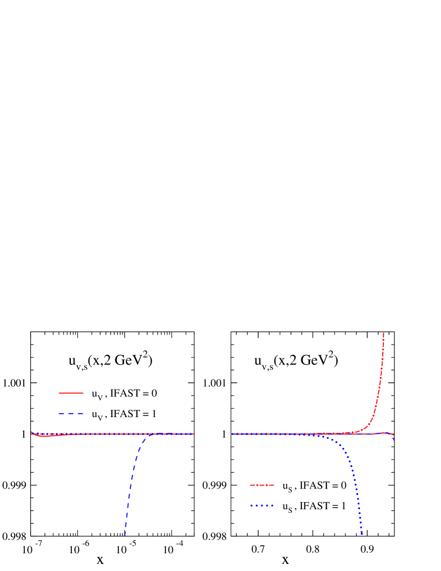
Figure 2: The up-valence and up-sea distributions at the initial scale (4.2) obtained by the standard and fast Mellin inversions, divided by the exact $x$-space inputs in Eq. (4.2). The same four curves are shown in the left (right) part for small (large) values of $x$.

The results for the standard inversion using up to 144 moments (IFAST = 0) for this test do not show any noticeable deviations from the exact values at $10^{-6}<x<0.9$ for $u_{\rm v}$, and at $10^{-11}<x<0.8$ for $u_{\rm s}$. These ranges refer to the program’s default value $c=1.9$ of the contour abscissa in Eq. (3.2). Smaller values would improve the inversion of $u_{\rm v}$ at extremely small $x$ at the cost of worsening that of $u_{\rm s}$ at very large $x$.

The faster, but close to the end-points inevitably less reliable option using between 32 and 80 moments (IFAST = 1) can be safely employed at least for $10^{-4}\,\raisebox{-1.9919pt}{$\>\stackrel{{\scriptstyle<}}{{{\scriptstyle\sim}}}\>$}\,x\,\raisebox{-1.9919pt}{$\>\stackrel{{\scriptstyle<}}{{{\scriptstyle\sim}}}\>$}\,0.7$, where the upper limit includes the effect of the further softening of the sea-quark distributions by the evolution. In many applications the small (and anyway poorly known) distributions $xu_{\rm v}$ at smaller $x$ and $u_{\rm s}$ at larger $x$ are practically irrelevant; then the fast inversion can be used over the full range of $x$ shown in the figure.

At NNLO the present overall accuracy of the program at ‘normal’ values of $x$ is dominated by that of the parametrizations of the corresponding splitting functions and the $n_{\!f}$-matching coefficient discussed in section 3.2. An update of the NNLO benchmark results in ref. [37] with the complete three-loop splitting functions of refs. [13, 14] will be presented elsewhere [39]. For checks of tables 5 and 6 in ref. [37] the user needs to employ the previous approximations [36] instead of the routines 5.1.8 and 5.1.9. For the moment these approximations are still available as pns2mold.f and psg2mold.f .

Finally we illustrate the speed of the program. For this purpose the input (4.2) is evolved, using Eqs. (4.2) and (4.3), for variable $n_{\!f}$ to 20 scales $\mu^{2}$ and the results are Mellin-inverted at 25 values of $x$ at each scale. The chosen scales and values of $x$ are

       DATA MS / 2.0D0,  2.7D0,  3.6D0,  5.D0,   7.D0,   1.D1,
     1           1.4D1,  2.D1,   3.D1,   5.D1,   7.D1,   1.D2,
     2           2.D2,   5.D2,   1.D3,   3.D3,   1.D4,   4.D4,
     3           2.D5,   1.D6 /
       DATA XB / 1.D-8,  1.D-7,  1.D-6,
     1           1.D-5,  2.D-5,  5.D-5,  1.D-4,  2.D-4,  5.D-4,
     1           1.D-3,  2.D-3,  5.D-3,  1.D-2,  2.D-2,  5.D-2,
     2           1.D-1, 1.5D-1,  2.D-1,  3.D-1,  4.D-1,  5.D-1,
     3           6.D-1,  7.D-1,  8.D-1,  9.D-1 / .

The whole calculation, including the input initialization but excluding the general initialization, is then repeated 200 times. Thus we perform precisely $10^{\,5}$ calls of XPARTON. The times (in seconds) required for this computation on a 2.0 GHz Pentium-IV processor are listed below for various values of NPORD, IMODEV and IFAST (defined in section 4.1). The value of the latter parameter is given after the name of the compiler. We have used the GNU compiler g77 (version 3.2-36) with -O2 and the (non-commercial) ‘Intel Fortran Compiler 8.0 for Linux’ ifort with -xW (optimization with -O2 is the default for ifort).

Type of evolution	g77,0	g77,1	ifort,0	ifort,1
LO	7.8	4.3	2.5	1.4
IMODEV=0, NLO	8.2	4.5	2.7	1.5
IMODEV=0, NNLO	9.2	5.0	3.2	1.8
IMODEV=1, NLO	10.7	5.8	3.8	2.1
IMODEV=1, NNLO	11.3	6.2	4.4	2.4

Thus roughly $10^{\,4}$ to $10^{\,5}$ Mellin inversions of the complete set of partons can be performed per second under the above conditions, depending on the initialization parameters and the available compiler. As expected, the evolution becomes somewhat slower with increasing order, and the iterative solutions (involving high orders of the evolution matrices $U$) are slower than the truncated evolution.

7 Summary and outlook

We have presented the fast, flexible and accurate Fortran package QCD-Pegasus solving the evolution equations for the unpolarized and polarized parton distributions of hadrons in perturbative QCD. The code is designed such that the program is relatively fastest when this is most needed, viz in large repetitive computations like fits of the initial distributions or error analyses according to refs. [40, 41, 42]. In standard applications, the user needs to interact with only very few top-level routines which communicate the evolution parameters and initial distributions to, and the results of the evolution from the lower-level routines actually performing the underlying evolution in Mellin-$N$ space.

The full potential of the $N$-space approach is realized once not only the parton evolution, but also the convolutions with the partonic cross sections (coefficient functions) are performed (as multiplications of the moments) before Mellin-inverting back to $x$-space. Doing this poses no problems if the coefficient functions are known (to a sufficient accuracy) in a form facilitating the calculation of their complex-$N$ moments. Even if this is not the case — for example, if coefficient functions are only known via an $x$-space Monte-Carlo programs including experimental cuts — there are efficient methods to proceed in $N$-space, see ref. [43] and especially refs. [44, 45]. Sample routines for the latter procedure will be presented elsewhere for representative observables in $ep$ and $pp/p\bar{p}$ scattering. The user can then implement the processes he or she is interested in along these lines. QCD-Pegasus can of course also be used efficiently within ‘normal’ $x$-space analyses.

If additional routines are included to deal with the additional ‘pointlike’ solution, the program can also be used for the QCD evolution of the parton distributions of the photon. These routines largely exist, but have not been included in this first public version of the program. An even easier extension would be the evolution of also ‘timelike’ distributions (fragmentation functions) of effectively massless partons. Considerably larger modifications would be required to include other (hypothetical) light coloured particles like a light gluino which would lead to a enlarged $3\times 3$ flavour-singlet sector. This extension was actually present in an earlier incarnation of this program, see ref. [46], but has not been pursued anymore since the light-gluino window is now generally considered closed.

The code of QCD-Pegasus can be obtained by downloading the source of this article from the hep-ph preprint archive. Relevant changes of the code, if required, will be communicated by replacing the article in this archive. The program is distributed under the GNU public license, with the obvious additional requirement that scientific publications (including preprints) which have been prepared using the present code, or a modified version of it, should include a reference to the present article. The author can be reached by electronic mail for bug reports, comments and questions.

Acknowledgments

I am grateful to M. Botje, S. Moch and W. Vogelsang for critically reading the text. This work was supported by the Dutch Foundation for Fundamental Research of Matter (FOM).

References

- [1] M. Miyama, S. Kumano, Comput. Phys. Commun. 94 (1996) 185, hep-ph/9508246
- [2] M. Hirai, S. Kumano and M. Miyama, Comput. Phys. Commun. 108 (1998) 38, hep-ph/9707220
-
[3]
A. Ouraou, Ph. D. thesis, Université de Paris-XI (1988),
M. Virchaux, Ph. D. thesis, Université de Paris-VII (1988),
M.A.J. Botje, Zeus Note 97-066, available at www.nikhef.nl/user/h24/qcdnum - [4] S. Weinzierl, Comput. Phys. Commun. 148 (2002) 314, hep-ph/0203112
- [5] W. Furmanski and R. Petronzio, Z. Phys. C11 1982) 293
- [6] M. Glück, E. Reya and A. Vogt, Z. Phys. C48 (1990) 471
- [7] O.V. Tarasov, A.A. Vladimirov, and A.Y. Zharkov, Phys. Lett. 93B (1980) 429
- [8] S.A. Larin and J.A.M. Vermaseren, Phys. Lett. B303 (1993) 334, hep-ph/9302208
- [9] T. van Ritbergen, J. Vermaseren and S. Larin, Phys. Lett. B400 (1997) 379, hep-ph/9701390
- [10] M. Abramowitz and I.A. Stegun (eds.), Handbook of Mathematical Functions, 9th printing, Dover (New York) 1974, section 25
- [11] S. Eidelman et al. [Particle Data Group Collaboration], Phys. Lett. B592 (2004) 1
- [12] K. G. Chetyrkin, B. A. Kniehl and M. Steinhauser, Phys. Rev. Lett. 79 (1997) 2184, hep-ph/9706430
- [13] S. Moch, J. Vermaseren and A. Vogt, Nucl. Phys. B688 (2004) 101, hep-ph/0403192
- [14] A. Vogt, S. Moch and J. Vermaseren, Nucl. Phys. B691 (2004) 129, hep-ph/0404111
- [15] W. L. van Neerven and A. Vogt, Nucl. Phys. B603 (2001) 42, hep-ph/0103123
- [16] J. Blümlein, S. Riemersma, M. Botje, C. Pascaud, F. Zomer, W. L. van Neerven and A. Vogt, Proceedings of the workshop Future Physics at HERA, DESY, Hamburg 1995/96, eds. G. Ingelman, A. De Roeck, R. Klanner (DESY 1996), p. 23; hep-ph/9609400
- [17] R.K. Ellis, Z. Kunszt and E.M. Levin, Nucl. Phys. B420 (1994) 517 [Erratum-ibid. B433 (1995) 498]
- [18] J. Blümlein and A. Vogt, Phys. Rev. D58 (1998) 014020, hep-ph/9712546
- [19] S. Catani, D. de Florian, G. Rodrigo and W. Vogelsang, hep-ph/0404240
- [20] S. A. Larin, T. van Ritbergen and J. A. M. Vermaseren, Nucl. Phys. B438 (1995) 278, hep-ph/9411260
- [21] M. Buza, Y. Matiounine, J. Smith and W. L. van Neerven, Eur. Phys. J. C1 (1998) 301, hep-ph/9612398
- [22] R. Courant and D. Hilbert, Methoden der Mathematischen Physik, Springer Verlag (Berlin) Bd. 1, 1924; Methods of Mathematical Physics, Interscience (New York) Vol. 1, 1953
- [23] D. A. Kosower, Nucl. Phys. B506 (1997) 439, hep-ph/9706213
- [24] A. Gonzalez-Arroyo, C. Lopez and F.J. Yndurain, Nucl. Phys. B153 (1979) 161
- [25] G. Curci, W. Furmanski and R. Petronzio, Nucl. Phys. B175 (1980) 27
- [26] E.G. Floratos, C. Kounnas and R. Lacaze, Nucl. Phys. B192 (1981) 417
- [27] M. Abramowitz and I.A. Stegun (eds.), Handbook of Mathematical Functions, 9th printing, Dover (New York) 1974, section 6
- [28] A. Devoto and D. W. Duke, Riv. Nuovo Cim. 7N6 (1984) 1
- [29] J. Blümlein and S. Kurth, Phys. Rev. D60 (1999) 014018, hep-ph/9810241
- [30] J. Blümlein, Comput. Phys. Commun. 133 (2000) 76, hep-ph/0003100
- [31] R. Mertig and W.L. van Neerven, Z. Phys. C70 (1996) 637
- [32] W. Vogelsang, Phys. Rev. D54 (1996) 2023, hep-ph/9512218
- [33] W. Vogelsang, Nucl. Phys. B475 (1996) 47, hep-ph/9603366
- [34] M. Glück, E. Reya, M. Stratmann and W. Vogelsang, Phys. Rev. D5 (1996) 4775, hep-ph/9508347
- [35] J.A.M. Vermaseren, Int. J. Mod. Phys. A14 (1999) 2037, hep-ph/9806280
- [36] W. L. van Neerven and A. Vogt, Phys. Lett. B490 (2000) 111, hep-ph/0007362
- [37] G. Salam and A. Vogt, in the QCD/SM Working Group Report of the workshop Physics at TeV Colliders, Les Houches, May 2001; hep-ph/0204316, section 1.3
- [38] CTEQ6 J. Pumplin, D.R. Stump, J. Huston, H.L. Lai, P. Nadolsky and W.K. Tung, JHEP 0207 (2002) 012, hep-ph/0201195
- [39] G. Salam and A. Vogt, in preparation
- [40] W.T. Giele and S. Keller, Phys. Rev. D58 (1998) 094023, hep-ph/9803393
- [41] W.T. Giele, S.A. Keller and D.A. Kosower, hep-ph/0104052
- [42] S. Alekhin, M. Botje, W. Giele, J. Pumplin and F. Olness, in the QCD/SM Working Group Report of the workshop Physics at TeV Colliders, Les Houches, May 2001; hep-ph/0204316, section 1.1
- [43] Ch. Berger, D. Graudenz, M. Hampel and A. Vogt, Z. Phys. C70 (1996) 77, hep-ph/9506333
- [44] D. A. Kosower, Nucl. Phys. B520 (1998) 263, hep-ph/9708392
- [45] M. Stratmann and W. Vogelsang, Phys. Rev. D64 (2001) 114007, hep-ph/0107064
- [46] R. Rückl and A. Vogt, Z. Phys. C64 (1994) 431, hep-ph/9404355