A New Parametrization of the Neutrino Mixing Matrix

Abstract

The neutrino mixing matrix is expanded in powers of a small parameter $\lambda$, which approximately equals to 0.1. The meaning of every order of the expansion is discussed respectively, and the range of $\lambda$ is carefully calculated. We also present some applications of this new parametrization, such as to the expression of the Jarlskog parameter $J$, in which the simplicities and advantages of this parametrization are shown.

,

In recent years, there have been abundant experimental data strongly suggesting the mixing of different generations of neutrinos, just analogous to that of quarks. The K2K [1] and Super-Kamiokande [2] experiments indicated that the atmospheric neutrino anomaly is due to the $\nu_{\mu}$ to $\nu_{\tau}$ oscillation with almost the largest mixing angle of $\theta_{atm}\approx 45^{\circ}$. The KamLAND [3] and SNO [4] experiments told us that the solar neutrino deficit was caused by the oscillation from $\nu_{e}$ to a mixture of $\nu_{\mu}$ and $\nu_{\tau}$ with a mixing angle approximately of $\theta_{sol}\approx 34^{\circ}$. On the other hand, the non-observation of the $\overline{\nu}_{e}$ to $\overline{\nu}_{e}$ oscillation in the CHOOZ [5] experiment showed that the mixing angle $\theta_{chz}$ is smaller than $3^{\circ}$ at the best fit point [6, 7].

These experiments not only confirmed the oscillations of neutrinos, but also measured the mass-squared differences of the neutrino mass eigenstates (the allowed ranges at 3$\sigma$) [6], $1.4\times 10^{-3}eV^{2}<\Delta m_{atm}^{2}=|m_{3}^{2}-m_{2}^{2}|<3.3\times 10^{-3}eV^{2}$, and $7.3\times 10^{-5}eV^{2}<\Delta m_{sol}^{2}=|m_{2}^{2}-m_{1}^{2}|<9.1\times 10^{-5}eV^{2}$, where $\pm$ correspond to the normal and inverted schemes respectively.

Like the Cabibbo-Kobayashi-Maskawa (CKM) [8, 9] matrix for quark mixing, the neutrino mixing matrix is described by the unitary Maki-Nakawaga-Sakata (MNS) [10] matrix $V$, which links the neutrino flavor eigenstates $\nu_{e}$, $\nu_{\mu}$, $\nu_{\tau}$ to the mass eigenstates $\nu_{1}$, $\nu_{2}$, $\nu_{3}$,

$$\left(\begin{array}[]{c}\nu_{e}\\ \nu_{\mu}\\ \nu_{\tau}\\ \end{array}\right)=\left(\begin{array}[]{ccc}V_{e1}&V_{e2}&V_{e3}\\ V_{\mu 1}&V_{\mu 2}&V_{\mu 3}\\ V_{\tau 1}&V_{\tau 2}&V_{\tau 3}\\ \end{array}\right)\left(\begin{array}[]{c}\nu_{1}\\ \nu_{2}\\ \nu_{3}\\ \end{array}\right).$$ (1)

It is always feasible to parametrize the Majorana neutrino mixing matrix as a product of a Dirac neutrino mixing matrix (with three mixing angles and a CP-violating phase) and a diagonal phase matrix (with three phase angles, and only two of them are unremovable) [11]. In a form similar to the quark mixing matrix, the neutrino mixing matrix can also be written as follows

$$V=\left(\begin{array}[]{ccc}c_{2}c_{3}&c_{2}s_{3}&s_{2}e^{-i\delta}\\ -c_{1}s_{3}-s_{1}s_{2}c_{3}e^{i\delta}&c_{1}c_{3}-s_{1}s_{2}s_{3}e^{i\delta}&s_{1}c_{2}\\ s_{1}s_{3}-c_{1}s_{2}c_{3}e^{i\delta}&-s_{1}c_{3}-c_{1}s_{2}s_{3}e^{i\delta}&c_{1}c_{2}\\ \end{array}\right)\left(\begin{array}[]{ccc}e^{i\sigma_{1}}&&\\ &e^{i\sigma_{2}}&\\ &&e^{i\sigma_{3}}\\ \end{array}\right),$$ (2)

where $s_{i}=\sin\theta_{i}$, $c_{i}=\cos\theta_{i}$ (for $i=1,2,3$), $\delta$ is the Dirac CP-violating phase and $\sigma_{1}$, $\sigma_{2}$, $\sigma_{3}$ are the Majorana CP-violating phases. If the neutrinos are of Dirac-type, the diagonal phase matrix on the right side hand of Eq. (2) can be rotated away by redefining the phases of the Dirac neutrino fields. The Dirac CP-violating phase is associated with the neutrino oscillations, CP and T violation. The Majorana CP-violating phases are associated with the neutrinoless double beta decay, and lepton-number-violating processes [12].

The three mixing angles $\theta_{atm}$, $\theta_{chz}$, and $\theta_{sol}$ are related to the three mixing angles $\theta_{1}$, $\theta_{2}$, and $\theta_{3}$, which describe the mixing between 2nd and 3rd, 3rd and 1st, 1st and 2nd generations of neutrinos. To a good degree of accuracy, $\theta_{atm}=\theta_{1}$, $\theta_{chz}=\theta_{2}$, and $\theta_{sol}=\theta_{3}$.

According to the results of the global analysis of the neutrino oscillation experiments, the elements of the modulus of the neutrino mixing matrix are summarized as follows [13]

$$|V|=\left(\begin{array}[]{ccc}0.70-0.87&0.50-0.69&<0.16\\ 0.20-0.61&0.34-0.73&0.60-0.80\\ 0.21-0.63&0.36-0.74&0.58-0.80\\ \end{array}\right).$$ (3)

Quite different from the quark mixing matrix, almost all the non-diagonal elements of the neutrino mixing matrix are large, only with the exception of $V_{e3}$. So it is unpractical to expand the matrix in powers of one of the non-diagonal elements, like the Wolfenstein parametrization of the quark mixing matrix [14]. Xing [15] has made the Wolfenstein-like parametrization for the neutrino mixing matrix, but they have to use much higher orders of the non-diagonal elements. In the quark mixing pattern, all the non-diagonal elements are small, so we may take it for granted that the mixing is a small modification to the unit matrix. But on the contrary, why could not we consider the large mixing as the common pattern, which is just the case in the neutrino mixing? So we may not expand the neutrino mixing matrix around the unit matrix.

In this letter, we will just make an expansion of the neutrino mixing matrix based on the bi-maximal mixing pattern. Since there are two mixing angles near $45^{\circ}$ ($\theta_{1}\approx 45^{\circ}$, and $\theta_{3}\approx 34^{\circ}$), the neutrino mixing matrix is not only the bi-large pattern as commonly said, but quite near the bi-maximal pattern, which reads

$$V=\left(\begin{array}[]{ccc}\sqrt{2}/2&\sqrt{2}/2&0\\ -1/2&1/2&\sqrt{2}/2\\ 1/2&-1/2&\sqrt{2}/2\end{array}\right).$$ (4)

Comparing with Eq. (3), we can make an expansion of $V$ in powers of $\lambda$, which satisfies

$$V_{e1}=\sqrt{2}/2+\lambda,$$ (5)

where $\lambda$ measures the strength of the deviation of $V_{e1}$ from the bi-maximal mixing pattern. Unlike the Wolfenstein parametrization of the quark mixing matrix, $\lambda$ here is at the diagonal element of the neutrino mixing matrix. Because $0.70<V_{e1}<0.87$, $\lambda$ is a small positive parameter, which approximately equals to 0.1, and this expansion is reasonable and will converge quickly. Because $\theta_{1}$ is quite near $45^{\circ}$, $V_{\mu 3}$ must be quite near $\sqrt{2}/2$ [1, 2]. Then we can set

$$V_{\mu 3}=\sqrt{2}/2+a\lambda^{2}.$$ (6)

Also, since $\theta_{2}$ is rather small (with the best fit point $V_{e3}=0.045$ [6]), we can set

$$V_{e3}=b\lambda^{2},$$ (7)

where $a$ and $b$ are both small parameters of order 1.

Now we will calculate all the $s_{i}$ and $c_{i}$ (for $i=1,2,3$) to the order of $\lambda^{4}$. From Eq. (7), $s_{2}=V_{e3}=b\lambda^{2}$, we have

$$c_{2}=\sqrt{1-s_{2}^{2}}=1-\frac{1}{4}b^{2}\lambda^{4}.$$ (8)

From Eq. (6), we have

$$s_{1}c_{2}=V_{\mu 3}=\sqrt{2}/2+a\lambda^{2},$$ (9)

using Eq. (8), we get

$$s_{1}=\frac{\sqrt{2}}{2}+a\lambda^{2}+\frac{\sqrt{2}}{4}b^{2}\lambda^{4}.$$ (10)

Similarly

$$c_{1} = \frac{\sqrt{2}}{2}-a\lambda^{2}-\frac{1}{4}(4\sqrt{2}a^{2}+\sqrt{2}b^{2})\lambda^{4},$$

$$c_{3} = \frac{\sqrt{2}}{2}+\lambda+\frac{\sqrt{2}}{4}b^{2}\lambda^{4},$$

$$s_{3} = \frac{\sqrt{2}}{2}-\lambda-\sqrt{2}\lambda^{2}-2\lambda^{3}-\frac{1}{4}(12\sqrt{2}+\sqrt{2}b^{2})\lambda^{4}.$$

Thus we obtain all the trigonometric functions of the three mixing angles.

Now we can get all the elements of the neutrino mixing matrix straightforwardly,

$$V_{e1} = \frac{\sqrt{2}}{2}+\lambda,$$

$$V_{e2} = \frac{\sqrt{2}}{2}-\lambda-\sqrt{2}\lambda^{2}-2\lambda^{3}-\frac{1}{2}(6\sqrt{2}+\sqrt{2}b^{2})\lambda^{4},$$

$$V_{e3} = b\lambda^{2},$$ (12)

$$V_{\mu 1} = -\frac{1}{2}+\frac{\sqrt{2}}{2}\lambda+\frac{1}{2}(2+\sqrt{2}a-b)\lambda^{2}+\frac{1}{2}(2\sqrt{2}-2a-\sqrt{2}b)\lambda^{3}$$

$$+\frac{1}{2}(6-2\sqrt{2}a+2a^{2}-\sqrt{2}ab+b^{2})\lambda^{4},$$

$$V_{\mu 2} = \frac{1}{2}+\frac{\sqrt{2}}{2}\lambda-\frac{1}{2}(\sqrt{2}a+b)\lambda^{2}-\frac{1}{2}(2a-\sqrt{2}b)\lambda^{3}$$

$$-\frac{1}{2}(2a^{2}-2b+\sqrt{2}ab)\lambda^{4},$$

$$V_{\mu 3} = \frac{\sqrt{2}}{2}+a\lambda^{2},$$ (13)

$$V_{\tau 1} = \frac{1}{2}-\frac{\sqrt{2}}{2}\lambda-\frac{1}{2}(2-\sqrt{2}a+b)\lambda^{2}-\frac{1}{2}(2\sqrt{2}+2a+\sqrt{2}b)\lambda^{3}$$

$$-\frac{1}{2}(6+2\sqrt{2}a-\sqrt{2}ab)\lambda^{4},$$

$$V_{\tau 2} = -\frac{1}{2}-\frac{\sqrt{2}}{2}\lambda-\frac{1}{2}(\sqrt{2}a+b)\lambda^{2}-\frac{1}{2}(2a-\sqrt{2}b)\lambda^{3}$$

$$+\frac{1}{2}(2b+\sqrt{2}ab-b^{2})\lambda^{4},$$

$$V_{\tau 3} = \frac{\sqrt{2}}{2}-a\lambda^{2}-\frac{1}{2}(2\sqrt{2}a^{2}+\sqrt{2}b^{2})\lambda^{4}.$$ (14)

Then we can expand the neutrino mixing matrix in powers of $\lambda$,

$$V = \left(\begin{array}[]{ccc}\frac{\sqrt{2}}{2}&\frac{\sqrt{2}}{2}&0\\ -\frac{1}{2}&\frac{1}{2}&\frac{\sqrt{2}}{2}\\ \frac{1}{2}&-\frac{1}{2}&\frac{\sqrt{2}}{2}\end{array}\right)+\lambda\left(\begin{array}[]{ccc}1&-1&0\\ \frac{\sqrt{2}}{2}&\frac{\sqrt{2}}{2}&0\\ -\frac{\sqrt{2}}{2}&-\frac{\sqrt{2}}{2}&0\end{array}\right)+\lambda^{2}\left(\begin{array}[]{ccc}0&-\sqrt{2}&b\\ \frac{1}{2}(2+\sqrt{2}a-b)&-\frac{1}{2}(\sqrt{2}a+b)&a\\ -\frac{1}{2}(2-\sqrt{2}a+b)&-\frac{1}{2}(\sqrt{2}a+b)&-a\end{array}\right)$$ (28)

$$+\lambda^{3}\left(\begin{array}[]{ccc}0&-2&0\\ \frac{1}{2}(2\sqrt{2}-2a-\sqrt{2}b)&-\frac{1}{2}(2a-\sqrt{2}b)&0\\ -\frac{1}{2}(2\sqrt{2}+2a+\sqrt{2}b)&-\frac{1}{2}(2a-\sqrt{2}b)&0\end{array}\right)+\cdots.$$

Now we will see the meaning of every order in the expansion of $V$.

1. The term of $\lambda^{0}$ is the approximation of the lowest order, where the atmospheric and solar neutrino oscillations are both of the largest mixing angles of $45^{\circ}$. We call this the bi-maximal mixing pattern.

2. The term of $\lambda^{1}$ indicates the deviation of the neutrino mixing matrix from the bi-maximal mixing pattern.

3. The term of $\lambda^{2}$ shows the effect of the CP violation. Because the CP violation is described by the element $V_{e3}$ [16], and in the terms of $\lambda^{0}$ and $\lambda^{1}$, $V_{e3}=0$, the degree of the CP violation is of the order $\lambda^{2}$ in our parametrization.

4. The term of $\lambda^{3}$ is the modification of higher order.

So in our new parametrization the terms of $\lambda^{0}$, $\lambda^{1}$, $\lambda^{2}$ show the bi-maximal mixing pattern, the deviation from the bi-maximal mixing pattern, and the CP violation effect respectively.

Next, we are going to determine the ranges of $\lambda$, $a$ and $b$. From the analysis above, we know that

$$\sin\theta_{atm} = s_{1}=\frac{\sqrt{2}}{2}+a\lambda^{2}+\frac{\sqrt{2}}{4}b^{2}\lambda^{4},$$

$$\sin\theta_{chz} = s_{2}=b\lambda^{2},$$

$$\sin\theta_{sol} = s_{3}=\frac{\sqrt{2}}{2}-\lambda-\sqrt{2}\lambda^{2}-2\lambda^{3}-\frac{1}{4}(12\sqrt{2}+\sqrt{2}b^{2})\lambda^{4}.$$ (29)

The current experimental data of these three parameters are (the allowed ranges at 3$\sigma$) [6, 7]

$$0.58 <\sin\theta_{atm}< 0.81,$$

$$0 <\sin\theta_{chz}< 0.16,$$

$$0.48 <\sin\theta_{sol}< 0.61.$$ (30)

And the best fit points are [6, 7]

$$\sin\theta_{atm} = 0.72,$$

$$\sin\theta_{chz} = 0.045,$$

$$\sin\theta_{sol} = 0.55.$$ (31)

From these three constraints, we can determine the ranges of the three parameters $\lambda$, $a$ and $b$. First, we can determine the range of $\lambda$. From Eq. (16), we have

$$0.48<\frac{\sqrt{2}}{2}-\lambda-\sqrt{2}\lambda^{2}-2\lambda^{3}-\frac{1}{4}(12\sqrt{2}+\sqrt{2}b^{2})\lambda^{4}<0.61,$$

then

$$\frac{0.28-2.83\lambda-4\lambda^{2}-5.66\lambda^{3}-12\lambda^{4}}{\lambda^{4}}<b^{2}<\frac{0.65-2.83\lambda-4\lambda^{2}-5.66\lambda^{3}-12\lambda^{4}}{\lambda^{4}}.$$

From the right part of the inequality, we have

$$0.65-2.83\lambda-4\lambda^{2}-5.66\lambda^{3}-12\lambda^{4}>0.$$ (32)

The allowed range of $\lambda$ is shown in Fig. 1, and we can see that $-0.67<\lambda<0.17$.

From the left part of the inequality, if

$$0.28-2.83\lambda-4\lambda^{2}-5.66\lambda^{3}-12\lambda^{4}>0,$$

we have $-0.62<\lambda<0.08$, which does not agree with the value of $V_{e1}$. So we must set

$$0.28-2.83\lambda-4\lambda^{2}-5.66\lambda^{3}-12\lambda^{4}<0,$$ (33)

and thus the inequality satisfies automatically. The allowed range of $\lambda$ is shown in Fig. 1, and we can see that $\lambda<-0.62$ or $\lambda>0.08$. Summarizing these results, we get $0.08<\lambda<0.17$, which is consistent with the primary estimation in Eq. (5). So it is reasonable and practical to expand the neutrino mixing matrix in powers of $\lambda$.

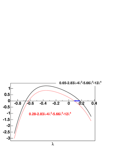
Figure 1: The allowed range of $\lambda$, the solid curve is for $0.65-2.83\lambda-4\lambda^{2}-5.66\lambda^{3}-12\lambda^{4}=0$, and the dashed curve is for $0.28-2.83\lambda-4\lambda^{2}-5.66\lambda^{3}-12\lambda^{4}=0$.

Now we can determine the range of $b$. Because $b\lambda^{2}=\sin\theta_{2}=\sin\theta_{chz}$, using Eqs. (17), (18) and $0.08<\lambda<0.17$, we have that $b=0.045/\lambda^{2}$. The range of $b$ is shown in Fig. 2, and we can see that $1.56<b<7.03$.

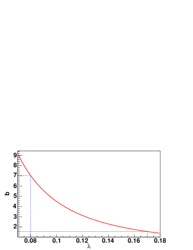
Figure 2: The range of $b$.

Similarly, in the case of $a$, $V_{\mu 3}=\sqrt{2}/2+a\lambda^{2}=s_{1}c_{2}$. Using Eq. (17) and Eq. (18), we have $0.58<s_{1}c_{2}=s_{1}\sqrt{1-s_{2}^{2}}<0.81$, with the best fit point 0.72. Thus $\sqrt{2}/2+a\lambda^{2}=0.72$, so $a=0.01/\lambda^{2}$. The range of $a$ is shown in Fig. 3, and we can see that $0.35<a<1.56$.

Figure 3: The range of $a$.

In our new parametrization, several other corresponding observable quantities associated with the elements of the neutrino mixing matrix can be expressed in relatively simple forms. From the ranges of $\lambda$, $a$ and $b$, we can determine the ranges of these observable quantities.

1. The Jarlskog parameter $J$ [17]. $J$ is the rephasing-invariant measurement of the lepton CP violation. The Majorana CP-violating phases can be removed away by redefining the phases of the Dirac fields, so only $\delta$ is associated with the CP violation. $J=\mbox{Im}(V_{e2}V_{\mu 3}V_{e3}^{\ast}V_{\mu 2}^{\ast})=s_{1}s_{2}s_{3}c_{1}c_{2}^{2}c_{3}\sin\delta$. In our parametrization, $J$ can be expressed in a very simple form (to the order of $\lambda^{4}$)

$$J=(\frac{\sqrt{2}}{2})^{4}b\lambda^{2}\sin\delta(1-4\lambda^{2}).$$ (34)

Because $s_{1}$, $s_{3}$, $c_{1}$, $c_{3}$ all have the factor $\sqrt{2}/2$, there are four $\sqrt{2}/2$ in $J$. So the degree of the lepton CP violation is suppressed four times. Again, $J$ is suppressed by the factor $b\lambda^{2}=0.045$ [6]. Using $0.08<\lambda<0.17$, $1.56<b<7.03$, we can determine the range of $J$ in Fig. 4, and we can see that $J\approx 0.00996\sim 0.01096$ (here we take $\sin\delta\sim 1$).

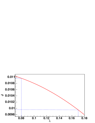
Figure 4: The range of $J$.

2. The effective Majorana mass term $\langle m\rangle_{ee}$. In the neutrinoless double beta decay, the effective Majorana mass term is defined as follows

$$\langle m\rangle_{ee}\equiv|m_{1}V_{e1}^{2}e^{2i\sigma_{1}}+m_{2}V_{e2}^{2}e^{2i\sigma_{2}}+m_{3}V_{e3}^{2}e^{2i\sigma_{3}}|,$$

where $\sigma_{1}$, $\sigma_{2}$, $\sigma_{3}$ are the Majorana CP-violating phases [12]. Using Eq. (12), we get

$$\langle m\rangle_{ee}= |\frac{1}{2}(m_{1}e^{2i\sigma_{1}}+m_{2}e^{2i\sigma_{2}})+(\sqrt{2}\lambda+\lambda^{2})(m_{1}e^{2i\sigma_{1}}-m_{2}e^{2i\sigma_{2}})$$ (35)

$$+b^{2}\lambda^{4}(m_{3}e^{2i\sigma_{3}}-m_{2}e^{2i\sigma_{2}})|.$$

We can see that the coefficients of the three terms show the influences of the three orders of $\lambda$. Only $m_{1}$ and $m_{2}$ are important to the value of $\langle m\rangle_{ee}$, and influence of $m_{3}$ almost vanish if the masses of the three mass eigenstates are nearly degenerated, because the coefficient $b^{2}\lambda^{4}$ is of $10^{-3}$.

3. The effective mass terms of neutrinos. The effective mass terms of neutrinos can be defined as follows (here we take electron neutrino for example.)

$$\langle m\rangle_{e}^{2}\equiv m_{1}^{2}|V_{e1}|^{2}+m_{2}^{2}|V_{e2}|^{2}+m_{3}^{2}|V_{e3}|^{2}.$$

Using Eq. (12), we get

$$\langle m\rangle_{e}^{2}=\frac{1}{2}(m_{1}^{2}+m_{2}^{2})-(\sqrt{2}\lambda+\lambda^{2})(m_{2}^{2}-m_{1}^{2})+b^{2}\lambda^{4}(m_{3}^{2}-m_{2}^{2}).$$ (36)

Again, the coefficients of the three terms show the influences of the three orders of $\lambda$. Noting that $\Delta m_{sol}^{2}=|m_{2}^{2}-m_{1}^{2}|$ and $\Delta m_{atm}^{2}=|m_{3}^{2}-m_{2}^{2}|$, we can rewrite Eq. (21) into

$$\langle m\rangle_{e}^{2}=m_{1}^{2}\pm[\frac{1}{2}-(\sqrt{2}\lambda+\lambda^{2})]\Delta m_{sol}^{2}\pm b^{2}\lambda^{4}\Delta m_{atm}^{2}.$$ (37)

We can see from Eq. (24) that $\langle m\rangle_{e}^{2}$ is directly related with the masses and the mass-squared differences of neutrinos. So these two kinds of different observable quantities are associated together in our parametrization. If we can separately measure $\Delta m_{atm}^{2}$, $\Delta m_{sol}^{2}$, and $\langle m\rangle_{e}^{2}$ to a good degree of accuracy, we can fix the value of $m_{1}$, which will help us determine the absolute mass of neutrino ultimately.

In summary, although all kinds of parametrization of the neutrino mixing matrix are mathematically equivalent, and applying any of them does not have any specific physical significance, however, it is quite likely that some particular parametrization does have its usefulness and advantages in analysis of various experimental data. Furthermore, we can express other observable quantities in a simple and transparent way, and can link several different kinds of observable quantities together. This is the purpose of our new parametrization, and we hope that this new parametrization will be useful in the phenomenology of neutrino physics.

Acknowledgments

We are grateful for the discussions with Prof. Zhizhong Xing. This work is partially supported by National Natural Science Foundation of China under Grant Numbers 10025523 and 90103007.

References

[1]
K2K Collaboration, M.H. Ahn, et al., Phys. Rev. Lett. 90 (2003) 041801.
[2]
C.K. Jung, C. McGrew, T. Kajita, T. Mann,
Anna. Rev. Nucl. Part. Sci. 51 (2001) 451.
[3]
KamLAND Collaboration, K. Eguchi, et al., Phys. Rev. Lett. 90 (2003) 021802.
[4]
SNO Collaboration, Q.R. Ahmad, et al., Phys. Rev. Lett. 89 (2002) 011301;
SNO Collaboration, Q.R. Ahmad, et al., Phys. Rev. Lett. 89 (2002) 011302.
[5]
CHOOZ Collaboration, M. Apollonio, et al.,
Phys. Lett. B 420 (1998) 397;
Palo Verde Collaboration, F. Boehm, et al., Phys. Rev. Lett. 84 (2000) 3764.
[6]
M. Maltoni, T. Schwetz, M.A. Tortola, J.W.F. Valle,
hep-ph/0405172, New J. Phys. 6 (2004) 122.
[7]
G. Altarelli, F. Feruglio, hep-ph/0405048, New J. Phys. 6
(2004) 106.
[8]
N. Cabibbo, Phys. Rev. Lett. 10 (1963) 531.
[9]
M. Kobayashi, T. Maskawa, Prog. Theor.
Phys. 149 (1973) 652.
[10]
Z. Maki, M. Nakawaga, S. Sakata, Prog. Theor.
Phys. 28 (1962) 870.
[11]
J. Schechter, J.W.F. Valle, Phys. Rev. D 22 (1980) 2227;
S.M. Bilenky, J. Hosek, S.T. Petsov,
Phys. Lett. B 94 (1980) 495.
[12]
J. Schechter, J.W.F. Valle, Phys. Rev. D 23 (1981) 1666;
J. Schechter, J.W.F. Valle, Phys. Rev. D 24 (1981) 1883;
J. Schechter, J.W.F. Valle, Phys. Rev. D 25 (1982) 283.