Gravitino Dark Matter in the CMSSM
and Implications for Leptogenesis and the LHC

Abstract:

In the framework of the CMSSM we study the gravitino as the lightest supersymmetric particle and the dominant component of cold dark matter in the Universe. We include both a thermal contribution to its relic abundance from scatterings in the plasma and a non–thermal one from neutralino or stau decays after freeze–out. In general both contributions can be important, although in different regions of the parameter space. We further include constraints from BBN on electromagnetic and hadronic showers, from the CMB blackbody spectrum and from collider and non–collider SUSY searches. The region where the neutralino is the next–to–lightest superpartner is severely constrained by a conservative bound from excessive electromagnetic showers and probably basically excluded by the bound from hadronic showers, while the stau case remains mostly allowed. In both regions the constraint from CMB is often important or even dominant. In the stau case, for the assumed reasonable ranges of soft SUSY breaking parameters, we find regions where the gravitino abundance is in agreement with the range inferred from CMB studies, provided that, in many cases, a reheating temperature $T_{\rm R}$ is large, $T_{\rm R}\sim 10^{9}\,\mbox{GeV}$. On the other side, we find an upper bound $T_{\rm R}\mathrel{\hbox to0.0pt{\lower 4.0pt\hbox{\hskip 1.0pt$\sim$}\hss}\raise 1.0pt\hbox{$<$}}5\times 10^{9}\,\mbox{GeV}$. Less conservative bounds from BBN or an improvement in measuring the CMB spectrum would provide a dramatic squeeze on the whole scenario, in particular it would strongly disfavor the largest values of $T_{\rm R}\sim 10^{9}\,\mbox{GeV}$. The regions favored by the gravitino dark matter scenario are very different from standard regions corresponding to the neutralino dark matter, and will be partly probed at the LHC.

1 Introduction

Low–energy supersymmetry (SUSY) provides perhaps the most attractive candidates for cold dark matter (CDM) in the Universe. This is because in the SUSY spectrum several new massive particles appear, some of which carry neither electric nor color charges. The lightest among them (the lightest SUSY partner, or the LSP) can then be neutral and either absolutely stable by virtue of some discrete symmetry, like $R$–parity, or very long–lived, much longer than the age of the Universe, and thus effectively stable. A particularly well–known and attractive example of such a weakly–interacting massive particle (WIMP) is the lightest neutralino. In recent years, however, there has been also a renewed interest in the two alternative well–motivated SUSY candidates for WIMPs and CDM, namely the gravitino and the axino.

The spin–$3/2$ gravitino acquires its mass from spontaneous breaking of local SUSY, or supergravity. Since its interactions with ordinary matter are typically strongly suppressed by an inverse square of the (reduced) Planck mass, cosmological constraints become an issue [1]. Early on it was thought that, with a primordial population of gravitinos decoupling very early, if stable, they had to very light, below some $\mathrel{\hbox to0.0pt{\lower 4.0pt\hbox{\hskip 1.0pt$\sim$}\hss}\raise 1.0pt\hbox{$<$}}1\,\mbox{keV}$ [2], in order not to overclose the Universe, or otherwise very heavy, $\mathrel{\hbox to0.0pt{\lower 4.0pt\hbox{\hskip 1.0pt$\sim$}\hss}\raise 1.0pt\hbox{$>$}}10\,\mbox{TeV}$ [3], so that they could decay before the period of BB nucleosynthesis (BBN). With inflation these bounds disappear [4, 5] but other problems emerge when gravitinos are re–generated after reheating. If the gravitino is not the LSP, it decays late ($\sim 10^{8}\sec$) into the LSP (say the neutralino) and an energetic photon which can distort the abundances of light elements produced during BBN, for which there is a good agreement of calculations with direct observations and with CMB determinations. Since the number density of gravitinos is directly proportional to the reheating temperature $T_{\rm R}$, this leads to an upper bound of $T_{\rm R}<10^{6-8}\,\mbox{GeV}$ [4, 5, 6, 7, 8, 9] (for recent updates see, e.g., [10, 11]). On the other hand, when the gravitino is the LSP and stable, ordinary sparticles can decay into it and an energetic photon. A combination of this and the overclosure argument ($\Omega_{\widetilde{G}}h^{2}<1$) leads in this case to an upper bound $T_{\rm R}\mathrel{\hbox to0.0pt{\lower 4.0pt\hbox{\hskip 1.0pt$\sim$}\hss}\raise 1.0pt\hbox{$<$}}10^{9}\,\mbox{GeV}$ [6, 12].

Because of many similarities, for comparison we comment here on axinos as DM. The axino is a fermionic superpartner of the axion in supersymmetric models with the Peccei–Quinn (PQ) mechanism implemented for solving the strong CP problem [13]. Axino interactions with ordinary matter are suppressed by $1/f_{a}^{2}$, where $f_{a}\sim 10^{11}\,\mbox{GeV}$ is the PQ scale. In many models the axino mass is not directly determined by a SUSY breaking scale $M_{\rm SUSY}$, in contrast to the neutralino and the gravitino, and therefore the axino can naturally be the LSP. Without inflation the axino has to be light ($\mathrel{\hbox to0.0pt{\lower 4.0pt\hbox{\hskip 1.0pt$\sim$}\hss}\raise 1.0pt\hbox{$<$}}1\,\mbox{keV}$) and thus warm DM [14, 15, 16, 17, 18]. Otherwise it can naturally be a cold DM [19, 17, 20], so long as $T_{\rm R}\mathrel{\hbox to0.0pt{\lower 4.0pt\hbox{\hskip 1.0pt$\sim$}\hss}\raise 1.0pt\hbox{$<$}}10^{4-5}\,\mbox{GeV}$. Constraints from Big Bang Nucleosynthesis (BBN) on axino CDM are relatively weak since NLSP decays to them typically take place before BBN. See [21] for an improved treatment of thermal production of axinos at $T_{\rm R}\mathrel{\hbox to0.0pt{\lower 4.0pt\hbox{\hskip 1.0pt$\sim$}\hss}\raise 1.0pt\hbox{$>$}}10^{5}\,\mbox{GeV}$.

For both the gravitinos and the axinos, despite their typical interaction strengths being so much weaker than electroweak, their relic abundance can still be of the favored value of $\sim 0.1$. This is because they can be efficiently produced in a class of thermal production (TP) processes involving scatterings and decays of particles in the primordial plasma, depending on $T_{\rm R}$. Alternatively, in a non–thermal production (NTP) class of processes, the next–to–lightest supersymmetric particle (NLSP) first freezes out and next decays to the axino or gravitino. These mechanisms are supposed to re–generate the relics, after their primordial population has been diluted by a proceeding period of inflation.

In TP, gravitino (or, alternatively, axino) production proceeds predominantly through ten classes of processes involving gluinos [5, 12]. In four of them, a logarithmic singularity appears due to a $t$–channel exchange of a massless gluon which can be regularized by introducing a thermal gluon mass [5, 12]. A full result for the singular part was obtained in [22]. In [23] a resumed gluon propagator was used to obtain the finite part of the production rate, and an updated expression for the relic abundance $\Omega^{\rm TP}_{\widetilde{G}}h^{2}$ of gravitinos generated via TP, valid at high $T_{\rm R}$, was given

$$\Omega^{\rm TP}_{\widetilde{G}}h^{2}\simeq 0.2\left(\frac{T_{\rm R}}{10^{10}\,\mbox{GeV}}\right)\left(\frac{100\,\mbox{GeV}}{m_{\widetilde{G}}}\right)\left(\frac{m_{\tilde{g}}(\mu)}{1\,\mbox{TeV}}\right)^{2},$$ (1)

where $m_{\tilde{g}}(\mu)$ above is the running gluino mass. In [22, 23] it was argued that, for natural ranges of the gluino and the gravitino masses, one can have $\Omega^{\rm TP}_{\widetilde{G}}h^{2}\sim 0.1$ at $T_{\rm R}$ as high as $10^{9-10}\,\mbox{GeV}$. Such high values of $T_{\rm R}$ are essential for thermal leptogenesis [24, 25], with a lower limit of $T_{\rm R}>2\times 10^{9}\,\mbox{GeV}$ [26].

The issue of gravitino relics generated in NTP processes and associated constraints was recently re–examined in detail in  [27, 28, 29, 30] and in [31]. Since all the NLSPs decay into gravitinos, in this case

$$\Omega^{\rm NTP}_{\widetilde{G}}h^{2}=\frac{m_{\widetilde{G}}}{m_{{\rm NLSP}}}\Omega_{\rm NLSP}h^{2},$$ (2)

where $\Omega^{\rm NTP}_{\widetilde{G}}h^{2}$ is the NTP contribution to the gravitino relic abundance and $\Omega_{\rm NLSP}h^{2}$ would have been the relic abundance of the NLSP if it had remained stable. Note that $\Omega^{\rm NTP}_{\widetilde{G}}h^{2}$ grows with $m_{\widetilde{G}}$.

In grand–unified SUSY frameworks, like the popular Constrained Minimal Supersymmetric Standard Model (CMSSM) [32], which encompasses a class of unified models where at the GUT scale gaugino soft masses unify to $m_{1/2}$ and scalar ones unify to $m_{0}$, one often finds that the relic abundance of the neutralino (or the stau) is actually significantly larger than $0.1$. One therefore in general cannot neglect the contribution from the NTP mechanism, unless $m_{\widetilde{G}}$ is rather small. In this case, however, at high $T_{\rm R}\sim 10^{9}\,\mbox{GeV}$, TP contribution is likely to play a role, since $\Omega^{\rm TP}_{\widetilde{G}}h^{2}\propto{T_{\rm R}/m_{\widetilde{G}}}$. Clearly, in general both TP and NTP must be simultaneously considered.

In [30] NTP of gravitinos was considered in an effective low–energy SUSY scenario. The relic abundance of gravitinos from NTP via neutralino, stau (which had already been examined in gauge–mediated SUSY breaking schemes in [33]) and sneutrino NLSP decays was however only crudely approximated and that from TP was not included at all. A weak constraint $\Omega^{\rm NTP}_{\widetilde{G}}h^{2}\mathrel{\hbox to0.0pt{\lower 4.0pt\hbox{\hskip 1.0pt$\sim$}\hss}\raise 1.0pt\hbox{$<$}}0.1$ (rather than $\Omega^{\rm NTP}_{\widetilde{G}}h^{2}\sim 0.1$) was assumed. On the other hand, constraints from BBN were treated with much care. Typically, lifetimes for NLSP decays into gravitinos are $\sim 10^{8}\sec$ in which case constraints from electromagnetic fluxes are particularly important. Nevertheless, hadronic showers, which in the past were thought to be important only for lifetimes $\mathrel{\hbox to0.0pt{\lower 4.0pt\hbox{\hskip 1.0pt$\sim$}\hss}\raise 1.0pt\hbox{$<$}}10^{4}\sec$, must also be included in considering particle decays in late times, since they provide additional strong constraints. In the case of light gravitinos in gauge–mediated SUSY breaking schemes this constraint was applied in [34] and in the case of CDM gravitinos in [29, 30]. Furthermore, in [29, 30] substantial constraints on the SUSY parameter space were derived from a requirement of not distorting the CMB blackbody spectrum by energetic photons [1, 5].

NTP of gravitinos in the framework of the CMSSM was examined in [31]. Constraints from electromagnetic showers were applied, but not from hadronic ones. Nor was the constraint from CMB applied. Gravitino abundance from NTP was computed much more accurately than in [27, 28, 29, 30]. On the other hand, similarly to [27, 28, 29, 30], only cosmologically allowed regions $\Omega^{\rm NTP}_{\widetilde{G}}h^{2}\mathrel{\hbox to0.0pt{\lower 4.0pt\hbox{\hskip 1.0pt$\sim$}\hss}\raise 1.0pt\hbox{$<$}}0.1$ were delineated but not cosmologically favored ones of $\Omega^{\rm NTP}_{\widetilde{G}}h^{2}\simeq 0.1$. For the assumed ranges of parameters some regions were found where $\Omega^{\rm NTP}_{\widetilde{G}}h^{2}$ was not excessively large, but actually too low. (In [31] it was also noted that any possible stau NLSP asymmetry would be washed away by stau pair–annihilation into tau pairs.) As we will show later, unlike the authors of [31], in the CMSSM at large values of $m_{1/2}$ (beyond those considered in [31]) we have found cosmologically favored regions of $\Omega^{\rm NTP}_{\widetilde{G}}h^{2}\simeq 0.1$.

A question arises for which values of SUSY parameters, as well as $T_{\rm R}$, the combination of gravitino yields from both TP and NTP gives $\Omega_{\widetilde{G}}h^{2}\sim 0.1$ in unified SUSY schemes. In this paper we investigate this issue within the CMSSM, which is a model of much interest. We assume no specific underlying supergravity model and treat $m_{\widetilde{G}}$ as a free parameter. In the CMSSM soft masses are assumed to be generated via a gravity–mediated SUSY breaking mechanism, in which case $m_{1/2}$, $m_{0}$ and $m_{\widetilde{G}}$ can be in the  GeV to  TeV range, and we need to ensure that the gravitino is the LSP. We compute the relic abundance of gravitinos with high accuracy which matches present observational precision of CDM abundance determinations. In evaluating $\Omega^{\rm TP}_{\widetilde{G}}h^{2}$ we follow [23], while $\Omega^{\rm NTP}_{\widetilde{G}}h^{2}$ is determined by the yield of the NLSP which we compute numerically, following our own calculation (without partial wave expansion), as described below. We apply constraints from both the electromagnetic and from the hadronic fluxes and from CMB spectrum, as well as the usual constraints from collider and non–collider SUSY searches. We concentrate on the largest $T_{\rm R}\sim 10^{9}\,\mbox{GeV}$ but also consider the region of low $T_{\rm R}$ where NTP dominates.

Before proceeding, we should note that there are other possible gravitino production mechanisms, e.g. via inflaton decay or during preheating [35, 36], but they are much more model dependent and not necessarily efficient [37]. Alternatively, gravitinos may be produced from decays of moduli fields [38]. In this paper, we do not include these effects.

We further assume $R$–parity conservation, both for simplicity and because otherwise it is hard to understand why weak universality works so well. However, it is worth remembering that in the case of such super–weakly interacting relics as the axino or the gravitino, $R$–parity is not really mandatory, unlike in the case of the neutralino WIMP. Indeed, the suppression provided by the PQ or Planck scale is often sufficient to ensure effective stability of such relics on cosmological time scales even when $R$–parity breaking terms are close to their present upper bounds. Indeed, in the case of the axino CDM, a tiny amount of its decay products into $e^{+}e^{-}$ pairs has been proposed as an interesting way of explaining an apparent INTEGRAL anomaly [39].

In the following, we will first summarize our procedures for computing $\Omega_{\widetilde{G}}h^{2}$ via both TP and NTP. Then we will list NLSP decay modes into gravitinos, and discuss constraints on the CMSSM parameter space, in particular those from BBN and CMB. Finally, we will discuss implications of our results for thermal leptogenesis and for SUSY searches at the LHC.

2 Gravitino Relic Abundance

The present relic abundance of any stable, massive relics ($\chi$, $\tilde{\tau}$, $\tilde{a}$, $\widetilde{G}$, …) produced either thermally or non-thermally is related to their yield as

$$Y=3.7\times 10^{-12}\left(\frac{100\,\mbox{GeV}}{m}\right)\left(\frac{\Omega h^{2}}{0.1}\right).$$ (3)

where $m$ is the mass of the relic particle.

2.1 TP

The yield of massive relics generated through TP processes can be obtained by integrating the Boltzmann equation with both scatterings and decays of particles in the expanding plasma [40]. In the case of the gravitino LSP, dominant contributions come from 2–body processes involving gluinos [5, 12, 22, 23]. These are given by a dimension–5 part of the Lagrangian describing gravitino interactions with gauge bosons and gauginos. For the ten classes of scattering processes the cross section, at large energies, has the form

$$\sigma(s)\propto\frac{1}{M_{\rm P}^{2}}\left(1+\frac{m_{\tilde{g}}^{2}}{3m_{\widetilde{G}}^{2}}\right),~{}~{}~{}~{}~{}~{}~{}~{}~{}~{}~{}~{}~{}s\gg M_{\rm SUSY},$$ (4)

where $M_{\rm P}=1/\sqrt{8\pi G_{N}}=2.4\times 10^{18}\,\mbox{GeV}$ is the reduced Planck mass.

In actual computations we solve the Boltzmann equation numerically by following the usual steps described, e.g., in [23, 17], and use the expression (44) of [23] for the sum of soft and hard contributions to the collision terms.

We do not include gluino decays into gravitinos which, like in the case of axino LSP, would only become important at $T_{\rm R}\sim m_{\tilde{g}}$ [12, 17]. This is because we concentrate on large $T_{\rm R}\sim 10^{9}\,\mbox{GeV}$ which are relevant for models of thermal leptogenesis.

2.2 NTP

In computing the relic abundance of gravitinos generated through NTP processes we first compute their yield after freezeout. In the CMSSM in most cases the NLSP is either the (bino–like) neutralino or the lighter stau. In the case of the neutralino, we include exact cross sections for all the tree–level two–body neutralino processes of pair–annihilation [42, 43] and coannihilation with the charginos, next–to–lightest neutralinos [44] and sleptons [45]. This allows us to accurate compute the yield and $\Omega_{\chi}h^{2}$ in the usual case when the lightest neutralino is the LSP. We further extend the above procedure to the case where the NLSP is the lightest stau ${\tilde{\tau}}_{1}$ (a lower mass eigenstate of $\tilde{\tau}_{R}$ and $\tilde{\tau}_{L}$). We include all slepton–slepton annihilation and slepton–neutralino coannihilation processes. In both cases we numerically solve the Boltzmann equation for the NLSP yield and use exact (co)annihilation cross sections which properly take into account resonance and new final–state threshold effects. The procedure has been described in detail in [46] and was recently applied to the case of axino LSP [47].

3 NLSP Decays into Gravitinos

Once the NLSPs freeze out from thermal plasma at $t\sim 10^{-12}\sec$, their comoving number density remains basically constant until they start decaying into gravitinos at late times $t\sim 10^{4}-10^{8}\sec$ (so long as $m_{\widetilde{G}}\mathrel{\hbox to0.0pt{\lower 4.0pt\hbox{\hskip 1.0pt$\sim$}\hss}\raise 1.0pt\hbox{$>$}}0.1M_{\rm SUSY}$ which we assume here). Associated decay products generate energetic fluxes which are mostly electromagnetic (EM) but also hadronic (HAD). If too large, these will wreck havoc on the abundances of light elements. Limits on electromagnetic showers become important for $t\mathrel{\hbox to0.0pt{\lower 4.0pt\hbox{\hskip 1.0pt$\sim$}\hss}\raise 1.0pt\hbox{$>$}}10^{4}\sec$ and come mainly either from excessive deuterium destruction via $\gamma+D\rightarrow n+p$ ($10^{4}\sec\mathrel{\hbox to0.0pt{\lower 4.0pt\hbox{\hskip 1.0pt$\sim$}\hss}\raise 1.0pt\hbox{$<$}}t\mathrel{\hbox to0.0pt{\lower 4.0pt\hbox{\hskip 1.0pt$\sim$}\hss}\raise 1.0pt\hbox{$<$}}10^{6}\sec$), or production via $\gamma+{{}^{4}}{\!He}\rightarrow D+\ldots$ ($t\mathrel{\hbox to0.0pt{\lower 4.0pt\hbox{\hskip 1.0pt$\sim$}\hss}\raise 1.0pt\hbox{$>$}}10^{6}\sec$). Decay rates and branching ratios into EM radiation generated by late–decaying particles have recently been re–analyzed by Cyburt, et al., in [10]. Updated bounds on EM fluxes have been obtained on the parameter $\zeta_{X}=m_{X}n_{X}/n_{\gamma}$, where $X$ denotes the decaying particle, $n_{\gamma}$ is a number density of background photons, as a function of $X$ lifetime $\tau_{X}$, by assuming that in $X\rightarrow\widetilde{G}+\ldots$ decays associated showers are mostly electromagnetic. This is indeed the case when $X$ is either the neutralino or the stau [31, 29].

Limits from BBN on hadronic showers are stronger for $\tau\mathrel{\hbox to0.0pt{\lower 4.0pt\hbox{\hskip 1.0pt$\sim$}\hss}\raise 1.0pt\hbox{$<$}}10^{4}\sec$ but are often also important at later times [48, 49, 11, 50]. They come mainly from ${{}^{4}}{\!He}$ overproduction via $n+p\rightarrow D\rightarrow{{}^{4}}{\!He}$ for $\tau_{X}\mathrel{\hbox to0.0pt{\lower 4.0pt\hbox{\hskip 1.0pt$\sim$}\hss}\raise 1.0pt\hbox{$<$}}10^{2}\sec$, and $D$ overproduction via $n+{{}^{4}}{\!He}\rightarrow D$ at later times. Hadronic components produced in late $X$ decays into gravitinos, while much less frequent, will still lead to important constraints on the parameter space, as mentioned above, and will play an important role in our analysis. Upper limits on hadronic radiation from $X$ decays, but with somewhat stronger assumptions than in [10], have recently been re–evaluated by Kawasaki, et al., in [11].

More stringent bounds, by roughly a factor of ten, come from considering constraints from ${{}^{6}}{\!Li}$ [51] and/or from ${{}^{3}}{\!He}$ [52]. As discussed, e.g., in [29] at present both are probably still too poorly determined to be treated as robust. For this reason, and in order to remain conservative, we do not use the constraint from ${{}^{6}}{\!Li}$, unlike in [31]. Nor, like in [31], do we apply the constraint from ${{}^{3}}{\!He}$.

In order to apply bounds from BBN light element abundances on EM/HAD showers produced in association with gravitinos, we need to evaluate the relative energy $\xi^{X}_{i}$ ($i={em},\,{had}$), as defined below, which is released in NLSP decays into EM/HAD radiation. First, for each NLSP decay channel we need to know the energy $\epsilon^{X}_{i}$ transferred to EM/HAD fluxes. In decays $X\rightarrow\widetilde{G}+R+\ldots$, where $R$ collectively stands for all the particles generating either EM or HAD radiation, the total energy per NLSP decay carried by $R$ will be a fraction of $m_{X}$. This is because, at late times of relevance to $\widetilde{G}$ production, the NLSPs decay basically at rest. In 2–body decays

$$E^{X}_{tot}=\frac{m_{X}^{2}-m_{\widetilde{G}}^{2}+m_{R}^{2}}{2m_{X}},$$ (5)

where now $m_{R}$ stands for mass of $R$. Unless $m_{\widetilde{G}}$ is not much less than $m_{X}$, then, for negligible $m_{R}$, the usual approximation $E^{X}_{tot}\simeq m_{X}/2$ works well. In the case of 3– and more–body final states $E^{X}_{tot}$ as a fraction of $m_{X}$ assumes a range of values.

We also need to compute the NLSP lifetime $\tau_{X}$ and branching fractions $B^{X}_{i}$ ($i={em},\,{had}$) into EM/HAD showers. All the above quantities depend on the NLSP and (with the exception of the yield) on its decay modes and the gravitino mass. For the cases of interest ($\chi$ and ${\tilde{\tau}}_{1}$) these have been recently evaluated in detail in [29, 30] (see also [31]) and below we follow their discussion.

For the neutralino NLSP the dominant decay mode is $\chi\rightarrow\widetilde{G}\gamma$ for which the decay rate is [31, 30]

$$\Gamma\left(\chi\rightarrow\widetilde{G}\gamma\right)=\frac{|N_{11}\cos\theta_{W}+N_{12}\sin\theta_{W}|^{2}}{48\pi M_{\rm P}^{2}}\frac{m_{\chi}^{5}}{m_{\widetilde{G}}^{2}}\left(1-\frac{m_{\widetilde{G}}^{2}}{m_{\chi}^{2}}\right)^{3}\left(1+3\frac{m_{\widetilde{G}}^{2}}{m_{\chi}^{2}}\right),$$ (6)

where $\chi=N_{11}\widetilde{B}+N_{12}\widetilde{W}^{0}_{3}+N_{13}\widetilde{H}^{0}_{b}+N_{14}\widetilde{H}^{0}_{t}$. In the CMSSM the neutralino is a nearly pure bino, thus $\chi\simeq\widetilde{B}$. The decay $\chi\rightarrow\widetilde{G}\gamma$ produces mostly EM energy. Thus

$$B^{\chi}_{em} \simeq 1,$$ (7)

$$\epsilon^{\chi}_{em} = \frac{m_{\chi}^{2}-m_{\widetilde{G}}^{2}}{2m_{\chi}}$$ (8)

and the energy $\xi^{\chi}_{em}$ released into electromagnetic showers is in this case simply given by

$$\xi^{\chi}_{em}\simeq\epsilon^{\chi}_{em}B^{\chi}_{em}Y^{\chi}.$$ (9)

If kinematically allowed, the neutralino can also decay via $\chi\rightarrow\widetilde{G}Z,\widetilde{G}h,\widetilde{G}H,\widetilde{G}A$ for which the decay rates are given in [31, 30]. These processes contribute to hadronic fluxes because of large hadronic branching ratios of the $Z$ and the Higgs bosons ($B^{Z}_{had}\simeq 0.7$, $B^{h}_{had}\simeq 0.9$). In this case the energy $\xi^{\chi}_{had}$ released into hadronic showers is

$$\xi^{\chi}_{had}\simeq\left(\sum{h}\epsilon^{\chi}_{had}B^{\chi}_{had}\right)Y^{\chi}$$ (10)

where the sum goes over all hadronic decay modes,

$$\sum\epsilon^{\chi}_{had}B^{\chi}_{had}\simeq\frac{\epsilon^{\chi}_{Z}\Gamma(\chi\rightarrow\widetilde{G}Z)B^{Z}_{had}+\sum\epsilon^{\chi}_{h}\Gamma(\chi\rightarrow\widetilde{G}h)B^{h}_{had}+\epsilon^{\chi}_{q\bar{q}}\Gamma(\chi\rightarrow\widetilde{G}q\bar{q})}{\Gamma\left(\chi\rightarrow\widetilde{G}\gamma\right)+\Gamma\left(\chi\rightarrow\widetilde{G}Z\right)+\Gamma\left(\chi\rightarrow\widetilde{G}h\right)},$$ (11)

where

$$\epsilon^{\chi}_{k} \approx \frac{m_{\chi}^{2}-m_{\widetilde{G}}^{2}+m_{k}^{2}}{2m_{\chi}},\qquad\textrm{for}\ k=Z,h,H,A,$$ (12)

$$\epsilon^{\chi}_{q\bar{q}} \approx \frac{2}{3}(m_{\chi}-m_{\tilde{G}}).$$ (13)

Below the kinematic threshold for neutralino decays into $\widetilde{G}$ and the $Z$/Higgs boson, one needs to include 3–body decays with the off–shell photon or $Z$ decaying into quarks for which $B^{\chi}_{had}(\chi\rightarrow\widetilde{G}\gamma^{\ast}/Z^{\ast}\rightarrow\widetilde{G}q\bar{q})\sim 10^{-3}$ [30]. This provides a lower bound on $B^{\chi}_{had}$. At larger $m_{\chi}$ Higgs boson final states become open and we include neutralino decays to them as well.

The dominant decay mode of the stau ${\tilde{\tau}}_{1}$ is ${\tilde{\tau}}_{1}\rightarrow\widetilde{G}\tau$ for which (neglecting the tau–lepton mass) the decay width is [31, 30]

$$\Gamma\left({\tilde{\tau}}_{1}\rightarrow\widetilde{G}\tau\right)=\frac{1}{48\pi M_{\rm P}^{2}}\frac{m_{{\tilde{\tau}}_{1}}^{5}}{m_{\widetilde{G}}^{2}}\left(1-\frac{m_{\widetilde{G}}^{2}}{m_{{\tilde{\tau}}_{1}}^{2}}\right)^{4}.$$ (14)

In [28, 29, 30] it was argued that decays of staus contribute basically only to EM showers, despite the fact that a sizable fraction of tau–leptons decay into light mesons, like pions and kaons. These decay electromagnetically much faster than the typical time scale of hadronic interactions, mainly because at such late times there are very few nucleons left to interact with [28]. Thus

$$B^{{\tilde{\tau}}_{1}}_{em} \simeq 1,$$ (15)

$$\epsilon^{{\tilde{\tau}}_{1}}_{em} \approx \frac{1}{2}\frac{m_{{\tilde{\tau}}_{1}}^{2}-m_{\widetilde{G}}^{2}}{2m_{{\tilde{\tau}}_{1}}},$$ (16)

where the additional factor of $1/2$ appears because about half of the energy carried by the tau–lepton is transmitted to final state neutrinos. The energy $\xi^{{\tilde{\tau}}_{1}}_{em}$ released into electromagnetic showers is in this case

$$\xi^{{\tilde{\tau}}_{1}}_{em}\simeq\epsilon^{{\tilde{\tau}}_{1}}_{em}B^{{\tilde{\tau}}_{1}}_{em}Y^{{\tilde{\tau}}_{1}}.$$ (17)

As shown in [29], for stau NLSP, the leading contribution to hadronic showers come from 3–body decays ${{\tilde{\tau}}_{1}}\rightarrow\widetilde{G}\tau Z,\widetilde{G}\nu_{\tau}W$, or from 4–body decays ${{\tilde{\tau}}_{1}}\rightarrow\widetilde{G}\tau\gamma^{\ast}/Z^{\ast}\rightarrow\widetilde{G}\tau q\bar{q}$. The corresponding energy $\xi^{{\tilde{\tau}}_{1}}_{had}$ is

$$\xi^{{\tilde{\tau}}_{1}}_{had}\simeq\left(\sum\epsilon^{{\tilde{\tau}}_{1}}_{had}B^{{\tilde{\tau}}_{1}}_{had}\right)Y^{{\tilde{\tau}}_{1}}$$ (18)

where the sum goes over all hadronic decay modes,

$$\sum\epsilon^{{\tilde{\tau}}_{1}}_{had}B^{{\tilde{\tau}}_{1}}_{had}\simeq\frac{\epsilon^{{\tilde{\tau}}_{1}}_{Z}\Gamma({\tilde{\tau}}_{1}\rightarrow\widetilde{G}\tau Z)B^{Z}_{had}+\epsilon^{{\tilde{\tau}}_{1}}_{W}\Gamma({\tilde{\tau}}_{1}\rightarrow\widetilde{G}\nu_{\tau}W)B^{W}_{had}+\epsilon^{{\tilde{\tau}}_{1}}_{q\bar{q}}\Gamma({\tilde{\tau}}_{1}\rightarrow\widetilde{G}\tau q\bar{q})}{\Gamma\left({\tilde{\tau}}_{1}\rightarrow\widetilde{G}\tau\right)},$$ (19)

and

$$\epsilon^{{\tilde{\tau}}_{1}}_{Z}\simeq\epsilon^{{\tilde{\tau}}_{1}}_{W}\simeq\epsilon^{{\tilde{\tau}}_{1}}_{q\bar{q}}\approx\frac{1}{3}(m_{{\tilde{\tau}}_{1}}-m_{\widetilde{G}}).$$ (20)

One typically finds [30] $B^{{\tilde{\tau}}_{1}}_{had}\sim 10^{-5}-10^{-2}$ when 3–body decays are allowed and $\sim 10^{-6}$ from from 4–body decays otherwise, thus providing a lower limit on the quantity. Given such a large variation in $B^{{\tilde{\tau}}_{1}}_{had}$, the choice (20) is probably as good as any other.

4 Constraints

$\bullet$  The relic abundance

We will be mostly interested in the cases where the sum $\Omega_{\widetilde{G}}h^{2}=\Omega^{\rm TP}_{\widetilde{G}}h^{2}+\Omega^{\rm NTP}_{\widetilde{G}}h^{2}$ satisfies the $2\,\sigma$ range for non–baryonic CDM

$$0.094<\Omega_{\widetilde{G}}h^{2}<0.129,$$ (21)

which follows from combining WMAP results [53] with other recent measurements of the CMB. Larger values are excluded. Lower values are allowed but disfavored. We will also delineate regions where $\Omega^{\rm NTP}_{\widetilde{G}}h^{2}$ alone satisfies the range (21). These regions will be cosmologically favored for $T_{\rm R}\ll 10^{9}\,\mbox{GeV}$ when TP can be neglected.

$\bullet$  Electromagnetic and hadronic showers and the BBN

As stated above, bounds on electromagnetic fluxes have recently been re–evaluated and significantly improved in [10], while on hadronic ones in [11]. (A clear summary of the leading constraints can be found in [29].) As mentioned above, each analysis uses somewhat different assumptions and input parameters.

In constraining EM showers, Cyburt, et al., [10] imposed the following observational bounds on light element abundances

$$1.3\times 10^{-5} <D/H< 5.3\times 10^{-5},$$ (22)

$$0.227 <Y_{p}< 0.249,$$ (23)

$$9.0\times 10^{-11} <\left({{}^{7}}{\!Li}/{H}\right)< 2.8\times 10^{-10}.$$ (24)

In the ${{}^{4}}{\!He}$ abundance ($Y_{p}$) the error bars were taken at $2\,\sigma$.

In deriving constraints from EM showers, we impose $\xi^{X}_{em}<\left(\zeta_{X}/2\right)(n_{\gamma}/s)$ where $\zeta_{X}$ is defined above and in [10] and the factor of $n_{\gamma}/s\simeq 1/7.04$ is due to a difference in our definitions of the yield. The largest allowed values of $\zeta_{X}$, as a function of $\tau_{X}$, for the assumed abundances of $D/H+Y_{p}+{{}^{7}}{\!Li}$ can be read out of fig. 7 of [10]. We fix the baryon–to–entropy ratio $\eta$ at $6.0\times 10^{-10}$, which is consistent with the WMAP result $\eta=6.1^{+0.3}_{-0.2}\times 10^{-10}$ [54].

In constraining hadronic fluxes from NLSP decays we compare with Kawasaki, et al., [11], who used the following input

$$2.0\times 10^{-5} <D/H< 3.6\times 10^{-5},$$ (25)

$$0.228 <Y_{p}< 0.248.$$ (26)

More specifically, we impose $\xi^{X}_{had}<E_{vis}Y_{X}$ where $E_{vis}Y_{X}$ is defined in [11]. The largest allowed values of $E_{vis}Y_{X}$, as a function of $\tau_{X}$, for the assumed abundances of $D/H~{}({\rm low})+Y_{p}(IT)$ can be read out of fig. 43 of [11], for which $B_{had}=1,m_{X}=1\,\mbox{TeV}$ and the effect of photo–dissociation due to electromagnetic showers was turned off.

Note that in  [11] much less conservative error bars on $D/H$ were used than in [10]. Our constraints from HAD showers are therefore going to be accordingly somewhat more uncertain than from EM ones, despite not applying the constraint from ${{}^{7}}{\!Li}$ at all.

As we will see, the ranges of supersymmetric parameters excluded by the above constraints will strongly depend on the assumed abundances of the light elements. Below we will illustrate this point explicitely in the case of the EM showers by considering the case $\xi^{X}_{em}<E_{vis}Y_{X}$ where $E_{vis}Y_{X}$ in this case is read off from fig. 42 of [11] where $B_{had}=0$.

It would be helpful to have available in the literature bounds on the hadronic fluxes assuming more generous inputs, like (22)–(24), and to allow $B_{had}$ to vary. On the other hand, the dependence in figs. 38–43 of [11] on $m_{X}$ is rather weak.

$\bullet$  CMB

As originally pointed out in [5] and recently re–emphasized in [27, 28], late injection of electromagnetic energy may distort the frequency dependence of the CMB spectrum from its observed blackbody shape. At late times of interest, energetic photons from NLSP decays lose energy through such processes as $\gamma e^{-}\rightarrow\gamma e^{-}$ but photon number remains conserved, since other processes, like double Compton scatterings and thermal bremsstrahlung, become inefficient. As a result, the spectrum follows the Bose–Einstein distribution function

$$f_{\gamma}(E)=\frac{1}{e^{E/(kT)+\mu}-1},$$ (27)

where $\mu$ here denotes the chemical potential. The current bound is [55]

$$|\mu|<9\times 10^{-5}.$$ (28)

At decay lifetimes of $\tau_{X}\mathrel{\hbox to0.0pt{\lower 4.0pt\hbox{\hskip 1.0pt$\sim$}\hss}\raise 1.0pt\hbox{$<$}}4\times 10^{11}\,\Omega_{b}h^{2}\,\sec\simeq 8.8\times 10^{9}\sec$, where $\Omega_{b}h^{2}$ is the abundance of baryons, the bound (28) leads to a constraint on the EM energy release $\xi^{X}_{em}$ defined previously via the relation [56]

$$\mu=8.01\times 10^{2}\left[\frac{\tau_{X}}{1\sec}\right]^{1/2}e^{-(\tau_{dC}/\tau_{X})^{5/4}}\times\left(\frac{7.04\,\xi^{X}_{em}}{1\,\mbox{GeV}}\right),$$ (29)

where

$$\tau_{dC} = 1.46\times 10^{8}(T_{0}/2.7\,K)^{-12/5}(\Omega_{b}h^{2})^{4/5}(1-Y_{p}/2)^{4/5}\sec$$ (30)

$$\simeq 6.085\times 10^{6}\sec$$ (31)

and we have taken $T_{0}=2.725\,K$, $\Omega_{b}h^{2}=0.022$ and $Y_{p}=0.24$. This leads to

$$\xi^{X}_{em}< 1.59\times 10^{-8}\,e^{(\tau_{dC}/\tau_{X})^{5/4}}\left(\frac{1\sec}{\tau_{X}}\right)^{1/2}.$$ (32)

At later decay lifetimes ($\tau_{X}\mathrel{\hbox to0.0pt{\lower 4.0pt\hbox{\hskip 1.0pt$\sim$}\hss}\raise 1.0pt\hbox{$>$}}4\times 10^{11}\,\Omega_{b}h^{2}\,\sec\simeq 8.8\times 10^{9}\sec$), elastic Compton scatterings are not efficient enough to lead to the Bose–Einstein spectrum [56]. Instead, the CMB spectrum can be described by the Compton $y$ parameter, $4y=\delta\epsilon/\epsilon$ given by

$$\frac{\delta\epsilon}{\epsilon}=7.04\times\frac{c^{2}}{kT(t_{\rm eff})}\xi_{em}^{X},$$ (33)

where $T(t)$ is the CMB temperature and $t_{\rm eff}=[\Gamma(1-\beta)]^{1/\beta}\tau_{X}$, with the Gamma function $\Gamma$ for a time–temperature relation $T\propto t^{-\beta}$. In the relativistic energy dominated era in the early Universe, for $T<0.1\,\mbox{MeV}$,

$$T=1.15\times 10^{-3}\left(\frac{t}{1\sec}\right)^{-1/2}\,\mbox{GeV},$$ (34)

which gives $\beta=1/2$. Thus $t_{eff}=[\Gamma(1/2)]^{2}\tau_{X}=\pi\tau_{X}$.

The present upper limit on $y$ parameter is [57]

$$|y|<1.2\times 10^{-5}.$$ (35)

This translates into an upper bound on $\xi_{em}^{X}$

$$\xi^{X}_{em}<7.84\times 10^{-9}\left(\frac{\pi\tau_{X}}{1\sec}\right)^{-1/2}\simeq 4.42\times 10^{-9}\frac{1}{\sqrt{\tau_{X}}}.$$ (36)

Thus we can see that, at the late times $\tau_{X}\mathrel{\hbox to0.0pt{\lower 4.0pt\hbox{\hskip 1.0pt$\sim$}\hss}\raise 1.0pt\hbox{$>$}}8.8\times 10^{9}\sec$, as specified above, the constraint on the parameter space coming from the $y$ parameter is applicable while at earlier times the $\mu$–parameter constraint is applicable [56].

$\bullet$  Collider and Non–Collider Bounds

The relevant bounds from LEP are from chargino and Higgs searches [58]

$$m_{\chi_{1}^{\pm}} > 104\,\mbox{GeV},$$ (37)

$$m_{h} > 114.4\,\mbox{GeV}.$$ (38)

In addition, a good agreement of the measured $BR(B\rightarrow X_{s}\gamma)$ with a Standard Model prediction places strong constraints on potential SUSY contributions to the process, which at large Higgs VEV ratio $\tan\beta$ can be substantial. We impose [59]

$$BR(B\rightarrow X_{s}\gamma)=(3.34\pm 0.68)\times 10^{-4}.$$ (39)

Finally, we exclude cases leading to tachyonic solutions and those for which the gravitino is not the LSP.

5 Results

Mass spectra of the CMSSM are determined in terms of the usual five free parameters: the previously mentioned $\tan\beta$, $m_{1/2}$ and $m_{0}$, as well as the trilinear soft scalar coupling $A_{0}$ and ${\rm sgn}(\mu)$ – the sign of the supersymmetric Higgs/higgsino mass parameter $\mu$. For a fixed value of $\tan\beta$, physical masses and couplings are obtained by running various mass parameters, along with the gauge and Yukawa couplings, from their common values at $M_{\rm GUT}$ down to $m_{Z}$ by using the renormalization group equations. We compute the mass spectra with version 2.2 of the package SUSPECT [60].

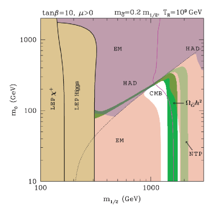
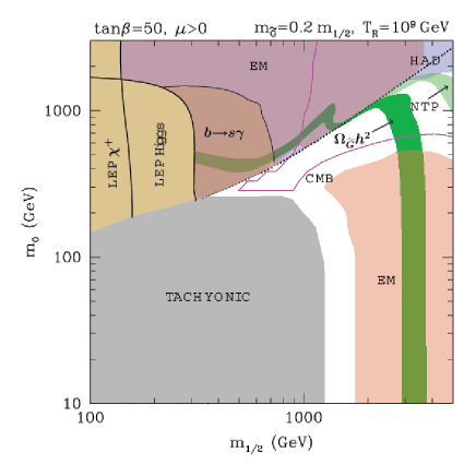
Figure 1: The plane ($m_{1/2},m_{0}$) for $\tan\beta=10$ (left window) and $\tan\beta=50$ (right window) and for $A_{0}=0$ and $\mu>0$. The light brown regions labelled “LEP $\chi^{+}$” and “LEP Higgs” are excluded by unsuccessful chargino and Higgs searches at LEP, respectively. In the right window the darker brown regions labelled “$b\to s\gamma$” and the dark grey region labelled “TACHYONIC” are also excluded. In the dark green band labelled “$\Omega_{\widetilde{G}}h^{2}$” the total relic abundance of the gravitino from both thermal and non–thermal production is in the favored range, while in the light green regions which are denoted “NTP” the same is the case for the relic abundance from NTP processes alone. Regions excluded by applying conservative bounds on electromagnetic showers from $D/H+Y_{p}+{{}^{7}}{\!Li}$ obtained with inputs (22)–(24) are denoted in orange and labelled “EM”. Regions excluded by imposing less conservative bounds on hadronic showers from $D/H+Y_{p}$ derived assuming $B_{had}=1$ and input (25)–(26) are denoted in blue and labelled “HAD”. (The overlapping EM/HAD–excluded regions appear as light violet.) A solid magenta curve labelled “CMB” delineates the region (on the side of the label) inconsistent with the CMB spectrum. The cosmologically favored (green) regions are ruled out when we apply bounds from $D/H+Y_{p}$ derived with (25)–(26) as input, as described in the text.

We present our results in the usual ($m_{1/2},m_{0}$) plane for two representative choices of $\tan\beta=10$ and $50$ and for $A_{0}=0$ and $\mu>0$. In light of the recent determinations from the Tevatron, we fix the top mass at $m_{t}=178\,\mbox{GeV}$ [61]. In fig. 1 we consider the case $m_{\widetilde{G}}=0.2m_{1/2}$ while in fig. 2 we take $m_{\widetilde{G}}=0.2m_{0}$ (top row) and $m_{\widetilde{G}}=m_{0}$ (bottom row). In both figures we fix the reheating temperature at $T_{\rm R}=10^{9}\,\mbox{GeV}$.

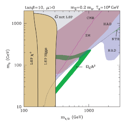
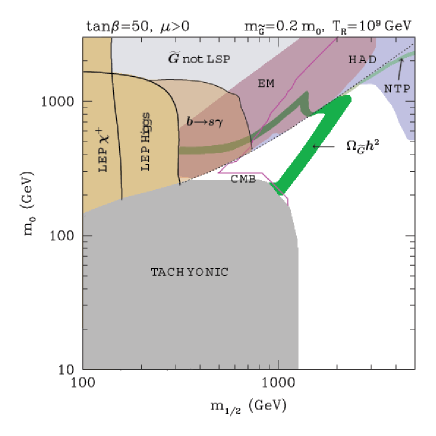
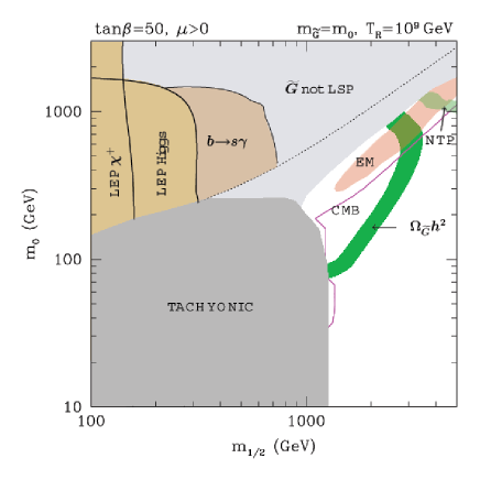
Figure 2: The same as in fig. 1 but for $m_{\widetilde{G}}=0.2m_{0}$ (top row) and $m_{\widetilde{G}}=m_{0}$ (bottom row). In the light grey areas the gravitino is not the LSP. Applying bounds from $D/H+Y_{p}$ derived with (25)–(26) as input rules out most of the cosmologically favored regions, except for small patches for $\tan\beta=50$ in the $m_{\widetilde{G}}=0.2m_{0}$ and $m_{0}$ windows, as described in the text.

To help understanding the figures, we remind the reader of some basic mass relations. The mass of the gluino is roughly given by $m_{\tilde{g}}\simeq 2.7m_{1/2}$. The mass of the lightest neutralino, which in the CMSSM is almost a pure bino, is $m_{\chi}\simeq 0.4m_{1/2}$. The lighter stau ${\tilde{\tau}}_{1}$ is dominated by ${\tilde{\tau}}_{R}$ and well above $m_{Z}$ its mass is (neglecting Yukawa contributions at large $\tan\beta$) roughly given by $m_{{\tilde{\tau}}_{1}}^{2}\simeq m_{0}^{2}+0.15m_{1/2}^{2}$. This is why at $m_{0}\ll m_{1/2}$ the stau is lighter than the neutralino while in the other case the opposite is true. The boundary between the two NLSP regions is marked in all the figures with a roughly diagonal dotted line. (In the standard scenario the region of a stable, electrically charged stau relic is thought to be ruled out on astrophysics grounds.) Regions corresponding to the lightest chargino and Higgs masses below their LEP limits, (37) and (38), respectively, are excluded. Separately marked for $\tan\beta=50$ is the region inconsistent with the measured branching ratio $BR(B\rightarrow X_{s}\gamma)$ (39). (For $\tan\beta=10$, and generally not too large $\tan\beta$, this constraint is much weaker and “hidden” underneath the above LEP bounds.) Here it is worth remembering that the constraint is derived by assuming minimal flavor violation in the squark sector – the scenario where the mass mixing in the down–type squark sector is the same as in the corresponding quark sector. However, even small perturbation of the assumption may lead to a significant relaxation (or strengthening) of the constraint from $b\rightarrow s\gamma$ [59]. At small $m_{0}$ and large $\tan\beta$ some sfermions become tachyonic. Finally, for some combinations of parameters the gravitino is not the LSP. We exclude such cases in this analysis.

Let us first concentrate on the regions where the total gravitino relic abundance $\Omega_{\widetilde{G}}h^{2}$ is consistent with the preferred range (21). In all the windows these are represented by green bands and labelled “$\Omega_{\widetilde{G}}h^{2}$”. (On the left side of the green bands $\Omega_{\widetilde{G}}h^{2}<0.094$ while on the other side $\Omega_{\widetilde{G}}h^{2}>0.129$.) Their shape looks rather different in both the neutralino and the stau NLSP regions. In the former, $\Omega_{\widetilde{G}}h^{2}$ is mostly determined by neutralino decays (NTP mechanism), except that it is relaxed relative to the case of neutralino LSP by the mass ratio $m_{\widetilde{G}}/m_{\chi}$, as in (2). (Compare with the standard neutralino LSP case in, e.g., fig. 5 of [47].) In this region of not too large $m_{1/2}$ thermal production remains (so long as $T_{\rm R}\mathrel{\hbox to0.0pt{\lower 4.0pt\hbox{\hskip 1.0pt$\sim$}\hss}\raise 1.0pt\hbox{$<$}}10^{9}\,\mbox{GeV}$) fairly inefficient, since it is proportional to $m_{\tilde{g}}$ which is still not very large there (although growing with $m_{1/2}$). In the right column of the windows where $\tan\beta=50$, one can notice a characteristic resonance due to efficient $\chi\chi$ annihilation via the pseudoscalar Higgs $A$ exchange.

In all the windows light green bands (labelled “NTP”) delineate the regions below the dotted line (stau NLSP case) for which $\Omega^{\rm NTP}_{\widetilde{G}}h^{2}$ is consistent with (21). These regions become cosmologically favored when one does not include TP or when $T_{\rm R}\ll 10^{9}\,\mbox{GeV}$. Again, these are the regions where the relic abundance of the stau (if it had been stable) would be consistent with the range (21), but shifted to the right and/or up by the factor $m_{\widetilde{G}}/m_{{\tilde{\tau}}_{1}}$. Note that such regions correspond to ranges of $m_{1/2}$ beyond those considered in [31] and were not identified there.

However, the contribution from thermal production, which linearly grows with $T_{\rm R}$ (1), cannot be neglected when $T_{\rm R}$ is large. In all the windows of figs. 1 and 2 one can see how the effect of TP shifts the cosmologically preferred region from the light green of $\Omega^{\rm NTP}_{\widetilde{G}}h^{2}$ to the full green of $\Omega_{\widetilde{G}}h^{2}$ where TP dominates. In fig. 1 both $m_{\tilde{g}}$ and $m_{\widetilde{G}}$ scale up with $m_{1/2}$. As a result, TP dominated regions of $\Omega_{\widetilde{G}}h^{2}$ are independent of $m_{0}$ (compare (1)). Even though in this figure the contribution from TP is still subdominant, it does have a sizable effect of shifting the vertical bands of total $\Omega_{\widetilde{G}}h^{2}$ to the left of the ones due to NTP production alone.

In fig. 2, $\Omega^{\rm TP}_{\widetilde{G}}h^{2}$ grows with $m_{1/2}$ (because $m_{\tilde{g}}\propto m_{1/2}$) but decreases with increasing $m_{0}$ (because $m_{\widetilde{G}}\propto m_{0}$). Compare again (1). This causes the green bands to bend dramatically towards the diagonal.

Increasing $m_{\widetilde{G}}$ reduces the effect of TP. It simply becomes harder to produce them in inelastic scatterings in the plasma. This can be seen in fig. 2 by comparing the bottom row (where $m_{\widetilde{G}}=m_{0}$) with the top row (where $m_{\widetilde{G}}=0.2m_{0}$). The green bands in the stau NLSP region, where $m_{\tilde{g}}$ is large, are markedly shifted to the right. (Increasing instead $m_{\widetilde{G}}$ as a fraction of $m_{1/2}$ is a less promising way to go as this causes the region where the gravitino is not the LSP to rapidly increase.)

It is thus clear that, so long as $T_{\rm R}\leq 10^{9}\,\mbox{GeV}$, one finds sizable regions of rather large $m_{1/2}$ and much smaller $m_{0}$ consistent with the preferred range of CDM abundance. We now proceed to discussing constraints from BBN and CMB.

Constraints from EM showers mainly due to hard photons in neutralino NLSP decays into gravitinos (6) have traditionally been regarded as severe, and this is confirmed in our figures. Even with only the bounds from $D/H+Y_{p}+{{}^{7}}{\!Li}$, derived from conservative inputs (22)–(24), which are labelled as “EM”, most of the neutralino NLSP regions are ruled out. One exception is when the number density of NLSP neutralinos is reduced, like around the “spike” of the $A$ resonance at large $\tan\beta=50$. On the other hand, in the stau NLSP region the constraint from EM showers is in most cases somewhat weaker.

Adding a constraint from ${{}^{6}}{\!Li}$ (not shown in the figures), as in [31], does not actually make much difference in all the cases presented. Its main effect appears to be severely tempering, to the point of almost removing, the spike regions around the $A$ resonance in the neutralino NLSP region.

On the other hand, adopting the sharper inputs (25)–(26) into the bounds from only $D/H+Y_{p}$ for constraining electromagnetic showers does lead to a dramatic effect. We will discuss this case in more detail below.

Next we discuss an impact of the constraint from avoiding excessive hadronic fluxes (labelled in the figures as “HAD”). Applying the bounds from only $D/H+Y_{p}$ but with less conservative inputs (25)–(26) (and assuming $B_{had}=1$), basically rules out the whole neutralino NLSP region, thus confirming the conclusions of Feng, et al., [30]. (The cases where the hadronic constraint is stronger than the electromagnetic one are marked in blue. The opposite case is marked in pink.) It also rules out some cases below the dotted line where the very heavy stau NLSP decays fast enough to enhance the importance of bounds from hadronic showers. It is, however, possible that, with more conservative inputs, the hadronic constraint would not be as severe even in the neutralino NLSP region.

Last but not least, bounds on allowed distortions of the CMB spectrum prove in many cases to be the most severe. They are shown as a solid magenta lines. Regions on the side of the label “CMB” are ruled out. While not as competitive in the neutralino NLSP region, for stau NLSPs the CMB shape constraint due to the bound on the chemical potential (28), as already emphasized in [30], and also on the $y$–parameter (36), typically provide the tightest constraint. The former bound, being applicable at not very late decay times $\tau_{X}\mathrel{\hbox to0.0pt{\lower 4.0pt\hbox{\hskip 1.0pt$\sim$}\hss}\raise 1.0pt\hbox{$>$}}8.8\times 10^{9}\sec$, excludes regions of the $(m_{1/2},m_{0})$ plane closer to the magenta curve, while the latter bound, which applies to later decay times, excludes points at smaller $m_{1/2}$ and/or $m_{0}$. It does not affect the magenta CMB exclusion lines in the $(m_{1/2},m_{0})$ plane.

Figure 3: Left panel: A comparison of the relative energy $\xi^{X}_{i}$ ($X=\chi,{\tilde{\tau}}_{1}$ and $i={em},\,{had}$) with BBN constraints for the case $\tan\beta=10$, $\mu>0$ and $m_{\widetilde{G}}=m_{0}=62.85\,\mbox{GeV}$. The black long–dashed curves corresponds to $\xi^{X}_{em}$ and should be compared with the red thick (thin) solid line denoting the upper bounds from $D/H+Y_{p}$ on the relative energy release from electromagnetic showers of Cyburt, et al., [10] (Kawasaki, et al., [11]), as explained in the text. Clearly, the excluded ranges of $\tau_{X}$ strongly depend on the assumed experimental bounds. The magenta short–dashed curves corresponds to $\xi^{X}_{had}$ and should be compared with the thick blue solid curve denoting the upper bounds from $D/H+Y_{p}$ on the relative energy release from hadronic showers only (no photo-dissociation) of [11], as explained in the text.

Coming back to the BBN constraints, in fig. 3 we illustrate a rather strong sensitivity of the excluded regions in the $(m_{1/2},m_{0})$ plane to the assumed abundances of the light elements. We take $\tan\beta=10$, $m_{\widetilde{G}}=m_{0}$ and fix $m_{0}=62.85\,\mbox{GeV}$. In the left panel we plot the electromagnetic energy release $\xi^{X}_{em}$ (black long–dashed line) and compare it with the upper bounds taken from fig. 7 of [10] (solid thick red) and with the one corresponding to $D/H$ in fig. 42 of [11] (solid thin red), as described in the previous section. (Constraints from ${{}^{7}}{\!Li}$ are in this case weaker and are not marked.) Clearly, while the $\chi$–NLSP region is excluded by both upper bounds, much larger regions of $\tau_{X}$ are excluded in the ${\tilde{\tau}}_{1}$–NLSP region by the solid thin red line. We can clearly see that the excluded regions of the $(m_{1/2},m_{0})$ plane strongly depend on the assumed experimental bounds. When we apply the EM constraints from [11] to the cases presented here, in most of them the cosmologically favored regions (both green bands of $\Omega_{\widetilde{G}}h^{2}$ and light green ones of $\Omega^{\rm NTP}_{\widetilde{G}}h^{2}$) become excluded.

We also plot the hadronic energy release $\xi^{X}_{had}$ (magenta short–dashed line) and compare it with the upper bounds taken from fig. 43 of [11] (solid thick blue line), as described in the previous section. The right panel shows $\tau_{X}$ as a function of $m_{1/2}$ in order to help relate fig. 3 to the lower left panel of fig. 2.

Given a significant squeeze on the gravitino CDM scenario imposed by the interplay of the BBN and CMB constraints, a question arises whether one can find allowed cases at $T_{\rm R}$ even higher than $10^{9}\,\mbox{GeV}$ presented in figs. 1 and 2. As $T_{\rm R}$ grows, the contribution from TP also grows and the green band of the favored range of $\Omega_{\widetilde{G}}h^{2}$ moves left, towards excluded regions. In all the cases presented in figs. 1 and 2, except for two, even a modest increase in $T_{\rm R}$ is not allowed by our conservative bounds from BBN and CMB. The two surviving cases are presented in fig. 4 for $T_{\rm R}=5\times 10^{9}\,\mbox{GeV}$. They are already inconsistent with bounds on electromagnetic cascades from $D/H+Y_{p}$ alone when one adopts the less conservative inputs (25)–(26). The case in the right window also becomes excluded by the bounds from $D/H+Y_{p}+{{}^{7}}{\!Li}+{{}^{6}}{\!Li}$, used in [31], derived using conservative inputs (22)–(24). Finally, an improvement of some order of magnitude in the upper bound (28) on $\mu$ would also rule these cases out. Given the above discussion, it is unlikely that at higher $T_{\rm R}$ any cases of the favored range of $\Omega_{\widetilde{G}}h^{2}$ will remain consistent with CMB and/or BBN constraints.

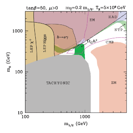
Figure 4: The same as in fig. 1 but for $T_{\rm R}=5\times 10^{9}\,\mbox{GeV}$ and $\tan\beta=10$ and $m_{\widetilde{G}}=m_{0}$ (left window) and $\tan\beta=10$ and $m_{\widetilde{G}}=0.2m_{1/2}$ (right window). Applying bounds from $D/H+Y_{p}$ derived with (25)–(26) as input rules out the cosmologically favored regions, as described in the text.

It is interesting that, in all the cases presented above for which $m_{\widetilde{G}}\propto m_{0}$, the (pale green) region of $\Omega^{\rm NTP}_{\widetilde{G}}h^{2}\sim 0.1$ is almost completely excluded by a combination of BBN and CMB constraints. In other words, for this case, a contribution to $\Omega_{\widetilde{G}}h^{2}$ from TP has to be substantial in order to escape the above constraints. On the other hand, this is not appear to be the case for $m_{\widetilde{G}}\propto m_{1/2}$.

6 Implications for Leptogenesis and SUSY Searches at the LHC

It is interesting that, in spite of tight and improving constraints from CMB and BBN, the possibility that in models of low energy SUSY with gravity–mediated SUSY breaking the gravitino may be the main component of the cold dark matter in the Universe remains open. Clearly this is the case when the reheating temperature $T_{\rm R}\mathrel{\hbox to0.0pt{\lower 4.0pt\hbox{\hskip 1.0pt$\sim$}\hss}\raise 1.0pt\hbox{$<$}}10^{9}\,\mbox{GeV}$ for which a contribution from thermal production can be neglected. Then the cosmologically favored regions due to NLSP decays (non–thermal production) alone shift to larger $m_{1/2}$, which is typically (albeit not always) somewhat less affected by the above constraints.

Perhaps even more interesting is the fact that the reheating temperatures as large as $5\times 10^{9}\,\mbox{GeV}$ seems to be allowed. This should be encouraging to those who favor thermal leptogenesis as a way of producing the baryon–antibaryon asymmetry in the Universe.

We stress that the above conclusions depend rather sensitively on the assumed input from BBN bounds. Given a number of outstanding discrepancies in determinations of the abundances of light elements, especially of ${{}^{6}}{\!Li}$ and ${{}^{3}}{\!He}$, in our analysis we have decided to apply rather conservative bounds derived using rather generous inputs, but also discussed the (severe) impact of sharpening them. In constraining electromagnetic fluxes we included bounds from $D/H+Y_{p}+{{}^{7}}{\!Li}$ derived with conservative inputs (22)–(24). We did not take into account bounds from ${{}^{6}}{\!Li}$ nor ${{}^{3}}{\!He}$ which otherwise would be most constraining. The constraints on hadronic fluxes that we have adopted are somewhat less conservative since they are based on less generous inputs (25)–(26) and on assuming $B_{had}=1$. Improvements in determining the above ranges is likely to provide a very stringent constraint on allowing high reheating temperatures $T_{\rm R}\sim 10^{9}\,\mbox{GeV}$, and perhaps even on the whole hypothesis of gravitino CDM in the CMSSM and similar models. Likewise, the (independent from BBN) bound from the CMB spectrum, if improved by at least one order of magnitude, is likely to prove highly constraining to the scenario. Certainly it would rule out the presented above cases of $T_{\rm R}=5\times 10^{9}\,\mbox{GeV}$. Finally, we have neglected other possible, although strongly model dependent, mechanisms of producing gravitinos, e.g. from inflaton decays, which could also contribute to $\Omega^{\rm NTP}_{\widetilde{G}}h^{2}$.

An experimental verification of the scenario will, for the most part, be rather challenging but not impossible. At the LHC one will have a good chance of exploring some interesting ranges of mass parameters. The most promising signature will be a detection of a massive, stable and electrically charged (stau) particle. In most cases, the cosmologically favored regions correspond to $m_{0}\mathrel{\hbox to0.0pt{\lower 4.0pt\hbox{\hskip 1.0pt$\sim$}\hss}\raise 1.0pt\hbox{$<$}}1\,\mbox{TeV}$ and large $m_{1/2}\mathrel{\hbox to0.0pt{\lower 4.0pt\hbox{\hskip 1.0pt$\sim$}\hss}\raise 1.0pt\hbox{$>$}}1\,\mbox{TeV}$, up to $2\,\mbox{TeV}$ at small $\tan\beta$, and $4\,\mbox{TeV}$ at large $\tan\beta$. A significant fraction of this region should be explored in the stau mode since $m_{{\tilde{\tau}}_{1}}^{2}\simeq m_{0}^{2}+0.15m_{1/2}^{2}$ and stable stau mass will probably be probed up to $\sim 1\,\mbox{TeV}$. Gluino search may be less promising since $m_{1/2}\mathrel{\hbox to0.0pt{\lower 4.0pt\hbox{\hskip 1.0pt$\sim$}\hss}\raise 1.0pt\hbox{$>$}}1\,\mbox{TeV}$ implies $m_{\tilde{g}}\mathrel{\hbox to0.0pt{\lower 4.0pt\hbox{\hskip 1.0pt$\sim$}\hss}\raise 1.0pt\hbox{$>$}}2.7\,\mbox{TeV}$, which will be just outside of the reach of the LHC. However, some interesting cases may still be explored. One is that of fairly small $\tan\beta$ and $m_{\widetilde{G}}\propto m_{0}$, as in the left windows of figs. 2 and 4. The other is that of large $\tan\beta$ and large $T_{\rm R}$, as in the right window of fig. 4. On the other hand, since in the cosmologically favored regions $m_{0}\ll m_{1/2}$ squarks (and sleptons) will be fairly light and lighter than the gluino. More work will be needed to more fully assess to what extend the cosmologically favored regions will be explored at the LHC. Finally, the staus will eventually decay. The proposal of [62] of measuring their delayed decays is in this context worth pursuing as it would give a unique opportunity of experimentally exploring the hypothesis of gravitino cold dark matter and of probing the Planck scale at the LHC.

- [1] A.D. Dolgov and Ya.B. Zel´dovich, Rev. Mod. Phys. 53 (1981) 1.
- [2] H. Pagels and J.R. Primack, Phys. Rev. Lett. 48 (1982) 223.
- [3] S. Weinberg, Phys. Rev. Lett. 48 (1982) 1303.
- [4] M.Y. Khlopov and A. Linde, Phys. Lett. B 138 (1984) 265.
- [5] J.R. Ellis, J.E. Kim and D.V. Nanopoulos, Phys. Lett. B 145 (1984) 181.
- [6] J.R. Ellis, D.V. Nanopoulos and S. Sarkar, Nucl. Phys. B 259 (1985) 175.
- [7] D.V. Nanopoulos, K.A. Olive and M. Srednicki, Phys. Lett. B 127 (1983) 30.
- [8] R. Juszkiewicz, J. Silk and A. Stebbins, Phys. Lett. B 158 (1985) 463.
- [9] M. Kawasaki and T. Moroi, Prog. Theor. Phys. 93 (1995) 879 [arXiv:hep-ph/9403364].
- [10] R.H. Cyburt, J. Ellis, B.D. Fields and K.A. Olive, Phys. Rev. D 67 (2003) 103521 [arXiv:astro-ph/0211258].
- [11] M. Kawasaki, K. Kohri and T. Moroi, arXiv:astro-ph/0402490 and arXiv:astro-ph/0408426.
- [12] T. Moroi, H. Murayama and M. Yamaguchi, Phys. Lett. B 303 (1993) 289.
- [13] R. D. Peccei and H. R. Quinn, Phys. Rev. Lett. 38 (1977) 1440 and Phys. Rev. D 16 (1977) 1791.
- [14] J. E. Kim, A. Masiero and D. V. Nanopoulos, Phys. Lett. B 139 (1984) 346.
- [15] S. A. Bonometto, F. Gabbiani and A. Masiero, Phys. Lett. B 222 (1989) 433 and Phys. Rev. D 49 (1994) 3918 [arXiv:hep-ph/9305237].
- [16] K. Rajagopal, M. S. Turner and F. Wilczek, Nucl. Phys. B 358 (1991) 447.
- [17] L. Covi, H. B. Kim, J. E. Kim and L. Roszkowski, J. High Energy Phys. 05 (2001) 033 [arXiv:hep-ph/0101009].
- [18] T. Asaka and T. Yanagida, Phys. Lett. B 494 (2000) 297 [arXiv:hep-ph/0006211].
- [19] L. Covi, J. E. Kim and L. Roszkowski, Phys. Rev. Lett. 82 (1999) 4180 [arXiv:hep-ph/9905212].
- [20] L. Covi, L. Roszkowski and M. Small, J. High Energy Phys. 07 (2002) 023 [arXiv:hep-ph/0206119].
- [21] A. Brandenburg and F.D. Steffen, J. Cosmol. Astrop. Phys. 08 (008) 2004 [arXiv:hep-ph/0405158].
- [22] M. Bolz, W. Buchmüller and Plümacher, Phys. Lett. B 443 (1998) 209 [arXiv:hep-ph/9809381].
- [23] M. Bolz, A. Brandenburg and W. Buchmüller, Nucl. Phys. B 606 (2001) 518 [arXiv:hep-ph/0012052].
- [24] M. Fukugita and T. Yanagida, Phys. Lett. B 174 (1986) 45.
- [25] L. Covi, E. Roulet and F. Vissani, Phys. Rev. D 384 (1996) 169 [arXiv:hep-ph/9605319].
- [26] G.F. Giudice, A. Notari, M. Raidal, A. Riotto and A. Strumia, Nucl. Phys. B 685 (2004) 89 [arXiv:hep-ph/031012].
- [27] J.L. Feng, A. Rajaraman and F. Takayama, Phys. Rev. Lett. 91 (2003) 011302 [arXiv:hep-ph/0302215].
- [28] J.L. Feng, A. Rajaraman and F. Takayama, Phys. Rev. D 68 (2003) 063504 [arXiv:hep-ph/0306024].
- [29] J.L. Feng, S. Su and F. Takayama, arXiv:hep-ph/0404198.
- [30] J.L. Feng, S. Su and F. Takayama, arXiv:hep-ph/0404231.
- [31] J. Ellis, K.A. Olive, Y. Santoso and V. Spanos, Phys. Lett. B 588 (2004) 7 [arXiv:hep-ph/0312262].
- [32] G. L. Kane, C. Kolda, L. Roszkowski, and J. D. Wells, Phys. Rev. D 49 (1994) 6173 [arXiv:hep-ph/9312272].
- [33] T. Asaka, K. Hamaguchi and K. Suzuki, Phys. Lett. B 490 (2000) 136 [arXiv:hep-ph/0005136].
- [34] T. Gherghetta, G.F. Giudice and A. Riotto, Phys. Lett. B 446 (1999) 28 [arXiv:hep-ph/9808401].
- [35] G.F. Giudice, A. Riotto and I. Tkachev, J. High Energy Phys. 9911 (1999) 036 [arXiv:hep-ph/9911302] and J. High Energy Phys. 9908 (1999) 009 [arXiv:hep-ph/9907510].
- [36] R. Kallosh, L. Kofman, A. Linde and A. Van Proeyen, Phys. Rev. D 61 (2000) 103503 [arXiv:hep-th/9907124].
- [37] H.P. Nilles, M. Peloso and L. Sorbo, Phys. Rev. Lett. 87 (2001) 051302 [arXiv:hep-ph/0102264].
- [38] For a recent analysis, see K. Kohri, M. Yamaguchi and J. Yokoyama, arXiv:hep-ph/0403043.
- [39] D. Hooper and L.-T. Wang, arXiv:hep-ph/0402220.
- [40] E.W. Kolb and M.S. Turner, The Early Universe, Addison-Wesley (1990).
- [41] T. Moroi, PhD thesis, arXiv:hep-ph/9503210.
- [42] T. Nihei, L. Roszkowski, R. Ruiz de Austri, J. High Energy Phys. 05 (2001) 063 [arXiv:hep-ph/0102308].
- [43] T. Nihei, L. Roszkowski, R. Ruiz de Austri, J. High Energy Phys. 03 (2002) 031 [arXiv:hep-ph/0202009].
- [44] J. Edjö and P. Gondolo, Phys. Rev. D 56 (1997) 1879 [arXiv:hep-ph/9704361].
- [45] T. Nihei, L. Roszkowski, R. Ruiz de Austri, J. High Energy Phys. 07 (2002) 024 [arXiv:hep-ph/0206266].
- [46] L. Roszkowski, R. Ruiz de Austri and T. Nihei, J. High Energy Phys. 08 (2001) 024 [arXiv:hep-ph/0106334].
- [47] L. Covi, L. Roszkowski, R. Ruiz de Austri and M. Small, J. High Energy Phys. 0406 (2004) 003 [arXiv:hep-ph/0402240].
- [48] M.H. Reno and D. Seckel, Phys. Rev. D 37 (1988) 3441.
- [49] S. Dimopoulos, R. Esmailzadeh, L.J. Hall and G.D. Starkman, Astrophys. J. 330 (1988) 545 and Nucl. Phys. B 311 (1989) 699.
- [50] K. Jedamzik, Phys. Rev. D 70 (2004) 063524 [arXiv:astro-ph/0402344].
- [51] K. Jedamzik, Phys. Rev. Lett. 84 (2000) 3248 [arXiv:astro-ph/9909445].
- [52] G. Sigl, K. Jedamzik, D.N. Schramm, V.S. Berezinsky, Phys. Rev. D 52 (1995) 6682 [arXiv:astro-ph/9503094].
- [53] D. N. Spergel, et al., Astrophys. J. 148 (2003) 175 [arXiv:astro-ph/0302209].
- [54] C. L. Bennett, et al., Astrophys. J. 148 (2003) 1 [arXiv:astro-ph/0302207].
- [55] D. J. Fixsen, et al., Astrophys. J. 473 (1996) 576 [astro-ph/9605054]; K. Hagiwara, et al., [Particle Data Group], Phys. Rev. D 66 (2002) 010001.
- [56] W. Hu and J. Silk, Phys. Rev. Lett. 70 (1993) 2661 and Phys. Rev. D 48 (1993) 485.
- [57] K. Hagiwara, et al., Phys. Rev. D 66 (2002) 010001.
- [58] LEPSUSYWG, ALEPH, DELPHI, L3 and OPAL experiments, note LEPSUSYWG/01-03.1 (http://lepsusy.web.cern.ch/lepsusy/Welcome.html).
- [59] K. Okumura and L. Roszkowski, Phys. Rev. Lett. 92 (2004) 161801 [arXiv:hep-ph/0208101] and J. High Energy Phys. 0310 (2003) 024 [arXiv:hep-ph/0308102].
- [60] A. Djouadi, J.-L. Kneur and G. Moultaka. The package SUSPECT is available at http://www.lpm.univ-montp2.fr:7082/~kneur/suspect.html.
- [61] See, e.g., L. Cerrito, arXiv:hep-ex/0405046.
- [62] W. Buchmüller, K. Hamaguchi, M. Ratz and T. Yanagida, Phys. Lett. B 588 (2004) 90 [arXiv:hep-ph/0402179].