The $K$–matrix approach to the $\Delta-$ resonance mass–splitting
and isospin–violation in low–energy $\pi N$ scattering

Аннотация

Experimental data on $\pi N$ scattering in the elastic energy region $T_{\pi}\leq$ 250 MeV are analyzed within the multichannel $K$–matrix approach with effective Lagrangians. Isospin–invariance is not assumed in this analysis and the physical values for masses of the involved particles are used. The corrections due to $\pi^{+}-\pi^{0}$ and $p-n$ mass differences are calculated and found to be in a reasonable agreement with the NORDITA results. The results of our analysis describe the experimental observables very well. New values for mass and width of the $\Delta^{0}$ and $\Delta^{++}$ resonances were obtained from the data. The isospin–symmetric version yields phase–shifts values similar to the new solution, FA02, for the $\pi N$ elastic scattering amplitude by the GW group based on the latest experimental data. While our analysis leads to a considerably smaller ($\leq$1%) isospin–violation in the energy interval T${}_{\pi}\sim$30–70 MeV as compared to 7% in works by Gibbs et al. and Matsinos, it confirms calculations based on Chiral Perturbation Theory.

I Introduction

Low–energy pion–nucleon scattering is one of the fundamental processes that test the low–energy QCD regime $-$ the pion is a Goldstone boson in the chiral limit, where the $\pi N$ interaction goes to zero at zero energy. This behavior is modified by explicit chiral-symmetry breaking by the small masses of the up and down quarks, $M_{u}\approx$ 5 MeV and $M_{d}\approx$ 9 MeV leut . Since quark masses are not equal, the QCD Lagrangian contains the isospin–violating term $\propto(M_{u}-M_{d})$. Calculations using Chiral Lagrangians weinb and Chiral Perturbation Theory meiss predict isospin–violation effects for the low–energy $\pi^{\pm}N$ elastic scattering and charge–exchange (CEX) reactions $\sim 1$%. However, for the case of the much smaller $\pi^{0}N$ elastic scattering, isospin–breaking is $\approx$25%. Therefore, to observe the isospin–violation effects, particular experimental conditions are needed, where these effects are enhanced due to kinematics or other reasons. One such experiment is found in the $\Delta(1232)$ resonance mass–splitting measurement. In this case, close to the $\Delta(1232)$ resonance position, the phase–shifts vary rapidly with the energy. Therefore, the small ($\leq$1%) difference among the masses of the different isospin–states of the $\Delta(1232)$ resonance as measured in different scattering channels leads to significant differences for the corresponding phase–shifts. The usual procedure for extracting the $\Delta(1232)$ resonance mass–splitting from the data is in a phase–shift analysis pedroni ; koch ; abav ; bugg ; fa02 , where the $P_{33}$ partial–wave amplitude from $\pi^{+}p$, $\pi^{-}p$, and charge exchange data are considered as independent quantities. These phase–shifts were then fitted by a Breit–Wigner (BW) formula to determine the corresponding resonance parameters. The disadvantage of this procedure is in using isospin–symmetric quantities in a situation where isospin is not conserved.

Two phenomenological analyses of $\pi N$ scattering data at low–energies T${}_{\pi}\sim$30–70 MeV gibbs ; mat reported about 7% isospin–violation in the ‘‘triangle relation":

$$f(\pi^{-}p\to\pi^{0}n)=\frac{f(\pi^{+}p)-f(\pi^{-}p)}{\sqrt{2}}.$$ (1)

This is significantly larger than is predicted in  meiss and very important for the determination of the $\Delta(1232)$ resonance mass–splitting, meaning that an isospin–violation occurs in the background as well. But this conclusion is based on the rather old and incomplete experimental data, especially on the charge–exchange reaction. Note, that the analysis gibbs used preliminary low–energy $\pi^{\pm}$ elastic scattering data psi , while in the final form jo , these data were increased by 10% in the absolute values and the pion energies were decreased (shifted) by 1 MeV or more. In recent years, progress has been made in this input – new high–quality experimental data have been published (see isaid for the up–to–date database). In particular, detailed experimental data on $\pi^{-}p\to\pi^{0}n$ reaction at very low–energy are reported in isenh . Several years ago, a $K$–matrix approach with effective Lagrangians was developed goud ; gri ; feu and found to be in good agreement with all $\pi N$ observables in the entire elastic energy region. In the present paper, we modify this approach to estimate the isospin–violating effects in the new low–energy, $T_{\pi}\leq 250$ MeV, $\pi N$ scattering database.

II Tree–Level Model for the $K$–matrix

The detailed description of the isospin–invariant version of the multichannel $K$–matrix approach used in this analysis can be found in goud ; gri . It is assumed that the $K$–matrix, being a solution of the Bethe–Salpeter equation, can be considered as a sum of the tree–level Feynman diagrams with the effective Lagrangians in the vertices. Real part of the loops leads to renormalization of the mass and couplings. We assume that energy dependence of the vertex functions in the restricted energy interval can be accounted for by expansion of these function on power of invariants. This leads to Lagrangians, which contain the derivatives of the fields. In gri , it was demonstrated that such approach work very well in isospin–symmetric case up to $T_{\pi}\sim$ 900 MeV. Here we restrict ourselves the $\Delta$–resonance energy region $T_{\pi}<$ 250 MeV. Because we want to look for possible isospin–violation, we describe $\pi N$ scattering using the same diagrams as in goud ; gri , only in the charged–channels formalism. We confine ourselves to $\pi^{\pm}p$ and $\pi^{0}n$ channels to be able to compare the calculations with the experimental data. At the hadronic level, the $\pi^{+}p$ scattering is a single–channel problem and the corresponding Feynman diagrams are shown in Fig. 1. The $\pi^{-}p$ scattering includes two–channels, one due to the nonzero $\pi^{-}p\to\pi^{0}n$ reaction. Feynman diagrams for this amplitude are presented in Fig. 2. The same Lagrangians as in goud ; gri were used in the calculations, but the coupling constants are considered, in general, to be different for the different channels. The masses of the incoming and outgoing particles were taken as masses of the physical particles from PDG pdg . The masses of the intermediate particles can be different for different channels as well and for the $\Delta(1232)$ resonance we determine masses of $\Delta^{++}$ and $\Delta^{0}$ from the fit of experimental data. The interaction Lagrangian, corresponding to the $\pi NN$ vertex, has the structure

$$L_{\pi NN}=-\frac{g_{\pi_{i},N_{k},N_{l}}}{1+x_{i,k,l}}\overline{\Psi}_{k}\gamma_{5}\left(ix_{i,k,l}\pi_{i}+\frac{1}{m_{k}+m_{l}}\gamma_{\mu}\partial^{\mu}{\pi_{i}}\right)\Psi_{l}+{\rm h.c.},$$ (2)

where i,k,l indexes mean pion, left, and right nucleon charged states. The vertex is assumed to have both pseudoscalor and pseudovector parts with the mixing parameter $x_{i,k,l}$.

The interaction Lagrangian, corresponding to the $\pi N\Delta$ vertex, reads as

$$L_{\pi N\Delta}=\frac{g_{\pi_{i},\Delta_{k},N_{l}}}{M_{\Delta_{k}}+m}\overline{\Psi}_{k}^{\mu}\theta_{\mu\nu}T_{kl}\Psi_{N_{l}}\partial^{\nu}\pi_{i}+{\rm h.c.},$$ (3)

$$\theta_{\mu\nu}=g_{\mu\nu}-\left(Z_{\Delta_{k}}+\frac{1}{2}\right)\gamma_{\mu}\gamma_{\nu}.$$ (4)

Here, $T_{kl}$ denotes the transition operator between nucleon and $\Delta$–isobar.We treat the $\Delta$ -isobar graphs in the most general manner; thus, constants $Z_{\Delta_{k}}$ and $g_{\pi_{i},\Delta_{k},N_{l}}$ will be determined from our fit to the experimental data

The interaction Lagrangian for the $\rho\pi\pi$ vertex is put in the form

$$L_{\rho\pi\pi}=-g_{\rho_{i}\pi_{k}\pi_{l}}\rho^{\mu}_{i}\left(\partial^{\mu}\pi_{k}\pi_{l}-\partial^{\mu}\pi_{l}\pi_{k}\right)$$ (5)

and for the $\rho$NN vertex

$$L_{\rho NN}=-g_{\rho_{i}N_{k}N_{l}}\overline{\Psi}_{k}\frac{1}{2}\left(\gamma_{\mu}\rho^{\mu}_{i}+\frac{2\kappa}{m_{k}+m_{l}}\sigma_{\mu\nu}\partial^{\mu}\rho^{\nu}_{i}\right)\Psi_{l}+{\rm h.c.}$$ (6)

where $\kappa$ is the tensor and vector coupling constant ratio. For $\sigma\pi\pi$ and $\sigma NN$ interaction, the following form of the Lagrangians are used:

$$L_{\sigma\pi\pi}=-g_{\sigma\pi_{i}\pi_{i}}\pi_{i}\pi_{i}\sigma,$$ (7)

$$L_{\sigma NN}=-g_{\sigma N_{i}N_{i}}\overline{\Psi}_{i}\Psi_{i}\sigma.$$ (8)

Thus, for isospin–symmetric case, we have seven free parameters: $G_{\rho}^{V}=\frac{g_{\rho NN}g_{\rho\pi\pi}}{m_{\rho}^{2}}$, $G_{\sigma\pi}=\frac{g_{\sigma NN}g_{\sigma\pi\pi}}{m_{\sigma}^{2}}$, $\kappa$, $g^{2}_{\pi NN}/4\pi$, $x_{\pi N}$, $g_{\pi N\Delta}$, and $Z_{\Delta}$. But futher we assume different coupling constants for different charged channels, therefore, the number of free parameters will increase.

The scattering amplitudes can be calculated as:

$$f(\pi^{+}p\to\pi^{+}p)=\frac{\tilde{K}_{\pi^{+}p}}{1-i\tilde{K}_{\pi^{+}p}},$$ (9)

$$f(\pi^{-}p\to\pi^{-}p)=\frac{\tilde{K}_{\pi^{-}p}-i(\tilde{K}_{\pi^{-}p}\tilde{K}_{\pi^{0}n}-\tilde{K}_{\pi^{-}p\to\pi^{0}n}^{2})}{\tilde{K}_{\pi^{-}p}\tilde{K}_{\pi^{0}n}-\tilde{K}_{\pi^{-}p\to\pi^{0}n}^{2}-i(\tilde{K}_{\pi^{-}p}+\tilde{K}_{\pi^{0}n})},$$ (10)

$$f(\pi^{-}p\to\pi^{0}n)=\frac{\tilde{K}_{\pi^{-}p\to\pi^{0}n}}{\tilde{K}_{\pi^{-}p}\tilde{K}_{\pi^{0}n}-\tilde{K}_{\pi^{-}p\to\pi^{0}n}^{2}-i(\tilde{K}_{\pi^{-}p}+\tilde{K}_{\pi^{0}n})},$$ (11)

$$f(\pi^{0}n\to\pi^{0}n)=\frac{\tilde{K}_{\pi^{0}n}-i(\tilde{K}_{\pi^{-}p}\tilde{K}_{\pi^{0}n}-\tilde{K}_{\pi^{-}p\to\pi^{0}n}^{2})}{\tilde{K}_{\pi^{-}p}\tilde{K}_{\pi^{0}n}-\tilde{K}_{\pi^{-}p\to\pi^{0}n}^{2}-i(\tilde{K}_{\pi^{-}p}+\tilde{K}_{\pi^{0}n})},$$ (12)

where, for example, $\tilde{K}_{\pi^{0}n}$ is the $K$–matrix element for $\pi^{0}n\to\pi^{0}n$ channel multiplied by c.m. momentum of the $\pi^{0}n$ system to obtain the dimensionless scattering amplitudes in Eqs. (9–12).

III Electromagnetic corrections

In the analysis of the pion–nucleon experimental data, the  $SU(2)$ isospin–symmetry is usually assumed. This implies that the masses of the isospin–multiplet must be equal. However, the physical masses of the particles are different. There are two sources for this mass–splitting: the electromagnetic self–energy and the QCD quark mass difference. The latter leads to isospin–violating effects in the strong interaction. Usually the influence of the mass difference on the pion–nucleon scattering amplitude is calculated together with the true electromagnetic corrections. The most popular way to do this is the method of the effective potential gashi and dispersion relations trom .

There are several reasons for using $K$–matrix approach to calculate the mass difference corrections (MDC) to the pion–nucleon amplitude:

• Only the mass–splitting of the external particles (pions and nucleons) have been taken into account up to now. In the $K$–matrix approach, corrections due to mass difference of all particles in the intermediate state can be calculated explicitly.

• MDC contributions dominate the structure of the total $P$–waves corrections trom . Therefore, it is important to estimate them by different methods to obtain reliable results.

Let us start with $\pi^{-}p$ elastic scattering. In general, the $S$–matrix for the charged channels has the form:

$$S_{c}=\left(\begin{array}[]{cccc}S_{\pi^{-}p}&;&S_{\pi^{-}p\to\pi^{0}n}\\ S_{\pi^{0}n\to\pi^{-}p}&;&S_{\pi^{0}n}\end{array}\right).$$ (15)

Time–reversal invariance is assumed, thus, $S_{\pi^{-}p\to\pi^{0}n}$ = $S_{\pi^{0}n\to\pi^{-}p}$. If  $SU(2)$ isospin–symmetry is valid, then the unitarity matrix

$$U_{t}=\frac{1}{\sqrt{3}}\left(\begin{array}[]{cccc}-\sqrt{2}&;&1\\ 1&;&\sqrt{2}\end{array}\right)$$ (18)

can be used for the transformation of the $S_{c}$ to the isospin–basis

$$S_{I}=U_{t}^{+}S_{c}U_{t}.$$ (19)

In this case, the isospin–channels are eigenchannels, therefore, $S_{I}$ must be diagonal:

$$S_{I}^{H}=\left(\begin{array}[]{cccc}\eta_{H1}e^{2i\delta_{H1}}&;&0\\ 0&;&\eta_{H3}e^{2i\delta_{H3}}\end{array}\right).$$ (22)

Here the index H means that quantities are calculated for eigenchannels. If isospin–symmetry is slightly violated, then the transformation (19) leads to nondiagonal matrix elements. To be able to compare the results with trom , we write the $S$–matrix for this case in the following form:

$$S_{I}=\left(\begin{array}[]{cccc}\eta_{1}e^{2i\delta_{1}}&;&\frac{2}{3}\sqrt{2}(\eta_{13}+i\Delta_{13})e^{i(\delta_{1}+\delta_{3})}\\ \frac{2}{3}\sqrt{2}(\eta_{13}+i\Delta_{13})e^{i(\delta_{1}+\delta_{3})}&;&\eta_{3}e^{2i\delta_{3}}\end{array}\right).$$ (25)

Then, the corrections to the isospin–symmetric matrix $S_{I}^{H}$, apart from $\Delta_{13}$ and $\eta_{13}$ are defined as:

$$\delta_{1}=\delta_{H1}-\frac{2}{3}\Delta_{1}\leavevmode\nobreak\ ;\leavevmode\nobreak\ \bar{\eta}_{1}=\eta_{H1}-\eta_{1};$$

$$\delta_{3}=\delta_{H3}-\frac{1}{3}\Delta_{3}\leavevmode\nobreak\ ;\leavevmode\nobreak\ \bar{\eta}_{3}=\eta_{H3}-\eta_{3}.$$ (26)

There are different contributions to these corrections: due to electromagnetic interactions, mass–splitting, $n\gamma$ channel, etc. Here, we are only interested in the mass–splitting contribution. In order to calculate it, the isospin–symmetric reference masses have to be fixed. The conventional choices are $m=M_{p}$ for the nucleon, $M_{\pi}=M_{\pi^{\pm}}$ for the charged pions, and $M_{\Delta}$ = 1232 MeV is added for the $\Delta(1232)$ resonance. The procedure of the calculations is as follows. First we use the $K$–matrix with the physical masses to calculate the $S$–matrix for the charged channels $S_{c}$. Then, we transform $S_{c}$ to isospin–basis by matrix (18) and obtain the corrections $\Delta_{13},\eta_{13}$ and the quantities $\eta_{1},\delta_{1},\eta_{3}$, and $\delta_{3}$. After that, we repeat the calculations with the isospin–symmetric reference masses and obtain the values $\eta_{H1},\delta_{H1},\eta_{H3}$, and $\delta_{H3}$. Finally, the corrections $\bar{\eta}_{1},\Delta_{1},\bar{\eta}_{3}$, and $\Delta_{3}$ are found.

For the $\pi^{+}p$ scattering, we use the one–channel form for the nuclear $S_{\pi^{+}p}$ and the hadronic $S_{H}$ matrices (see trom for the definition of the terms):

$$S_{\pi^{+}p}=\eta_{3}^{+}e^{2i\delta_{3}^{+}}\leavevmode\nobreak\ ;\leavevmode\nobreak\ S_{H}=\eta_{H3}^{+}e^{2i\delta_{H3}^{+}},$$ (27)

and the similar formulae for the corrections:

$$\delta_{3}^{+}=\delta_{H3}^{+}-\frac{1}{3}\Delta_{3}^{+}\leavevmode\nobreak\ ;\leavevmode\nobreak\ \bar{\eta}_{3}^{+}=\eta_{H3}^{+}-\eta_{3}^{+}.$$ (28)

We find that contribution of the mass–splitting effect on the inelasticity corrections $\bar{\eta}_{1},\bar{\eta}_{3}$, and $\bar{\eta}_{3}^{+}$ is very small (less than $10^{-4}$) and can be neglected.

In Fig. 3, the most important $\Delta_{3}$ mass difference correction for total angular momentum J = 3/2 is presented (solid line) together with that from  trom (dashed line). The $\Delta(1232)$ resonance mass–splitting is not taken into account in this figure, as it was in trom . But it was found that $\Delta(1232)$ resonance mass–splitting leads to very large effect for the $\Delta_{3}$ correction (this is the correction to $P_{33}$ phase–shifts). The origin of that comes from the rapid variation of phase shift near the resonance position. Therefore, the small change in the $\Delta(1232)$ mass corresponds to a large phase shift difference. This $\Delta(1232)$ resonance mass–splitting effect is not contained in the NORDITA  trom corrections. Therefore, if one wants to extract hadronic isospin–symmetric amplitudes, based on the NORDITA procedure, one has to include the $\Delta(1232)$ mass–splitting effect. If $\Delta(1232)$ mass–splitting effect is not included, then $P_{33}$ phase–shifts determined from $\pi^{+}p$ and $\pi^{-}p$ will be different trom ; abav . These results for other partial–waves are small and of the same order as true electromagnetic ones.

IV Database and fitting procedure

For a definite set of the coupling constants and particle masses, the hadronic part of the amplitude was calculated according to graphs in Figs. 1 and 2. The electromagnetic interaction was added in order to compare with experimental data. We use the observed masses of the particles, therefore, the electromagnetic parts of NORDITA corrections were included only using isospin–invariance relations. It was found, however, that the latter do not affect the values of the extracted parameters within the uncertainties and can be neglected. In order to determine the parameters of the model, the standard MINUIT CERN library program minuit was used. The experimental data used here are those $\pi N$ data which can be found in the SAID database isaid . In the present work, we confine ourselves to partial–waves with spin 1/2 and 3/2. Only for these can the Lagrangians be written in ‘‘conventional"way (see discussion on Lagrangian for spin 3/2 particles in nieu ). The inelastic channels are not included in the present version of the model; therefore, only the data below T_π = 250 MeV are used in the fit. In this energy region, there are no open inelastic channels and the $S$ and $P$ partial–waves give the dominant contribution to the observables. The small contributions of the higher partial–waves were taken from the partial–wave analyses. The different partial–wave analyses (KH80 koch , KA84 ka84 , KA85 ka85 , SM95 sm95 , and FA02 fa02 ) lead to similar results, and only the latest FA02 solution was used in all further calculations. As a rule, the parameter values obtained by fit have very small uncertainties. Therefore, the main source of these uncertainties comes from the database. To estimate it, we perform the fit in two steps. First, we take all data in the first fit. Then remove the data points which give more than 4 in $\chi^{2}$ units (mainly from jo ; br )and perform a second fit. The number of such points is about 2%. We take the difference in the parameter values in these two fits as the uncertainties of the parameter. It was found that rejection of more data leads to parameter values within the uncertainties determined above. Typically, a $\chi^{2}\sim 1.5$ was obtained. The largest contribution to $\chi^{2}$ comes from $\pi^{-}p$ elastic scattering data.

V Results and discussion

As a first step, and in order to reduce the number of the free parameters, we assume the coupling constant entering the interaction Lagrangians to be isospin–invariant. Thus, we have nine free parameters – seven for coupling constants goud and two for $M_{\Delta^{++}}$ and $M_{\Delta^{0}}$. The results for the coupling constants were found to be similar to those from goud and are presented in the Table 1. The value of $g_{\pi NN}^{2}/4\pi$ = 13.80 agrees very well with the recent result $g^{2}_{\pi NN}/4\pi$ = 13.75 $\pm$ 0.10 from FA02 solution fa02 .

In order to determine the resonance parameters, we should assume some procedure to separate the resonance and background contributions to the amplitude. In general, such a procedure is somewhat arbitrary woolc . The most popular way is to write the BW formula for the scattering amplitude near the resonance position. For the one–channel case ($\pi^{+}p$ scattering), this corresponds to defining the mass of the resonance as the pole position of the corresponding $K$–matrix. Indeed, close to the pole the $K$–matrix has a form:

$$K(w)=\frac{\alpha^{2}}{w-M}+\beta(w),$$ (29)

where $\alpha$ and $\beta(w)$ are a smooth functions of the energy. Then in this region the scattering amplitude obtains the BW form:

$$F(w)=\frac{K}{1-iqK}=\frac{\alpha^{2}+\beta(w)(w-M)}{w-M+iq[\alpha^{2}+\beta(w)(w-M)]}\approx\frac{\alpha^{2}}{w-M+iq\alpha^{2}}.$$ (30)

Therefore, the width of the resonance is read as

$$\Gamma_{\Delta^{++}}=2\lim_{w\to M_{\Delta^{++}}}(w-M_{\Delta^{++}})\leavevmode\nobreak\ q_{\pi^{+}}K_{\pi^{+}p}.$$ (31)

For the two–channel case ($\pi^{-}$p scattering), the form of amplitudes (10–12) is more complicated. But the situation can be improved using the eigenchannel representation. This means that we define the new channel basis to transform the $K$–matrix into the diagonal form K^ech = $U^{+}KU$, where $U$ is the unitary transformation matrix. At the same time, the matrix of amplitudes also becomes diagonal. Only one channel contains the resonance in this representation (see Appendix in  gri for details) with the same pole position. For this channel, the amplitude has a BW form as in the one–channel case. In order to calculate the width of the resonance, trace conservation under unitarity transformations $tr(K^{ech})=tr(K)$ is used. Therefore:

$$\Gamma_{\Delta^{0}} = 2\lim_{w\to M_{\Delta^{0}}}(w-M_{\Delta^{0}})tr(K^{ech})=2\lim_{w\to M_{\Delta^{0}}}(w-M_{\Delta^{0}})tr(K)$$ (32)

$$= 2\lim_{w\to M_{\Delta^{0}}}(w-M_{\Delta^{0}})\left(q_{\pi^{-}}K_{\pi^{-}p}+q_{\pi^{0}}K_{\pi^{0}n}\right).$$

In order to clarify the procedure, let us consider as an example the $\pi^{-}p$ scattering, when the isospin is conserved. The charged channels are $\pi^{-}p\to\pi^{-}p$ and $\pi^{-}p\to\pi^{0}n$. So, the scattering amplitude is a $2\times 2$ matrix. After transforming this matrix from the charged–channel basis to isotopic one, we get a $2\times 2$ diagonal matrix. Now only one channel with isospin 3/2 contains the resonance ($\Delta(1232)$).

Our fitting procedure leads to reasonable values for masses and widths of the $\Delta(1232)$ isobar; these are presented in the Table 2 together with PDG data. It should be noted that all values from PDG were not obtained directly from the data as in the present work, but by using the results of the phase shift analyses for individual charged channels. Then, the resulting amplitudes (or remaining part of data as in  fa02 ) are fitted by some simple BW formula. The graphs in Figs. 1 and 2 with $\Delta(1232)$ resonance in the intermediate state give contributions not to $P_{33}$ partial–wave only, but to all other waves too. As a result, in the resonance region, we found the 1% isospin–violation in $S_{31}$ and somewhat smaller in $P_{31}$ partial–waves due to difference in the $\Delta(1232)$ masses. This was not accounted for in above procedure, but it is important in determining the $\Delta(1232)$ width because of the rather wide energy interval used in the fit. This can account for the large spread of $\Gamma_{\Delta^{0}}-\Gamma_{\Delta^{++}}$ values in the Table 2. In our approach, the fit to different data combinations ($(\pi^{+},\pi^{-}),\leavevmode\nobreak\ (\pi^{+},CEX)$, and $(\pi^{-},CEX)$) gives the same values for all parameters with slightly larger uncertainties.

We obtain equal coupling constants in all charged channels (see below), therefore, the difference in the $\Delta(1232)$ widths has two sources: the difference in phase space due to different $\Delta(1232)$ masses (this gives 3.7 MeV) and different masses of final particles in the $\Delta^{0}\to\pi^{0}n$ and $\Delta^{++}\to\pi^{+}p$ decays (this gives 0.9 MeV). We obtain $\Gamma_{\Delta^{0}\to\pi^{0}n}/\Gamma_{\Delta^{0}\to\pi^{-}p}$ = 2.024 instead of 2.0 for the isospin–invariant case. There is also an additional $\sim$ 1 MeV contribution to the $\Delta^{0}$ width from the $\Delta^{0}\to\gamma n$ decay, which is not included in present version of the model. In Refs. abav ; bugg , the quantities $\delta^{++}_{33}(w),\leavevmode\nobreak\ \delta^{0}_{33}(w)$, and $\eta^{0}_{33}(w)$ via

$$f^{3/2}_{\pi^{+}p}(w)=\frac{e^{2i\delta^{++}_{33}(w)}-1}{2iq_{\pi^{+}}},$$ (33)

$$f^{3/2}_{\pi^{-}p}(w)+\sqrt{2}f^{3/2}_{\pi^{-}p\to\pi^{0}n}(w)=\frac{\eta^{0}_{33}(w)e^{2i\delta^{0}_{33}(w)}-1}{2iq_{\pi^{-}}}$$ (34)

were determined from the experimental data. In Figs. 4 and 5, we compare calculated values for $\delta^{++}_{33}(w)-\delta^{0}_{33}(w)$ and  $\eta^{0}_{33}(w)$ with the results of Refs. abav ; bugg . As it is seen from the figures, the agreement is very good up to $W\approx$1.3 GeV. As was found in abav at higher energies, the difference $\delta^{++}_{33}(w)-\delta^{0}_{33}(w)$ changes sign. Such behavior cannot be explained within our approach. However, just at these energies an inelastic two–pion production process opens; the difference in the pion masses is a probable source of this phenomena. In Fig. 6, the phase–shifts for the isospin–symmetric case (masses of all particles were set to conventional values) are shown together with the results of phase–shift analyses KH80 and FA02 – our results are not in conflict with the known phase shift analyses. In fett a large discrepancy between calculations based on Chiral Perturbation Theory and results of phase shift analysis in $S$–waves was found for $P_{\pi}<$ 100 MeV/c. From Fig. 6 we see that there is no such a discrepancy in our approach.

As a next step, we tried to allow some coupling constants to be different for different charged channel. No statistically proved differences in the $g_{\pi^{+}NN},g_{\pi^{-}NN}$, and $g_{\pi^{0}NN}$ or other coupling constants were found. It is interesting to note that all fits give nearly equal values of $g_{\pi N\Delta}$ for all charged channels with very small uncertaintie, less then 0.2%. In Fig. 4, the dashed line shows the results for $\delta^{++}_{33}(w)-\delta^{0}_{33}(w)$, when we increase $g_{\pi^{+}p\Delta}$ by 1% in comparison with the corresponding couplings for the other charged channels.

To look for another source for isospin–breaking, we add the $\rho\omega$ mixing to the $K$–matrix as in bg but allow the mixing parameter $H_{\rho\omega}$ to be free. The data show no evidence for such mechanism and the fit gives nearly a zero value for $H_{\rho\omega}$.

Thus, we did not find any isospin–breaking effects except that due to the $\Delta$ mass difference. However, in Refs. gibbs ; mat a 7% violation of ‘‘triangle relation"was found in the analysis of the same data within the T${}_{\pi}\sim$30–70 MeV energy region. Therefore, following these works, we performed a fit to CEX data alone and then compared it with the results of the combined fit of the $\pi^{+}p$ and $\pi^{-}p$ elastic scattering data. We now look at the results for the $S$–wave part $f^{s}$ of the scattering amplitude at $T_{\pi}=30$ MeV. From the fit of the CEX data alone, we obtain $f^{s}_{CEX}$ = -0.1751 fm, whereas from the combined fit $f^{s}_{\pi^{+},\pi^{-}}$ = -0.1624 fm , which implies a 7% violation of the ‘‘triangle inequality". This violation cannot be explained by $\Delta(1232)$ mass difference alone. The possible reason for such a discrepancy is the procedure itself. The $\pi^{-}p$ elastic and CEX are coupled channels even if isospin is not conserved. Therefore, some changes in the CEX amplitude should lead to corresponding changes in the $\pi^{-}p$ elastic scattering amplitude. This means that we cannot fit CEX data separate from the $\pi^{-}p$ elastic data or inconsistent results could be obtained. To demonstrate this, we perform the individual fits to $\pi^{-}p$ and $\pi^{+}p$ elastic data. The results are: $f^{s}_{\pi^{+}}$ = -0.1397 fm and $f^{s}_{\pi^{-}}$ = 0.1020 fm. These values lead to 2.4% violation of ‘‘triangle relation"only. This demonstrates that the above procedure is somewhat indefinite. The only way to check for isospin–violation is to compare the results of the combined fit of $\pi^{-}p$ elastic and CEX data with the corresponding quantity from $\pi^{+}p$ data. Doing this, we obtain $f^{s}_{\pi^{+}}$ = -0.1376 fm, which is in good agreement with $f^{s}_{\pi^{+}}$ = -0.1397 fm from $\pi^{+}p$ data alone, taking into account the $\approx$ 1.0% uncertaintie in the amplitude.

The CEX data play an important role in the analysis. In Fig. 7, we compared our results with the very low–energy charge–exchange reaction cross section data isenh (these data were included in the fit). In Fig. 8, the predictions of the model are compared with the recent Crystal Ball data taken at BNL–AGS (these data are not included in the fit) mike . The good agreement between calculations and data is observed in both cases.

VI Conclusions

The multi–channel tree–level $K$–matrix approach with physical values for particle masses was developed. Isospin–conservation was not assumed. Mass corrections to phase–shifts due to particle mass difference were calculated and found to be in a good agreement with NORDITA results. An isospin–symmetric version of the model leads to reasonable agreement with the results of the latest phase–shift analyses. New values for $\Delta(1232)$ masses and widths were determined directly from the experimental data. No statistically proved sources of isospin–violation except $\Delta(1232)$ mass difference were found. This is in a good agreement with recent calculations based on Chiral Perturbation Theory  meiss ; fett . Coupling constants $g_{\pi N\Delta}$ for all charged channels were found to be equal within 0.2%. A very good agreement with low–energy CEX data isenh and recent Crystal Ball collaboration mike data was observed.

VII Acknowledgements

We thank A. E. Kudryavtsev for valuable discussions. We thank The George Washington University Center for Nuclear Studies and Research Enhancement Fund, and the U.S. Department of Energy for their support. One of authors (A.G.) also would like to thank H. J. Leisi and E. Matsinos for many useful discussions.

Таблица 1: Parameters of the model (the $G_{\rho}^{V}$ and $G_{\sigma\pi}$ are given in GeV^-2).

$G_{\rho}^{V}$	44.7 $\pm$ 3.0
$G_{\sigma\pi}$	24.5 $\pm$ 0.7
$\kappa$	1.9 $\pm$ 0.40
$g^{2}_{\pi NN}/4\pi$	13.8 $\pm$ 0.1
$x_{\pi N}$	0.05 $\pm$ 0.01
$g_{\pi N\Delta}$	28.91 $\pm$ 0.07
$Z_{\Delta}$	-0.332 $\pm$ 0.008

Таблица 2: Masses and widths of $\Delta(1232)$ isobar (all quantities are given in MeV).

	$M_{\Delta^{++}}$	$M_{\Delta^{0}}$	$M_{\Delta^{0}}-M_{\Delta^{++}}$	$\Gamma_{\Delta^{++}}$	$\Gamma_{\Delta^{0}}$	$\Gamma_{\Delta^{0}}-\Gamma_{\Delta^{++}}$
Present work	1230.55 $\pm$ 0.20	1233.40 $\pm$ 0.22	2.86 $\pm$ 0.30	112.2 $\pm$0.7	116.9 $\pm$0.7	4.66$\pm$ 1.00
Koch et al. koch	1230.9 $\pm$ 0.3	1233.6 $\pm$ 0.5	2.70 $\pm$ 0.38	111.0 $\pm$1.0	113.0 $\pm$1.5	2.0 $\pm$ 1.0
Pedroni et al. pedroni	1231.1 $\pm$ 0.2	1233.8 $\pm$ 0.2	2.70 $\pm$ 0.38	111.3 $\pm$0.5	117.9 $\pm$0.9	6.6 $\pm$ 1.0
Abaev et al. abav	1230.5 $\pm$ 0.3	1233.1 $\pm$ 0.2	2.6 $\pm$ 0.4			5.1 $\pm$ 1.0
Arndt et al. fa02			1.74 $\pm$ 0.15			1.09$\pm$ 0.64
Bugg1 bugg	1231.45 $\pm$ 0.30	1233.6 $\pm$ 0.3	1.86 $\pm$ 0.40	114.8 $\pm$0.9	116.4 $\pm$0.9	1.6 $\pm$ 1.3
Bugg2 bugg	1231.0 $\pm$ 0.3	1232.85 $\pm$ 0.30	2.16 $\pm$ 0.40	115.0 $\pm$0.9	118.3 $\pm$0.9	3.3 $\pm$ 1.3

Рис. 1: Feynman diagrams for the $\pi^{+}p$ scattering.

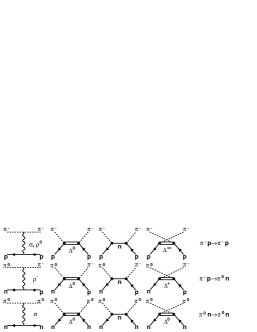
Рис. 2: Feynman diagrams for the $\pi^{-}p$ scattering.

Рис. 3: The $\Delta_{3}$ mass correction. Solid and dashed lines represent results of the present (NORDITA trom ) work.

Рис. 4: Energy–dependence of the phase–shifts difference $\delta^{++}_{33}(w)-\delta^{0}_{33}(w)$. Solid line shows the result of the present work. The dashed line corresponds to the case, when $g_{\pi^{+}p\Delta}$ is increased by 1% in comparison with the corresponding couplings for the other charged channels. Filled  abav and open  bugg circles represent results of previous partial–wave analyses.

Рис. 5: Energy dependence of the inelasticity parameter $\eta^{0}_{33}(w)$. Solid line shows result of the present work. Filled circles represent results (the uncertainties are within the symbols) from bugg .

Рис. 6: The energy dependence of the $S$– and $P$– phase–shifts. Solid lines show results of the present work. (a) $S_{11}$, (b) $S_{31}$, (c) $P_{11}$, (d) $P_{31}$, (e) $P_{13}$, and (f) $P_{33}$. The solid (open) circles are the GW SAID single–energy solutions associated with FA02 fa02 (Karlsruhe KH80 koch , the uncertainties are within the symbols).

Рис. 7: The differential cross sections for the $\pi^{-}p\to\pi^{0}n$ reaction. (a) $T_{\pi}=10.6$ MeV, (b) $T_{\pi}=20.6$ MeV, and (c) $T_{\pi}=39.4$ MeV. Solid line is the result of the present work. Solid circles represent data from isenh .

Рис. 8: The differential cross sections for the $\pi^{-}p\to\pi^{0}n$ reaction. (a) $T_{\pi}=64.1$ MeV, (b) $T_{\pi}=83.6$ MeV, (c) $T_{\pi}=95.1$ MeV, (d) $T_{\pi}=114.7$ MeV, (e) $T_{\pi}=136.0$ MeV, (f) $T_{\pi}=165.6$ MeV, (g) $T_{\pi}=189.4$ MeV, and (h) $T_{\pi}=212.1$ MeV. Line represents predictions of the present work. Solid circles are recent data from  mike .

. . , . , . . , . .

$K$- $\Delta-$
$\pi N$ .

$\pi N$– $T_{\pi}\leq$ 250  $K$– .

. $\pi^{+}-\pi^{0}$ $p-n$ NORDITA. . $\Delta^{0}$– and $\Delta^{++}$– . $\pi N$– – FA02 , , . ($\leq$1%) $T_{\pi}\sim 30-70$  , 7% , Gibbs . Matsinos, , .