Single Top Quark Production and Decay at Next-to-leading Order in Hadron Collision

Abstract

We present a calculation of the next-to-leading order QCD corrections, with one-scale phase space slicing method, to single top quark production and decay process $p\bar{p},pp\rightarrow t\bar{b}+X\rightarrow b\ell\nu\bar{b}+X$ at hadron colliders. Using the helicity amplitude method, the angular correlation of the final state partons and the spin correlation of the top quark are preserved. The effect of the top quark width is also examined.

I Introduction

At hadron colliders, the top quarks ($t$) are predominantly produced in pairs via the strong interaction process $q{\bar{q}},\,gg\rightarrow t\bar{t}$. Though it is possible to study the decay branching ratios of the top quark in $t\bar{t}$ pairs, to test the coupling of top quark with bottom quark ($b$) and $W$ gauge boson in hadron collisions, it is best to study the single-top quark production. Compared to the top quark pair production, produced by the interaction of the Quantum Chromodynamics (QCD), the single top quark productions are through the electroweak interaction connecting top quark to the down-type quarks, with amplitudes proportional to the Cabibbo-Kabayaashi-Maskawa (CKM) matrix elements. Due to the nature of left-handed charged weak current interaction, the top quark produced via single-top processes is highly polarized. Furthermore, top quark will decay via weak interaction before it has a chance to form a hadron, so its polarization property can be studied from the angular distributions of its decay particles. Hence, measuring the production rate of the single-top event can directly probe the electroweak properties of the top quark. For example, it can be used to measure the CKM matrix element $V_{tb}$ and to test the $V-A$ structure of the top quark charged-current weak interaction, or to probe CP violation effects Yuan:1994fn ; Atwood:1996pd ; Bar-Shalom:1997si . Besides of playing the role as a test of the Standard Model (SM), the precision measurement of the single top quark events has additional importance in searching for new physics, because the charged-current top quark coupling ($W$-$t$-$b$) might be particularly sensitive to certain new physics via new weak interactions or via loop effects, and new production mechanism might also contribute to the single top event rate Kane:1991bg ; Carlson:1994bg ; Rizzo:1995uv ; Malkawi:1996fs ; Tait:1996dv ; Datta:1996gg ; Li:1996ir ; Simmons:1996ws ; Whisnant:1997qu ; Baringer:1997wu ; Li:1997qf ; Tait:1997fe ; Hikasa:1998wx ; Han:1998tp ; He:1998ie ; Boos:1999dd ; Espriu:2001vj . Furthermore, the single-top event is also an important background to the search of Higgs boson ($q\bar{q}^{\prime}\rightarrow WH$ with $H\rightarrow b\bar{b}$) at the Tevatron Stange:1993ya ; Stange:1994bb ; Belyaev:1995gb and other new physics search Cao:2003tr .

Because of the unique features of the single top quark physics, it has been extensively studied in the literature Tait:1997fe ; Cortese:1991fw ; Stelzer:1995mi ; Mrenna:1997wp ; Willenbrock:1997nr ; Stelzer:1998ni ; Belyaev:1998dn ; Smith:1996ij ; Stelzer:1997ns ; Dawson:1984gx ; Willenbrock:1986cr ; Yuan:1989tc ; Ellis:1992yw ; Carlson:1993dt ; Heinson:1996zm ; Bordes:1994ki ; Ladinsky:1990ut ; Moretti:1997ng ; Tait:1999cf ; Belyaev:2000me ; Tait:2000sh ; Zhu:2001hw . There are three separate single top quark production processes of interest at the hadron collider, which may be characterized by the virtuality of the $W$ boson (with four momentum $q$) in the processes. The s-channel process $q\bar{q}^{\prime}\rightarrow W^{*}\rightarrow t\bar{b}$ via a virtual s-channel $W$ boson involves a timelike $W$ boson, $q^{2}>(m_{t}+m_{b})^{2}$, the t-channel process $qb\rightarrow q^{\prime}t$ (including $\bar{q}^{\prime}b\rightarrow\bar{qt}$, also referred as $W$-gluon fusion) involves a spacelike $W$ boson, $q^{2}<0$, and the $tW$ associated production process $bg\rightarrow tW^{-}$ involves an on-shell $W$ boson, $q^{2}=m_{W}^{2}$. Therefore, these three single top quark production mechanisms probe the charged-current interaction in different $q^{2}$ regions and are thus complementary to each other. Furthermore, they are sensitive to different new physics effects Tait:2000sh , and should be separately studied.

To improve the theoretical prediction on the single-top production rate, a next-to-leading-order (NLO) correction, at the order of $\alpha_{s}$, for the s- and t-channel processes has been carried out in Refs. Smith:1996ij ; Stelzer:1997ns ; Bordes:1994ki . This is similar to the study of the $O(\alpha_{s})$ correction to the top quark decay Jezabek:1994zv . Although the above studies provide the inclusive rate for single-top production, they cannot predict the event topology of the single-top event, which is crucial to confront the theory with experimental data in which some kinematical cuts are necessary to detect such an event. For that, Refs. Harris:2002md ; Sullivan:2004ie have calculated the differential cross section for on-shell single top quark production. However, NLO corrections to the top quark decay process were not included, nor the effects of the top quark width were considered. Since the top quark production and decay do not occur in isolation from each other, a theoretical study that includes both kinds of corrections is needed. A complete NLO calculation should include contribution from the production and the decay of the top quark, and the angular correlation among the final state particles should be calculated to analyze the polarization of the top quark. The $O(\alpha_{s})$ corrections to kinematic distributions may depend on the kinematic cuts and on the jet algorithm that must be implemented in the experiments. Therefore, it is necessary to obtain a fully differential calculation that can be used to study the kinematics of the final state particles.

In this theory paper, we present a NLO QCD calculation with the one-scale phase space slicing method, which treats consistently $O(\alpha_{s})$ corrections to both the production and the decay of the top quark in single top events. Our approach can give not only the inclusive total cross section, but also the various kinematical distributions of the final state particles, and provide a study on the top quark polarization at the NLO. Furthermore, since realistic kinematical cuts can be applied, our approach allows the experimentalists to compare their results directly with the theoretical predictions. In our study, we assume in all cases leptonic decays of the $W$ boson (for the sake of definiteness, we shall consider $W^{+}\rightarrow e^{+}\nu$; the lepton mass effects will be neglected throughout this paper). The phenomenological discussions will be given in our sequential papers pheno-schan .

The rest of this paper is organized as follows. In Sec. II, we outline the method of our calculation. In Sec. III, we present the Born level helicity amplitudes of the production and decay of single top quark. In Sec IV, we present the NLO helicity amplitudes of the production and decay of single top quark. The effective form factor approach is adopted in the calculation to generalize the application of our formalism to, for example, studying new physics effects. In Sec. V, we use the phase space slicing (PSS) method to calculate the effective form factors. To regularize divergencies in the calculation that involves the $\gamma_{5}$ matrix, both the dimensional regularization (DREG) 'tHooft:1972fi and the dimensional reduction (DRED) Bern:2002zk schemes are examined and their difference is shown in each individual form factor. In Sec. VI, we show how to assemble all the components discussed above to enumerate the NLO differential cross section of the single top quark. Finally, we give our conclusions in Sec. VII.

II Outline of the calculation

In this section we outline the method of our calculation whose details shall be presented in the following sections.

II.1 Narrow width approximation

In this work, the narrow width approximation (NWA) is used to study the production and decay of single top quark, in which the $O(\alpha_{s})$ corrections can be unambiguously assigned to either the single top quark production process or the top quark decay process. A finite top width will result in a new type of virtual NLO Feynman diagram in which a gluon line is connected from the anti-bottom quark (of the production process) to the bottom quark (of the decay process). Moreover, there will also be interference between the gluons emitted in the production and the gluon emitted in the decay if the effects of finite top quark width is considered. Those effects are nonfactorizable, which are similar to the effects of QED radiative corrections to the scattering process $e^{+}e^{-}\rightarrow W^{+}W^{-}\rightarrow 4f$. It was shown that the nonfactorizable effects are small as long as the process is not near the threshold Melnikov:1995fx ; Beenakker:1997ir ; Beenakker:1997bp . This provides the motivation of using the NWA for this kind of calculation Schmidt:1995mr ; Macesanu:2001bj ; Pittau:1996rp .

The single top quark can be produced through s-channel and t-channel processes, as shown in Fig. 1(a) and Fig. 1(b), respectively. Using the NWA, we decompose the Born level processes, depicted in Fig. 1 as indicated by symbol $\otimes$, into two parts: the top quark production and its sequential decay, where both the production and decay matrices are separately gauge invariant. Making use of the polarization information of the top quark, we can apply the NWA to correlate the top quark production with the top quark decay processes by replacing the numerator of the top quark propagator ($\hbox to0.0pt{/\hss}p_{t}+m_{t}$) by $\sum_{\lambda_{t}=\pm}u^{\lambda_{t}}(t)\bar{u}^{\lambda_{t}}(t)$. Here $u^{\lambda_{t}}(t)$ is the Dirac spinor of the top quark with helicity $\lambda_{t}$, where $\lambda_{t}=+$ or $-$ for a right-handed or left-handed top quark, respectively. Therefore, the scattering amplitude of the single top quark production and decay processes can be written as Kane:1991bg

$$\mathcal{M}=\sum_{\lambda_{t}=\pm}\mathcal{M}^{dec}(\lambda_{t})\mathcal{M}^{prod}(\lambda_{t}),$$ (1)

where $\mathcal{M}(\lambda_{t})$ is the helicity amplitude and $\lambda_{t}$ is the helicity eigenvalue of the single top quark produced in the intermediate state. The matrix element squared can be written as the product of the production part and the decay part in the density matrix formalism:

$$\left|\mathcal{M}\right|^{2}=\sum_{\lambda_{t},\lambda_{t}^{\prime}=\pm}\mathcal{A}_{\lambda_{t},\lambda_{t}^{\prime}}\mathcal{B}_{\lambda_{t},\lambda_{t}^{\prime}},$$ (2)

where

$$\mathcal{A}_{\lambda_{t},\lambda_{t}^{\prime}} = \mathcal{M}_{dec}^{\dagger}(\lambda_{t})\mathcal{M}_{dec}(\lambda_{t}^{\prime}),$$ (3)

$$\mathcal{B}_{\lambda_{t},\lambda_{t}^{\prime}} = \mathcal{M}_{prod}^{\dagger}(\lambda_{t})\mathcal{M}_{prod}(\lambda_{t}^{\prime}).$$ (4)

In addition to the matrix elements, the phase space of the single top quark processes can also be factorized into the top quark production and decay for an on-shell top quark in NWA by writing the denominator of the top quark propagator as

$$\int dp^{2}\frac{1}{(p^{2}-m_{t}^{2})^{2}+m_{t}^{2}\Gamma_{t}^{2}}=\frac{\pi}{m_{t}\Gamma_{t}}.$$ (5)

When the matrix element is calculated using the fixed $m_{t}$ value, it is the usual NWA method. In this case, the invariant mass of the top quark decay particles will be equal to $m_{t}$ (a fixed value) for all events. Reconstructing the top quark invariant mass from its decay particles is an important experimental task at the Tevatron and the LHC, it is desirable to have a theory calculation that would produce the invariant mass distribution of the reconstructed top quark mass with a Breit-Wigner resonance shape to reflect the non-vanishing decay width of the top quark (for being an unstable resonance). For that, we introduce the “modified NWA” method in our numerical calculation in which we generate a Breit-Wigner distribution for the top quark invariant mass in the phase space generator and then calculate the squared matrix element according to Eq. (2) with $m_{t}$ being the invariant mass generated by the phase space generator on the event-by-event basis. In the limit that the total decay width of the top quark approaches to zero (i.e., much smaller than the top quark mass), the production and the decay of top quark can be factorized. Therefore, the S-matrix element for the production and the decay processes are separately gauge invariant with any value of top quark invariant mass. We find that the total event rate and the distributions of various kinematics variables (except the distribution of the reconstructed top quark invariant mass) calculated using the “modified NWA” method agree well with that using the NWA method. In the NWA method, the reconstructed top quark invariant mass distribution is a delta-function, i.e., taking a fixed value, while in the “modified NWA” method, it is almost a Breit-Wigner distribution. The reason that the “modified NWA” method does not generate a perfect Breit-Wigner shape in the distribution of the top quark invariant mass is because the initial state parton luminosities (predominantly due to valence quarks) for the s-channel single-top process drop rapidly at the relevant Bjorken-$x$ range, where $\left\langle x\right\rangle\simeq\frac{m_{t}}{\sqrt{s}}\sim 0.1$.

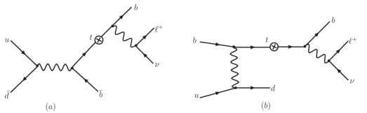
Figure 1: Feynman diagrams of the Born level contribution to the production and decay of single top quark. (a) s-channel (b) t-channel

II.2 Phase space slicing method

When calculating NLO QCD corrections, one generally encounters both ultraviolet (UV) and infrared (IR) (soft and collinear) divergencies. The former divergencies can be removed by proper renormalization of couplings and wave functions. We don’t need to renormalize the couplings in our calculation because the Born level couplings do not involve QCD interaction. In order to handle the latter divergencies, one has to consider both virtual and real corrections. The soft divergencies will cancel according to the Kinoshita-Lee-Nauenberg (KLN) theorem Kinoshita:1962ur ; Lee:1964is , but some collinear divergencies will remain uncanceled. In the case of considering the initial state partons, one needs to absorb additional collinear divergencies to define the NLO parton distribution function (PDF) of the initial state partons. After that, all the infrared-safe observables will be free of any singularities. To calculate the inclusive production rate, one can use the dimensional regularization scheme to regularize divergencies and adopt the modified minimal subtraction ($\overline{{\rm MS}}$) factorization scheme to obtain the total rate. However, owing to the complicated phase space for multi-parton configurations, analytic calculations are in practice impossible for all but the simplest quantities. During the last few years, effective numerical computational techniques have been developed to calculate the fully differential cross section to NLO and above. There are, broadly speaking, two types of algorithm used for NLO calculations: the phase space slicing method, and the dipole subtraction method Fabricius:1981sx ; Kramer:1986mc ; Giele:1991vf ; Giele:1993dj ; Keller:1998tf ; Ellis:1980wv ; Catani:1996jh ; Catani:1996vz ; Harris:2001sx ; Catani:2002hc . In this study, we use the phase space slicing method (PSS) with one cutoff scale for which the universal crossing functions have been derived in Ref. Giele:1993dj . The advantage of this method is that, after calculating the effective matrix elements with all the partons in the final state, we can use the generalized crossing property of the NLO matrix elements to calculate the corresponding s-channel or t-channel matrix elements numerically without requiring any further effort. The validity of this method is due to the property that both the phase space and matrix element of the initial and final state collinear radiation processes can be simultaneously factorized. Below, we briefly review the general formalism of the NLO calculation in PSS method with one cutoff scale.

The phase space slicing method with one cutoff scale introduces an unphysical parameter $s_{min}$ to separate the real emission correction phase space into two regions: (1) the resolved region in which the amplitude has no divergencies and can be integrated numerically by Monte Carlo method; (2) the unresolved region in which the amplitude contains all the soft and collinear divergencies and can be integrated out analytically. It should be emphasized that the notion of resolved/unresolved partons is unrelated to the physical jet resolution criterium or to any other relevant physical scale. In the massless case, a convenient definition of the resolved region is given by the requirement $s_{ij}>s_{min}$ for all invariants $s_{ij}=(p_{i}+p_{j})^{2}$, where $p_{i}$ and $p_{j}$ are the 4-momenta of partons $i$ and $j$, respectively. For the massive quarks, we follow the definition in Ref. Brandenburg:1997pu to account for masses, but still use the terminology “resolved” and “unresolved” partons. In the regions with unresolved partons, soft and collinear approximations of the matrix elements, which hold exactly in the limit $s_{min}\rightarrow 0$, are used. The necessary integrations over the soft and collinear regions of phase space can then be carried out analytically in $d=4-2\epsilon$ space-time dimensions. One can thus isolate all the poles in $\epsilon$ and perform the cancellation of the IR singularities between the real and virtual contributions and absorb the leftover singularities into the parton structure functions via the factorization procedure. After the above procedure, one takes the limit $\epsilon\rightarrow 0$. The contribution from the sum of virtual and unresolved region corrections is finite but $s_{min}$ dependent. Since the parameter $s_{min}$ is introduced in the theoretical calculation for technical reasons only and is unrelated to any physical quantity, the sum of all contributions (virtual, unresolved and resolved corrections) must not depend on $s_{min}$. We note that the phase space slicing method is only valid in the limit that $s_{{\rm min}}$ is small enough so that a given jet finding algorithm (or any infrared-safe observable) can be consistently defined even after including the experimental cuts.

In general, the conventional calculation of the NLO differential cross section for a process with initial state hadrons $H_{1}$ and $H_{2}$ can be written as

$$d\sigma_{H_{1}H_{2}}^{NLO}=\sum_{a,b}\int dx_{1}dx_{2}f_{a}^{H_{1}}(x_{1},\mu_{F})f_{b}^{H_{2}}(x_{2},\mu_{F})d\widehat{\sigma_{ab}^{NLO}}(x_{1,}x_{2},\mu_{R}),$$ (6)

where $a$, $b$ denote parton flavors and $x_{1}$, $x_{2}$ are parton momentum fractions. $f_{a}^{H}(x,\mu_{F})$ is the usual NLO parton distribution function with the mass factorization scale $\mu_{F}$ and $d\widehat{\sigma_{ab}^{NLO}}(x_{1},x_{2},\mu_{R})$ is the NLO hard scattering differential cross section with the renormalization scale $\mu_{R}$. The diagrammatic demonstration of Eq. (6) is shown in the upper part of Fig. 2.

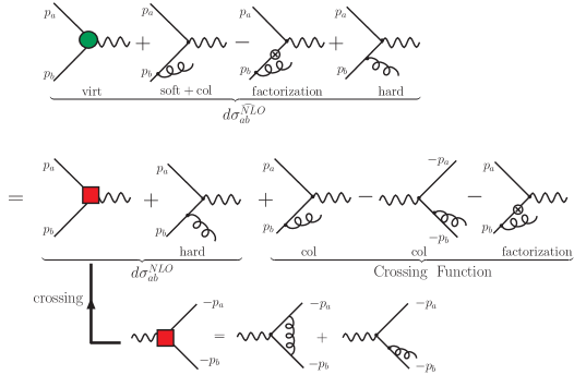
Figure 2: Illustration of the PSS method with one cutoff scale to describe the processes with initial state massless quarks. Here, only half of the real emission diagrams is shown. In this paper, we assign the particle’s momentum such that the initial state particle’s momentum is incoming to the vertex while the final state particle’s momentum is outgoing.

Unlike the conventional calculation method, the PSS method with one cutoff scale will first cross the initial state partons into the final state, including the virtual corrections and unresolved real emission corrections. For example, to calculate the s-channel single top quark production at the NLO, we first calculate the radiative corrections to $W^{*}\rightarrow q\bar{q}^{\prime}(g)$, as shown in the lower part of the Fig. 2, in which we split the phase space of the real emission corrections into the unresolved and resolved region. After we integrate out the unresolved phase space region, the net contribution of the virtual corrections and the real emission corrections in the unresolved phase space is finite but theoretical cutoff ($s_{min}$) dependent, and it can be written as a form factor (denoted by the box in Fig. 2) of the Born level vertex.

Secondly, we take the already calculated effective matrix elements with all the partons in the final state and use the universal “crossing function”, which is the generalization of the crossing property of the LO matrix elements to NLO, to calculate the corresponding matrix elements numerically. Once we cross the needed partons back to the initial state, the contributions from the unresolved collinear phase space regions are different from those with all the partons in the final state. These differences are included into the definition of the crossing function (including the mass factorization effects), as shown in the middle part of Fig. 2. In this paper, we only present the explicit expressions of the crossing function. For the definition and detailed derivation of the crossing function, we refer the reader to Ref. Giele:1993dj . After applying the mass factorization in a chosen scheme, the $s_{min}$ dependent crossing functions for an initial state parton $a$, which participates in the hard scattering processes, can be written in the form:

$$C_{a}^{{\rm scheme}}(x,\mu_{F},s_{min})=\left(\frac{N_{C}}{2\pi}\right)\left[A_{a}(x,\mu_{F})\log\left(\frac{s_{min}}{\mu_{F}}\right)+B_{a}^{{\rm scheme}}(x,\mu_{F})\right],$$ (7)

where

$$A_{a}(x,\mu_{F}) = \sum_{p}A_{p\rightarrow a}\left(x,\mu_{F}\right),$$ (8)

$$B_{a}^{{\rm scheme}}(x,\mu_{F}) = \sum_{p}B_{p\rightarrow a}^{{\rm scheme}}(x,\mu_{F}),$$ (9)

and $N_{C}$ denotes the number of colors. The sum runs over $p=q,\bar{q},g$. The functions $A$ and $B$ can be expressed as convolution integrals over the parton distribution functions and their explicit forms are shown in Appendix B. Although $A_{a}$ is scheme independent, $B_{a}$ does depend on the mass factorization scheme, and so does the crossing function.

After introducing the crossing function, we can write the NLO differential cross section in the PSS method with one cutoff scale as

$$d\sigma_{H_{1}H_{2}}^{NLO} = \sum_{a,b}\int dx_{1}dx_{2}\biggl{\{}f_{a}^{H_{1}}(x_{1},\mu_{F})f_{b}^{H_{2}}(x_{2},\mu_{F})d\sigma_{ab}^{NLO}(x_{1},x_{2},\mu_{R})$$

$$+ \alpha_{s}(\mu_{R})\biggl{[}C_{a}^{H_{1}}(x_{1},\mu_{F})f_{b}^{H_{2}}(x_{2},\mu_{F})+f_{a}^{H_{1}}(x_{1},\mu_{F})C_{b}^{H_{2}}(x_{2},\mu_{F})\biggr{]}d\sigma_{ab}^{LO}(x_{1},x_{2})\biggr{\}}.$$

Here $d\sigma_{ab}^{NLO}$ consists of the finite effective all-partons-in-the-final-state matrix elements, in which partons $a$ and $b$ have simply been crossed to the initial state, i.e. in which their momenta $-p_{a}$ and $-p_{b}$ have been replaced by $p_{a}$ and $p_{b}$, as shown in the Fig. 2. The difference between $d\sigma_{ab}^{NLO}$ and $d\widehat{\sigma_{ab}^{NLO}}$ has been absorbed into the finite, universal crossing function $C_{a}^{H}(x,\mu_{F})$. Defining an “effective” NLO parton distribution function $\mathcal{F}_{a}^{H}(x)$ as

$$\mathcal{F}_{a}^{H}(x)=f_{a}^{H}(x,\mu_{F})+\alpha_{s}(\mu_{R})C_{a}^{H}(x,\mu_{F})+O(\alpha_{s}^{2}),$$ (11)

we can rewrite Eq. (II.2) in a simple form as

$$d\sigma_{H_{1}H_{2}}^{NLO}=\sum_{a,b}\int dx_{1}dx_{2}\mathcal{F}_{a}^{H_{1}}(x_{1})\mathcal{F}_{b}^{H_{2}}(x_{2})d\sigma_{ab}^{NLO}(x_{1},x_{2}).$$ (12)

II.3 $\gamma_{5}$ problem

Because of the presence of the axial-vector current, a prescription to handle the $\gamma_{5}$ matrices in $d$($=4-2\epsilon$) dimensions has to be chosen. In this paper, we show the results of our calculations using both the dimensional regularization (DREG) scheme (’t Hooft-Veltman scheme 'tHooft:1972fi ) and the dimensional reduction (DRED) scheme (four dimensional helicity scheme Bern:2002zk ) to regulate the ultraviolet and infrared divergencies presented in the NLO calculations. We note that the results of form factors and the crossing function should be done consistently in a given scheme. Except for the top quark mass renormalization, we work in the $\overline{{\rm MS}}$ scheme throughout the paper to perform the needed renormalization and factorization procedures in order to calculate any ultraviolet and infrared finite physical observable. To renormalize the top quark mass, we use the on-shell subtraction scheme.

III Leading order results of single top quark production and decay process

In this section we present the leading order results of the single top quark processes. Using the density matrix method in the NWA, cf. Eq. (2), we factorize the s-channel and t-channel single top quark processes (cf. Fig. 1) into the top quark production and decay, separately. To compute the amplitudes we use the spinor helicity methods Berends:1981rb ; Kleiss:1985yh ; Xu:1986xb ; Gunion:1985vc ; Mangano:1990by with the conventions as in Ref. carlson , and for completeness, we briefly review the notation in Appendix A. We note that in some of Refs. Berends:1981rb ; Kleiss:1985yh ; Xu:1986xb ; Gunion:1985vc ; Mangano:1990by the phase conventions do not correspond to the helicity convention utilized in this paper. Below, we give the explicit Born level helicity amplitudes of the single top quark production and decay, respectively.

III.1 Helicity matrix elements of single top quark production

The helicity amplitudes for the s-channel single top quark production can be written as following:

$$\mathcal{M}_{s}^{prod}(\lambda_{t}=+) = 2\left<\hat{t}\!+\!|\hat{\bar{d}}+\right>\left<\hat{u}\!+\!|\hat{\bar{b}}-\right>\omega_{-}^{t},$$ (13)

$$\mathcal{M}_{s}^{prod}(\lambda_{t}=-) = 2\left<\hat{t}\!-\!|\hat{\bar{d}}+\right>\left<\hat{u}\!+\!|\hat{\bar{b}}-\right>\omega_{+}^{t},$$ (14)

where we have suppressed, for simplicity, the common factor ${\displaystyle\sqrt{2E_{u}}\sqrt{2E_{\bar{d}}}\sqrt{2E_{b}}}$, the coupling constants ${\displaystyle\left(\frac{g}{\sqrt{2}}\right)^{2}}$ and the propagator ${\displaystyle\frac{1}{s-m_{W}^{2}}}$ with $s=(p_{u}+p_{\bar{d}})^{2}$. Here, $g$ is the $SU(2)$ coupling constant, $m_{W}$ denotes the mass of $W$-boson, and $\omega_{\pm}^{t}=\sqrt{E_{t}\pm\left|\vec{p_{t}}\right|}$, where $E_{t}$ and $\vec{p_{t}}$ are the energy and momentum of the top quark, respectively. The meaning of the bra ($<\mid$) and ket ($\mid>$) in the above helicity amplitudes is summarized in Appendix A. We note that $\hat{u},\hat{\bar{d}},\hat{t}$ and $\hat{\bar{b}}$ within the bra and ket denote the normalized three-momentum of the particle, cf. Eq. (155). We did not write explicitly the helicity states of the other massless quarks because only one set of the helicity states give a nonvanishing matrix element. For example, in this case the incoming $u$-quark is left-handed, $\bar{d}$ is right-handed and $\bar{b}$ is right-handed. To calculate the squared matrix element, one also needs to include the proper spin and color factors which are not explicitly shown in this paper.

For the t-channel single top quark production process, the helicity amplitudes are given by

$$\mathcal{M}_{t}^{prod}(\lambda_{t}=+) = 2\left<\hat{u}\!+\!|\hat{b}-\right>\left<\hat{t}\!+\!|\hat{d}+\right>\omega_{-}^{t},$$ (15)

$$\mathcal{M}_{t}^{prod}(\lambda_{t}=-) = 2\left<\hat{u}\!+\!|\hat{b}-\right>\left<\hat{t}\!-\!|\hat{d}+\right>\omega_{+}^{t},$$ (16)

where we have also suppressed the common factor ${\displaystyle\sqrt{2E_{u}}\sqrt{2E_{d}}\sqrt{2E_{b}}}$, the coupling constants ${\displaystyle\left(\frac{g}{\sqrt{2}}\right)^{2}}$, and the propagator ${\displaystyle\frac{1}{t-m_{W}^{2}}}$ with $t=(p_{u}-p_{d})^{2}$.

III.2 Helicity matrix elements of top quark decay

For the top quark decay process, the helicity amplitude are given by

$$\mathcal{M}^{dec}(\lambda_{t}=+) = -2\left<\hat{b^{\prime}}\!-\!|\hat{\nu}+\right>\left<\hat{e}\!+\!|\hat{t}+\right>\omega_{-}^{t},$$ (17)

$$\mathcal{M}^{dec}(\lambda_{t}=-) = -2\left<\hat{b^{\prime}}\!-\!|\hat{\nu}+\right>\left<\hat{e}\!+\!|\hat{t}-\right>\omega_{+}^{t},$$ (18)

where we only consider the leptonic decay mode of $W$ boson and suppress, for simplicity, the common factor ${\displaystyle\sqrt{2E_{e}}\sqrt{2E_{\nu}}\sqrt{2E_{b^{\prime}}}}$, the coupling constants ${\displaystyle\left(\frac{g}{\sqrt{2}}\right)^{2}}$, and the propagator ${\displaystyle\frac{1}{(p_{W}^{2}-m_{W}^{2})+im_{W}\Gamma_{W}}}$, where $p_{W}$ and $\Gamma_{W}$ are the 4-momenta and the total decay width of $W$-boson, respectively. All through out this paper we use $b^{\prime}$ to denote the bottom quark from top decay.

IV NLO matrix elements of Single top quark production and decay processes

Beyond the leading order, an additional gluon can be radiated from the quark lines or appear as the initial parton in the single top quark process . Since the single top quark can only be produced through the electroweak interaction in the SM, we can further separate the single top quark processes into smaller gauge invariant sets, even at the NLO. Taking advantage of this property, in the first part of this section we separate the s-channel and t-channel single top quark processes into smaller gauge invariant sets of diagrams to organize our calculations. As we pointed out in Sec. II.2, NLO QCD corrections in the PSS method can be separated into two parts: (I) the resolved real emission corrections and (II) the virtual correction plus the unresolved real (soft+collinear) emission corrections, denoted by “SCV”. After integrating out the virtual gluon and the unresolved partons, the SCV corrections can be written as form factors multiplying the Born level vertex. The form factors either modify the Born level coupling or give rise to new Lorentz structure of $W$ coupling to fermions. In the second part of this section, we will write down the most general form factors of the single top quark processes and show their contribution to the helicity amplitudes for both s-channel and t-channel processes explicitly. It is worthwhile to mention that the form factor formalism presented here can be easily extended to study new physics models whose effects also show up as form factors. The derivation of the form factors for single top quark production and decay processes as predicted by the SM can be found in the second part of this section. The resolved corrections are also calculated using helicity amplitude method and the results are shown in the third part of this section.

IV.1 Categorizing the single top quark processes

Here, we separate the NLO s-channel and t-channel single top quark processes into smaller gauge invariant sets of diagrams to organize our calculations. The NLO s-channel diagrams consist of all the virtual correction diagrams as well as the Feynman diagrams of the following real correction processes:

$$q\bar{q}^{\prime}\rightarrow W^{*}g\rightarrow\bar{b}gt(\rightarrow bW^{+}),$$ (19)

$$qg\rightarrow W^{*}q^{\prime}\rightarrow\bar{b}q^{\prime}t(\rightarrow bW^{+}),$$ (20)

$$g\bar{q}^{\prime}\rightarrow W^{*}\bar{q}\rightarrow\bar{b}\bar{q}t(\rightarrow bW^{+}),$$ (21)

$$q\bar{q}^{\prime}\rightarrow W^{*}\rightarrow\bar{b}gt(\rightarrow bW^{+}),$$ (22)

$$q\bar{q}^{\prime}\rightarrow W^{*}\rightarrow\bar{b}t(\rightarrow bW^{+}g),$$ (23)

where the gluon is connected only to ($q,q^{\prime}$) lines in (19)-(21), and the gluon connected only to ($t,\bar{b}$) lines in (22) and the gluon connected only to ($t,b$) lines in (23). We note that diagrams (20) and (21) do not include those in which the gluon line is connected to the final state $\bar{b}$ and $t$ line, for those are part of the NLO corrections to t-channel process as shown in Eqs. (26) and (27). To facilitate the presentation of our calculation, we separate the s-channel higher order QCD corrections (including both virtual and real corrections) into the following three categories:

• corrections to the initial state of the s-channel single top quark production (INIT), in which the gluon is only connected to the initial state light quark ($q,\bar{q}^{\prime}$) line,

• corrections to the final state of the s-channel single top quark production (FINAL), in which the gluon is only connected to the final state heavy quark ($t,\bar{b}$) line of the single top quark production,

• corrections to the decay of the top quark (SDEC), in which the gluon is connected to the heavy quark ($t,b$) line of the top quark decay.

The three types of corrections are illustrated in the upper part of Fig. 3, in which the blobs represent the higher order QCD corrections. The explicit real emission diagrams for the s-channel process can be found in Fig. 4.

The NLO t-channel real correction processes for the top quark production and decay are

$$bq\rightarrow q^{\prime}gt(\rightarrow bW^{+}),$$ (24)

$$b\bar{q}^{\prime}\rightarrow\bar{q}gt(\rightarrow bW^{+}),$$ (25)

$$qg\rightarrow q^{\prime}\bar{b}t(\rightarrow bW^{+}),$$ (26)

$$\bar{q}^{\prime}g\rightarrow\bar{q}\bar{b}t(\rightarrow bW^{+}),$$ (27)

$$bg\rightarrow\bar{q}q^{\prime}t(\rightarrow bW^{+}),$$ (28)

$$bq\rightarrow q^{\prime}t(\rightarrow bW^{+}g),$$ (29)

$$b\bar{q}^{\prime}\rightarrow\bar{q}t(\rightarrow bW^{+}g).$$ (30)

Here the gluon is connected to both ($q,q^{\prime}$) lines and ($t,\bar{b}$) lines in (24, 25), but only to ($t,b$) lines in (26, 27). In (28), we restrict the gluon to be connected only to ($q,q^{\prime}$) lines. When the gluon in (28) is connected to ($t,b$) lines, it corresponds to the process $bg\rightarrow tW$ with $W\rightarrow\bar{q}q^{\prime}$, therefore it is not included here. As done in the s-channel case, we separate the t-channel NLO QCD corrections (including both virtual and real corrections)(24-30) into three categories. As illustrated in the lower part of Fig. 3, they are:

• the one in which the gluon is connected to the light quark ($q,q^{\prime}$) lines (LIGHT),

• the one in which the gluon is connected to the heavy quark ($t,\bar{b}$) lines (HEAVY),

• the one in which the gluon is radiated from the heavy quark ($t,b$) lines of the on-shell top quark decay processes (TDEC),

The explicit real emission diagrams for the t-channel process can be found in Fig. 5.

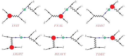
Figure 3: The way we organize our calculations at the NLO. The blobs in the diagrams denote the higher order QCD corrections, including both virtual and real emission contributions.

IV.2 Form factor formalism for SCV corrections

Below, we present the form factor formalism for each category defined in Sec. IV.1, after including both the virtual and unresolved real corrections.

IV.2.1 INIT form factors

Higher order QCD corrections to the diagrams labeled as INIT in Fig. 3 do not change the Lorentz structure of the $W^{*}-u-d$ coupling, therefore the most general form of the initial state contribution can be rewritten as

$$\frac{ig}{\sqrt{2}}\gamma^{\mu}P_{L}I_{L},$$ (31)

where $I_{L}$ denotes the effective form factor that includes the higher order corrections. Denoting the helicity amplitude as $\mathcal{M}_{INIT}(\lambda_{t})$ with top quark helicity $\lambda_{t}=\pm 1$ and suppressing, for simplicity, the common factor $\sqrt{2E_{u}}\sqrt{2E_{d}}\sqrt{2E_{\bar{{b}}}}$, the coupling factors $\left({\displaystyle\frac{g}{\sqrt{2}}}\right)^{2}$ and the propagators ${\displaystyle\frac{1}{s-m_{W}^{2}}}$ with $s=(p_{u}+p_{\bar{d}})^{2}$, we obtain the helicity amplitudes which include higher order corrections to the initial state of the s-channel single top quark production as following:

$$\mathcal{M}_{INIT}(+) = 2I_{L}\left<\hat{t}\!+\!|\hat{\bar{d}}+\right>\left<\hat{u}\!+\!|\hat{\bar{{b}}}-\right>\omega_{-}^{t},$$ (32)

$$\mathcal{M}_{INIT}(-) = 2I_{L}\left<\hat{t}\!-\!|\hat{\bar{d}}+\right>\left<\hat{u}\!+\!|\hat{\bar{{b}}}-\right>\omega_{+}^{t},$$ (33)

where $\omega_{\pm}^{t}=\sqrt{E_{t}\pm|\overrightarrow{p_{t}}|}$, cf. Appendix A.

Needless to say, when calculating the scattering amplitude of the single top quark production and decay process, cf. Eq. (1), up to the NLO, the decay matrix elements in this case is taken to be the Born level ones as given in Eqs. (13) and (14).

IV.2.2 FINAL form factors

In the limit that the bottom quark mass is taken to be zero , the most general $W^{\star}-t-b$ coupling, labeled as FINAL in Fig. 3, is

$$\frac{ig}{\sqrt{2}}\left\{\gamma_{\mu}(F_{1}^{L*}P_{L}+F_{1}^{R*}P_{R})-\frac{(t_{\mu}-\bar{b}_{\mu})}{m_{W}}(F_{2}^{R*}P_{L}+F_{2}^{L*}P_{R})\right\},$$ (34)

where the asterisk in the superscript of the form factors indicates taking its complex conjugate. This is different from the coupling in Eq. (31) because the top quark mass is kept in the calculation,and only the bottom quark mass is taken to be zero. Because the charged current interacts with massless quarks in the initial state, one can use the on-shell condition of the massless initial state quarks to rewrite Eq. (34) as

$$\frac{ig}{\sqrt{2}}\left\{\gamma_{\mu}(F_{1}^{L*}P_{L}+F_{1}^{R*}P_{R})+\bar{b}_{\mu}(F_{2}^{R*}P_{L}+F_{2}^{L*}P_{R})\right\},$$ (35)

where the $m_{W}$ has been absorbed into form factors $F_{2}^{R*}$ and $F_{2}^{L*}$. Denoting the helicity amplitude as $\mathcal{M}_{FINAL}(\lambda_{\bar{b}},\lambda_{t})$, we obtain the helicity amplitudes which include higher order corrections to the s-channel single top quark production as following:

$$\mathcal{M}_{FINAL}(-,-) = 2F_{1}^{L*}\left<\hat{t}\!-\!|\hat{\bar{d}}+\right>\left<\hat{u}\!+\!|\hat{\bar{b}}-\right>\omega_{+}^{t}+F_{2}^{R*}\left<\!\hat{\bar{d}}\!-\!|\not\!\bar{b}|\hat{u}-\right>\left<\hat{t}\!-\!|\hat{\bar{b}}-\right>\omega_{-}^{t},$$ (36)

$$\mathcal{M}_{FINAL}(+,-) = 2F_{1}^{R*}\left<\hat{t}\!-\!|\hat{u}-\right>\left<\hat{\bar{d}}\!-\!|\hat{\bar{b}}+\right>\omega_{-}^{t}+F_{2}^{L*}\left<\!\hat{\bar{d}}\!-\!|\not\!\bar{b}|\hat{u}-\right>\left<\hat{t}\!-\!|\hat{\bar{b}}+\right>\omega_{+}^{t},$$ (37)

$$\mathcal{M}_{FINAL}(-,+) = 2F_{1}^{L*}\left<\hat{t}\!+\!|\hat{\bar{d}}+\right>\left<\hat{u}\!+\!|\hat{\bar{b}}-\right>\omega_{-}^{t}+F_{2}^{R*}\left<\!\hat{\bar{d}}\!-\!|\not\!\bar{b}|\hat{u}-\right>\left<\hat{t}\!+\!|\hat{\bar{b}}-\right>\omega_{+}^{t},$$ (38)

$$\mathcal{M}_{FINAL}(+,+) = 2F_{1}^{R*}\left<\hat{t}\!+\!|\hat{u}-\right>\left<\hat{\bar{d}}\!-\!|\hat{\bar{b}}+\right>\omega_{+}^{t}+F_{2}^{L*}\left<\!\hat{\bar{d}}\!-\!|\not\!\bar{b}|\hat{u}-\right>\left<\hat{t}\!+\!|\hat{\bar{b}}+\right>\omega_{-}^{t}.$$ (39)

As before, we have suppressed the common factor $\sqrt{2E_{u}}\sqrt{2E_{d}}\sqrt{2E_{\bar{{b}}}}$, the coupling factors $\left({\displaystyle\frac{g}{\sqrt{2}}}\right)^{2}$, and the propagators ${\displaystyle\frac{1}{s-m_{W}^{2}}}$ with $s=(p_{u}+p_{\bar{d}})^{2}$.

IV.2.3 LIGHT form factors

The effective form factor for $u-W^{*}-d$, labeled as LIGHT in Fig. 3, takes the exact same form as $W^{*}-u-d$ in Eq. (31). Hence, the helicity amplitudes $\mathcal{M}_{LIGHT}(\lambda_{t})$ for the t-channel single top quark production are given as follows:

$$\mathcal{M}_{LIGHT}(+) = 2L_{L}\left<\hat{t}\!+\!|\hat{d}+\right>\left<\hat{u}\!+\!|\hat{b}-\right>\omega_{-}^{t},$$ (40)

$$\mathcal{M}_{LIGHT}(-) = 2L_{L}\left<\hat{t}\!-\!|\hat{d}+\right>\left<\hat{u}\!+\!|\hat{b}-\right>\omega_{+}^{t},$$ (41)

where $L_{L}$ is the effective coupling induced by higher order corrections. Again, we have suppressed the common factor $\sqrt{2E_{u}}\sqrt{2E_{d}}\sqrt{2E_{b}}$, the coupling factors $\left({\displaystyle\frac{g}{\sqrt{2}}}\right)^{2}$ and the propagators ${\displaystyle\frac{1}{t-m_{W}^{2}}}$ with $t=(p_{u}-p_{d})^{2}$.

IV.2.4 HEAVY form factors

The effective form factor for $b-W^{*}-t$, labeled as HEAVY in Fig. 3, takes the exact same form as $W^{*}-t-b$ in Eq. (35). Hence, the helicity amplitudes $\mathcal{M}_{HEAVY}(\lambda_{b},\lambda_{t})$ for the t-channel single top quark production are given as follows:

$$\mathcal{M}_{HEAVY}(-,-) = 2H_{1}^{L*}\left<\hat{t}\!-\!|\hat{d}+\right>\left<\hat{u}\!+\!|\hat{b}-\right>\omega_{+}^{t}-H_{2}^{R*}\left<\!\hat{d}\!-\!|\not\!b|\hat{u}-\right>\left<\hat{t}\!-\!|\hat{b}-\right>\omega_{-}^{t},$$ (42)

$$\mathcal{M}_{HEAVY}(+,-) = 2H_{1}^{R*}\left<\hat{t}\!-\!|\hat{u}-\right>\left<\hat{d}\!-\!|\hat{b}+\right>\omega_{-}^{t}-H_{2}^{L*}\left<\!\hat{d}\!-\!|\not\!b|\hat{u}-\right>\left<\hat{t}\!-\!|\hat{b}+\right>\omega_{+}^{t},$$ (43)

$$\mathcal{M}_{HEAVY}(-,+) = 2H_{1}^{L*}\left<\hat{t}\!+\!|\hat{d}+\right>\left<\hat{u}\!+\!|\hat{b}-\right>\omega_{-}^{t}-H_{2}^{R*}\left<\!\hat{d}\!-\!|\not\!b|\hat{u}-\right>\left<\hat{t}\!+\!|\hat{b}-\right>\omega_{+}^{t},$$ (44)

$$\mathcal{M}_{HEAVY}(+,+) = 2H_{1}^{R*}\left<\hat{t}\!+\!|\hat{u}-\right>\left<\hat{d}\!-\!|\hat{b}+\right>\omega_{+}^{t}-H_{2}^{L*}\left<\!\hat{d}\!-\!|\not\!b|\hat{u}-\right>\left<\hat{t}\!+\!|\hat{b}+\right>\omega_{-}^{t},$$ (45)

where $H_{1,2}^{L,R}$ denote the effective couplings induced by higher order corrections. Here, we have suppressed the common factor $\sqrt{2E_{u}}\sqrt{2E_{d}}\sqrt{2E_{b}}$, the coupling factors $\left({\displaystyle\frac{g}{\sqrt{2}}}\right)^{2}$ and the propagators ${\displaystyle\frac{1}{t-m_{W}^{2}}}$ with $t=(p_{u}-p_{d})^{2}$.

IV.2.5 Top quark decay form factors

The most general $t-b-W$ coupling, labeled as DEC for both s-channel and t-channel processes, is

$$\frac{ig}{\sqrt{2}}\left\{\gamma_{\mu}(D_{1}^{L}P_{L}+D_{1}^{R}P_{R})-b_{\mu}^{\prime}(D_{2}^{R}P_{R}+D_{2}^{L}P_{L})\right\},$$ (46)

where $D_{1,2}^{L,R}$ denote the form factors which include higher order QCD corrections. Denoting the helicity amplitude as $\mathcal{M}_{DEC}(\lambda_{t},\lambda_{b^{\prime}})$, we obtain the helicity amplitudes which include higher order corrections to single top quark decay process as following:

$$\mathcal{M}_{DEC}(-,-) = -2D_{1}^{L}\left<\hat{b^{\prime}}\!-\!|\hat{\nu}+\right>\left<\hat{e}\!+\!|\hat{t}-\right>\omega_{+}^{t}+D_{2}^{R}\left<\!\hat{\nu}\!-\!|\not\!b^{\prime}|\hat{e}-\right>\left<\hat{b^{\prime}}\!-\!|\hat{t}-\right>\omega_{-}^{t},$$ (47)

$$\mathcal{M}_{DEC}(+,-) = -2D_{1}^{L}\left<\hat{b^{\prime}}\!-\!|\hat{\nu}+\right>\left<\hat{e}\!+\!|\hat{t}+\right>\omega_{-}^{t}+D_{2}^{R}\left<\!\hat{\nu}\!-\!|\not\!b^{\prime}|\hat{e}-\right>\left<\hat{b^{\prime}}\!-\!|\hat{t}+\right>\omega_{+}^{t},$$ (48)

$$\mathcal{M}_{DEC}(-,+) = -2D_{1}^{R}\left<\hat{b^{\prime}}\!+\!|\hat{e}-\right>\left<\hat{\nu}\!-\!|\hat{t}-\right>\omega_{-}^{t}+D_{2}^{L}\left<\!\hat{\nu}\!-\!|\not\!b^{\prime}|\hat{e}-\right>\left<\hat{b^{\prime}}\!+\!|\hat{t}-\right>\omega_{+}^{t},$$ (49)

$$\mathcal{M}_{DEC}(+,+) = -2D_{1}^{R}\left<\hat{b^{\prime}}\!+\!|\hat{e}-\right>\left<\hat{\nu}\!-\!|\hat{t}+\right>\omega_{+}^{t}+D_{2}^{L}\left<\!\hat{\nu}\!-\!|\not\!b^{\prime}|\hat{e}-\right>\left<\hat{b^{\prime}}\!+\!|\hat{t}+\right>\omega_{-}^{t},$$ (50)

where we ignore the common factor ${\displaystyle\sqrt{2E_{e}}\sqrt{2E_{\nu}}\sqrt{2E_{b^{\prime}}}}$, the coupling factors $\left({\displaystyle\frac{g}{\sqrt{2}}}\right)^{2}$ and the propagator ${\displaystyle\frac{1}{(p_{W}^{2}-m_{W}^{2})+im_{W}\Gamma_{W}}}$ with $p_{W}=p_{e^{+}}+p_{\nu}$.

The category SDEC (or TDEC) in Fig. 3 is obtained by convoluting the s-channel (or t-channel) Born level helicity amplitudes, cf. Eqs. (13) and (14) (or Eqs. (15) and (16)), with the corresponding DEC amplitudes listed above.

IV.3 Helicity amplitudes of resolved contributions

Here, we present the helicity amplitudes of resolved corrections for each category defined in Sec. IV.1.

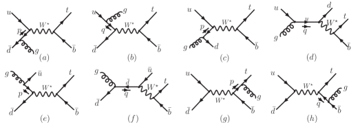
Figure 4: Feynman diagrams of the real emission corrections to s-channel single top quark production.

IV.3.1 NLO corrections to INIT

The Feynman diagrams of the initial state real emission corrections are shown in Figs. 4(a)-(f). At the NLO, a hard gluon can be radiated from the initial state quark line, or a quark can be generated from the gluon splitting. We separate the NLO INIT real emission corrections into three categories:

$${\rm INI-A} : q\bar{q}^{\prime}\rightarrow W^{*}g\rightarrow t\bar{b}g,\qquad{\rm including\,\,(a)\,\,and\,\,(b)},$$

$${\rm INI-B} : qg\rightarrow W^{*}q^{\prime}\rightarrow t\bar{b}q^{\prime},\quad\,\,\,\,\,{\rm including\,\,(c)\,\,and\,\,(d),}$$

$${\rm INI-C} : \bar{q}^{\prime}g\rightarrow W^{*}\bar{q}\rightarrow t\bar{b}\bar{q},\qquad{\rm including\,\,(e)\,\,and\,\,(f),}$$

which are separately gauge invariant. Denoting the helicity amplitude as $\mathcal{M}_{INI}^{A,B,C}(\lambda_{t})$, we calculate the helicity amplitudes for a given helicity state ($\lambda_{t}$) of the top quark, which are listed as follows.

The helicity amplitudes for INI A are :

$$\mathcal{M}_{INI}^{A}(+) = 2\,\omega_{-}^{t}\left\{-\frac{\left<\hat{\bar{d}}\!-\!|\hat{t}-\right>\left<\hat{\bar{b}}\!\!+\!|\not{\!p}_{-}\not{\!\varepsilon^{*}}_{+}|\hat{u}-\right>}{p^{2}}+\frac{\left<\hat{\bar{b}}\!+\!|\hat{u}-\right>\left<\hat{\bar{d}}\!-\!|\not{\!\varepsilon^{*}}_{+}\not{\!q}_{-}|\hat{u}-\right>}{q^{2}}\right\},$$ (51)

$$\mathcal{M}_{INI}^{A}(-) = 2\,\omega_{+}^{t}\left\{\frac{\left<\hat{\bar{d}}\!-\!|\hat{t}+\right>\left<\hat{\bar{b}}\!\!+\!|\not{\!q}_{-}\not{\!\varepsilon^{*}}_{+}|\hat{u}-\right>}{p^{2}}-\frac{\left<\hat{\bar{b}}\!+\!|\hat{u}-\right>\left<\hat{\bar{d}}\!-\!|\not{\!\varepsilon^{*}}_{+}\not{\!q}_{-}|\hat{t}+\right>}{q^{2}}\right\},$$ (52)

with $p=p_{u}-p_{g}$ and $q=p_{\bar{d}}-p_{g}$.

The helicity amplitudes for INI B are :

$$\mathcal{M}_{INI}^{B}(+) = 2\,\omega_{-}^{t}\left\{-\frac{\left<\hat{\bar{b}}\!+\!|\hat{u}-\right>\left<\hat{d}\!-\!|\not{\!\varepsilon}_{+}\not{\!p}_{-}|\hat{t}-\right>}{p^{2}}+\frac{\left<\hat{d}\!-\!|\hat{t}-\right>\left<\hat{\bar{b}}\!\!+\!|\not{\!q}_{-}\not{\!\varepsilon}_{+}|\hat{u}-\right>}{q^{2}}\right\},$$ (53)

$$\mathcal{M}_{INI}^{B}(-) = 2\,\omega_{+}^{t}\left\{-\frac{\left<\hat{\bar{b}}\!+\!|\hat{u}-\right>\left<\hat{\bar{d}}\!-\!|\not{\!\varepsilon}_{+}\not{\!p}_{-}|\hat{t}+\right>}{p^{2}}+\frac{\left<\hat{d}\!-\!|\hat{t}+\right>\left<\hat{\bar{b}}\!\!+\!|\not{\!q}_{-}\not{\!\varepsilon}_{+}|\hat{u}-\right>}{q^{2}}\right\},$$ (54)

with $p=p_{g}-p_{d}$ and $q=p_{g}+p_{u}$.

The helicity amplitudes for INI C are :

$$\mathcal{M}_{INI}^{C}(+) = 2\,\omega_{-}^{t}\left\{-\frac{\left<\hat{\bar{b}}\!+\!|\hat{\bar{u}}-\right>\left<\hat{\bar{d}}\!-\!|\not{\!\varepsilon}_{+}\not{\!q}_{-}|\hat{t}-\right>}{q^{2}}+\frac{\left<\hat{\bar{d}}\!-\!|\hat{t}-\right>\left<\hat{\bar{b}}\!\!+\!|\not{\!p}_{-}\not{\!\varepsilon}_{+}|\hat{\bar{u}}-\right>}{p^{2}}\right\},$$ (55)

$$\mathcal{M}_{INI}^{C}(-) = 2\,\omega_{+}^{t}\left\{-\frac{\left<\hat{\bar{b}}\!+\!|\hat{\bar{u}}-\right>\left<\hat{\bar{d}}\!-\!|\not{\!\varepsilon}_{+}\not{\!q}_{-}|\hat{t}+\right>}{q^{2}}+\frac{\left<\hat{\bar{d}}\!-\!|\hat{t}+\right>\left<\hat{\bar{b}}\!\!+\!|\not{\!p}_{-}\not{\!\varepsilon}_{+}|\hat{\bar{u}}-\right>}{p^{2}}\right\},$$ (56)

with $p=p_{g}-p_{\bar{u}}$ and $q=p_{g}+p_{\bar{d}}$.

Again in all the above equations, we have suppressed the common factor $\sqrt{2E_{u}}\sqrt{2E_{\bar{d}}}\sqrt{2E_{\bar{b}}}$, the coupling factors ${\displaystyle g_{s}\left(\frac{g}{\sqrt{2}}\right)^{2}}$, and the propagator ${\displaystyle\frac{1}{p_{W}^{2}-m_{W}^{2}+im_{W}\Gamma_{W}}}$ with $p_{W}=p_{t}+p_{\bar{b}}$. Here, $g_{s}$ is the coupling constant of the strong interaction.

IV.3.2 NLO corrections to FINAL

The Feynman diagrams for NLO real emission corrections to the final state of s-channel top quark production process are shown in the Fig. 4(g) and (h). Denoting the helicity amplitude as $\mathcal{M}_{FINAL}(\lambda_{t})$, then

$$\mathcal{M}_{FINAL}(+) = 2\,\omega_{-}^{t}\frac{\left<\hat{u}\!+\!|\hat{\bar{b}}-\right>\left<\hat{t}\!+\!|\not{\!\varepsilon^{*}}_{+}\not{\!p}_{-}|\hat{\bar{d}}+\right>}{p^{2}-m_{t}^{2}}+2\,m_{t}\>\omega_{+}^{t}\frac{\left<\hat{u}\!+\!|\hat{\bar{b}}-\right>\left<\hat{t}\!\!+\!|\!\not{\!\varepsilon^{*}}_{-}|\hat{\bar{d}}+\right>}{p^{2}-m_{t}^{2}}$$ (57)

$$- 2\,\omega_{-}^{t}\frac{\left<\hat{t}\!+\!|\hat{\bar{d}}+\right>\left<\hat{u}\!\!+\!|\not{\!q}_{-}\not{\!\varepsilon^{*}}_{+}|\hat{\bar{b}}-\right>}{q^{2}},$$

$$\mathcal{M}_{FINAL}(-) = 2\,\omega_{+}^{t}\frac{\left<\hat{u}\!+\!|\hat{\bar{b}}-\right>\left<\hat{t}\!-\!|\not{\!\varepsilon^{*}}_{+}\not{\!p}_{-}|\hat{\bar{d}}+\right>}{p^{2}-m_{t}^{2}}+2\,m_{t}\,\omega_{-}^{t}\frac{\left<\hat{u}\!+\!|\hat{\bar{b}}-\right>\left<\!\,\hat{t}\!-\!|\not{\!\varepsilon^{*}}_{-}|\hat{\bar{d}}+\right>}{p^{2}-m_{t}^{2}}$$ (58)

$$- 2\,\omega_{+}^{t}\frac{\left<\hat{t}\!-\!|\hat{\bar{d}}+\right>\left<\hat{u}\!\!+\!|\not{\!q}_{-}\not{\!\varepsilon^{*}}_{+}|\hat{\bar{b}}-\right>}{q^{2}},$$

with $p=p_{g}+p_{t}$ and $q=p_{g}+p_{\bar{b}}$. We again suppressed the common factor $\sqrt{2E_{u}}\sqrt{2E_{\bar{d}}}\sqrt{2E_{\bar{b}}}$, the coupling constants ${\displaystyle g_{s}\left(\frac{g}{\sqrt{2}}\right)^{2}}$, and the $W$ boson propagator ${\displaystyle\frac{1}{p_{W}^{2}-m_{W}^{2}+im_{W}\Gamma_{W}}}$ with $p_{W}=p_{u}+p_{\bar{d}}$.

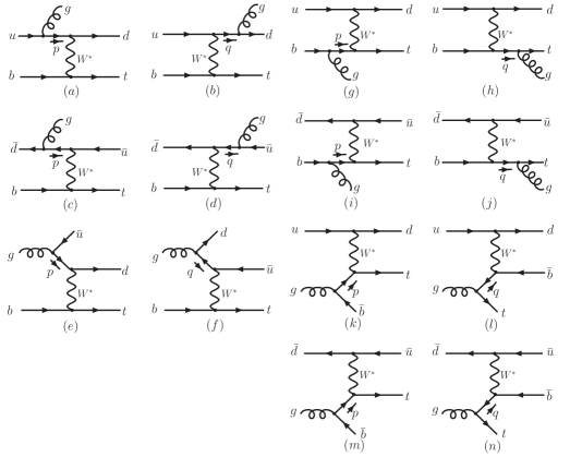
Figure 5: Feynman diagrams of the real emission corrections to the t-channel single top quark production

IV.3.3 NLO corrections to LIGHT

The Feynman diagrams, that generate real emission contributions through coupling a gluon to the light quark lines, are shown in Figs. 5(a) to (f). To facilitate our calculations, we separate the NLO LIGHT real emission corrections into the following three categories:

$${\rm LIGHT-A} : bq\rightarrow q^{\prime}gt,\qquad{\rm including\,\,(a)\,\,and\,\,(b),}$$

$${\rm LIGHT-B} : b\bar{q}^{\prime}\rightarrow\bar{q}gt,\qquad{\rm including\,\,(c)\,\,and\,\,(d),}$$

$${\rm LIGHT-C} : bg\rightarrow\bar{q}q^{\prime}t.\qquad{\rm\,including\,\,(e)\,\,and\,\,(f).}$$

Denoting the helicity amplitude as $\mathcal{M}_{LIGHT}^{A,B,C}(\lambda_{t})$, then the helicity amplitudes for LIGHT-A are:

$$\mathcal{M}_{LIGHT}^{A}(+) = -2\omega_{-}^{t}\left\{\frac{\left<\hat{d}\!-\!|\hat{t}-\right>\left<\hat{b}\!\!+\!|\not{\!p}_{-}\not{\!\varepsilon^{*}}_{+}|\hat{u}-\right>}{p^{2}}+\frac{\left<\hat{b}\!+\!|\hat{u}-\right>\left<\hat{d}\!-\!|\not{\!\varepsilon^{*}}_{+}\not{\!q}_{-}|\hat{t}-\right>}{q^{2}}\right\},$$ (59)

$$\mathcal{M}_{LIGHT}^{B}(-) = \,\,\,\,2\omega_{+}^{t}\left\{\frac{\left<\hat{d}\!-\!|\hat{t}+\right>\left<\hat{b}\!\!+\!|\not{\!p}_{-}\not{\!\varepsilon^{*}}_{+}|\hat{u}-\right>}{p^{2}}+\frac{\left<\hat{b}\!+\!|\hat{u}-\right>\left<\hat{d}\!-\!|\not{\!\varepsilon^{*}}_{+}\not{\!q}_{-}|\hat{t}+\right>}{q^{2}}\right\},$$ (60)

with $p=p_{u}-p_{g}$ and $q=p_{d}+p_{g}$.

The helicity amplitudes for LIGHT-B are:

$$\mathcal{M}_{LIGHT}^{B}(+) = \quad 2\omega_{-}^{t}\left\{\frac{\left<\hat{b}\!+\!|\hat{\bar{u}}-\right>\left<\hat{\bar{d}}\!-\!|\not{\!\varepsilon^{*}}_{+}\not{\!p}_{-}|\hat{t}-\right>}{p^{2}}+\frac{\left<\hat{\bar{d}}\!-\!|\hat{t}-\right>\left<\hat{b}\!\!+\!|\not{\!q}_{-}\not{\!\varepsilon^{*}}_{+}|\hat{\bar{u}}-\right>}{q^{2}}\right\},$$ (61)

$$\mathcal{M}_{LIGHT}^{B}(-) = -2\omega_{+}^{t}\left\{\frac{\left<\hat{b}\!+\!|\hat{\bar{u}}-\right>\left<\hat{\bar{d}}\!-\!|\not{\!\varepsilon^{*}}_{+}\not{\!p}_{-}|\hat{t}+\right>}{p^{2}}+\frac{\left<\hat{\bar{d}}\!-\!|\hat{t}+\right>\left<\hat{b}\!\!+\!|\not{\!q}_{-}\not{\!\varepsilon^{*}}_{+}|\hat{\bar{u}}-\right>}{k^{2}}\right\},$$ (62)

with $p=p_{\bar{d}}-p_{g}$ and $q=p_{\bar{u}}+p_{g}$.

The helicity amplitudes for LIGHT-C are:

$$\mathcal{M}_{LIGHT}^{C}(+) = -2\omega_{-}^{t}\left\{-\frac{\left<\hat{d}\!-\!|\hat{t}-\right>\left<\hat{b}\!\!+\!|\not{\!p}_{-}\not{\!\varepsilon}_{+}|\hat{\bar{u}}-\right>}{p^{2}}+\frac{\left<\hat{b}\!+\!|\hat{\bar{u}}-\right>\left<\hat{d}\!-\!|\not{\!\varepsilon}_{+}\not{\!k}_{-}|\hat{t}-\right>}{k^{2}}\right\},$$ (63)

$$\mathcal{M}_{LIGHT}^{C}(-) = \,\,\,\,2\omega_{+}^{t}\left\{-\frac{\left<\hat{d}\!-\!|\hat{t}+\right>\left<\hat{b}\!\!+\!|\not{\!p}_{-}\not{\!\varepsilon}_{+}|\hat{\bar{u}}-\right>}{p^{2}}+\frac{\left<\hat{b}\!+\!|\hat{\bar{u}}-\right>\left<\hat{d}\!-\!|\not{\!\varepsilon}_{+}\not{\!k}_{-}|\hat{t}+\right>}{k^{2}}\right\},$$ (64)

with $p=p_{g}-p_{\bar{u}}$ and $q=p_{g}-p_{d}$.

Again in all above equations, we suppressed the common factor $\sqrt{2E_{u}}\sqrt{2E_{d}}\sqrt{2E_{b}}$, the coupling constants ${\displaystyle g_{s}\left(\frac{g}{\sqrt{2}}\right)^{2}}$, and the $W$ boson propagator ${\displaystyle\frac{1}{p_{W}^{2}-m_{W}^{2}+im_{W}\Gamma_{W}}}$ with $p_{W}=p_{t}-p_{b}$.

IV.3.4 NLO corrections to HEAVY

The Feynman diagrams, that generate real emission contributions through coupling a gluon to the heavy quark lines, are shown in Figs. 5(g) to (n). We separate the NLO HEAVY real emission corrections into the following four categories:

$${\rm HEAVY-A} : bq\rightarrow q^{\prime}gt,\qquad{\rm including\,\,(g)\,\,\,\,and\,\,(h),}$$

$${\rm HEAVY-B} : b\bar{q}^{\prime}\rightarrow\bar{q}gt,\qquad{\rm including\,\,(i)\,\,\,\,\,and\,\,(j),}$$

$${\rm HEAVY-C} : qg\rightarrow q^{\prime}\bar{b}t,\qquad{\rm including\,\,(k)\,\,\,\,and\,\,(l),}$$

$${\rm HEAVY-D} : \bar{q}^{\prime}g\rightarrow\bar{q}\bar{b}t,\qquad{\rm including\,\,(m)\,\,and\,\,(n).}$$

Denoting the helicity amplitude as $\mathcal{M}_{HEAVY}^{A,B,C,D}(\lambda_{t})$, then the helicity amplitudes for HEAVY-A are:

$$\mathcal{M}_{HEAVY}^{A}(+) = 2\omega_{-}^{t}\frac{\left<\hat{u}\!+\!|\hat{b}-\right>\left<\hat{t}\!+\!|\not{\!\varepsilon^{*}}_{+}\not{\!q}_{-}|\hat{d}+\right>}{q^{2}-m_{t}^{2}}+2\,m_{t}\,\omega_{+}^{t}\frac{\left<\hat{u}\!+\!|\hat{b}-\right>\left<\hat{t}\!\!+\!|\!\not{\!\varepsilon^{*}}_{-}|\hat{d}+\right>}{q^{2}-m_{t}^{2}}$$ (65)

$$+ 2\omega_{-}^{t}\frac{\left<\hat{t}\!+\!|\hat{d}+\right>\left<\hat{u}\!\!+\!|\not{\!p}_{-}\not{\!\varepsilon^{*}}_{+}|\hat{b}-\right>}{p^{2}},$$

$$\mathcal{M}_{HEAVY}^{A}(-) = 2\omega_{+}^{t}\frac{\left<\hat{u}\!+\!|\hat{b}-\right>\left<\hat{t}\!-\!|\not{\!\varepsilon^{*}}_{+}\not{\!q}_{-}|\hat{d}+\right>}{q^{2}-m_{t}^{2}}+2\,m_{t}\,\omega_{-}^{t}\frac{\left<\hat{u}\!+\!|\hat{b}-\right>\left<\!\,\hat{t}\!-\!|\not{\!\varepsilon^{*}}_{-}|\hat{d}+\right>}{q^{2}-m_{t}^{2}}$$ (66)

$$+ 2\omega_{+}^{t}\frac{\left<\hat{t}\!-\!|\hat{d}+\right>\left<\hat{u}\!\!+\!|\not{\!p}_{-}\not{\!\varepsilon^{*}}_{+}|\hat{b}-\right>}{p^{2}},$$

with $p=p_{b}-p_{g}$ and $q=p_{g}+p_{t}$.

The helicity amplitudes for HEAVY-B are:

$$\mathcal{M}_{HEAVY}^{B}(+) = 2\omega_{-}^{t}\frac{\left<\hat{\bar{u}}\!+\!|\hat{b}-\right>\left<\hat{t}\!+\!|\not{\!\varepsilon^{*}}_{+}\not{\!q}_{-}|\hat{\bar{d}}+\right>}{q^{2}-m_{t}^{2}}+2\,m_{t}\,\omega_{+}^{t}\frac{\left<\hat{\bar{u}}\!+\!|\hat{b}-\right>\left<\hat{t}\!\!+\!|\!\not{\!\varepsilon^{*}}_{-}|\hat{\bar{d}}+\right>}{q^{2}-m_{t}^{2}}$$ (67)

$$+ 2\omega_{-}^{t}\frac{\left<\hat{t}\!+\!|\hat{\bar{d}}+\right>\left<\hat{\bar{u}}\!\!+\!|\not{\!p}_{-}\not{\!\varepsilon^{*}}_{+}|\hat{b}-\right>}{p^{2}},$$

$$\mathcal{M}_{HEAVY}^{B}(-) = 2\omega_{+}^{t}\frac{\left<\hat{\bar{u}}\!+\!|\hat{b}-\right>\left<\hat{t}\!-\!|\not{\!\varepsilon^{*}}_{+}\not{\!q}_{-}|\hat{\bar{d}}+\right>}{q^{2}-m_{t}^{2}}+2\,m_{t}\,\omega_{-}^{t}\frac{\left<\hat{\bar{u}}\!+\!|\hat{b}-\right>\left<\!\,\hat{t}\!-\!|\not{\!\varepsilon^{*}}_{-}|\hat{\bar{d}}+\right>}{q^{2}-m_{t}^{2}}$$ (68)

$$+ 2\omega_{+}^{t}\frac{\left<\hat{t}\!-\!|\hat{\bar{d}}+\right>\left<\hat{\bar{u}}\!\!+\!|\not{\!p}_{-}\not{\!\varepsilon^{*}}_{+}|\hat{b}-\right>}{p^{2}},$$

The helicity amplitudes for HEAVY-C are:

$$\mathcal{M}_{HEAVY}^{C}(+) = 2\omega_{-}^{t}\frac{\left<\hat{u}\!+\!|\hat{\bar{b}}-\right>\left<\hat{t}\!+\!|\not{\!\varepsilon}_{+}\not{\!q}_{-}|\hat{d}+\right>}{q^{2}-m_{t}^{2}}-2\,m_{t}\,\omega_{+}^{t}\frac{\left<\hat{u}\!+\!|\hat{\bar{b}}-\right>\left<\hat{t}\!\!+\!|\!\not{\!\varepsilon}_{-}|\hat{d}+\right>}{q^{2}-m_{t}^{2}}$$ (69)

$$- 2\omega_{-}^{t}\frac{\left<\hat{t}\!+\!|\hat{d}+\right>\left<\hat{u}\!\!+\!|\not{\!p}_{-}\not{\!\varepsilon}_{+}|\hat{\bar{b}}-\right>}{p^{2}},$$

$$\mathcal{M}_{HEAVY}^{C}(-) = 2\omega_{+}^{t}\frac{\left<\hat{u}\!+\!|\hat{\bar{b}}-\right>\left<\hat{t}\!-\!|\not{\!\varepsilon}_{+}\not{\!q}_{-}|\hat{d}+\right>}{q^{2}-m_{t}^{2}}-2\,m_{t}\,\omega_{-}^{t}\frac{\left<\hat{u}\!+\!|\hat{\bar{b}}-\right>\left<\!\,\hat{t}\!-\!|\not{\!\varepsilon}_{-}|\hat{d}+\right>}{q^{2}-m_{t}^{2}}$$ (70)

$$- 2\omega_{+}^{t}\frac{\left<\hat{t}\!-\!|\hat{d}+\right>\left<\hat{u}\!\!+\!|\not{\!p}_{-}\not{\!\varepsilon}_{+}|\hat{\bar{b}}-\right>}{p^{2}},$$

where $p=p_{g}-p_{\bar{b}}$ and $q=p_{g}-p_{t}$.

The helicity amplitudes for HEAVY-D are:

$$\mathcal{M}_{HEAVY}^{D}(+) = 2\omega_{-}^{t}\frac{\left<\hat{\bar{u}}\!+\!|\hat{\bar{b}}-\right>\left<\hat{t}\!+\!|\not{\!\varepsilon}_{+}\not{\!q}_{-}|\hat{\bar{d}}+\right>}{q^{2}-m_{t}^{2}}-2\,m_{t}\,\omega_{+}^{t}\frac{\left<\hat{\bar{u}}\!+\!|\hat{\bar{b}}-\right>\left<\hat{t}\!\!+\!|\!\not{\!\varepsilon}_{-}|\hat{\bar{d}}+\right>}{q^{2}-m_{t}^{2}}$$ (71)

$$- 2\omega_{-}^{t}\frac{\left<\hat{t}\!+\!|\hat{\bar{d}}+\right>\left<\hat{\bar{u}}\!\!+\!|\not{\!p}_{-}\not{\!\varepsilon}_{+}|\hat{\bar{b}}-\right>}{p^{2}},$$

$$\mathcal{M}_{HEAVY}^{D}(-) = 2\omega_{+}^{t}\frac{\left<\hat{\bar{u}}\!+\!|\hat{\bar{b}}-\right>\left<\hat{t}\!-\!|\not{\!\varepsilon}_{+}\not{\!q}_{-}|\hat{\bar{d}}+\right>}{q^{2}-m_{t}^{2}}-2\,m_{t}\,\omega_{-}^{t}\frac{\left<\hat{\bar{u}}\!+\!|\hat{\bar{b}}-\right>\left<\!\,\hat{t}\!-\!|\not{\!\varepsilon}_{-}|\hat{\bar{d}}+\right>}{q^{2}-m_{t}^{2}}$$ (72)

$$- 2\omega_{+}^{t}\frac{\left<\hat{t}\!-\!|\hat{\bar{d}}+\right>\left<\hat{\bar{u}}\!\!+\!|\not{\!p}_{-}\not{\!\varepsilon}_{+}|\hat{\bar{b}}-\right>}{p^{2}},$$

where $p=p_{g}-p_{\bar{b}}$ and $q=p_{g}-p_{t}$.

Again in all above equations, we suppressed the common factor $\sqrt{2E_{u}}\sqrt{2E_{d}}\sqrt{2E_{b}}$, the coupling constants ${\displaystyle g_{s}\left(\frac{g}{\sqrt{2}}\right)^{2}}$, and the $W$ boson propagator ${\displaystyle\frac{1}{p_{W}^{2}-m_{W}^{2}+im_{W}\Gamma_{W}}}$ with $p_{W}=p_{u}-p_{d}$.

IV.3.5 NLO corrections to top quark decay

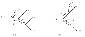
Figure 6: Feynman diagrams of the real emission corrections to top quark decay processes

The Feynman diagrams for NLO real emission corrections to the top quark decay process are shown in Fig. 6. Denoting the helicity amplitude as $\mathcal{M}_{DEC}(\lambda_{t})$, then

$$\mathcal{M}_{DEC}(+) = 2\,\omega_{-}^{t}\frac{\left<\hat{b}\!-\!|\hat{\nu}+\right>\left<\hat{e}\!+\!|\not{\!p}_{-}\not{\!\varepsilon^{*}}_{+}|t+\right>}{p^{2}-m_{t}^{2}}+2\,m_{t}\,\omega_{+}^{t}\frac{\left<\hat{b}\!-\!|\hat{\nu}+\right>\left<\hat{e}\!\!+\!|\!\not{\!\varepsilon^{*}}_{-}|\hat{t}+\right>}{p^{2}-m_{t}^{2}}$$ (73)

$$+ 2\,\omega_{-}^{t}\frac{\left<\hat{e}\!+\!|\hat{t}+\right>\left<\hat{b}\!-\!|\not{\!\varepsilon^{*}}_{+}\not{\!q}_{-}|\hat{\nu}+\right>}{q^{2}},$$

$$\mathcal{M}_{DEC}(-) = 2\,\omega_{+}^{t}\frac{\left<\hat{b}\!-\!|\hat{\nu}+\right>\left<\hat{e}\!\!+\!|\not{\!p}_{-}\not{\!\varepsilon^{*}}_{+}|\hat{t}-\right>}{p^{2}-m_{t}^{2}}+2\,m_{t}\,\omega_{-}^{t}\frac{\left<\hat{b}\!-\!|\hat{\nu}+\right>\left<\!\,\hat{e}\!+\!|\not{\!\varepsilon^{*}}_{-}|\hat{t}-\right>}{p^{2}-m_{t}^{2}}$$ (74)

$$+ 2\,\omega_{+}^{t}\frac{\left<\hat{e}\!+\!|\hat{t}-\right>\left<\hat{b}\!-\!|\not{\!\varepsilon^{*}}_{+}\not{\!q}_{-}|\hat{\nu}+\right>}{q^{2}},$$

with $p=p_{t}-p_{g}$ and $q=p_{b}+p_{g}$. We again suppressed the common factor $\sqrt{2E_{e}}\sqrt{2E_{\nu}}\sqrt{2E_{b}}$, the coupling constants ${\displaystyle g_{s}\left(\frac{g}{\sqrt{2}}\right)^{2}}$, and the $W$ boson propagator ${\displaystyle\frac{1}{p_{W}^{2}-m_{W}^{2}+im_{W}\Gamma_{W}}}$ with $p_{W}=p_{e^{+}}+p_{\nu}$.

V NLO SCV form factors of the single top quark production and decay processes

In this section the analytical results of the effective form factors are given in details together with the corresponding phase space boundary conditions which slice the phase space of real emission corrections into unresolved and resolved regions. Provided with such phase space boundary conditions, one can use the helicity amplitudes given in the previous section to perform numerical calculations. Since the unresolved regions of massless partons differ from the ones of massive partons, we separately consider the massless and massive partons and present the detailed derivations of the SCV form factors in Sec. V.1 and Sec. V.2, respectively. For comparison, we present our results in both the DREG and DRED schemes. We note that the form factors and the crossing functions should be applied consistently in any given scheme.

V.1 NLO corrections to INIT

Let us first examine the initial state corrections to the s-channel single top quark process, cf. Fig. 3. After calculating the effective matrix element with all the partons in the final state, we cross the relevant partons into the initial state to obtain the needed matrix element. In dimension $d=4-2\epsilon$, the NLO matrix element for the vertex $q-\bar{q}^{\prime}-W^{*}$ can be written as

$$M_{\mu}^{q\bar{q}^{\prime}\rightarrow W^{*}} = \frac{ig}{\sqrt{2}}\bar{v}(\bar{q}^{\prime})[f_{1}^{q\bar{q}^{\prime}\rightarrow W^{*}}\gamma_{\mu}]P_{L}u(q),$$ (75)

where $u(q)$($\bar{v}(\bar{q}^{\prime}))$ is the wave function of $q(\bar{q}^{\prime})$, $P_{L}=(1-\gamma_{5})/2$. The calculation of the virtual corrections for the vertex $q-\bar{q}^{\prime}-W^{*}$ is straightforward and after renormalization it yields

$$f_{1}^{q\bar{q}^{\prime}\rightarrow W({\rm virt})} = \frac{\alpha_{s}}{4\pi}C_{F}C_{\epsilon}\left\{-\frac{2}{\epsilon^{2}}+\frac{2}{\epsilon}\ln\frac{\hat{s}}{m_{t}^{2}}-\frac{3}{\epsilon}\right.$$ (76)

$$\left.+\frac{4\pi^{2}}{3}+3\ln\frac{\hat{s}}{m_{t}^{2}}-\ln^{2}\frac{\hat{s}}{m_{t}^{2}}+I_{{\rm scheme}}^{q\bar{q}^{\prime}\rightarrow W({\rm virt})}\right\},$$

where $\hat{s}=2p_{q}\cdot p_{\bar{q}^{\prime}}$, $C_{F}=4/3$, ${\displaystyle C_{\epsilon}=\left(\frac{4\pi\mu^{2}}{m_{t}^{2}}\right)^{\epsilon}\Gamma(1+\epsilon)}$, and the scheme dependent term $I_{\,{\rm scheme}}^{\,q\bar{q}^{\prime}\rightarrow W({\rm virt})}$ is

$$I_{{\rm\,Scheme}}^{\,q\bar{q}^{\prime}\rightarrow W({\rm virt})}=\begin{cases}-8&{\rm in\leavevmode\nobreak\ DREG\leavevmode\nobreak\ scheme},\\ -7&{\rm in\leavevmode\nobreak\ DRED\leavevmode\nobreak\ scheme}.\end{cases}$$ (77)

We have neglected all the possible imaginary parts in the above result and also in what follows, because they do not contribute to cross sections up to the NLO. Note that the tree level amplitude corresponds to setting $f_{1}^{q\bar{q}^{\prime}\rightarrow W}=1$ in Eq. (75).

In the phase space slicing method, the soft and collinear singularities in the virtual corrections, the poles of $\epsilon$ in Eq. (76), should be canceled by the unresolved real emission corrections from processes shown in Eqs. (19)-(21). Below, we will partition the phase space of the real emission corrections to calculate the unresolved contribution.

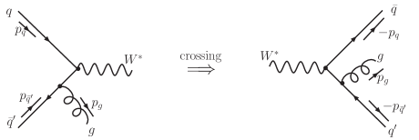
Figure 7: Illustration for crossing the initial state partons into the final state in the process $q\bar{q}^{\prime}\rightarrow W^{*}g$.

As an example, let us examine the $q\bar{q}\rightarrow W^{*}g$ process. After crossing all the initial state partons of the process $q\bar{q}^{\prime}\rightarrow W^{*}g$ into the final state, the particles’ momenta are assigned as in Fig. 7 which implies the crossed process $W^{*}\rightarrow\bar{q}q^{\prime}g$. Let us consider the whole phase space of the process $W^{*}\rightarrow\bar{q}q^{\prime}g$ as the identity and partition it into three regions as shown in Fig. 8:

$$1 \equiv \Theta(\left|s_{\bar{q}g}\right|+\left|s_{q^{\prime}g}\right|-2s_{min})+\Theta(2s_{min}-\left|s_{\bar{q}g}\right|-\left|s_{q^{\prime}g}\right|)$$ (78)

$$- \Theta(\left|s_{\bar{q}g}\right|-2s_{min})\Theta(s_{min}-\left|s_{q^{\prime}g}\right|)-\Theta(\left|s_{q^{\prime}g}\right|-2s_{min})\Theta(s_{min}-\left|s_{\bar{q}g}\right|)$$

$$+ \Theta(\left|s_{\bar{q}g}\right|-2s_{min})\Theta(s_{min}-\left|s_{q^{\prime}g}\right|)+\Theta(\left|s_{q^{\prime}g}\right|-2s_{min})\Theta(s_{min}-\left|s_{\bar{q}g}\right|)$$

$$= \mathcal{F}_{1}+\mathcal{F}_{2}+\mathcal{F}_{3},$$

where

$$\mathcal{F}_{1} = \Theta(\left|s_{\bar{q}g}\right|+\left|s_{q^{\prime}g}\right|-2s_{min})$$ (79)

$$-\Theta(\left|s_{\bar{q}g}\right|-2s_{min})\Theta(s_{min}-\left|s_{q^{\prime}g}\right|)-\Theta(\left|s_{q^{\prime}g}\right|-2s_{min})\Theta(s_{min}-\left|s_{\bar{q}g}\right|),$$

$$\mathcal{F}_{2} = \Theta(2s_{min}-\left|s_{\bar{q}g}\right|-\left|s_{q^{\prime}g}\right|),$$ (80)

$$\mathcal{F}_{3} = \Theta(\left|s_{\bar{q}g}\right|-2s_{min})\Theta(s_{min}-\left|s_{q^{\prime}g}\right|)+\Theta(\left|s_{q^{\prime}g}\right|-2s_{min})\Theta(s_{min}-\left|s_{\bar{q}g}\right|).$$ (81)

Here $\Theta$ is the Heaviside step function and $s_{ij}=2p_{i}\cdot p_{j}$, where $p_{i}$ is the four-momentum of the particle $i$. In the phase space region constrained by function $\mathcal{F}_{1}$ (resolved), there is no soft and collinear divergencies, therefore it can be calculated in four dimensions numerically. The soft region is defined by the function $\mathcal{F}_{2}$, which have both the soft and collinear divergencies. The collinear regions is defined by the function $\mathcal{F}_{3}$ as shown in Fig. 8 which only have the collinear singularities but no soft singularities. In function $\mathcal{F}_{3}$, the first term denotes the collinear region of $g\parallel q^{\prime}$ and the second term represents the collinear region of $g\parallel\bar{q}$.

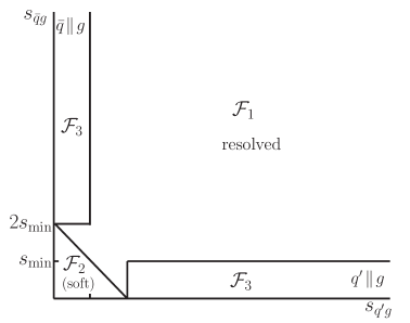
Figure 8: The $s_{\bar{q}g}-s_{q^{\prime}g}$ plane for quark pair annihilation to virtual $W$-boson showing the delineation into soft ($\mathcal{F}_{2}$), collinear ($\mathcal{F}_{2}$) and resolved region ($\ \mathcal{F}_{1}$).

Under the soft approximation, i.e. in the soft region ($\mathcal{F}_{2}$), the squared matrix element can be written as a factor multiplying the squared Born matrix element:

$$\Theta(2s_{min}-\left|s_{\bar{q}g}\right|-\left|s_{q^{\prime}g}\right|)\left|\mathcal{M}(W^{*}\rightarrow\bar{q}q^{\prime}g)\right|^{2}\xrightarrow{p_{g}\rightarrow 0}\hat{f}_{s}^{W^{*}\rightarrow\bar{q}q^{\prime}g}\left|\mathcal{M}(W^{*}\rightarrow\bar{q}q^{\prime})\right|^{2},$$ (82)

where we have defined the eikonal factor $\hat{f}_{s}^{W^{*}\rightarrow\bar{q}q^{\prime}g}$ as

$$\hat{f}_{s}^{W^{*}\rightarrow\bar{q}q^{\prime}g}=g_{s}C_{F}\mu^{2\epsilon}\frac{4(2p_{\bar{q}}\cdot p_{q^{\prime}})}{(2p_{\bar{q}}\cdot p_{g})(2p_{q^{\prime}}\cdot p_{g})}.$$ (83)

It is very simple to analytically integrate the eikonal factors $\hat{f}_{s}^{W^{*}\rightarrow\bar{q}q^{\prime}g}$ in $d$ dimensions over the soft gluon momentum Brandenburg:1997pu and get the soft factor

$$I_{{\rm soft}}^{W^{*}\rightarrow\bar{q}q^{\prime}g} = \frac{g_{s}^{2}}{16\pi^{2}}\frac{C_{F}}{\Gamma(1-\epsilon)}\left(\frac{4\pi\mu_{d}^{2}}{s_{min}}\right)^{2}\left\{\frac{2}{\epsilon^{2}}-\frac{4\ln 2}{\epsilon}-\frac{2}{\epsilon}\ln\left(\frac{s_{min}}{\hat{s}}\right)\right.$$ (84)

$$\left.+4\ln^{2}2-\frac{\pi^{2}}{3}+\ln^{2}\left(\frac{s_{min}}{\hat{s}}\right)+4\ln 2\,\ln\left(\frac{s_{min}}{\hat{s}}\right)\right\}.$$

In addition to being singular in the soft gluon region, the matrix elements are also singular in the collinear region ($\mathcal{F}_{3}$) where the matrix elements exhibit an overall factorization. In the limit $g\parallel\bar{q}$, we define

$$p_{g}\xrightarrow{g\parallel\bar{q}}\xi p_{h},\qquad p_{\bar{q}}\xrightarrow{g\parallel\bar{q}}(1-\xi)p_{h},$$ (85)

with $p_{h}=p_{g}+p_{\bar{q}}.$ In this limit,

$$\Theta(\left|s_{q^{\prime}g}\right|-2s_{min})\Theta(s_{min}-\left|s_{\bar{q}g}\right|)\left|\mathcal{M}(W^{*}\rightarrow\bar{q}q^{\prime}g)\right|^{2}\xrightarrow{g\parallel\bar{q}}\hat{c}^{\bar{q}g\rightarrow\bar{q}}\left|\mathcal{M}(W^{*}\rightarrow\bar{q}q^{\prime})\right|^{2},$$ (86)

where the collinear factor $\hat{c}^{\bar{q}g\rightarrow\bar{q}}$ is defined as Brandenburg:1997pu

$$\hat{c}^{\bar{q}g\rightarrow\bar{q}}=g_{s}^{2}\mu^{2\epsilon}C_{F}\frac{P^{\bar{q}g\rightarrow\bar{q}}(\xi)}{2p_{g}\cdot p_{\bar{q}}}.$$ (87)

The function $P^{\bar{q}g\rightarrow\bar{q}}$ is related to the Altarelli-Parisi splitting function, which depends on the regularization scheme. In this paper, we adopt two schemes: the conventional dimensional regularization (DREG) scheme and the dimensional reduction (DRED) scheme. We have

$$P^{\bar{q}g\rightarrow\bar{q}}(\xi)=\begin{cases}2\,{\displaystyle\frac{1+\xi^{2}-\epsilon(1-\xi)^{2}}{1-\xi},}&{\rm in\leavevmode\nobreak\ DREG\leavevmode\nobreak\ scheme},\\ 2\,{\displaystyle\frac{1+\xi^{2}}{1-\xi},}&{\rm in\leavevmode\nobreak\ DRED\leavevmode\nobreak\ scheme}.\end{cases}$$ (88)

After integrating over the collinear phase space Brandenburg:1997pu for the case $g\parallel q^{\prime}$, we obtain the collinear factor

$$I_{{\rm col}}^{W^{*}\rightarrow\bar{q}q^{\prime}g} = \frac{g_{s}^{2}}{16\pi^{2}}\frac{C_{F}}{\Gamma(1-\epsilon)}\left(\frac{4\pi\mu_{d}^{2}}{s_{min}}\right)^{\epsilon}$$ (89)

$$\times \left\{\frac{4}{\epsilon}\ln\left(\frac{2s_{min}}{\hat{s}}\right)+\frac{3}{\epsilon}-\frac{2\pi^{2}}{3}-2\ln^{2}\left(\frac{2s_{min}}{\hat{s}}\right)+I_{{\rm Scheme}}^{W^{*}\rightarrow\bar{q}q^{\prime}({\rm col})}\right\},$$

where the scheme dependent factor $I_{{\rm Scheme}}^{W^{*}\rightarrow\bar{q}q^{\prime}({\rm col})}$ is

$$I_{{\rm Scheme}}^{W^{*}\rightarrow\bar{q}q^{\prime}({\rm col})}=\begin{cases}7&{\rm in\leavevmode\nobreak\ DREG\leavevmode\nobreak\ scheme},\\ 6&{\rm in\leavevmode\nobreak\ DRED\leavevmode\nobreak\ scheme}.\end{cases}$$ (90)

Summing over the soft and collinear factors and crossing the needed partons into the initial state, we get the contributions to $\mathcal{M}^{q\bar{q}^{\prime}\rightarrow W^{*}}$ from the unresolved real (soft+collinear) corrections from processes (19)-(21) as following:

$$f_{1}^{q\bar{q}^{\prime}\rightarrow W({\rm real})} = \frac{\alpha_{s}}{4\pi}C_{F}C_{\epsilon}\left(\frac{2}{\epsilon^{2}}-\frac{2}{\epsilon}\ln\frac{\hat{s}}{m_{t}^{2}}+\frac{3}{\epsilon}-\frac{4\pi^{2}}{3}+2\ln^{2}2\right.$$ (91)

$$\left.+3\ln\frac{m_{t}^{2}}{s_{min}}-2\ln^{2}\frac{\hat{s}}{s_{min}}+\ln^{2}\frac{\hat{s}}{m_{t}^{2}}+I_{{\rm Scheme}}^{q\bar{q}^{\prime}\rightarrow W({\rm real})}\right),$$

where the scheme dependent term $I_{{\rm\,Scheme}}^{\,q\bar{q}^{\prime}\rightarrow W({\rm real})}$ is

$$I_{{\rm\,Scheme}}^{\,q\bar{q}^{\prime}\rightarrow W({\rm real})}=\begin{cases}7&{\rm in\leavevmode\nobreak\ DREG\leavevmode\nobreak\ scheme},\\ 6&{\rm in\leavevmode\nobreak\ DRED\leavevmode\nobreak\ scheme}.\end{cases}$$ (92)

It is clear that the divergencies of $f_{1}^{q\bar{q}^{\prime}\rightarrow W({\rm virt})}$ and $f_{1}^{q\bar{q}^{\prime}\rightarrow W({\rm real})}$ cancel with each other and the sum is finite and $s_{min}$ dependent. The remaining unresolved real corrections for $q\bar{q}^{\prime}\rightarrow W^{*}$ are included through the process independent, but $s_{min}$ and factorization scheme dependent universal crossing functions.

The corrections from the resolved regions of processes (19)-(21) can be obtained by multiplying the following phase space slicing functions to the corresponding phase space elements and matrix element squares in the cross section calculations:

$$\biggl{[}\Theta(\left|s_{gq}\right|+\left|s_{g\bar{q^{\prime}}}\right|-2s_{min})-\Theta(\left|s_{gq}\right|-2s_{min})\Theta(s_{min}-\left|s_{g\bar{q^{\prime}}}\right|)$$

$$\,\,\,\,\,\,\,\,\,\,\,\,\,\,\,\,\,\,\,\,\,\,\,\,\,\,\,\,\,\,-\Theta(\left|s_{g\bar{q^{\prime}}}\right|-2s_{min})\Theta(s_{min}-\left|s_{gq}\right|)\biggr{]}\leavevmode\nobreak\ \leavevmode\nobreak\ \,\,\,\,{\textrm{for }}\leavevmode\nobreak\ \leavevmode\nobreak\ q\bar{q}^{\prime}\rightarrow W^{*}g\rightarrow t\bar{b}g,\leavevmode\nobreak\ \leavevmode\nobreak\ \leavevmode\nobreak\ \leavevmode\nobreak\$$ (93)

$$\biggl{[}1-\Theta(s_{min}-\left|s_{gq^{\prime}}\right|)\biggr{]}\,\,\,\,\,\,\,\,\,\,\,\,\,\,\,\,\,\,\,\,\,\,\,\,\,\,\,\,\,\,\,\,\,\,\,\,\,\,\,\,\,\,\,\,\,\,\,\,\,\,\,\,\,\,\,\,\,\,\,\,\,\,\,\,\,\,\,\leavevmode\nobreak\ \leavevmode\nobreak\ {\textrm{for }}\leavevmode\nobreak\ \leavevmode\nobreak\ qg\rightarrow W^{*}q^{\prime}\rightarrow t\bar{b}q^{\prime},\leavevmode\nobreak\ \leavevmode\nobreak\ \leavevmode\nobreak\ \leavevmode\nobreak\$$ (94)

$$\biggl{[}1-\Theta(s_{min}-\left|s_{g\bar{q}}\right|)\biggr{]}\,\,\,\,\,\,\,\,\,\,\,\,\,\,\,\,\,\,\,\,\,\,\,\,\,\,\,\,\,\,\,\,\,\,\,\,\,\,\,\,\,\,\,\,\,\,\,\,\,\,\>\,\,\,\,\,\,\,\,\,\,\,\,\,\,\,\,\,\leavevmode\nobreak\ \leavevmode\nobreak\ {\textrm{for }}\leavevmode\nobreak\ \leavevmode\nobreak\ g\bar{q}^{\prime}\rightarrow W^{*}\bar{q}\rightarrow t\bar{b}\bar{q}.$$ (95)

The $\Theta$ functions ensure the amplitude squares to be finite in four dimensions. Therefore, they can be calculated numerically.

V.2 NLO corrections to FINAL

Now we examine the final state corrections to $W_{\mu}^{*}-t-\bar{b}$. The NLO matrix element for the $W^{*}-t-b$ vertex can be written as

$$\mathcal{M}_{\mu}^{W^{*}\rightarrow t\bar{b}} = \frac{ig}{\sqrt{2}}\bar{u}(t)[f_{1}^{W^{*}\rightarrow t\bar{b}}\gamma_{\mu}-f_{2}^{W^{*}\rightarrow t\bar{b}}\frac{(p_{t}-p_{\bar{b}})_{\mu}}{m_{t}}]P_{L}v(\bar{b}).$$ (96)

The above formula is valid only when $W$ boson is on-shell or off-shell but coupled to massless quarks because we have neglected the term proportional to $(p_{t}+p_{\bar{b}})_{\mu}$. At the tree level, $f_{1}^{W\rightarrow t\bar{b}}=1$ and $f_{2}^{W\rightarrow t\bar{b}}=0$. At the NLO, the virtual corrections to $f_{1}^{W\rightarrow t\bar{b}}$ and $f_{2}^{W\rightarrow t\bar{b}}$ are, respectively,

$$f_{1}^{W\rightarrow t\bar{b}({\rm virt})} = \frac{\alpha_{s}}{4\pi}C_{F}C_{\epsilon}\left\{-\frac{1}{\epsilon^{2}}-\frac{5}{2\epsilon}+\frac{2}{\epsilon}\ln\frac{\hat{s}_{1}}{m_{t}^{2}}+\pi^{2}+2{\textrm{Li}}_{2}(\frac{\hat{s}}{\hat{s}_{1}})\right.$$ (97)

$$\left.+3\ln\frac{\hat{s}_{1}}{m_{t}^{2}}-\frac{m_{t}^{2}}{\hat{s}}\ln\frac{\hat{s}_{1}}{m_{t}^{2}}-\ln^{2}\frac{\hat{s}_{1}}{m_{t}^{2}}+I_{\,{\rm Scheme}}^{\,W\rightarrow t\bar{b}({\rm virt})}\right\},$$

$$f_{2}^{W\rightarrow t\bar{b}({\rm virt})} = \frac{\alpha_{s}}{4\pi}C_{F}C_{\epsilon}\left\{\frac{m_{t}^{2}}{\hat{s}}\ln\frac{\hat{s}_{1}}{m_{t}^{2}}\right\},$$ (98)

where $\hat{s}=(p_{t}+p_{\bar{b}})^{2}$, $\hat{s}_{1}=2p_{t}\cdot p_{\bar{b}}=\hat{s}-m_{t}^{2}$ and the scheme dependent term $I_{\,{\rm Scheme}}^{\,W\rightarrow t\bar{b}({\rm virt})}$ is

$$I_{{\rm\,Scheme}}^{\,W\rightarrow t\bar{b}({\rm virt})}=\begin{cases}-6&{\rm in\leavevmode\nobreak\ DREG\leavevmode\nobreak\ scheme,}\\ -5&{\rm in\leavevmode\nobreak\ DRED\leavevmode\nobreak\ scheme.}\end{cases}$$ (99)

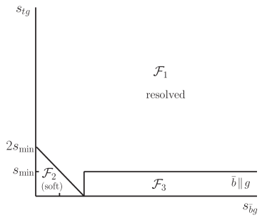
Figure 9: The $s_{tg}-s_{\bar{b}g}$ plane for quark pair annihilation to virtual $W$-boson showing the delineation into soft ($\mathcal{F}_{2}$), collinear ($\mathcal{F}_{2}$) and resolved region ($\mathcal{F}_{1}$).

In the presence of massive top quark, the structure of collinear and soft poles of FINAL matrix elements is completely different from the massless case (INIT). The top quark mass serves as a regularizer for collinear singularities. Thus, the matrix element contain fewer singular structures. However, the presence of the top quark mass leads to more complicated phase space integrals. Again, let us consider the whole phase space of the process $W^{*}\rightarrow t\bar{b}g$ as the identity and partition it into three regions as shown in Fig. 9:

$$1 \equiv \Theta(s_{tg}+s_{\bar{b}g}-2s_{min})+\Theta(2s_{min}-s_{tg}-s_{\bar{b}g})$$ (100)

$$+ \Theta(s_{tg}-2s_{min})\Theta(s_{min}-s_{\bar{b}g})-\Theta(s_{tg}-2s_{min})\Theta(s_{min}-s_{\bar{b}g})$$

$$= \mathcal{F}_{1}+\mathcal{F}_{2}+\mathcal{F}_{3},$$

where

$$\mathcal{F}_{1} = \Theta(s_{tg}+s_{\bar{b}g}-2s_{min})-\Theta(s_{tg}-2s_{min})\Theta(s_{min}-s_{\bar{b}g}),$$ (101)

$$\mathcal{F}_{2} = \Theta(2s_{min}-s_{tg}-s_{\bar{b}g}),$$ (102)

$$\mathcal{F}_{3} = \Theta(s_{tg}-2s_{min})\Theta(s_{min}-s_{\bar{b}g}).$$ (103)

Here again, we divide the phase space of process $W^{*}\rightarrow t\bar{b}g$ into three parts: the resolved region ($\mathcal{F}_{1}$), the soft region ($\mathcal{F}_{2}$) and the collinear region ($\mathcal{F}_{3}$). Moreover, the phase space boundary conditions are much simpler than the case of massless partons, cf. Eqs. (79)-(81).

Under the soft approximation, in the soft region ($\mathcal{F}_{2}$), the squared matrix element can be written as a factor multiplying the squared Born matrix element:

$$\Theta(2s_{min}-s_{tg}-s_{\bar{b}g})\left|\mathcal{M}(W^{*}\rightarrow t\bar{b}g)\right|^{2}\xrightarrow{p_{g}\rightarrow 0}\hat{f}_{s}^{W^{*}\rightarrow tbg}\left|\mathcal{M}(W^{*}\rightarrow t\bar{b})\right|^{2},$$ (104)

where we have defined the eikonal factor $\hat{f}_{s}^{W^{*}\rightarrow t\bar{b}g}$ as Brandenburg:1997pu :

$$\hat{f}_{s}^{W^{*}\rightarrow t\bar{b}g}=g_{s}C_{F}\mu^{2\epsilon}\left[\frac{4(2p_{t}\cdot p_{\bar{b}})}{(2p_{t}\cdot p_{g})(2p_{\bar{b}}\cdot p_{g})}-\frac{4m_{t}^{2}}{(2p_{t}\cdot p_{g})^{2}}\right].$$ (105)

Integrating the eikonal factors $\hat{f}_{s}^{W^{*}\rightarrow t\bar{b}g}$ in $d$ dimensions over the soft gluon momentum Brandenburg:1997pu , we get the soft factor

$$I_{{\rm soft}}^{W^{*}\rightarrow t\bar{b}g} = \frac{g_{s}^{2}}{16\pi^{2}}\frac{C_{F}}{\Gamma(1-\epsilon)}\left(\frac{4\pi\mu_{d}^{2}}{s_{min}}\right)^{2}\left(\frac{s_{min}}{\hat{s}_{1}+m_{t}^{2}}\right)^{-\epsilon}$$ (106)

$$\times \left\{\frac{1}{\epsilon^{2}}--\frac{1}{\epsilon}\left[\ln\left(1+\frac{\hat{s}_{1}}{m_{t}^{2}}\right)+2\ln 2-1\right]\right.$$

$$-\frac{\pi^{2}}{6}+2\ln^{2}2-2\ln 2+\left[2\ln 2+\frac{\hat{s}_{1}+2m_{t}^{2}}{\hat{s}_{1}}\right]\ln\left(1+\frac{\hat{s}_{1}}{m_{t}^{2}}\right)$$

$$\left.-\frac{1}{2}\ln^{2}\left(1+\frac{\hat{s}_{1}}{m_{t}^{2}}\right)-2{\rm Li_{2}\left(\frac{\hat{s}_{1}}{\hat{s}_{1}+m_{t}^{2}}\right)}\right\}.$$

In the collinear region ($\mathcal{F}_{3}$), where $g\parallel\bar{b}$, the matrix elements exhibit an overall factorization as

$$\Theta(s_{tg}-2s_{min})\Theta(s_{min}-s_{\bar{b}g})\left|\mathcal{M}(W^{*}\rightarrow t\bar{b}g)\right|^{2}\xrightarrow{g\parallel\bar{b}}\hat{c}^{\bar{b}g\rightarrow\bar{b}}(\xi)\left|\mathcal{M}(W^{*}\rightarrow t\bar{b})\right|^{2},$$ (107)

where the collinear factor $\hat{c}^{\bar{b}g\rightarrow\bar{b}}$ is defined as Brandenburg:1997pu :

$$\hat{c}^{\bar{b}g\rightarrow\bar{b}}=g_{s}^{2}\mu^{2\epsilon}C_{F}\left[\frac{P^{\bar{b}g\rightarrow\bar{b}}(\xi)}{2p_{\bar{b}}\cdot p_{g}}-\frac{4m_{t}^{2}}{\left(2p_{t}\cdot p_{g}\right)^{2}}\right],$$ (108)

in which $P^{\bar{b}g\rightarrow\bar{b}}(\xi)$ is same as Eq. (88). Integrating over the collinear phase space Brandenburg:1997pu , we get the collinear factor

$$I_{{\rm col}}^{W^{*}\rightarrow t\bar{b}g} = \frac{g_{s}^{2}}{16\pi^{2}}\frac{C_{F}}{\Gamma(1-\epsilon)}\left(\frac{4\pi\mu_{d}^{2}}{s_{min}}\right)^{\epsilon}$$ (109)

$$\times \left\{\frac{2}{\epsilon}\left[\ln^{2}\left(\frac{2s_{min}}{\hat{s}}\right)+\frac{3}{4}\right]-\frac{\pi^{2}}{3}-\ln^{2}\left(\frac{2s_{min}}{\hat{s}}\right)-\frac{m_{t}^{2}}{\hat{s}_{1}}+I_{{\rm Scheme}}^{W^{*}\rightarrow t\bar{b}g({\rm col})}\right\},$$

where the scheme dependent factor $I_{{\rm Scheme}}^{W^{*}\rightarrow t\bar{b}g({\rm col})}$ is

$$I_{{\rm Scheme}}^{W^{*}\rightarrow t\bar{b}g({\rm col})}=\begin{cases}{\displaystyle\frac{7}{2}}&{\rm in\leavevmode\nobreak\ DREG\leavevmode\nobreak\ scheme},\\ 3&{\rm in\leavevmode\nobreak\ DRED\leavevmode\nobreak\ scheme}.\end{cases}$$ (110)

Summing over the soft and collinear factor, we get the contributions to $\mathcal{M}^{W^{*}\rightarrow t\bar{b}}$ from the unresolved real (soft+collinear) corrections as following:

$$f_{1}^{W^{*}\rightarrow t\bar{b}g({\rm real})} = \frac{\alpha_{s}}{4\pi}C_{F}C_{\epsilon}\left\{\frac{1}{\epsilon^{2}}+\frac{5}{2\epsilon}-\frac{2}{\epsilon}\ln\frac{\hat{s}_{1}}{m_{t}^{2}}-\frac{2\pi^{2}}{3}+\ln^{2}2-2\ln 2\right.$$ (111)

$$-2{\textrm{Li}}_{2}(\frac{\hat{s}_{1}}{\hat{s}})-\frac{7}{2}\ln\frac{s_{min}}{m_{t}^{2}}+2\ln 2\ln\frac{\hat{s}_{1}}{m_{t}^{2}}+(2+\frac{2m_{t}^{2}}{\hat{s}_{1}})\ln\frac{\hat{s}}{m_{t}^{2}}$$

$$\left.-\ln^{2}\frac{\hat{s}}{m_{t}^{2}}-\ln^{2}\frac{\hat{s}_{1}}{s_{min}}+2\ln\frac{\hat{s}_{1}}{m_{t}^{2}}\ln\frac{s_{min}}{m_{t}^{2}}-\frac{m_{t}^{2}}{\hat{s}_{1}}+I_{\,{\rm Scheme}}^{\,W^{*}\rightarrow t\bar{b}g({\rm real})}\right\},$$

where the scheme dependent term $I_{{\rm\,Scheme}}^{\,W^{*}\rightarrow t\bar{b}g({\rm real})}$ is

$$I_{\,{\rm Scheme}}^{\,W^{*}\rightarrow t\bar{b}g({\rm real})}=\begin{cases}{\displaystyle\frac{7}{2}}&{\rm in\leavevmode\nobreak\ DREG\leavevmode\nobreak\ scheme},\\ 3&{\rm in\leavevmode\nobreak\ DRED\leavevmode\nobreak\ scheme}.\end{cases}$$ (112)

The correction from the resolved regions of process (22) can be obtained by multiplying the following phase space slicing functions to the corresponding phase space elements and matrix element squares in the cross section calculations:

$$\biggl{[}\Theta(s_{tg}+s_{\bar{b}g}-2s_{min})-\Theta(s_{tg}-2s_{min})\Theta(s_{min}-s_{\bar{b}g})\biggr{]}.$$ (113)

V.3 NLO corrections to LIGHT

The NLO matrix element for the $q-W^{*}_{\mu}-q^{\prime}$ vertex can be written as

$$M_{\mu}^{q\rightarrow W^{*}q^{\prime}} = \frac{ig}{\sqrt{2}}\bar{u}(q^{\prime})[f_{1}^{q\rightarrow W^{*}q^{\prime}}\gamma_{\mu}P_{L}]u(q),$$ (114)

where $u(q)$($\bar{u}(q^{\prime}))$ is the wave function of $q(q^{\prime})$. The virtual correction to $f_{1}^{q\rightarrow W^{*}q^{\prime}}$ is

$$f_{1}^{q\rightarrow W^{*}q^{\prime}({\rm virt})} = \frac{\alpha_{s}}{4\pi}C_{F}C_{\epsilon}\left\{-\frac{2}{\epsilon^{2}}+\frac{2}{\epsilon}\ln(\frac{-\hat{t}}{m_{t}^{2}})-\frac{3}{\epsilon}\right.$$ (115)

$$\left.\,\,\,\,\,\,\,\,\,\,\,\,\,\,\,\,\,\,\,\,\,\,\,\,+\frac{\pi^{2}}{3}+3\ln(\frac{-\hat{t}}{m_{t}^{2}})-\ln^{2}(\frac{-\hat{t}}{m_{t}^{2}})+I_{\,{\rm scheme}}^{\,q\rightarrow W^{*}q^{\prime}({\rm virt})}\right\},$$

where $\hat{t}=-2p_{q}\cdot p_{q^{\prime}}$ and the scheme dependent term $I_{\,{\rm Scheme}}^{\,q\rightarrow W^{*}q^{\prime}({\rm virt})}$ is

$$I_{\,{\rm Scheme}}^{\,q\rightarrow W^{*}q^{\prime}({\rm virt})}=\begin{cases}-8&{\rm in\leavevmode\nobreak\ DREG\leavevmode\nobreak\ scheme},\\ -7&{\rm in\leavevmode\nobreak\ DRED\leavevmode\nobreak\ scheme}.\end{cases}$$ (116)

The tree level amplitude can be obtained by setting $f_{1}^{q\rightarrow W^{*}q^{\prime}}=1$.

We now consider the unresolved real correction to $f_{1}^{q\rightarrow W^{*}q^{\prime}}$. There are two processes that contribute to $q-W^{*}_{\mu}-q^{\prime}$ vertex:

• $bq\rightarrow tq^{\prime}g\,(I)$, in which the gluon only connects with the light quark ($q$,$q^{\prime}$) line, cf. Eqs. (24) and (25),

• $bg\rightarrow t\bar{q}q^{\prime}$, cf. Eq. (28).

The soft and collinear divergent regions of $bq\rightarrow tq^{\prime}g\,(I)$ can be constrained by the function

$$\biggl{[}\Theta(2s_{min}-\left|s_{qg}\right|-\left|s_{q^{\prime}g}\right|)$$

$$+\Theta(\left|s_{qg}\right|-2s_{min})\Theta(s_{min}-\left|s_{q^{\prime}g}\right|)$$

$$+\Theta(\left|s_{q^{\prime}g}\right|-2s_{min})\Theta(s_{min}-\left|s_{qg}\right|)\biggl{]}.$$ (117)

In the above function, the first term constrains $p_{g}$ to be soft and the second and third terms restrict $p_{g}$ to be collinear with $p_{q^{\prime}}$ and $p_{q}$, respectively. The process $bg\rightarrow t\bar{q}q^{\prime}$ has only collinear divergent phase space region which is projected by

$$\biggl{[}\Theta(s_{min}-\left|s_{\bar{q}g}\right|)+\Theta(s_{min}-\left|s_{q^{\prime}g}\right|)\biggr{]},$$ (118)

in which the two terms require $p_{g}$ to be collinear with $p_{q}$ and $p_{q^{\prime}}$, respectively. After performing all the above constrained phase space integrations analytically, one can get the contribution to $f_{1}^{q\rightarrow W^{*}q^{\prime}}$ from the unresolved real emission corrections as:

$$f_{1}^{q\rightarrow W^{*}q^{\prime}({\rm real})} = \frac{\alpha_{s}}{4\pi}C_{F}C_{\epsilon}\left\{\frac{2}{\epsilon^{2}}-\frac{2}{\epsilon}\ln(\frac{-\hat{t}}{m_{t}^{2}})+\frac{3}{\epsilon}-\frac{4\pi^{2}}{3}+2\ln^{2}2\right.$$ (119)

$$\left.+3\ln\frac{m_{t}^{2}}{s_{min}}-2\ln^{2}(\frac{-\hat{t}}{s_{min}})+\ln^{2}(\frac{-\hat{t}}{m_{t}^{2}})+I_{\,{\rm Scheme}}^{\,q\rightarrow W^{*}q^{\prime}({\rm real})}\right\},$$

where the scheme dependent term $I_{{\rm\,Scheme}}^{\,q\rightarrow W^{*}q^{\prime}({\rm real})}$ is

$$I_{\,{\rm Scheme}}^{\,q\rightarrow W^{*}q^{\prime}({\rm real})}=\begin{cases}7&{\rm in\leavevmode\nobreak\ DREG\leavevmode\nobreak\ scheme},\\ 6&{\rm in\leavevmode\nobreak\ DRED\leavevmode\nobreak\ scheme}.\end{cases}$$ (120)

It is clear that the divergencies of $f_{1}^{q\rightarrow W^{*}q^{\prime}({\rm virt})}$ and $f_{1}^{q\rightarrow W^{*}q^{\prime}({\rm real})}$ cancel with each other and the sum is finite and $s_{min}$ dependent. The remaining unresolved real corrections for $q\rightarrow W^{*}q^{\prime}$ are included through the process independent, but $s_{min}$ and factorization scheme dependent universal crossing functions.

The resolved phase spaces without divergent regions are obtained by multiplying the following function to the phase space:

$$\biggl{[}\Theta(\left|s_{gq}\right|+\left|s_{q^{\prime}g}\right|-2s_{min})-\Theta(\left|s_{gq}\right|-2s_{min})\Theta(s_{min}-\left|s_{q^{\prime}g}\right|)$$

$$\,\,\,\,\,\,\,\,\,\,\,\,\,\,\,\,\,\,\,\,\,\,\,\,\,\,\,\,\,\,-\Theta(\left|s_{q^{\prime}g}\right|-2s_{min})\Theta(s_{min}-\left|s_{gq}\right|)\biggr{]}\,\,\,\,\,\,\,\,\,\,\,\,\,\,\,\,\,\,\,\,{\rm for}\,\,\,\,bq\rightarrow tq^{\prime}g(I),$$ (121)

$$\biggl{[}1-\Theta(s_{min}-\left|s_{q^{\prime}g}\right|)-\Theta(s_{min}-\left|s_{\bar{q}g}\right|)\biggr{]}\,\,\,\,\,\,\,\,\,\,\,\,\,\,\,\,\,\,\,\,\,\,\,\,\,\,\,\,\,\,\,\,\,\,\,\,{\rm for}\,\,\,\,bg\rightarrow t\bar{q}q^{\prime}.$$ (122)

V.4 NLO corrections to HEAVY

The NLO matrix element for the $b-W^{*}_{\mu}-t$ vertex can be written as

$$M_{\mu}^{bW^{*}\rightarrow t} = \frac{ig}{\sqrt{2}}\bar{u}(t)[f_{1}^{bW^{*}\rightarrow t}\gamma_{\mu}-f_{2}^{bW^{*}\rightarrow t}\frac{(p_{b}+p_{t})_{\mu}}{m_{t}}]P_{L}u(b).$$ (123)

The above formula is valid only when $W$ boson is on-shell or off-shell but coupled to massless quarks because we have neglected the term proportional to $(p_{t}-p_{b})_{\mu}$. At the LO, $f_{1}^{bW^{*}\rightarrow t}=1$ and $f_{2}^{bW^{*}\rightarrow t}=0$. At the NLO, the virtual correction to $f_{1}^{bW^{*}\rightarrow t}$ and $f_{2}^{bW^{*}\rightarrow t}$ are

$$f_{1}^{bW^{*}\rightarrow t({\rm virt})} = \frac{\alpha_{s}}{4\pi}C_{F}C_{\epsilon}\left\{-\frac{1}{\epsilon^{2}}-\frac{5}{2\epsilon}+\frac{2}{\epsilon}\ln(\frac{-\hat{t}_{1}}{m_{t}^{2}})+2{\textrm{Li}}_{2}(\frac{\hat{t}}{\hat{t}_{1}})\right.$$ (124)

$$\left.+3\ln(\frac{-\hat{t}_{1}}{m_{t}^{2}})-\frac{m_{t}^{2}}{\hat{t}}\ln(\frac{-\hat{t}_{1}}{m_{t}^{2}})-\ln^{2}(\frac{-\hat{t}_{1}}{m_{t}^{2}})+I_{\,{\rm Scheme}}^{\,bW^{*}\rightarrow t({\rm virt})}\right\},$$

$$f_{2}^{bW^{*}\rightarrow t({\rm virt})} = \frac{\alpha_{s}}{4\pi}C_{F}C_{\epsilon}\left\{\frac{m_{t}^{2}}{\hat{t}}\ln(\frac{-\hat{t}_{1}}{m_{t}^{2}})\right\},$$ (125)

where $\hat{t}_{1}=\hat{t}-m_{t}^{2}=-2p_{b}\cdot p_{t}$, and the scheme dependent term $I_{\,{\rm Scheme}}^{\,bW^{*}\rightarrow t({\rm virt})}$ is

$$I_{\,{\rm Scheme}}^{\,bW^{*}\rightarrow t({\rm virt})}=\begin{cases}-6&{\rm in\leavevmode\nobreak\ DREG\leavevmode\nobreak\ scheme},\\ -5&{\rm in\leavevmode\nobreak\ DRED\leavevmode\nobreak\ scheme}.\end{cases}$$ (126)

We now consider the unresolved real correction to $f_{1}^{bW^{*}\rightarrow t}$. The unresolved real correction to $f_{1}^{bW^{*}\rightarrow t}$ comes from the soft and collinear regions of the following three processes:

• $bq\rightarrow tq^{\prime}g\,(II)$, in which the gluon only connect with the heavy quark ($t$,$b$) line, cf. Eqs. (24) and (25),

• $qg\rightarrow tq^{\prime}\bar{b}$, cf. Eq. (26),

• $\bar{q}^{\prime}g\rightarrow\bar{q}\bar{b}t$, cf. Eq. (27).

The soft and collinear divergent regions of $bq\rightarrow tq^{\prime}g\,(II)$ are sliced out by

$$\biggl{[}\Theta(2s_{min}-\left|s_{bg}\right|-\left|s_{tg}\right|)+\Theta(\left|s_{tg}\right|-2s_{min})\Theta(s_{min}-\left|s_{bg}\right|)\biggr{]}.$$ (127)

The $qg\rightarrow tq^{\prime}\bar{b}$ and $\bar{q}^{\prime}g\rightarrow\bar{q}\bar{b}t$ processes both have the collinear divergent region restricted by $\Theta(s_{min}-\left|s_{\bar{b}g}\right|)$. After integrating out the soft and collinear regions, we get the contribution to the form factor $f_{1}^{bW^{*}\rightarrow t}$ from the unresolved real emission corrections as:

$$f_{1}^{bW^{*}\rightarrow t({\rm real})} = \frac{\alpha_{s}}{4\pi}C_{F}C_{\epsilon}\left\{\frac{1}{\epsilon^{2}}+\frac{5}{2\epsilon}-\frac{2}{\epsilon}\ln\frac{-\hat{t}_{1}}{m_{t}^{2}}-\frac{2\pi^{2}}{3}+\ln^{2}2-2\ln 2-2{\textrm{Li}}_{2}(\frac{-\hat{t}_{1}}{m_{t}^{2}-\hat{t}_{1}})\right.$$ (128)

$$-\frac{7}{2}\ln\frac{s_{min}}{m_{t}^{2}}+2\ln 2\ln(\frac{-\hat{t}_{1}}{m_{t}^{2}})+(2-\frac{2m_{t}^{2}}{\hat{t}_{1}})\ln(1-\frac{\hat{t}_{1}}{m_{t}^{2}})-\ln^{2}(1-\frac{\hat{t}_{1}}{m_{t}^{2}})$$

$$\left.-\ln^{2}(\frac{-\hat{t}_{1}}{m_{t}^{2}})-\ln^{2}\frac{s_{min}}{m_{t}^{2}}+4\ln(\frac{-\hat{t}_{1}}{m_{t}^{2}})\ln\frac{s_{min}}{m_{t}^{2}}+\frac{m_{t}^{2}}{\hat{t}_{1}}+I_{\,{\rm Scheme}}^{\,bW^{*}\rightarrow t({\rm real})}\right\},$$

where the scheme dependent term $I_{\,{\rm Scheme}}^{\,bW^{*}\rightarrow t({\rm real})}$ is

$$I_{\,{\rm Scheme}}^{\,bW^{*}\rightarrow t({\rm real})}=\begin{cases}{\displaystyle\frac{7}{2}}&{\rm in\leavevmode\nobreak\ DREG\leavevmode\nobreak\ scheme},\\ 3&{\rm in\leavevmode\nobreak\ DRED\leavevmode\nobreak\ scheme}.\end{cases}$$ (129)

and the remaining unresolved real corrections for $bW^{*}\rightarrow t$ are included through the process independent, but $s_{min}$ and factorization scheme dependent universal crossing functions.

The resolved phase spaces without divergent regions are obtained by multiplying the following function to the phase space:

$$\biggl{[}\Theta(\left|s_{bg}\right|+\left|s_{tg}\right|-2s_{min})-\Theta(\left|s_{tg}\right|-2s_{min})\Theta(s_{min}-\left|s_{bg}\right|)\biggr{]}\,\,\,\, {\rm for}\,\,\,bq\rightarrow tq^{\prime}g\,(II),$$

$$\biggl{[}1-\Theta(s_{min}-\left|s_{\bar{b}g}\right|)\biggr{]}\,\,\,\,\,\,\,\,\,\,\,\,\,\,\,\,\,\,\,\, {\rm for}\,\,\,qg\rightarrow tq^{\prime}\bar{b}\leavevmode\nobreak\ \rm{and}$$

$$\leavevmode\nobreak\ \leavevmode\nobreak\ \leavevmode\nobreak\ \leavevmode\nobreak\ \leavevmode\nobreak\ \bar{q}^{\prime}g\rightarrow\bar{q}\bar{b}t.$$ (131)

V.5 NLO corrections to the decay process $t\rightarrow Wb^{\prime}$

The NLO matrix element for the $t-W-b^{\prime}$ vertex can be written as

$$M_{\mu}^{t\rightarrow Wb} = \frac{ig}{\sqrt{2}}\bar{u}(b^{\prime})[f_{1}^{t\rightarrow Wb^{\prime}}\gamma_{\mu}P_{L}+f_{2}^{t\rightarrow Wb^{\prime}}\frac{(p_{t}+p_{b^{\prime}})_{\mu}}{m_{t}}P_{R}]u(t),$$ (132)

where $P_{R}=(1+\gamma_{5})/2$ and $b^{\prime}$ denotes the bottom quark from the top decay. At the tree level, $f_{1}^{t\rightarrow Wb^{\prime}}=1$, $f_{2}^{t\rightarrow Wb^{\prime}}=0$. At the NLO, the virtual correction to $f_{1}^{t\rightarrow Wb^{\prime}}$ and $f_{2}^{t\rightarrow Wb^{\prime}}$ are, respectively,

$$f_{1}^{t\rightarrow Wb^{\prime}({\rm virt})} = \frac{\alpha_{s}}{4\pi}C_{F}C_{\epsilon}\left\{-\frac{1}{\epsilon^{2}}-\frac{5}{2\epsilon}+\frac{2}{\epsilon}\ln(1-\beta_{W})+2{\textrm{Li}}_{2}(\frac{\beta_{W}}{\beta_{W}-1})\right.$$ (133)

$$\left.+\frac{3\beta_{W}-1}{\beta_{W}}\ln(1-\beta_{W})-\ln^{2}(1-\beta_{W})+I_{\,{\rm Scheme}}^{\,t\rightarrow Wb^{\prime}({\rm virt})}\right\},$$

$$f_{2}^{t\rightarrow Wb^{\prime}({\rm virt})} = \frac{\alpha_{s}}{4\pi}C_{F}C_{\epsilon}\left\{\frac{1}{\beta_{W}}\ln(1-\beta_{W})\right\},$$ (134)

where $\beta_{W}=m_{W}^{2}/m_{t}^{2}$, and the scheme dependent term $I_{\,{\rm Scheme}}^{\,t\rightarrow Wb^{\prime}({\rm virt})}$ is

$$I_{\,{\rm Scheme}}^{\,t\rightarrow Wb^{\prime}({\rm virt})}=\begin{cases}-6&{\rm in\leavevmode\nobreak\ DREG\leavevmode\nobreak\ scheme},\\ -5&{\rm in\leavevmode\nobreak\ DRED\leavevmode\nobreak\ scheme}.\end{cases}$$ (135)

The unresolved real correction to $f_{1}^{t\rightarrow Wb^{\prime}}$ is obtained by integrating out the soft and collinear regions of $t\rightarrow Wb^{\prime}g$ which are sliced by

$$\biggl{[}\Theta(2s_{min}-\left|s_{tg}\right|-\left|s_{b^{\prime}g}\right|)+\Theta(\left|s_{tg}\right|-2s_{min})\Theta(s_{min}-\left|s_{b^{\prime}g}\right|)\biggr{]}.$$ (136)

After integrating over the sliced regions, we get the contribution to $f_{1}^{t\rightarrow Wb^{\prime}}$ as

$$f_{1}^{t\rightarrow Wb^{\prime}({\rm real})} = \frac{\alpha_{s}}{4\pi}C_{F}C_{\epsilon}\left\{\frac{1}{\epsilon^{2}}+\frac{5}{2\epsilon}-\frac{2}{\epsilon}\ln(1-\beta_{W})-\frac{2\pi^{2}}{3}+\ln^{2}2-2\ln 2\right.$$ (137)

$$-2{\textrm{Li}}_{2}(\frac{1-\beta_{W}}{2-\beta_{W}})-\frac{7}{2}\ln\frac{s_{min}}{m_{t}^{2}}+2\ln 2\ln(1-\beta_{W})$$

$$+\frac{4-2\beta_{W}}{1-\beta_{W}}\ln(2-\beta_{W})-\ln^{2}(2-\beta_{W})-\ln^{2}(1-\beta_{W})$$

$$\left.-\ln^{2}\frac{s_{min}}{m_{t}^{2}}+4\ln(1-\beta_{W})\ln\frac{s_{min}}{m_{t}^{2}}-\frac{1}{1-\beta_{W}}+I_{{\rm\,Scheme}}^{\,t\rightarrow Wb^{\prime}({\rm real})}\right\},$$

where the scheme dependent term $I_{\,{\rm Scheme}}^{\,t\rightarrow Wb^{\prime}({\rm real})}$ is

$$I_{\,{\rm Scheme}}^{\,t\rightarrow Wb^{\prime}({\rm real})}=\begin{cases}{\displaystyle\frac{7}{2}}&{\rm in\leavevmode\nobreak\ DREG\leavevmode\nobreak\ scheme},\\ 3&{\rm in\leavevmode\nobreak\ DRED\leavevmode\nobreak\ scheme}.\end{cases}$$ (138)

The resolved region of $t\rightarrow Wb^{\prime}g$ is obtained by multiplying the following function to the phase space:

$$\biggl{[}\Theta(\left|s_{tg}\right|+\left|s_{b^{\prime}g}\right|-2s_{min})-\Theta(\left|s_{tg}\right|-2s_{min})\Theta(s_{min}-\left|s_{b^{\prime}g}\right|)\biggr{]}.$$ (139)

We have checked the formulas of (132)-(139) by comparing the result of NLO correction to $\Gamma(t\rightarrow Wb^{\prime})$ with Ref. Li:1990qf .

VI Combining the production and decay processes

With those building blocks given in the above sections, the NLO QCD corrections to single top quark production and decay can be computed, keeping the full information on the spin configuration of the intermediate top quark state. The general differential hadronic cross section at NLO can be written as

$$d\sigma(H_{1}H_{2}\rightarrow YX)$$ (140)

$$= \sum\limits_{a,b}\int dx_{1}dx_{2}\Biggl{\{}f_{a}^{H_{1}}(x_{1},\mu_{F})f_{b}^{H_{2}}(x_{2},\mu_{F})\times[d\sigma_{0}(ab\rightarrow Y)+d\sigma_{1}(ab\rightarrow Y)]$$

$$\,\,\,\,\,\,\,\,\,\,\,\,\,\,\,\,\,\,\,\,\,\,\,\,\,\,\,\,\,\,\,\,\,\,\,\,+\alpha_{s}f_{a}^{H_{1}}(x_{1},\mu_{F})C_{b}^{H_{2}}(x_{2},\mu_{F},s_{min})d\sigma_{0}(ab\rightarrow Y)$$

$$\,\,\,\,\,\,\,\,\,\,\,\,\,\,\,\,\,\,\,\,\,\,\,\,\,\,\,\,\,\,\,\,\,\,\,\,+\alpha_{s}C_{a}^{H_{1}}(x_{1},\mu_{F},s_{min})f_{b}^{H_{2}}(x_{2},\mu_{F})d\sigma_{0}(ab\rightarrow Y)+(x_{1}\leftrightarrow x_{2})\Biggr{\}},$$

where $d\sigma_{0}$ is the leading-order subprocess cross section, $d\sigma_{1}$ is the $O(\alpha_{S})$ “crossed” subprocess cross section, cf. Fig. 2.

We now consider the single top quark production subprocess $ab\rightarrow t_{\lambda}h_{1}$ with $t_{\lambda}\rightarrow W_{\rho}h_{2}$ and $W_{\rho}\rightarrow l\nu$. (Here, $h_{1}$ and $h_{2}$ stand for any single parton or multiple partons. $\lambda$ and $\rho$ are the top quark spin and $W$ boson polarization indices, respectively) In the frame work of NWA, the cross section can be written as

$$d\sigma(ab\rightarrow l\nu h_{1}h_{2}) = \frac{1}{2\hat{s}}|\sum\limits_{\lambda,\rho}M(ab\rightarrow t_{\lambda}h_{1})M(t_{\lambda}\rightarrow W_{\rho}h_{2})M(W_{\rho}\rightarrow l\nu)|^{2}$$ (141)

$$\times S_{F}\frac{1}{2m_{t}\Gamma_{t}}\frac{1}{2m_{W}\Gamma_{W}}d\Phi(ab\rightarrow th_{1})d\Phi(t\rightarrow Wh_{2})d\Phi(W\rightarrow\ell\nu),$$

where $S_{F}$ denotes the proper spin and color factors, $d\Phi$’s are the phase space elements (${\displaystyle(2\pi)^{4}\delta^{4}(P-\sum p_{i})\prod\frac{d^{3}\vec{p}_{i}}{2E_{i}(2\pi)^{3}}}$). At the LO, $\Gamma_{t}$ in the above equation should be replaced by the Born level decay width $\Gamma^{0}_{t}(t\rightarrow bW)$. At the NLO, special cares should be taken to assign $\Gamma_{t}$, cf. Eq. (149). $\Gamma_{W}$ is the $W$ boson total decay width.

The matrix element square can be calculated as follows. The sum over $\rho$ (the polarization state of the $W$ boson from top decay) is equivalent to the following replacement in $M(t_{\lambda}\rightarrow W_{\rho}h_{2})$:

$$\varepsilon_{W}^{\mu}\rightarrow\frac{g}{2\sqrt{2}}\bar{u}_{\nu}\gamma^{\mu}(1-\gamma_{5})v_{\ell}.$$ (142)

We denote the result by $M(t_{\lambda}\rightarrow Wh_{2})$. Decomposing $M(ab\rightarrow t_{\lambda}h_{1})$ and $M(t_{\lambda}\rightarrow Wh_{2})$ by

$$M(ab\rightarrow t_{\lambda}h_{1}) = \bar{u}_{\lambda}(p_{t})M^{prd},$$ (143)

$$M(t_{\lambda}\rightarrow Wh_{2}) = M^{dec}u_{\lambda}(p_{t}),$$ (144)

where we have explicitly separated the on-shell top quark spinors from both the production and the decay matrix elements, then we have

$$|\sum\limits_{\lambda,\rho}M(ab\rightarrow t_{\lambda}h_{1})M(t_{\lambda}\rightarrow W_{\rho}h_{2})M(W_{\rho}\rightarrow l\nu)|^{2}=|M^{dec}(\hbox to0.0pt{/\hss}p_{t}+m_{t})M^{prd}|^{2}.$$ (145)

In our calculations, $M^{dec}$ and $M^{prd}$ are calculated numerically using helicity amplitude approach and can be easily obtained from the formulas presented in the sections III and IV. Eqs. (142) and (145) guarantee that the spin and angular correlations of the decay products are preserved.

Denoting

$$d\Phi^{{\rm LO}} = S_{F}\frac{1}{2m_{t}\Gamma_{t}^{0}}\frac{1}{2m_{W}\Gamma_{W}}d\Phi(ab\rightarrow th_{1})d\Phi(t\rightarrow Wh_{2})d\Phi(W\rightarrow\ell\nu),$$ (146)

$$d\Phi^{{\rm NLO}} = S_{F}\frac{1}{2m_{t}\Gamma_{t}}\frac{1}{2m_{W}\Gamma_{W}}d\Phi(ab\rightarrow th_{1})d\Phi(t\rightarrow Wh_{2})d\Phi(W\rightarrow\ell\nu),$$ (147)

where $\Gamma_{t}=\Gamma_{t}^{0}(t\rightarrow bW)+\Gamma_{t}^{1}(t\rightarrow bW)$ and $\Gamma_{t}^{1}(t\rightarrow bW)$ is the $O(\alpha_{S})$ correction to the Born level decay width $\Gamma_{t}^{0}(t\rightarrow bW)$, the LO subprocess cross section is

$$d\sigma_{0}(ab\rightarrow l\nu h_{1}h_{2}) = \frac{1}{2\hat{s}}|M_{0}^{dec}(\hbox to0.0pt{/\hss}p_{t}+m_{t})M_{0}^{prd}|^{2}d\Phi^{{\rm LO}},$$ (148)

where $M_{0}^{prd,dec}$ stand for the LO amplitude. The NLO ”crossed” subprocess cross section is

$$d\sigma_{1}(ab\rightarrow l\nu h_{1}h_{2}) = \frac{1}{2\hat{s}}|M_{0}^{dec}(\hbox to0.0pt{/\hss}p_{t}+m_{t})M_{1R}^{prd}|^{2}d\Phi^{{\rm LO}}$$ (149)

$$+ \frac{1}{2\hat{s}}2{\textrm{Re}}\big{[}M_{0}^{dec}(\hbox to0.0pt{/\hss}p_{t}+m_{t})M_{1SCV}^{prd}(M_{0}^{dec}(\hbox to0.0pt{/\hss}p_{t}+m_{t})M_{0}^{prd})^{\dagger}\big{]}d\Phi^{{\rm LO}}$$

$$+ \frac{1}{2\hat{s}}2{\textrm{Re}}\big{[}M_{1SCV}^{dec}(\hbox to0.0pt{/\hss}p_{t}+m_{t})M_{0}^{prd}(M_{0}^{dec}(\hbox to0.0pt{/\hss}p_{t}+m_{t})M_{0}^{prd})^{\dagger}\big{]}d\Phi^{{\rm NLO}}$$

$$+ \frac{1}{2\hat{s}}|M_{1R}^{dec}(\hbox to0.0pt{/\hss}p_{t}+m_{t})M_{0}^{prd}|^{2}d\Phi^{{\rm NLO}},$$

where $M_{1SCV,1R}^{prd,dec}$ stand for the $O(\alpha_{S})$ amplitudes contributed from either soft+collinear+virtual or resolved real corrections for the production or decay processes. The first term is the real NLO correction from production. The second term is the soft+collinear+virtual correction from production. The last two terms are the corrections from the top quark decay. If no kinematical cut is applied, the last two terms cancel each other, which means there is no net correction to the cross section from the top quark decay. Because the virtual correction processes and the real correction processes have different phase spaces $d\Phi^{{\rm LO}}$ and $d\Phi^{{\rm NLO}}$, we calculate them separately using different Monte Carlo programs.

VII Conclusions

Precision measurement of the single top quark events requires more accurate theoretical prediction. The fully NLO differential cross section for on-shell single top quark production has been calculated two years ago, but NLO corrections to the top quark decay process are not included, nor the effect of the top quark width. Since the top quark production and decay do not occur in isolation from each other, a theoretical study that includes both kinds of corrections and keeps the spin correlations between the final state particles is in order.

In this paper we have presented a complete calculation of NLO QCD corrections to both s-channel and t-channel single top quark production and decay processes at hadron colliders. In our calculation the phase space slicing method with one cutoff scale is adopted because it takes advantage of the generalized crossing property of the NLO matrix elements to reduce the analytical calculations. After calculating the effective form factors with all the partons in the final state, we can easily cross the needed partons into the initial state to calculate the s-channel or t-channel single top quark cross sections. To respect the spin correlations between the final state particles, all the amplitudes are calculated using the helicity amplitude method. The form factor approach is used for including the SCV (soft+collinear+virtual) corrections so that our results can also be used to study new physics effects that result in the similar form factors. To consider the top quark production with top quark decay consistently, the “modified narrow width approximation”, cf. Sec. II.1, is adopted in our calculation. Our results are given in both the DREG (’t Hooft-Veltman $\gamma_{5}$) 'tHooft:1972fi and DRED Bern:2002zk schemes to treat the $\gamma_{5}$ matrix in the scattering amplitudes which is important for predicting the distributions of final state particles.

A preliminary study on the phenomenology of single top physics at Tevatron collider based on the theoretical framework presented in this paper was already presented in Ref. caotalk . A more detailed study on the phenomenology predicted by our calculations will be presented in sequential paper pheno-schan .

Notes added: While completing the writing of this paper, we noted that another article dealing with the same subject, but with different method, just appeared Campbell:2004up .

Appendix A Helicity Amplitudes

In this appendix we briefly summarize our method for calculating the helicity amplitudes. The method breaks down the algebra of four-dimensional Dirac spinors and matrices into equivalent two-dimensional ones. In the Weyl basis, Dirac spinors have the form

$$\left(\begin{array}[]{c}\psi_{+}\\ \psi_{-}\end{array}\right),$$ (150)

where for fermions

$$\psi_{\pm}=\biggl{\{}\begin{array}[]{cc}u_{\pm}^{(\lambda=1)}=\omega_{\pm}\chi_{1/2}\\ u_{\pm}^{(\lambda=-)}=\omega_{\mp}\chi_{-1/2}&,\end{array}$$ (151)

and anti-fermions

$$\psi_{\pm}=\biggl{\{}\begin{array}[]{cc}v_{\pm}^{(\lambda=1)}=\pm\omega_{\mp}\chi_{-1/2}\\ v_{\pm}^{(\lambda=-)}=\mp\omega_{\pm}\chi_{1/2}&,\end{array}$$ (152)

with $\omega_{\pm}=\sqrt{E\pm\left|\vec{p}\right|}$, where $E$ and $\vec{p}$ are the energy and momentum of the fermion, respectively. Explicitly, in spherical coordinates,

$$p^{\mu}=\left(E,\leavevmode\nobreak\ \left|\vec{p}\,\right|\sin\theta\cos\phi,\left|\vec{p}\,\right|\sin\theta\sin\phi,\left|\vec{p}\,\right|\cos\theta\right)$$ (153)

The $\chi_{\lambda/2}$’s are eigenvectors of the helicity operator

$$h=\hat{p}\cdot\sigma,$$ (154)

where $\hat{p}=\vec{p}/\left|\vec{p}\right|$ and the eigenvalue $\lambda=1$ stands for “spin-up” fermion and $\lambda=-1$ for “spin-down” fermion.

$$\chi_{1/2}\equiv|\hat{p}+\!\!\!>=\left(\begin{array}[]{c}\cos\theta/2\\ e^{i\phi}\sin\theta/2\end{array}\right),\,\,\chi_{-1/2}\equiv|\hat{p}-\!\!\!>=\left(\begin{array}[]{c}-e^{i\phi}\sin\theta/2\\ \cos\theta/2\end{array}\right),$$ (155)

where we introduce the shorthand notations $|\hat{p}\pm\!\!>$ for $\chi_{\pm 1/2}$. Furthermore,

$$<\!\hat{p}\pm|=\left(|\hat{p}\pm\!\!>\right)^{\dagger}$$ (156)

where the superscript denotes taking hermitian complex conjugation. Under the operation of charge conjugation, denoted as $|\widetilde{\hat{p}+}\!>$, we have

$$|\widetilde{\hat{p}+}\!>\equiv i\sigma_{2}\leavevmode\nobreak\ |\hat{p}+\!>^{*}=-|\hat{p}-\!>.$$ (157)

Similarly,

$$|\widetilde{\hat{p}-}\!> = +\leavevmode\nobreak\ |\leavevmode\nobreak\ \hat{p}+\!>,$$ (158)

$$<\widetilde{\hat{p}+}| = -<\hat{p}-\!|,$$ (159)

$$<\widetilde{\hat{p}-}| = +<\hat{p}+\!|.$$ (160)

Gamma matrices in the Weyl basis have the form

$$\gamma^{0}=\left(\begin{array}[]{cc}0&1\\ 1&0\end{array}\right),\,\,\,\gamma^{j}=\left(\begin{array}[]{cc}0&-\sigma_{j}\\ \sigma_{j}&0\end{array}\right),\,\,\,\gamma^{5}=\left(\begin{array}[]{cc}1&0\\ 0&-1\end{array}\right),$$ (161)

where $\sigma_{j}$ are the Pauli $2\times 2$ spin matrices. In the Weyl basis, $\not\!p$ takes the form

$$\not\!p\equiv p_{\mu}\gamma^{\mu}=\left(\begin{array}[]{cc}0&p_{0}+\vec{\sigma}\cdot\vec{p}\\ p_{0}-\vec{\sigma}\cdot\vec{p}&0\end{array}\right)\equiv\left(\begin{array}[]{cc}0&\not\!p_{+}\\ \not\!p_{-}&0\end{array}\right)\equiv p_{\mu}\left(\begin{array}[]{cc}0&\gamma_{+}^{\mu}\\ \gamma_{-}^{\mu}&0\end{array}\right)$$ (162)

where

$$\gamma_{\pm}^{\mu}=(1,\mp\vec{\sigma}).$$ (163)

Appendix B $A_{h}$ and $B_{h}$ in the Crossing Functions

There are four independent $A_{p\rightarrow hX}(x,\mu_{F})$ and $B_{p\rightarrow hX}^{{\rm Scheme}}(x,\mu_{F})$ coefficient functions in the process independent, but $s_{min}$ and factorization scheme dependent crossing functions, cf. Eq. (7). They are listed below, after suppressing the $\mu_{F}$ dependence.

$$A_{g\rightarrow gg}(x) = [\frac{33-2n_{f}}{18}+2\ln(1-x)]f_{g}^{H}(x)$$

$$+2\int_{x}^{1}dzf_{g}^{H}(x/z)[\frac{1-z}{z^{2}}+1-z]+2\int_{x}^{1}dz\frac{f_{g}^{H}(x/z)-f_{g}^{H}(x)}{1-z},$$

$$A_{q\rightarrow qg}(x) = [\frac{2}{3}+\frac{8}{9}\ln(1-x)]f_{q}^{H}(x)+\frac{4}{9}\int_{x}^{1}dz\frac{(1+z^{2})/zf_{q}^{H}(x/z)-2f_{q}^{H}(x)}{1-z},$$ (165)

$$A_{g\rightarrow q\bar{q}}(x) = \frac{1}{6}\int_{x}^{1}dzf_{g}^{H}(x/z)\frac{z^{2}+(1-z)^{2}}{z},$$ (166)

$$A_{q\rightarrow gq}(x) = \frac{4}{9}\int_{x}^{1}dzf_{q}^{H}(x/z)\frac{1+(1-z)^{2}}{z^{2}},$$ (167)

$$B_{g\rightarrow gg}^{\overline{MS}}(x) = [\frac{\pi^{2}}{3}-\frac{67}{18}+\frac{5n_{f}}{27}+\ln^{2}(1-x)]f_{g}^{H}(x)$$ (170)

$$+2\int_{x}^{1}dzf_{g}^{H}(x/z)\ln(1-z)[\frac{1-z}{z^{2}}+1-z]$$

$$+2\int_{x}^{1}dz\ln(1-z)\frac{f_{g}^{H}(x/z)-f_{g}^{H}(x)}{1-z},$$

$$B_{q\rightarrow qg}^{\overline{MS}}(x) = [\frac{8}{9}(\frac{\pi^{2}}{6}-\frac{7}{4})+\frac{4}{9}\ln^{2}(1-x)]f_{q}^{H}(x)+\frac{4}{9}\int_{x}^{1}dzf_{q}^{H}(x/z)\frac{1-z}{z}$$ (172)

$$+\frac{4}{9}\int_{x}^{1}dz\ln(1-z)\frac{(1+z^{2})/zf_{q}^{H}(x/z)-2f_{q}^{H}(x)}{1-z},$$

$$B_{g\rightarrow q\bar{q}}^{\overline{MS}}(x) = \frac{1}{6}\int_{x}^{1}dzf_{g}^{H}(x/z)[\frac{z^{2}+(1-z)^{2}}{z}\ln(1-z)+2(1-z)],$$ (173)

$$B_{q\rightarrow gq}^{\overline{MS}}(x) = \frac{4}{9}\int_{x}^{1}dzf_{q}^{H}(x/z)[\frac{1+(1-z)^{2}}{z^{2}}\ln(1-z)+1],$$ (174)

$$B_{g\rightarrow gg}^{{\rm DRED}}(x) = \frac{\pi^{2}}{3}-\frac{67}{18}+\frac{5n_{f}}{27}+\ln^{2}(1-x)]f_{g}^{H}(x)$$ (177)

$$+2\int_{x}^{1}dzf_{g}^{H}(x/z)\ln(1-z)[\frac{1-z}{z^{2}}+1-z]$$

$$+2\int_{x}^{1}dz\ln(1-z)\frac{f_{g}^{H}(x/z)-f_{g}^{H}(x)}{1-z},$$

$$B_{q\rightarrow qg}^{{\rm DRED}}(x) = \frac{8}{9}(\frac{\pi^{2}}{6}-\frac{3}{2})+\frac{4}{9}\ln^{2}(1-x)]f_{q}^{H}(x)-\frac{4}{9}\int_{x}^{1}dzf_{q}^{H}(x/z)\frac{1-z}{z}$$ (179)

$$+\frac{4}{9}\int_{x}^{1}dz\ln(1-z)\frac{(1+z^{2})/zf_{q}^{H}(x/z)-2f_{q}^{H}(x)}{1-z},$$

$$B_{g\rightarrow q\bar{q}}^{{\rm DRED}}(x) = \frac{1}{6}\int_{x}^{1}dzf_{g}^{H}(x/z)[\frac{z^{2}+(1-z)^{2}}{z}\ln(1-z)-2(1-z)],$$ (180)

$$B_{q\rightarrow gq}^{{\rm DRED}}(x) = \frac{4}{9}\int_{x}^{1}dzf_{q}^{H}(x/z)[\frac{1+(1-z)^{2}}{z^{2}}\ln(1-z)+1],$$ (181)

where $n_{f}$ is the flavor number, $f_{h}^{H}(x)$ is the parton distribution function of parton $h$ inside hadron $H$. In the above, we have set $N_{c}=3$. The subscript $\overline{MS}$ indicates the results in the $\overline{MS}$ DREG scheme while the subscript DRED indicates the results in the DRED scheme.