1 Introduction

In recent years hard exclusive reactions have found increased attention because of new theoretical developments. For a number of such reactions, for instance deeply virtual [1, 2, 3] or wide-angle [4, 5] Compton scattering off the nucleon, the scattering amplitudes factorize into partonic subprocesses and soft hadronic matrix elements, called generalized parton distributions (GPDs) [1, 2, 6, 7]. While the partonic subprocesses can be evaluated in perturbation theory, calculation of GPDs requires non-perturbative methods. As an approach starting from first principles, lattice QCD is suitable for evaluating $x$-moments of GPDs. Interesting results on the first few moments have recently been obtained [8, 9, 10, 11], although such calculations still come with important systematic uncertainties.

At present one is therefore unable to get along without models for the GPDs in order to describe data on hard exclusive reactions. These models are frequently simple parameterizations, constrained by general symmetry properties, by reduction formulas which express that certain GPDs become the usual parton densities in the forward limit of vanishing momentum transfer, and by the sum rules which express that the integrals of quark GPDs over $x$ give the contributions of these quarks to the elastic form factors of the nucleon. Other attempts to model GPDs are for instance based on effective quark-model Lagrangians [12, 13] or on the concept of constituent quarks [14, 15]. Another approach constructs GPDs from the partonic degrees of freedom through the overlap of light-cone wave functions [5, 16, 17]. For large $x$ or for large momentum transfer, where essentially only the valence Fock state matters, this concept provides reasonable results as comparison with the measured parton densities and form factors reveals [5]. Recent reviews of the general properties of GPDs and efforts to model them can be found in [18, 19].

A long-term goal is the (almost) model-independent extraction of GPDs from experimental data, in analogy to the determination of the usual parton densities from hard inclusive processes performed for instance in [20, 21]. For GPDs this is admittedly a very challenging task since they are functions of three kinematic variables: the average momentum fraction $x$ of the partons, the skewness $\xi$, and the invariant momentum transfer $t$. Furthermore, compared to inclusive processes, we will for quite some time have much less data on exclusive reactions at our disposal. In the near future we can aim at suitable parameterizations of the GPDs, with a few free parameters adjusted to data. An attempt of such a parameterization will be presented in this work. The proposed parameterization is physically motivated on one hand by Regge phenomenology in the limit $x\to 0$ and, on the other hand, by the physical intuition gained in the impact parameter representation of GPDs. The free parameters of this ansatz are fitted to the experimental data on the Dirac and Pauli form factors of the nucleon, exploiting the sum rules mentioned above. Only the valence quark combinations of parton distributions are constrained by these observables, but the combination of proton and neutron form factors allows for a separation of $u$ and $d$ quark distributions in a certain kinematical range. Similarly, the GPDs for polarized quarks can be constrained by the axial-vector form factor. The kinematic dependence of GPDs involves two aspects: the interplay between the two independent longitudinal momentum fractions $x$ and $\xi$, and the interplay between the longitudinal variables and $t$. As a consequence of Lorentz invariance, the $\xi$-dependence of GPDs drops out in the sum rules for the form factors of the quark vector and axial-vector currents [1]. We therefore restrict our study to GPDs at $\xi=0$ and concentrate on the correlation between the variables $x$ and $t$. This can be done in a physically very intuitive representation: after a Fourier transform to impact parameter space, GPDs at zero skewness $\xi$ describe the joint density to find a parton at a given longitudinal momentum fraction $x$ and a given transverse separation from the center of the nucleon in the infinite-momentum frame [22].

For the valence part of the GPDs $H$ and $\widetilde{H}$ we will use their forward limits $q(x)$ and $\Delta q(x)$ as an input to our parameterization, and our fit to form factor data will allow us to extract the average impact parameter $\langle\mbox{\boldmath{$b$}}^{2}\rangle_{x}$ of valence quarks with a given momentum fraction. For the proton-helicity dependent GPD $E$ our task is more difficult since we need to make an ansatz for both its forward limit $e(x)$ and for its dependence on $t$ or on impact parameter. Lack of sufficient data on the pseudoscalar nucleon form factor prevents a similar study for the GPD $\widetilde{E}$ at present.

With the GPDs at hand we are in the position to compute various moments and compare them for instance with lattice QCD results. We can in particular evaluate the contribution of valence quarks to Ji’s angular momentum sum rule [1]. In impact parameter space our results can be turned into “tomographic” images of the proton as suggested in [22, 23, 24]. We shall also discuss wide-angle Compton scattering in some detail. The soft hadronic matrix elements appearing in the soft handbag description of this process are new form factors, which are expressed as $1/x$-moments of GPDs [4, 5] and can also be evaluated from our results. Comparison of the corresponding observables with precision data that have been taken at Jefferson Lab and will be published shortly [25], will subsequently allow for an examination of our theoretical understanding of wide-angle Compton scattering.

This paper is organized as follows: In Sect. 2 we recall some properties of GPD at zero skewness. In Sect. 3 we present the physical motivation of our parameterization and analyze the GPD $H$. The corresponding analyses of the GPDs $\widetilde{H}$ and $E$ are described in Sects. 4 and 5, respectively. Various properties of our GPDs are shown in Sect. 6. In Sect. 7 we discuss wide-angle Compton scattering in the soft handbag approach and investigate the corresponding form factors. The paper ends with our conclusions in Sect. 8. In two appendices we provide details on the nucleon form factor data we have used (App. A) and collect all fit results (App. B).

2 Generalized parton distributions at zero skewness

Let us start by recalling some properties of generalized parton distributions at $\xi=0$. We use Ji’s definitions of GPDs and their arguments [1] and for simplicity suppress the argument $\xi$, writing $H(x,t)$ instead of $H(x,\xi=0,t)$, $\widetilde{H}(x,t)$ instead of $\widetilde{H}(x,\xi=0,t)$, etc.

Let us first concentrate on the combination

$$H_{v}^{q}(x,t,\mu^{2})=H^{q}(x,t,\mu^{2})+H^{q}(-x,t,\mu^{2})$$ (1)

of the quark helicity averaged GPDs for flavor $q$ in the proton. This is the combination entering the proton and neutron Dirac form factors as

$$F_{1}^{p}(t) = \int_{0}^{1}{\rm d}x\,\Big{(}{\textstyle\frac{2}{3}}H_{v}^{u}(x,t,\mu^{2})-{\textstyle\frac{1}{3}}H_{v}^{d}(x,t,\mu^{2})\Big{)}\>,$$

$$F_{1}^{n}(t) = \int_{0}^{1}{\rm d}x\,\Big{(}{\textstyle\frac{2}{3}}H_{v}^{d}(x,t,\mu^{2})-{\textstyle\frac{1}{3}}H_{v}^{u}(x,t,\mu^{2})\Big{)}\>.$$ (2)

In the forward limit $t=0$ the distribution $H_{v}^{q}(x,0)$ becomes the valence quark density $q_{v}(x)=q(x)-\bar{q}(x)$. In both $F_{1}^{p}$ and $F_{1}^{n}$ we have neglected the contribution $e_{s}H_{v}^{s}$ from strange quarks: the difference of strange and antistrange distributions in the nucleon is not large [26] and the strange contribution to nucleon form factors at low $t$ is seen to be small in neutral-current elastic scattering [27]. In (1) and (2) we have displayed the dependence of the GPDs on the factorization scale $\mu$, which we will often omit for ease of notation. We will also use the notation $F_{1}^{q}(t)=\int_{0}^{1}{\rm d}x\,H_{v}^{q}(x,t)$ for the individual quark flavor contributions to the Dirac form factor.

As shown by Burkardt [22, 24], a density interpretation of GPDs at $\xi=0$ is obtained in the mixed representation of longitudinal momentum and transverse position in the infinite-momentum frame. In particular,

$$q_{v}(x,\mbox{\boldmath{$b$}})=\int\frac{{\rm d}^{2}\mbox{\boldmath{$\Delta$}}}{(2\pi)^{2}}\,e^{-i\mbox{\boldmath{$\scriptstyle b$}}\mbox{\boldmath{$\scriptstyle\Delta$}}}\,H_{v}^{q}(x,t=-\mbox{\boldmath{$\Delta$}}^{2})$$ (3)

gives the probability to find a quark with longitudinal momentum fraction $x$ and impact parameter $b$ minus the corresponding probability to find an antiquark, where we reserve boldface notation for two-dimensional vectors in the transverse plane. The average impact parameter of this distribution at given $x$ is

$$\langle\mbox{\boldmath{$b$}}^{2}\rangle^{q}_{x}=\frac{\int{\rm d}^{2}\mbox{\boldmath{$b$}}\,\mbox{\boldmath{$b$}}^{2}\,q_{v}(x,\mbox{\boldmath{$b$}})}{\int{\rm d}^{2}\mbox{\boldmath{$b$}}\,q_{v}(x,\mbox{\boldmath{$b$}})}=4\frac{\partial}{\partial t}\log H_{v}^{q}(x,t)\Bigg{|}_{t=0}\>.$$ (4)

Since $q_{v}(x,\mbox{\boldmath{$b$}})$ is a difference of probabilities, $\langle\mbox{\boldmath{$b$}}^{2}\rangle^{q}_{x}$ is not an average in the strict sense. It gives however the typical value of $\mbox{\boldmath{$b$}}^{2}$ in $q_{v}(x,\mbox{\boldmath{$b$}})$ as long as this distribution is positive (which is the case for the parameterizations we will use, and which is generally expected when $x$ is sufficiently large to neglect antiquarks compared with quarks).

GPDs can be written as the overlap of light-cone wave functions. In impact parameter space this representation has an especially simple form:

$$q_{v}(x,\mbox{\boldmath{$b$}}) = \sum_{N,\beta}(4\pi)^{N-1}\int\prod_{i}{\rm d}x_{i}\,\delta\Big{(}1-\sum_{i}x_{i}\Big{)}\int\prod_{i}{\rm d}^{2}\mbox{\boldmath{$b$}}_{i}\,\delta^{(2)}\Big{(}\sum_{i}x_{i}\mbox{\boldmath{$b$}}_{i}\Big{)}$$ (5)

$$\sum_{j}\,\eta_{j}\delta(x-x_{j})\,\delta^{(2)}(\mbox{\boldmath{$b$}}-\mbox{\boldmath{$b$}}_{j})\,\Big{|}\tilde{\psi}_{N\beta}^{+}(x_{i},\mbox{\boldmath{$b$}}_{i})\Big{|}^{2}\>.$$

The index $i$ runs over the $N$ partons in a given Fock state, whose quantum numbers are collectively denoted by the index $\beta$, and $\tilde{\psi}_{N\beta}^{+}$ is the light-cone wave function of this Fock state in a proton with positive helicity. This impact-parameter wave function is obtained from the wave function in momentum space by a Fourier transform as given in [28]. The index $j$ singles out the struck parton and runs over all quarks or antiquarks with flavor $q$, with $\eta_{j}=1$ for quarks and $\eta_{j}=-1$ for antiquarks.

As explained in [24] the impact parameter $b$ in $q_{v}(x,\mbox{\boldmath{$b$}})$ is the transverse distance between the struck parton and the center of momentum of the hadron (see Fig. 1). The latter is the average transverse position of the partons in the hadron with weights given by the parton momentum fractions. It was chosen to be the origin in (5), so that the transverse positions $\mbox{\boldmath{$b$}}_{i}$ and momentum fractions $x_{i}$ of the partons satisfy $\sum_{i}x_{i}\mbox{\boldmath{$b$}}_{i}=0$. The center of momentum of the spectator partons is easily identified as $-\mbox{\boldmath{$b$}}x/(1-x)$. The relative distance $\mbox{\boldmath{$b$}}/(1-x)$ between the struck parton and the spectator system provides an estimate of the size of the hadron as a whole, and we denote its average square by

$$d_{q}^{2}(x)=\frac{\langle\mbox{\boldmath{$b$}}^{2}\rangle^{q}_{x}}{(1-x)^{2}}\>.$$ (6)

It does however not account for the spatial extension of the spectator system itself, which remains unaccessible in quantities like GPDs at zero skewness, where only one single parton within a hadron is probed. From Fig. 1 one readily sees that $d_{q}$ provides a lower limit on the transverse size of the hadron. This quantity has also been considered in recent work on color transparency [29, 30].

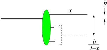
Figure 1: A three-quark configuration in the mixed representation of definite transverse position and definite plus-momentum. $x$ denotes the plus-momentum fraction of the upper quark with respect to the nucleon. The dashed line indicates the center of momentum of the two lower quarks and the thick solid line the center of momentum of the proton.

Just as the usual quark densities, GPDs depend on the factorization scale $\mu$ at which the partons are resolved. For $\xi=0$ the evolution in $\mu$ is described by the usual DGLAP equation, which for the valence combination $H_{v}^{q}$ reads

$$\mu^{2}\frac{{\rm d}}{{\rm d}\mu^{2}}H_{v}^{q}(x,t,\mu^{2})=\int_{x}^{1}\frac{{\rm d}z}{z}\,\Big{[}P\Big{(}\frac{x}{z}\Big{)}\Big{]}_{+}H_{v}^{q}(z,t,\mu^{2})\>,$$ (7)

where $[~{}]_{+}$ denotes the usual plus-distribution, and where the kernel reads $P(z)=\frac{\alpha_{s}}{2\pi}\,C_{F}\frac{1+z^{2}}{1-z}$ at leading order in the strong coupling. We note that the situation for $\mu^{2}\ll-t$ is rather subtle; it will be discussed in some detail in Sect. 7.2. Dividing (7) by $H_{v}^{q}(x,t)$ and subsequently taking the derivative in $t$ at $t=0$ we obtain an evolution equation for the average impact parameter:

$$\mu^{2}\frac{{\rm d}}{{\rm d}\mu^{2}}\langle\mbox{\boldmath{$b$}}^{2}\rangle^{q}_{x}=-\frac{1}{q_{v}(x)}\int_{x}^{1}\frac{{\rm d}z}{z}\,P\Big{(}\frac{x}{z}\Big{)}\,q_{v}(z)\Big{[}\langle\mbox{\boldmath{$b$}}^{2}\rangle^{q}_{x}-\langle\mbox{\boldmath{$b$}}^{2}\rangle^{q}_{z}\Big{]},$$ (8)

where the plus-prescription is no longer needed since the term in square brackets vanishes at $z=x$. We see that the average impact parameter decreases with $\mu$ for all $x$, provided that $\langle\mbox{\boldmath{$b$}}^{2}\rangle^{q}_{x}$ is a decreasing function of $x$.

Notice that the right-hand sides of (2) must be evaluated at a particular resolution scale $\mu$, whereas the left-hand sides are the form factors of a conserved current and hence independent of the scale $\mu$ where the current is renormalized. Physically speaking, the transverse distribution of quarks of a given momentum fraction $x$ is modified by the parton splitting processes that underly DGLAP evolution. It hence depends on the spatial resolution $1/\mu$ at which quarks are probed, whereas the transverse distribution of charge described by the electromagnetic form factors does not [28].

For the quark helicity dependent GPDs we define the valence combination

$$\widetilde{H}_{v}^{q}(x,t,\mu^{2})=\widetilde{H}^{q}(x,t,\mu^{2})-\widetilde{H}^{q}(-x,t,\mu^{2})\>,$$ (9)

whose forward limit is $\Delta q_{v}(x)=\Delta q(x)-\Delta\bar{q}(x)$. The impact parameter distribution $\Delta q_{v}(x,\mbox{\boldmath{$b$}})$ is then defined in analogy to (3) and again can be interpreted as a difference of probability densities in $x$ and $b$ space. It has a wave function representation akin to (5), with an extra minus sign in front of the squared wave function if the struck quark or antiquark has negative helicity. The evolution of $\widetilde{H}_{v}^{q}$ in the scale $\mu$ is described by a DGLAP equation as in (7), with an evolution kernel that is identical to the one for $H_{v}^{q}$ at leading order in $\alpha_{s}$. The properties of the proton helicity flip GPD $E$ will be discussed in Sect. 5.

3 A parameterization for the unpolarized GPD $H_{v}(x,t)$

3.1 Physical motivation

We now develop a parameterization for $H_{v}^{u}(x,t)$ and $H_{v}^{d}(x,t)$. For its functional form we will use theoretical guidance in the regions of very small and very large $x$ and then attempt a suitable interpolation for intermediate $x$. We will fit this parameterization to the data on the nucleon Dirac form factors $F_{1}^{p}(t)$ and $F_{1}^{n}(t)$.

For small $t$ and very small $x$ one can expect Regge behavior of $H_{v}(x,t)$, employing the same argument as in the well-known case of forward parton densities [31]. The simplest form of Regge behavior is the dominance of a single Regge pole,

$$H_{v}(x,t)\sim c(t)\,\Big{(}\frac{x_{0}}{x}\Big{)}^{\alpha(t)}=\Big{(}\frac{x_{0}}{x}\Big{)}^{\alpha(0)}\,\exp\Bigg{[}\Big{(}\alpha^{\prime}\log\frac{x_{0}}{x}+b_{0}\Big{)}\,t\,\Bigg{]},$$ (10)

where in the second step we have used a simple parameterization $c(t)=\exp(b_{0}\,t)$ for the small-$t$ region and a linear form of the Regge trajectory $\alpha(t)=\alpha(0)+\alpha^{\prime}t$. The leading Regge trajectories with the quantum numbers of $H_{v}$ are those of the $\omega$ and the $\rho$. They can be phenomenologically determined from suitable hadronic cross sections and from the Chew-Frautschi plot (showing the spin of a meson versus its squared mass, which we take from [32]). From the masses of $\omega(782)$ and $\omega_{3}(1670)$ one obtains a linear trajectory $\alpha_{\omega}(t)=0.42+0.95\,{\rm GeV}^{-2}\,t$, whose intercept at $t=0$ agrees well with the value extracted from $\sigma_{\rm{tot}}(pp)-\sigma_{\rm{tot}}(p\bar{p})$ in [33]. The masses of $\rho(770)$ and $\rho_{3}(1690)$ give a linear trajectory $\alpha_{\rho}(t)=0.48+0.88\,{\rm GeV}^{-2}\,t$, in good agreement with the intercept from $\sigma_{\rm{tot}}(\pi^{-}p)-\sigma_{\rm{tot}}(\pi^{+}p)$ and with the trajectory extracted from the data on $d\sigma/dt(\pi^{-}p\to\pi^{0}n)$ up to about $|t|\approx 0.3\,{\rm GeV}^{2}$ [34].

We emphasize that (10) is not a prediction of Regge theory, but rather corresponds to a simple form of Regge phenomenology: on one hand one expects subleading Regge trajectories to become important if $x$ is not sufficiently small, and on the other hand the importance of Regge cuts, which lead to a more complicated behavior on $x$ and $t$, is notoriously difficult to determine without further assumptions. To assess how well the ansatz (10) fares at $t=0$ we have investigated the CTEQ6M parton densities [20] at $\mu=2\,{\rm GeV}$ and found that for $10^{-5}<x<10^{-2}$ one has $u_{v}+d_{v}\approx x^{-0.435}$ and $(u_{v}-d_{v})/(u_{v}+d_{v})\approx x^{-0.07}$, both within $1\%$ accuracy. Scanning the 40 sets of parton densities given by CTEQ as error estimates, we found an exponent in the power-law for $u_{v}+d_{v}$ between $-0.38$ and $-0.495$ and a corresponding exponent for $(u_{v}-d_{v})/(u_{v}+d_{v})$ between $-0.165$ and $0.13$. Similar values are found when taking the distributions at scales $\mu=1\,{\rm GeV}$ or $\mu=4\,{\rm GeV}$. We conclude that a simple Regge pole ansatz with an intercept taken from the phenomenology of soft hadronic interactions is in fair agreement with valence quark distributions at low factorization scale, and assume in the following that this description generalizes to small finite $-t$. Note that the form (10) translates into an average impact parameter $\langle\mbox{\boldmath{$b$}}^{2}\rangle_{x}$ diverging like $\log(1/x)$ at small $x$. A physical mechanism that gives such a behavior is Gribov diffusion, the generation of small-$x$ partons through a cascade of branching processes [35].

As $x$ increases, the struck parton takes more and more weight in the center of momentum $\sum_{i}x_{i}\mbox{\boldmath{$b$}}_{i}$ of all partons, so that the distribution in $b$ should become more and more narrow [36]. This means that the $t$-dependence of GPDs should become less steep with increasing $x$. If the average distance $d_{q}(x)$ between the struck quark and the center of momentum of the spectators is to remain finite, which one may expect for a system subject to confinement, then $\langle\mbox{\boldmath{$b$}}^{2}\rangle_{x}$ must vanish at least like $(1-x)^{2}$ in the limit $x\to 1$ [37]. The actual limiting behavior of $\langle\mbox{\boldmath{$b$}}^{2}\rangle_{x}$ in QCD remains unknown. Certainly the impact parameter dependence of GPDs at large $x$ contains interesting information about the dynamics of confinement, and we shall see how much information on this dependence can be extracted from existing form factor data.

In our parameterization we will make an exponential ansatz for the $t$-dependence:

$$H_{v}^{q}(x,t)=q_{v}(x)\exp{[tf_{q}(x)]}\>.$$ (11)

The function $f_{q}(x)$ parameterizes how the profile of the quark distribution in the impact parameter plane changes with $x$, as is readily seen from

$$q_{v}(x,\mbox{\boldmath{$b$}})=\frac{1}{4\pi}\,\frac{q_{v}(x)}{f_{q}(x)}\,\exp\Bigg{[}-\frac{\mbox{\boldmath{$b$}}^{2}}{4f_{q}(x)}\Bigg{]}\>,\qquad\qquad\langle\mbox{\boldmath{$b$}}^{2}\rangle^{q}_{x}=4f_{q}(x)\>.$$ (12)

Apart from being suitable for analytic calculations, an exponential $t$-dependence of $H_{v}^{q}(x,t)$ guarantees that $q_{v}(x,\mbox{\boldmath{$b$}})$ is positive. It ensures a rapid falloff at any $x$ as $-t$ becomes large, and it readily matches with the Regge form (10) for small $x$ and $-t$ if we impose

$$f_{q}(x)\to\alpha^{\prime}\log\frac{1}{x}+B_{q}\qquad\qquad\mbox{for~{}}x\to 0\>.$$ (13)

The $t$-slope at $x=x_{0}$ is obtained as $b_{0}=\alpha^{\prime}\log(1/x_{0})+B_{q}$. In our fits we will explore a possible flavor dependence of $B_{q}$ but keep $\alpha^{\prime}$ flavor independent, as suggested by Regge phenomenology. We are aware that our exponential ansatz (11) has no rigorous theoretical backing, and we shall explore alternative forms of the $t$-dependence in Sect. 3.6. Let us emphasize already here that we cannot trust the detailed form of our extracted GPDs in the region $-t\gg 1/f_{q}(x)$, where according to (11) they are exponentially small and thus give only a tiny contribution to the form factor integrals (2). In particular we claim no validity of our ansatz at $-t$ of several $\,{\rm GeV}^{2}$ and very small $x$, where its motivation from Regge phenomenology does indeed not apply.

For large $x$ one can expect that the overlap representation (5) is dominated by Fock states with few partons. In [5] we have evaluated GPDs from model wave functions for the lowest Fock states, whose dependence on the transverse parton momenta or impact parameters was taken as Gaussian,

$$\psi\propto\exp\Bigg{[}-a^{2}\sum_{i}\frac{\mbox{\boldmath{$k$}}_{i}^{2}}{x_{i}}\,\Bigg{]}\>,\qquad\qquad\tilde{\psi}\propto\exp\Bigg{[}-\frac{1}{4a^{2}}\sum_{i}x_{i}^{\phantom{.}}\mbox{\boldmath{$b$}}_{i}^{2}\,\Bigg{]}\>,$$ (14)

a form going back to [38] and explored in detail for the nucleon in [39]. With a parameter $a^{2}=0.72\,{\rm GeV}^{-2}$ or somewhat larger, this model allowed a fair description of unpolarized and polarized $u$ and $d$ quark densities for $x\raisebox{-4.0pt}{$\,\stackrel{{\scriptstyle\textstyle>}}{{\sim}}\,$}0.6\mbox{~{}to~{}}0.7$ and of $F_{1}^{p}(t)$ for $-t\raisebox{-4.0pt}{$\,\stackrel{{\scriptstyle\textstyle>}}{{\sim}}\,$}4\,{\rm GeV}^{2}$. The resulting GPDs at $\xi=0$ take the form given in (11) and (12) with $\langle\mbox{\boldmath{$b$}}^{2}\rangle_{x}=2a^{2}(1-x)/x$. The average distance between the struck quark and the spectators hence diverges like $d_{q}(x)\sim(1-x)^{-1/2}$ in the limit $x\to 1$. Indeed the impact parameter form of the model wave functions (14) allows $\mbox{\boldmath{$b$}}_{i}^{2}$ to grow like $1/x_{i}$ when the spectators become soft. In the limit $x\to 1$ such a behavior is difficult to reconcile with confinement as was pointed out in [37], and one aim of our study here is to explore quantitatively at which $x$ the behavior of such wave functions becomes physically suspect. In our ansatz (11) for the valence GPDs we will impose the constraint

$$f_{q}(x)\to A_{q}(1-x)^{n}\qquad\qquad\mbox{for~{}}x\to 1\>,$$ (15)

either with $n=1$ as in the model just discussed, or with $n=2$, which corresponds to $d_{q}(x)$ tending to a constant at $x=1$.

The ansatz (11) must be made at a particular factorization scale $\mu$ and may work better for some scales than for others. Let us see that the limiting behavior we take for $\langle\mbox{\boldmath{$b$}}^{2}\rangle_{x}$ at small and at large $x$ retains its form under leading-order DGLAP evolution. To be more precise, let us first assume that $\langle\mbox{\boldmath{$b$}}^{2}\rangle_{x}\approx 4\alpha^{\prime}\log(1/x)+4B$ and $q_{v}(x)\approx cx^{-\alpha}$ with $\alpha>0$ at small $x$ and for a given $\mu$. We need not take the mathematical limit of $x\to 0$ but only require these forms to be good approximations in a range of $x$ where the small-$x$ approximations of the following arguments are numerically adequate. With the evolution equation (8) for $\langle\mbox{\boldmath{$b$}}^{2}\rangle_{x}$ and the leading-order evolution kernel we have

$$\mu^{2}\frac{{\rm d}}{{\rm d}\mu^{2}}\langle\mbox{\boldmath{$b$}}^{2}\rangle_{x}\approx\frac{\alpha_{s}C_{F}}{2\pi}\int_{x}^{1}{\rm d}z\Bigg{[}1+\Big{(}\frac{x}{z}\Big{)}^{2}\Bigg{]}\frac{q_{v}(z)}{q_{v}(x)}\,\frac{\langle\mbox{\boldmath{$b$}}^{2}\rangle_{x}-\langle\mbox{\boldmath{$b$}}^{2}\rangle_{z}}{x-z}\>.$$ (16)

Let $\delta$ be a fixed value of $x$ below which $q_{v}(x)$ and $\langle\mbox{\boldmath{$b$}}^{2}\rangle^{q}_{x}$ can be approximated as stated above. For $z>\delta$ the integrand behaves like $x^{\alpha}\log x$ for $x\to 0$, so that the integral over $z$ from $\delta$ to 1 gives a vanishing contribution to the right-hand side. We can hence approximate

$$\mu^{2}\frac{{\rm d}}{{\rm d}\mu^{2}}\langle\mbox{\boldmath{$b$}}^{2}\rangle_{x} \approx -\frac{\alpha_{s}C_{F}}{2\pi}\int_{x}^{\delta}{\rm d}z\Bigg{[}1+\Big{(}\frac{x}{z}\Big{)}^{2}\Bigg{]}\Big{(}\frac{x}{z}\Big{)}^{\alpha}\,\frac{4\alpha^{\prime}\log(z/x)}{z-x}$$ (17)

$$= -4\alpha^{\prime}\,\frac{\alpha_{s}C_{F}}{2\pi}\int_{1}^{\delta/x}{\rm d}u\,(1+u^{-2}\,)\,u^{-\alpha}\,\frac{\log u}{u-1}\>,$$

which tends to a negative constant for $x\to 0$. The divergent part $4\alpha^{\prime}\log(1/x)$ of $\langle\mbox{\boldmath{$b$}}^{2}\rangle_{x}$ is hence $\mu$ independent, whereas the constant $4B$ will decrease with $\mu$. Our argument can be generalized to other forms of $q_{v}(x)$ at small $x$, for instance to a sum $\sum_{k}c_{k}x^{-\alpha_{k}}$ with $\alpha_{k}>0$.

Concerning the large-$x$ behavior, one can show that a form $\langle\mbox{\boldmath{$b$}}^{2}\rangle_{x}\approx 4A(1-x)^{n}$ with $n>0$ is stable under leading-order DGLAP evolution, provided that the forward densities at a given $\mu$ behave as $q_{v}(x)\sim(1-x)^{\beta}$. More precisely, the coefficient $A$ decreases with $\mu$, whereas the power $n$ remains stable. To see this one starts with the evolution equation (16), replaces $q_{v}$ and $\langle\mbox{\boldmath{$b$}}^{2}\rangle$ on the right-hand side with the approximations just given, and Taylor expands the evolution kernel to leading order in $(1-x)$. The result is

$$\mu^{2}\frac{{\rm d}}{{\rm d}\mu^{2}}\langle\mbox{\boldmath{$b$}}^{2}\rangle_{x}\approx-4A(1-x)^{n}\,\frac{\alpha_{s}C_{F}}{\pi}\int_{0}^{1}{\rm d}v\,v^{\beta}\,\frac{1-v^{n}}{1-v}\>.$$ (18)

The leading $x$-dependence is hence in $(1-x)^{n}$ on both sides, and one obtains an equation for the evolution of its coefficient $4A$ with $\mu$. Our finding is in line with a numerical study of pion GPDs by Vogt [40], who found that in a finite interval of large $x$ the form (11) with $f(x)=\frac{1}{2}a^{2}(1-x)/x$ is approximately stable under DGLAP evolution, with a moderate decrease with $\mu$ of the parameter $a^{2}(\mu)$. For the Gaussian model wave functions giving this form of GPDs, a decrease of $a^{2}$ entails a decreasing probability of the corresponding lowest Fock states. This is in agreement with physical intuition: at higher resolution scale $\mu$ one resolves more and more partons in the hadron, and to find a configuration with only a few partons becomes less likely.

The exponential $t$-dependence (11) of GPDs is generally not stable under DGLAP evolution. To see this let us consider the Taylor expansion

$$\log H_{v}^{q}(x,t)=\log q_{v}(x)+t\Bigg{[}\frac{\partial}{\partial t}\log H_{v}^{q}(x,t)\Bigg{]}_{t=0}+\frac{1}{2}t^{2}\Bigg{[}\frac{\partial^{2}}{\partial t^{2}}\log H_{v}^{q}(x,t)\Bigg{]}_{t=0}+\ldots\>,$$ (19)

which ends after the linear term if the $t$-dependence of $H_{v}^{q}$ is exponential. Dividing (7) by $H_{v}^{q}(x,t)$ and taking the second derivative in $t$ we obtain the scale dependence of the quadratic term in (19) as

$$\mu^{2}\frac{{\rm d}}{{\rm d}\mu^{2}}\,\Bigg{[}\frac{\partial^{2}}{\partial t^{2}}\log H_{v}^{q}(x,t)\Bigg{]}_{t=0}=\frac{1}{q_{v}(x)}\int_{x}^{1}\frac{{\rm d}z}{z}\,P\Big{(}\frac{x}{z}\Big{)}\,q_{v}(z)$$ (20)

$${}\times\Bigg{[}\Big{(}\frac{\partial}{\partial t}\log H_{v}^{q}(z,t)-\frac{\partial}{\partial t}\log H_{v}^{q}(x,t)\Big{)}^{2}+\frac{\partial^{2}}{\partial t^{2}}\Big{(}\log H_{v}^{q}(z,t)-\log H_{v}^{q}(x,t)\Big{)}\Bigg{]}_{t=0}.$$

If at a given scale $\mu$ the $t$-dependence is exponential, then the right-hand side of (20) is positive so that the quadratic term in (19) becomes positive as one evolves to a higher scale.

In the small-$x$ limit we do however find approximate stability under evolution. With the same assumptions and approximations that led to (17) we get

$$\mu^{2}\frac{{\rm d}}{{\rm d}\mu^{2}}\,\Bigg{[}\frac{\partial^{2}}{\partial t^{2}}\log H_{v}^{q}(x)\Bigg{]}_{t=0}\approx(\alpha^{\prime})^{2}\,\frac{\alpha_{s}C_{F}}{2\pi}\int_{1}^{\delta/x}{\rm d}u\,(1+u^{-2}\,)\,u^{-\alpha}\,\frac{(\log u)^{2}}{u-1}$$ (21)

if the second derivative in $t$ of $\log H_{v}^{2}$ vanishes at the scale $\mu$. The change with $\mu$ of the quadratic term in the Taylor expansion (19) is then of order $(t\alpha^{\prime})^{2}$. For moderate values of $t\alpha^{\prime}$ this is small compared with the linear term $t\alpha^{\prime}\log(1/x)$.

In the large-$x$ limit we get in analogy to (18)

$$\mu^{2}\frac{{\rm d}}{{\rm d}\mu^{2}}\,\Bigg{[}\frac{\partial^{2}}{\partial t^{2}}\log H_{v}^{q}(x)\Bigg{]}_{t=0}\approx A^{2}(1-x)^{2n}\frac{\alpha_{s}C_{F}}{\pi}\int_{0}^{1}{\rm d}v\,v^{\beta}\,\frac{(1-v^{n})^{2}}{1-v}$$ (22)

if at the scale $\mu$ the $t$-dependence of $H_{v}^{q}$ is exponential. The change with $\mu$ of the quadratic term in the Taylor expansion (19) is then parametrically of order $(tA)^{2}(1-x)^{2n}$. This is not small compared with the linear term $tA(1-x)^{n}$ if the latter is of order $1$. Numerically however the $v$-integral in (22) is rather small, namely $0.05$ for $n=1$ and $0.14$ for $n=2$ if $\beta=3$. For large $x$ we thus find that the departure from the exponential behavior (11) under evolution should not be too strong in the $t$-region where the exponent $tf(x)$ does not take too large negative values. This is again in agreement with the numerical study of Vogt [40] mentioned above.

So far we have considered the valence combination $H_{v}$ of quark GPDs. Let us briefly comment on what one would expect for the “sea quark” distributions $H(x,t)$ at $x<0$. At large $x$, the wave function overlap picture suggests a different impact parameter or $t$-dependence than for the valence distribution, because sea quark distributions require Fock states with at least one $q\bar{q}$ pair in addition to the minimal three-quark configuration. In the small-$x$ limit one may expect a form as in (10) at low scale $\mu$, given that the leading $\rho$, $\omega$, $a_{1}$ and $f_{1}$ Regge trajectories all have approximately the same $\alpha(t)$. The situation for sea quarks is however more complicated because the singlet combination $\sum_{q}[H^{q}(x,t)-H^{q}(-x,t)]$ mixes under DGLAP evolution with the gluon GPD $H^{g}(x,t)$, whose small-$x$ behavior is dominated by Pomeron exchange. It is well-known that for the forward quark densities this leads to a drastic modification of the small-$x$ behavior as one increases the scale $\mu$ even to moderate values of a few GeV, and one cannot exclude similarly strong modifications for the parameter $\alpha^{\prime}$ of sea quarks. There is no data for form factors which might constrain the sea quark GPDs at $\xi=0$ in a similar fashion as the electromagnetic form factors constrain $H_{v}^{q}$. To investigate the sea quark sector one will rather rely on measurements of exclusive processes like deeply virtual Compton scattering or meson electroproduction at small $t$, where GPDs at nonzero $\xi$ are accessible.

3.2 Selecting a profile function

The assumption of an exponential $t$-dependence and the parameterization for the profile function $f_{q}(x)$ in (11) represent a source of theoretical bias, which translates into a systematic error in the determination of GPDs from experimental data. To gain a feeling for this error we will carefully compare different parameterizations. Our criteria for a good parameterization are:

• simplicity,

• consistency with theoretical and phenomenological constraints,

• easy physical interpretation of parameters, if possible,

• stability with respect to variations of the forward parton densities.

In this section we discuss a few examples, including the default parameterization we will use in the remainder of the paper. For each parameterization we fix the free parameters by a $\chi^{2}$ fit to the experimental data on $F_{1}^{p}$ and $F_{1}^{n}$. For the forward densities $q_{v}(x)$ we will use the CTEQ6M distributions [20] at $\mu=2\,{\rm GeV}$ as a default, where the choice of scale is a compromise between being large enough for $q_{v}(x)$ to be rather directly fixed by data and small enough to make contact with soft physics like conventional Regge phenomenology. Tables with the results of our fits are collected in App. B, and details of our data selection and error treatment are given in App. A.

The simplest form of the profile function $f_{q}(x)$ satisfying our constraints (13) and (15) with $n=1$ is actually $f_{q}(x)=\alpha^{\prime}\log(1/x)$ itself. Such a Regge behavior of the GPDs has already been mentioned in [13] and [36] and was explored in some detail in [18]. One can however not expect this simple form, where one and the same parameter describes physics at small and large $x$, to work beyond a rough accuracy. Note that even in the small-$x$ limit this form is special since it fixes the parameter $b_{0}$ in (10) to be $\alpha^{\prime}\log(1/x_{0})$. As a simple extension of this ansatz one may try

$$f_{q}(x)=\alpha^{\prime}\log\frac{1}{x}+(A_{q}-\alpha^{\prime})(1-x)\>,$$ (23)

which is still in agreement with (13) and (15). A very good fit ($\chi^{2}/\mathrm{d.o.f.}=1.34$) of the nucleon Dirac form factors can then be obtained with three free parameters, $\alpha^{\prime}$, $A_{u}$ and $A_{d}$, see Table 6. The fitted value $\alpha^{\prime}=(1.38\pm 0.01)\,{\rm GeV}^{-2}$ is however significantly larger than what Regge phenomenology would lead one to expect. This disagreement becomes even stronger if we take the forward parton densities at $\mu=1\,{\rm GeV}$ instead of $2\,{\rm GeV}$. The fit then gives $\alpha^{\prime}=(1.65\pm 0.02)\,{\rm GeV}^{-2}$ with $\chi^{2}/\mathrm{d.o.f.}=1.14$.

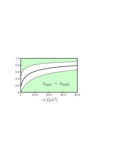
Figure 2: Region of $x$ (white region) which accounts for $90\%$ of $F_{1}^{p}(t)$ in the best fit to (23) at $\mu=2\,{\rm GeV}$. The upper and lower shaded $x$-regions each account for $5\%$ of $F_{1}^{p}(t)$, see (24). The thick line shows the average $\langle x\rangle_{t}$ defined in (25).

To better understand the situation we first determine the region of $x$ in (2) to which our fit is actually sensitive. To this end we consider the minimal and maximal value of $x$ which is needed to account for $95\%$ of the form factor in the sum rule,

$$\int\limits_{x_{\rm min}(t)}^{1}{\rm d}x\,\sum_{q}e_{q}\,H^{q}_{v}(x,t) = \mbox{95\%}\cdot F_{1}^{p}(t)\>,$$

$$\int\limits^{x_{\rm max}(t)}_{0}{\rm d}x\,\sum_{q}e_{q}\,H^{q}_{v}(x,t) = \mbox{95\%}\cdot F_{1}^{p}(t)\>,$$ (24)

where $e_{u}=\frac{2}{3}$ and $e_{d}=-\frac{1}{3}$. We concentrate on the proton form factor for this purpose, which is the most important input to our fit given the available data. A related quantity is the average value of $x$ in the form factor integral, given by

$$\langle x\rangle_{t} = \frac{\int_{0}^{1}{\rm d}x\,\sum_{q}e_{q}\,x\,H^{q}_{v}(x,t)}{\int_{0}^{1}{\rm d}x\,\sum_{q}e_{q}\,H^{q}_{v}(x,t)}\ .$$ (25)

In Fig. 2 we show $x_{\rm min}$, $x_{\rm max}$ and $\langle x\rangle_{t}$ obtained for the best fit to (23) as a function of $|t|$. The relevant $x$-range moves towards higher values for increasing momentum transfer. With the existing data on $F_{1}^{p}$ going up to $-t=31.2\,{\rm GeV}^{2}$, the region of $x$ where the profile function can be constrained by our fit goes up to about 0.8 or 0.9. On the other extreme we have $x_{\rm min}\approx 1.4\times 10^{-3}$ at $t=0$. Clearly, the form factor integrals are only sensitive to the small-$x$ behavior of $H_{v}^{q}$ if $t$ is also small, as we anticipated below (13).

Let us now see which of the parameters in our fit is most important in the profile function at given $x$. In Fig. 3 we show the quantities

$$l_{q}(x)=\frac{f_{q}(x)}{\log\frac{1}{x}}$$ (26)

resulting from our fit, where we have divided out the factor $\log(1/x)$ in order to have a finite quantity in the limit $x\to 0$. We also show the individual contributions to $l_{q}$ from the terms $\alpha^{\prime}[\log(1/x)-(1-x)]$ and $A_{q}(1-x)$ in $f_{q}$ and see that the value of $\alpha^{\prime}$ controls the profile function in almost the entire $x$ range for $u$ quarks and in a substantial region for $d$ quarks. The fitted value of $\alpha^{\prime}$ thus reflects dynamics at both small and large $x$ (in the fit it has to find a compromise between these regions). We can hardly expect it to give a good representation of the physics in the region where Regge phenomenology is relevant, say for $x\raisebox{-4.0pt}{$\,\stackrel{{\scriptstyle\textstyle<}}{{\sim}}\,$}10^{-2}$.

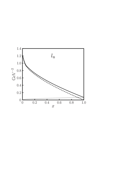
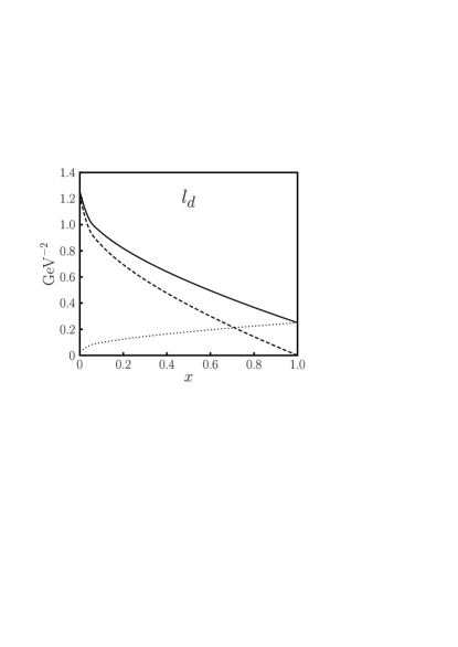
Figure 3: The function $l_{q}(x)$ from (26) for the best fit to (23) with $\mu=2\,{\rm GeV}$. The contributions from terms going with $\alpha^{\prime}$ (dashed line) and $A_{q}$ (dotted line) are shown separately.

The simplest profile function satisfying the constraints (13) and (15) with $n=2$ is $f_{q}(x)=\alpha^{\prime}(1-x)\log(1/x)$, which has been proposed in [36] and used for numerical studies in [24]. An obvious extension of this ansatz is

$$f_{q}(x)=\alpha^{\prime}(1-x)\log\frac{1}{x}+(A_{q}-\alpha^{\prime})(1-x)^{2}\>.$$ (27)

A fit with free parameters $\alpha^{\prime}$, $A_{u}$ and $A_{d}$ does not give a good description of the form factor data, see Table 6. Having an overall $\chi^{2}/\mathrm{d.o.f.}=5.25$ it systematically overshoots the $F_{1}^{p}$ data at $|t|$ above $10\,{\rm GeV}^{2}$, namely by 15% to 20% for $|t|\raisebox{-4.0pt}{$\,\stackrel{{\scriptstyle\textstyle>}}{{\sim}}\,$}20\,{\rm GeV}^{2}$. Comparing with the good fit we obtained with (23) one might conclude that the data prefers a behavior $f_{q}(x)\sim(1-x)$ over $f_{q}(x)\sim(1-x)^{2}$ at $x\to 1$, but this would be mistaken as we shall see below.

In search of a more adequate profile function we demand that

• the low-$x$ behavior of $f_{q}(x)$ should match the form (13), where we now impose the value $\alpha^{\prime}=0.9$ GeV² from Regge phenomenology,

• the high-$x$ behavior should be controlled by the parameter $A_{q}$ in (15) and not by $\alpha^{\prime}$,

• the intermediate $x$-region should smoothly interpolate between the two limits, with a few additional parameters providing enough flexibility to enable a good fit to the form factor data.

We found these requirements to be satisfied by the forms

$$f_{q}(x)=\alpha^{\prime}(1-x)^{2}\log\frac{1}{x}+B_{q}(1-x)^{2}+A_{q}\,x(1-x)$$ (28)

and

$$f_{q}(x)=\alpha^{\prime}(1-x)^{3}\log\frac{1}{x}+B_{q}(1-x)^{3}+A_{q}\,x(1-x)^{2}\>,$$ (29)

which respectively correspond to $n=1$ and $n=2$ in (15). At large $x$, the individual terms behave like $\alpha^{\prime}(1-x)^{n+2}$, $B_{q}(1-x)^{n+1}$ and $A_{q}(1-x)^{n}$, which in particular prevents the term with $\alpha^{\prime}$ from being too important in the high-$x$ region.

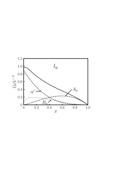
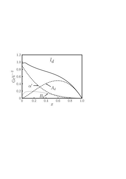
Figure 4: The function $l_{q}(x)$ from (26) for the best fit to (29) with $\mu=2\,{\rm GeV}$. The contributions from terms going with $\alpha^{\prime}$, $B_{q}$ and $A_{q}$ are shown separately.

As we see in Tables 7 and 8, a fit to either (28) or (29) with $A_{u}$, $A_{d}$ and $B_{u}=B_{d}$ as free parameters provides a good description of the form factor data. We will comment on setting $B_{u}=B_{d}$ in Sect. 3.4. In Fig. 4 we show the profile functions divided by $\log(1/x)$ obtained in the fit to (29), as well as the individual contributions from the terms with $\alpha^{\prime}$, $B_{q}$ and $A_{q}$. Our criterion that the profile function should be controlled by $\alpha^{\prime}$ at low $x$ and by $A_{q}$ at high $x$ is now well satisfied. To a lesser degree this also holds for the fit to (28), where the contribution of the $\alpha^{\prime}$ term to $f_{u}(x)$ is about $30\%$ at $x=0.7$ and $15\%$ at $x=0.8$. The sensitive region of $x$ in both fits is essentially the same as for the fit to (23), with the values of $x_{\rm max}(t)$ and $\langle x\rangle_{t}$ differing by less than 2% from those shown in Fig. 2. The difference of $x_{\rm min}(t)$ in the different fits is more pronounced at small $t$ but below 5% for $-t$ above $1\,{\rm GeV}^{2}$.

We see from Tables 7 and 8 that $f_{d}(x)$ has clearly larger errors than $f_{u}(x)$. This is a feature of all our fits (except when we force $f_{u}(x)$ and $f_{d}(x)$ to be equal) and can readily be understood from the sum rules (2). Due to the charge factors, the integrand giving $F_{1}^{p}$ is dominated by the contribution from $u$ quarks. This trend is enhanced by the fact that $u$ quarks are more abundant in the proton than $d$ quarks. For large $x$ the ratio $d_{v}/u_{v}$ of parton densities becomes very small indeed (see Fig. 9), and one can expect this trend to persist for $H_{v}^{d}/H_{v}^{u}$ at least over some range in $t$. The combination of $F_{1}^{p}$ and $F_{1}^{n}$ provides sensitivity to $d$ quarks, but data on both form factors is only available in a relatively small interval of $|t|$. Improved data on $F_{1}^{n}$ in a wider range of $t$ would be highly welcome in this context.

In Fig. 5 we show the distance $d_{q}(x)$ obtained with our fits to (28) and to (29). For $u$ quarks the results of the two fits are fully compatible within their errors up to about $x=0.75$. The $x$-region where they differ significantly is outside the range where our fit to the form factors can constrain them. For $d$ quarks the results start to differ at lower values of $x$, but their errors are significantly bigger as well. We conclude that the limiting behavior of $d_{q}(x)$ for $x\to 1$ cannot be determined by data on $F_{1}^{p}$ up to $|t|$ around $30\,{\rm GeV}^{2}$. We note that the description of $F_{1}^{p}$ at high $|t|$ is slightly better for the fit to (29) than for the one to (28), where $F_{1}^{p}(t)$ falls off a bit too fast. One should however not interpret this as a preference of the data for $n=2$ rather than $n=1$ in the power-law falloff (15) since the situation is opposite for the fits to (23) and (27), see Tables 6, 7 and 8. Which value of $n$ a fit prefers thus depends on the remaining functional dependence of $d_{q}(x)$. Without data constraining $d_{q}(x)$ for $x$ above $0.8$ we cannot determine its behavior around $x=1$.

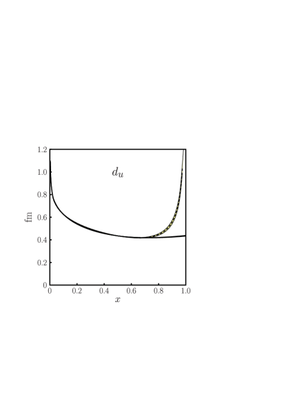
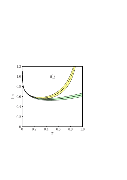
Figure 5: The distance $d_{q}(x)$ between struck quark and spectators, evaluated for the best fits to (28) (dashed line) and (29) (solid line) with $\mu=2\,{\rm GeV}$. The smallest $x$ value plotted is $5\cdot 10^{-3}$. Shaded bands indicate the $1\,\sigma$ uncertainties of the fits as explained in App. B.

We also see in Fig. 5 that $d_{u}$ from the fit with $n=1$ takes values one may suspect to be unphysically large only for $x$ above $0.9$ or so, where even the forward parton densities are barely known. Similarly, for models obtained with the Gaussian wave functions (14) and the parameters used in [39, 5], the distance $d_{q}$ stays below 1 fm for $x\raisebox{-4.0pt}{$\,\stackrel{{\scriptstyle\textstyle<}}{{\sim}}\,$}0.9$. In the kinematic range where these models have been used to describe or predict data we hence do not find them physically inconsistent. In the following we will however take the form with $n=2$ in (15), since its limiting behavior for $x\to 1$ is more plausible than the one with $n=1$. An exponent $n$ above $2$, which results in a vanishing $d_{q}$ for $x\to 1$, may also be possible [37]. Since the form factor data cannot determine $n$ we refrain however from further investigation of this point. We henceforth refer to the fit to (11) and (29) at $\mu=2\,{\rm GeV}$ as our “default fit”. Its parameters are

$$A_{u} = (1.22\pm 0.02)\,{\rm GeV}^{-2},\qquad\qquad A_{d}\>=\>(2.59\pm 0.29)\,{\rm GeV}^{-2},$$

$$B_{u} = B_{d}\>=\>(0.59\pm 0.03)\,{\rm GeV}^{-2},$$ (30)

and $\alpha^{\prime}=0.9\,{\rm GeV}^{-2}$, with full details given in App. B. Note that in this fit the parameter $A_{q}$ has a simple physical interpretation as the limit of $d_{q}^{\,2}/4$ for $x\to 1$. To a good approximation it also gives the value of this quantity over a finite range of large $x$.

3.3 Features of the default fit

In Fig. 6 we compare the form factor data with the result of our default fit, whose parametric uncertainties are shown by the shaded bands. To have a clear representation of the data at large $t$ we have scaled the form factors with $t^{2}$. The quality of the fit at smaller $t$ is better seen from the “pull”, defined as $[F_{1}({\rm data})/F_{1}({\rm fit})-1]$ and shown in Fig. 7. Our fitted GPDs describe $F_{1}^{p}$ within 5% for $-t$ up to $27\,{\rm GeV}^{2}$, only the last data point at $-t=31.2\,{\rm GeV}^{2}$ has a larger pull. Apart from the data point at $-t=0.255\,{\rm GeV}^{2}$ with its huge errors, our fit describes $F_{1}^{n}$ within $25\%$. A detailed inspection reveals that a large contribution to $\chi^{2}$ is due to five data points in the sample of [41], with $0.18\,{\rm GeV}^{2}\leq-t\leq 0.86\,{\rm GeV}^{2}$. The relative errors for these data are only about $1\%$, which is below the accuracy we are aiming at. We are hence not worried by the comparatively high $\chi^{2}$ value found in our fit.

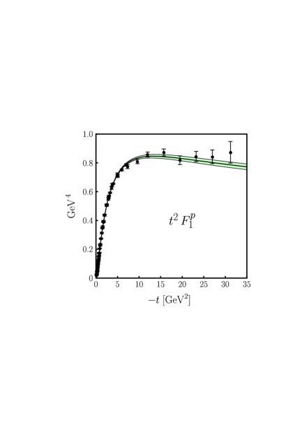
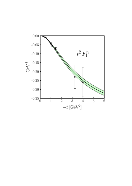
Figure 6: Results for the Dirac form factor of proton and neutron with our default fit, defined by (11) and (29) with the parameters (3.2) and the valence quark densities evaluated at scale $\mu=2\,{\rm GeV}$. The solid lines represent the best fit, and the error bands represent the $1\,\sigma$ uncertainties of the fit as explained in App. B. Details on the form factor data and their errors are given in App. A.

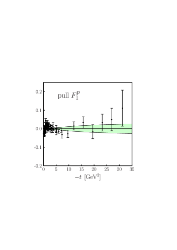
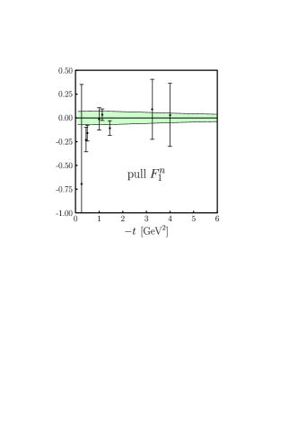
Figure 7: The pull $[F_{1}({\rm data})/F_{1}({\rm fit})-1]$ for our default fit to the Dirac form factors of the nucleon. The error bands represent the $1\,\sigma$ fit uncertainties relative to the best fit.

The distance $d_{q}(x)$ between the struck quark and the spectators shown in Fig. 5 is one of our main physics results. Our analysis provides the first data-driven determination of this important quantity. It exhibits a significant decrease when going from small to intermediate $x$. We will comment on the increase of $d_{d}(x)$ for $x\raisebox{-4.0pt}{$\,\stackrel{{\scriptstyle\textstyle>}}{{\sim}}\,$}0.4$ at the end of Sect. 3.4.

In Fig. 8 we show the square root of the average impact parameters $\langle\mbox{\boldmath{$b$}}^{2}\rangle_{x}$ for the sum and the difference of $u$ and $d$ quark distributions, defined as in (4) with $H_{v}^{q}$ replaced by $H_{v}^{u}\pm H_{v}^{d}$. That $\langle\mbox{\boldmath{$b$}}^{2}\rangle_{x}$ comes out somewhat bigger for $u+d$ than for $u-d$ reflects that $\langle\mbox{\boldmath{$b$}}^{2}\rangle^{u}_{x}<\langle\mbox{\boldmath{$b$}}^{2}\rangle^{d}_{x}$ in our fit. The points shown in the figure are results from an evaluation of moments $\int_{-1}^{1}{\rm d}x\,x^{m}[H^{u}(x,t)\pm H^{d}(x,t)]$ in lattice QCD [11]. A quantitative comparison of the two results must be made with due caution. For one thing, the values of $x$ in the lattice calculation have been estimated from the ratios of successive moments in $x$ at $t=0$. We could of course avoid this problem by directly comparing our results for $x$ moments with those obtained on the lattice. More importantly, however, the lattice calculation was performed for a pion mass of 870 MeV, and an extrapolation to the physical pion mass has not been attempted in [11]. Indeed, the falloff in $t$ of $(F_{1}^{u}+F_{1}^{d})$ and $(F_{1}^{u}-F_{1}^{d})$ obtained in that calculation [10, 11] is too slow to correctly describe the data for $F_{1}^{p}$ and $F_{1}^{n}$. Together with the uncertainties inherent in our phenomenological extraction, we nevertheless find the overall agreement of the results in Fig. 8 remarkable.

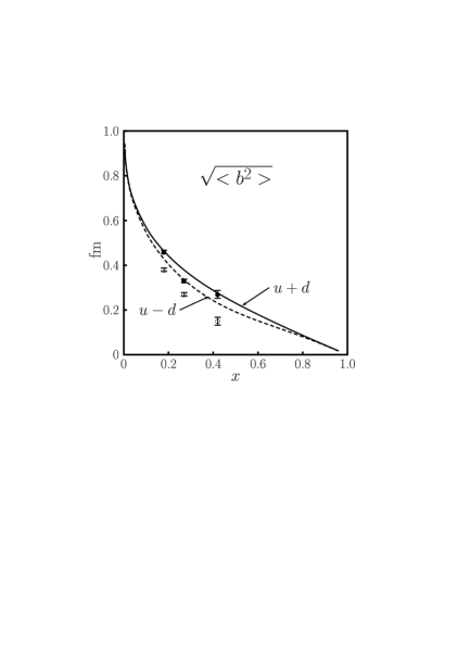
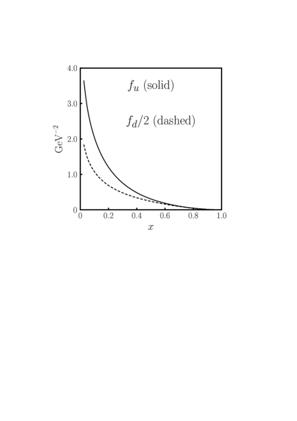
Figure 8: Left: Square root of the average impact parameters $\langle\mbox{\boldmath{$b$}}^{2}\rangle_{x}$ for the sum and the difference of $u$ and $d$ quark distributions obtained in our default fit, compared with lattice QCD results from [11]. The smallest $x$-value plotted is $5\cdot 10^{-3}$. Right: The profile functions $f_{u}$ and $f_{d}$ obtained in our default fit (29) (solid) with $\mu=2\,{\rm GeV}$. For better visibility $f_{d}$ has been scaled by a factor $1/2$. The smallest $x$-value plotted is $2.5\cdot 10^{-2}$.

In Fig. 8 we also show the profile functions $f_{u}$ and $f_{d}$ themselves. The scale controlling the decrease of $H_{v}^{q}(x,t)$ with $t$ is seen to depend very strongly on $x$, not only in the regions of very large or very small $x$ but also when going from, say, $x=0.1$ to $x=0.3$.

3.4 Variations of the fit

The $1\,\sigma$ errors quoted in our tables and the associated error bands in the figures reflect the uncertainty on the free parameters in a given parameterization of the GPDs, but not the uncertainty due to the choice of parameterization. In order to obtain a better feeling how significant various features of our default fit are, we have tested their stability under several modifications of the fit.

To investigate the difference between the profile functions for $u$ and $d$ quarks we have fitted the data to the form (29) with or without setting $B_{u}=B_{d}$ and $A_{u}=A_{d}$, see Table 8. The fit with all four parameters free leads only to a slightly better description of the data than our default fit with $B_{u}=B_{d}$. The fitted parameters are compatible with those in the default fit at $2\,\sigma$ level, but the errors on $A_{d}$ and $B_{d}$ are much larger. We find that the presently available data on $F_{2}^{n}$ do not warrant two free parameters for $d$ quarks. Note that although $B_{u}>B_{d}$ in this fit, the resulting function $f_{u}(x)$ only becomes larger than $f_{d}(x)$ for $x<0.1$, where the difference between the two functions is at most 5%. Already at $x=0.3$ the ratio $f_{d}/f_{u}$ has grown to a value of 1.4, to be compared with 1.3 in our default fit. A fit where we impose both $A_{u}=A_{d}$ and $B_{u}=B_{d}$ cannot adequately describe the neutron data. The $\chi^{2}$ in this subsample is 74 for 8 data points, and the fit result for $|F_{1}^{n}|$ undershoots the data by at least $30\%$ for $-t\geq 1\,{\rm GeV}^{2}$. The same happens if we take the profile function (28) with $f_{u}(x)=f_{d}(x)$, see Table 7. A three-parameter fit to (29) with the constraint $A_{u}=A_{d}$ finds $B_{u}<B_{d}$. It still undershoots the data on $|F_{1}^{n}|$ for $-t\geq 1\,{\rm GeV}^{2}$, although not as badly as the fit where both $A_{u}=A_{d}$ and $B_{u}=B_{d}$.

We conclude that if we insist on having a good description of both proton and neutron form factors, we need $f_{d}(x)>f_{u}(x)$ at moderate to large values of $x$. This implies that the suppression of $d$ compared with $u$ quarks seen in the forward parton densities at high $x$ becomes even stronger for $H_{v}^{d}$ and $H_{v}^{u}$ as $|t|$ increases. Note that the observed rise of the form factor ratio $-F_{1}^{n}(t)/F_{1}^{p}(t)$ implies that the flavor contribution $F_{1}^{d}(t)$ decreases faster with $|t|$ than $F_{1}^{u}(t)$. This is seen by writing

$$R_{1}(t)=-\frac{2F_{1}^{n}(t)}{F_{1}^{p}(t)}=\frac{1-r_{1}(t)}{1-\frac{1}{4}\,r_{1}(t)}\,,\qquad\qquad\qquad r_{1}(t)=\frac{2F_{1}^{d}(t)}{F_{1}^{u}(t)}\,.$$ (31)

With the data giving $R_{1}\approx 0.37$ at $-t=1\,{\rm GeV}^{2}$ one has $r_{1}\approx 0.7$, which is clearly different from the value $r_{1}=1$ at $t=0$. To have $r_{1}(t)$ decreasing sufficiently fast, the damping factor $f_{q}$ in the $t$ dependence must be bigger for $H_{v}^{d}$ than for $H_{v}^{u}$ when we take the exponential form (11). The same trend is observed with the power-law dependence on $t$ we investigate in Sect. 3.6, see Table 11.

It is well known that as $x$ becomes larger, the parton densities extracted from data become more and more uncertain. In their analysis [20] CTEQ provide 40 sets of parton densities which reflect variations from their best fit results that are allowed within errors. Among these we find sets 17, 18 and 35, 36 to provide the largest deviations from the best fit parton densities at large $x$, reaching 20% for $u_{v}$ at $x=0.9$ and for $d_{v}$ at $x=0.7$ and growing well beyond $100\%$ for $d$ quarks at higher $x$. In Fig. 9 we show the corresponding ratio $d_{v}(x)/u_{v}(x)$, which is especially important for the simultaneous description of the form factors $F_{1}^{p}$ and $F_{1}^{n}$ in our fit. Repeating our default fit with these error distributions as input, we find good stability of the obtained GPDs, see Table 9. The profile functions $f_{u}$ for the error distributions deviate by at most 3% from the one for the CTEQ best fit, as well as $f_{d}$ for sets 17 and 18. With both sets 35 and 36 the ratio of $f_{d}$ obtained for the error distribution and for the CTEQ best fit grows from 1 to about 1.1 as $x$ rises from 0 to 1. The uncertainties on the forward parton densities thus hardly affect our extraction of the impact parameter profile of parton distributions as a function of $x$.

Figure 9: The ratio $d_{v}(x)/u_{v}(x)$ obtained with different sets of CTEQ6M parton distributions [20] at scale $\mu=2\,{\rm GeV}$. The largest plotted value of $x$ is $0.97$.

We have finally allowed the value of $\alpha^{\prime}$ in (29) to be selected by the fit, and in addition we have taken the forward distributions in our ansatz (11) at different scales $\mu$. The results are given in Table 10. In all cases we obtain a rather good description of the form factor data, although there is a tendency for the fits to become worse for larger $\mu$. We see that our parameterization of GPDs is reasonably flexible to cover a range of factorization scales. This also validates the analytical considerations in Sect. 3.1, which showed that in selected regions of $x$ and $t$ our functional form of GPDs is approximately stable under a change of $\mu$. The profile functions $f_{u}$ and $f_{d}$ obtained in our fits decrease with $\mu$, precisely as we expect from the evolution equation (8) for $\langle\mbox{\boldmath{$b$}}^{2}\rangle_{x}$. In Fig. 10 we show the change of parameters $\alpha^{\prime}$, $A_{u}$ and $B_{u}=B_{d}$ with $\mu$. The uncertainty on $A_{d}$ is too large to observe a clear evolution effect. The mild $\mu$ dependence in the central values of $\alpha^{\prime}$ does not contradict our general analysis in Sect. 3.1, where $\alpha^{\prime}$ describes the behavior of the profile function at very small $x$, whereas the parameter $\alpha^{\prime}$ in our ansatz for $f_{q}(x)$ is relevant in a finite $x$ interval (see Fig. 4). Given this and the uncertainties on $\alpha^{\prime}$ within Regge phenomenology, we conclude that the fitted values of this parameter confirm our assumption that the valence GPDs at small $x$ and $t$ can be described by the leading Regge trajectories known from the phenomenology of soft hadronic interactions. The results of this exercise also justifies the choice of fixing $\alpha^{\prime}$ in our default fit, although it is clear that its parametric errors underestimate the uncertainty of the profile function in the small-$x$ limit.

Figure 10: Parameters and their errors obtained in a fit to (11) and (29) with $B_{u}=B_{d}$ and forward parton distributions taken at different scales $\mu$. The corresponding parameters are given in Table 10.

To illustrate the uncertainties of our fit results due to the choice of parameterization, we show in Fig. 11 the average distances $d_{u}(x)$ and $d_{d}(x)$ obtained with selected fits, which provide good descriptions for both proton and neutron data. We see that for $u$ quarks there is little influence of the parameterization up to $x\sim 0.8$. For $d$ quarks the uncertainties are larger, due to the lack of good neutron data at higher values of $t$. The curve with the lowest values of $d_{d}(x)$ in the figure belongs to the fit in Table 8 where $A_{u}=A_{d}$ but $B_{u}\neq B_{d}$, which provides only a moderately good description of the neutron data. This is the only fit among those shown where $d_{u}$ and $d_{d}$ differ by less than $10\%$ over the entire $x$ range. In all other cases we observe in particular that $d_{d}(x)$ rises for $x$ above a certain moderate value, in order to accommodate a rise of the ratio $f_{d}/f_{u}$.

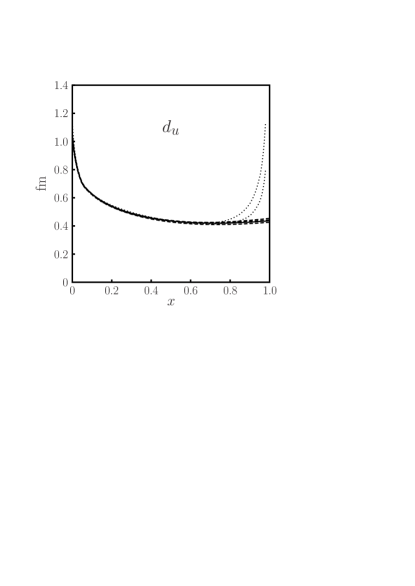
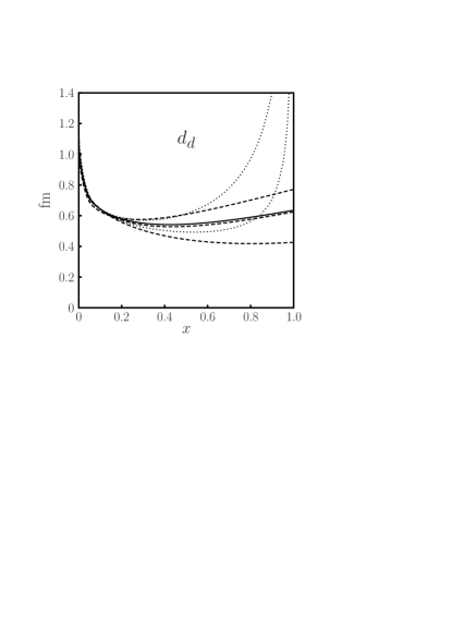
Figure 11: The average distance $d_{q}(x)$ for $u$ and $d$ quarks for selected fits. The solid lines show our default fit, and dashed lines the fits in the second and third rows of Table 8 and in the second row of Table 10. Dotted lines show the fits in the first row of Table 6 and the first row of Table 7, where $d_{q}(x)\sim(1-x)^{-1/2}$ for $x\to 1$.

3.5 Large $t$ and the Feynman mechanism

In this subsection we will see that our parameterization of GPDs enables the Feynman mechanism at large $t$, where the struck quark carries most of the nucleon momentum and thus avoids large internal virtualities of order $t$. Let us first consider $H_{v}^{q}(x,t)$ in the limit of large $x$ and take a closer look at the scaling of momenta, which we denote as shown in Fig. 12a. Defining light-cone coordinates, $v^{\pm}=(v^{0}\pm v^{3})/\sqrt{2}$ and $\mbox{\boldmath{$v$}}_{\perp}=(v^{1},v^{2})$ for any four-vector $v$, we have $x=k^{+}/p^{+}$. We choose a reference frame where $\Delta^{+}=0$ (i.e. $\xi=0$) and $\mbox{\boldmath{$p$}}_{\perp}=\mbox{\boldmath{$0$}}$. Then $t=-\mbox{\boldmath{$\Delta$}}_{\perp}^{2}\,$, and the virtuality of the active quark before it is struck can be written as

$$k^{2}=xm^{2}+l^{2}-\frac{l^{2}+\mbox{\boldmath{$l$}}_{\perp}^{2}}{1-x},$$ (32)

where $m$ is the nucleon mass. For small $(1-x)$ we distinguish two momentum regions according to the virtuality and transverse momentum of the spectator system:

$$\begin{array}[b]{lll}\textit{soft region:}&|l^{2}|\sim\mbox{\boldmath{$l$}}_{\perp}^{2}\sim\Lambda^{2},&|k^{2}|\sim\Lambda^{2}/(1-x),\\[3.99994pt] \textit{ultrasoft region:}&|l^{2}|\sim\mbox{\boldmath{$l$}}_{\perp}^{2}\sim(1-x)\Lambda^{2},&|k^{2}|\sim\Lambda^{2},\end{array}$$

where $\Lambda$ is a typical scale of soft interactions. Our nomenclature is similar to the one in recent work on soft-collinear effective theory [42]. Note that in the “soft region” the spectator partons are soft, but the struck quark is far off-shell (in the parlance of [42] it would be identified as “hard-collinear”). In the “ultrasoft region” the spectator system has virtuality and squared transverse momentum much smaller than $\Lambda^{2}$. Such momentum regions do appear in the perturbative analysis of graphs if quarks are treated as massless (see e.g. [43, 44]), but one may suspect that due to confinement they cannot be important in physical matrix elements.

An analogous classification holds with respect to the virtuality of the active quark after it is struck, with

$$k^{\prime 2}=xm^{2}+l^{2}-\frac{l^{2}+(\mbox{\boldmath{$l$}}_{\perp}-(1-x)\mbox{\boldmath{$\Delta$}}_{\perp})^{2}}{1-x}.$$ (33)

Note that with our choice of frame, $\mbox{\boldmath{$l$}}_{\perp}-(1-x)\mbox{\boldmath{$\Delta$}}_{\perp}$ is the intrinsic transverse momentum of the spectator system in the outgoing nucleon (see e.g. [5]).

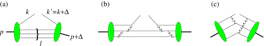
Figure 12: (a) Momenta of nucleon, active quark and spectator system in a GPD. (b) Perturbative mechanism for large $x$. (c) Hard-scattering mechanism [47] for large $t$.

That the struck quark in the soft region is far off-shell is the basis of a perturbative analysis, which has long ago been given for the $x\to 1$ limit of parton distributions or deeply inelastic structure functions (see e.g. [45]) and recently also for the $x\to 1$ limit of GPDs at arbitrary fixed $t$ [46]. It is based on graphs as the one shown in Fig. 12b, where a configuration of three quarks with momentum fractions of order $\frac{1}{3}$ and virtualities of order $\Lambda^{2}$ turns into a configuration with a fast off-shell quark and two soft quarks by successive emission of gluons, which need to be off-shell too. Standard perturbative power counting for these graphs in the momentum region just stated gives a behavior $H_{v}^{q}(x,t)\sim(1-x)^{3}$ for $x\to 1$. Their actual calculation in perturbation theory leads however to severe divergences ${\rm d}\mbox{\boldmath{$l$}}^{2}/\mbox{\boldmath{$l$}}^{4}$ in the infrared unless the quark mass is kept finite, which indicates that standard hard-scattering factorization [47] does not provide an adequate separation of short-and long-distance physics for the mechanism represented by the graphs. While the general power-counting argument might still give the correct answer, further details such as the overall normalization are currently beyond theoretical control. Resummation of radiative corrections into Sudakov form factors can give a stronger suppression than the power-law $(1-x)^{3}$ obtained from fixed-order graphs, but given the above difficulties the detailed form of these corrections (let alone their quantitative impact) is unknown. We recall that the single logarithms resummed by DGLAP evolution also modify the power of $(1-x)$, see e.g. [48].

Phenomenologically, the limiting behavior of parton densities for $x\to 1$ is poorly known. Their extraction from hard processes is increasingly difficult in this limit due to higher-twist contributions, and leading-twist analyses can use data only for values of $x$ where such contributions are under control. It is then difficult to infer a power behavior for $x\to 1$, as our attempt to extract the large-$x$ asymptotics of the profile function in Sect. 3.2 has taught us. The powers $(1-x)^{\beta}$ appearing in many parameterizations of parton densities are to be seen as parameters describing the approximate behavior of these functions over a certain range of large $x$. The CTEQ6M distributions we use in our analysis have powers $\beta_{u}\approx 2.9$ for $u_{v}$ and $\beta_{d}\approx 5.0$ for $d_{v}$ in the parameterization at the starting scale $\mu=1.3\,{\rm GeV}$. We find that at $\mu=2\,{\rm GeV}$ these distributions are described by $u_{v}(x)\sim(1-x)^{3.4}$ and $d_{v}(x)\sim(1-x)^{5.0}$ within 5% for $0.5\leq x\leq 0.9$. Taking different $x$-intervals, these parameters slightly change.

In form factors at large $t$ the relevant $x$-values of the corresponding GPDs are selected by the dynamics. Demanding $k^{2}$ and $k^{\prime 2}$ to be of the same order, the soft and ultrasoft regions are identified as

$$\begin{array}[b]{llll}\textit{soft region:}&1-x\sim\Lambda\,/\sqrt{|t|},&|k^{2}|,|k^{\prime 2}|\sim\Lambda\sqrt{|t|},&l^{+},l^{-},\mbox{\boldmath{$l$}}_{\perp}\sim\Lambda,\\[3.99994pt] \textit{ultrasoft region:}&1-x\sim\Lambda^{2}/\,|t|,&|k^{2}|,|k^{\prime 2}|\sim\Lambda^{2},&l^{+},l^{-},\mbox{\boldmath{$l$}}_{\perp}\sim\Lambda^{2}/\sqrt{|t|}.\end{array}$$

The contribution from the soft region has been analyzed in perturbation theory in the same way as for parton distributions [47, 45]. Power counting for the graph in Fig. 12b gives $F_{1}(t)\sim t^{-2}$. This is the same power as obtained with the standard hard-scattering mechanism shown in Fig. 12c, where parton virtualities are of order $|t|$. Again one may expect a further damping in the soft region by Sudakov corrections, leaving the hard-scattering mechanism as the dominant contribution at asymptotically large $-t$.

Let us now investigate the large-$t$ behavior of the form factors obtained with our parameterizations of GPDs. We see in Fig. 2 that at large $t$ the dominant contribution to $F_{1}^{p}$ comes from a rather narrow region of large $x$. To simplify the analysis we take the large-$x$ approximations $q_{v}(x)\sim(1-x)^{\beta_{q}}$ and $f_{q}(x)\sim A_{q}(1-x)^{n}$. At sufficiently large $t$ the integral $F_{1}^{q}(t)=\int{\rm d}x\,H_{v}^{q}(x,t)$ can then be evaluated in the saddle point approximation, obtained by minimizing the exponent in $H_{v}^{q}(x,t)=\exp[\,\beta_{q}\log(1-x)+tf_{q}(x)]$ with respect to $x$. We then find

$$F_{1}^{q}(t)\sim|t|^{-(1+\beta_{q})/n}\;,\qquad\qquad 1-x_{s}=\Bigg{(}\frac{n}{\beta_{q}}\,A_{q}|t|\Bigg{)}^{-1/n},$$ (34)

where $x_{s}$ is the position of the saddle point. We see that for our default fit with $n=2$ the dominant values of $x$ in the form factor are in the soft region. As observed in [49], the power behavior in (34) with $n=2$ corresponds to the Drell-Yan relation [50] between the large-$t$ behavior of form factors and the large-$x$ behavior of deep inelastic structure functions. Indeed, the kinematical assumptions made in the work of Drell and Yan correspond to the dominance of the soft region. Putting $\beta_{q}=3$ as obtained from dimensional counting we recover the $t^{-2}$ behavior mentioned above. With the phenomenological values $\beta_{u}=3.4$ and $\beta_{d}=5.0$ for our input parton distributions at large $x$ one finds that for large $t$ the form factor $F_{1}^{u}$ obtained in our fit should fall slightly faster than $t^{-2}$, whereas $F_{1}^{d}$ should decrease much more strongly. At large $t$ both proton and neutron form factor should then be dominated by $F_{1}^{u}$. Our fit result for $F_{1}^{p}$ in Fig. 6 shows the large-$t$ behavior expected from these arguments, which means that the above approximations are indeed applicable in kinematics where there is data. We will show $F_{1}^{u}$ and $F_{1}^{d}$ separately in Sect. 6.2.

Taking $n=1$ for the large-$x$ behavior of the profile function, the dominant values of $x$ in the saddle point approximation are from the ultrasoft region and give $F_{1}^{q}(t)\sim|t|^{-1-\beta_{q}}$. Our fits to (23) and (28) give a good description of the data for $F_{1}^{p}$, which are clearly incompatible with such a strong decrease in $t$. This means that the asymptotic behavior has not yet set in at $-t\approx 30\,{\rm GeV}^{2}$ for these parameterizations of GPDs. To understand this, we notice that the approximation $f^{q}(x)\approx A_{q}(1-x)^{n}$ works rather well in the interval $0.6\leq x\leq 0.9$ for our default fit, but not so well for our fits with $n=1$. Any inaccuracy in $f_{q}(x)$ appears however exponentiated in $H_{v}^{q}$ and thus in the form factors. The validity of asymptotic expansions like (34) must hence be carefully investigated on a case-by-case basis.

To quantify how close our parameterizations are from the scaling laws in (3.5), we start with $\langle x\rangle_{t}$ defined in (25) and introduce the quantity

$$\delta_{\rm eff}(t)=t\,\frac{{\rm d}}{{\rm d}t}\,\log[1-\langle x\rangle_{t}]\,,$$ (35)

which is $\frac{1}{2}$ in the soft and $1$ in the ultrasoft region. Using the saddle point approximation for both $\int{\rm d}x\,H_{v}^{q}(x,t)$ and $\int{\rm d}x\,(1-x)H_{v}^{q}(x,t)$, one readily finds that $\delta_{\rm eff}(t)$ tends to $n^{-1}$ at asymptotic values of $t$. In Fig. 13 we show $\delta_{\rm eff}(t)$ for our default fit and find that for $-t$ above $5$ to $10\,{\rm GeV}^{2}$ the scaling of the relevant $x$ values in the form factor integral is indeed the one for the soft region. In the same figure we show

$$\Lambda_{\rm eff}(t)=[1-\langle x\rangle_{t}]\,\sqrt{|t|},$$ (36)

which according to (3.5) should be of typical hadronic size for $t$ where the soft scaling law applies. This is indeed the case for our fit. We remark that with the saddle point approximation we find $\Lambda_{\rm eff}=1.26\,{\rm GeV}$ when neglecting the $d$ quark contribution to $F_{1}^{p}$ at large $t$ and taking the parameters $A_{u}=1.22\,{\rm GeV}^{-2}$ and $\beta_{u}=3.4$ for $u$ quarks. This shows once more the relevance of asymptotic considerations for our default fit in kinematics where data is available.

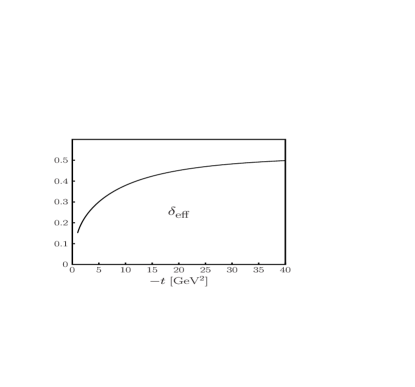
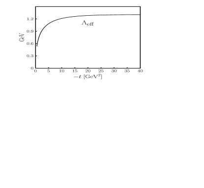
Figure 13: Dynamical interpretation of our default fit. Left: The effective power $\delta_{\rm eff}$, which describes the scaling of $(1-x)$ as a function of $|t|$. Right: The effective soft scale $\Lambda_{\rm eff}$ as a function of $|t|$.

The values of $\delta_{\rm eff}$ for our fit to (28), where $n=1$, differ from those shown in Fig. 13 by at most 8% and the values of $\Lambda_{\rm eff}$ by at most 4%. In the large-$t$ region of present data the soft contribution hence also dominates for this fit, where we find that ultrasoft behavior with $\delta_{\rm eff}=1$ only sets in for $|t|$ well above $100\,{\rm GeV}^{2}$. We remark that in our previous work [5] we used GPDs obtained from Gaussian wave functions (14), which had a profile function decreasing like $(1-x)$ at large $x$ and gave an asymptotic behavior $F_{1}(t)\sim t^{-4}$. The power counting for the “soft overlap mechanism” we set up in that work corresponds to the ultrasoft region in the parlance of our present paper. The considerations of this section make it clear that this (physically suspect) region is not the dominant one in the kinematics where the model of [5] has been used for phenomenology.

We conclude that the description of $F_{1}^{p}$ provided by our fitted GPDs supports the hypothesis that for $-t$ from about $5\,{\rm GeV}^{2}$ to several $10\,{\rm GeV}^{2}$ the dynamics is dominated by the Feynman mechanism in the soft kinematics specified above. We emphasize that by itself our result cannot exclude the dominance of the standard hard-scattering mechanism at large $t$. Applied to GPDs [51] this mechanism results in a behavior

$$H_{v}^{q}(x,t)\sim t^{-2}h(x)\qquad\qquad\mbox{for $-t\to\infty$ at fixed $x$}$$ (37)

up to logarithms in $t$. The function $h(x)$ diverges for $x\to 1$, signaling the breakdown of the factorization scheme in that limit, see [52]. Our parameterization (11) does not tend to the factorized form (37) in the large-$t$ limit and thus does not incorporate the physics of the hard-scattering mechanism. The dominance of this mechanism in $F_{1}^{p}$ at experimentally accessible $t$ is very doubtful: to be close to the data one requires proton distribution amplitudes for which a substantial fraction of the form factor comes from configurations where partons are soft and the approximations of leading-twist hard-scattering factorization are inadequate. References can e.g. be found in Sect. 10 of [19]. In our present work we make the assumption that in the $t$ region we consider, the hard-scattering mechanism is not dominant and that the Feynman mechanism controls form factors at large $t$, despite its possible Sudakov suppression in the asymptotic limit.

3.6 The $t$ dependence

In this subsection we explore an ansatz for the $t$ dependence of $H_{v}^{q}$ that is different from the exponential form we have used so far. To cover a range of possibilities we take

$$H_{v}^{q}(x,t)=q_{v}(x)\Bigg{(}1-\frac{tf_{q}(x)}{p}\Bigg{)}^{-p},$$ (38)

with different powers $p$. In the limit $p\to\infty$ we recover the exponential (11). The corresponding impact parameter distribution $q_{v}(x,\mbox{\boldmath{$b$}}^{2})$ can be expressed in terms of the modified Bessel function $K_{p-1}$ and satisfies positivity. At fixed $x$ the form (38) gives a power-law falloff $H_{v}^{q}(x,t)\sim|t|^{-p}$ for $|t|\to\infty$.

Before proceeding to fits let us investigate some general properties of this ansatz. For $p\neq 1$ the form (38) is not stable under DGLAP evolution. To see this we observe that it satisfies

$$\Bigg{(}\frac{\partial^{2}}{\partial t^{2}}\log H_{v}^{q}(x,t)\Bigg{)}\Bigg{(}\frac{\partial}{\partial t}\log H_{v}^{q}(x,t)\Bigg{)}^{-2}=\frac{1}{p}$$ (39)

for all $x$ and $t$, and starting from (7) calculate the evolution of the left-hand-side of this relation. If at a given scale $\mu$ the GPD satisfies (39) then this evolution equation simplifies to

$$\mu^{2}\frac{{\rm d}}{{\rm d}\mu^{2}}\,\Bigg{[}\Bigg{(}\frac{\partial^{2}}{\partial t^{2}}\log H_{v}^{q}(x)\Bigg{)}\Bigg{(}\frac{\partial}{\partial t}\log H_{v}^{q}(x)\Bigg{)}^{-2}\,\Bigg{]}=\Bigg{(}1-\frac{1}{p}\Bigg{)}\Bigg{(}\frac{\partial}{\partial t}\log H_{v}^{q}(x)\Bigg{)}^{-2}$$ (40)

$${}\times\int_{x}^{1}\frac{{\rm d}z}{z}\,P\Big{(}\frac{x}{z}\Big{)}\,\frac{H_{v}^{q}(z)}{H_{v}^{q}(x)}\Bigg{(}\frac{\partial}{\partial t}\log H_{v}^{q}(z)-\frac{\partial}{\partial t}\log H_{v}^{q}(x)\Bigg{)}^{2},$$

where for better legibility we have omitted the arguments $t$ and $\mu$ in the GPDs. Except for trivial functions $H_{v}^{q}(x)$ the right-hand-side of this expression is positive and furthermore depends on $x$, so that relation (39) is destroyed by evolution.

At very large $t$ the form factors obtained with (38) are again dominated by large $x$ provided that $pn>\beta_{q}$, where as before we assume the large-$x$ behaviors $q_{v}(x)\sim(1-x)^{\beta_{q}}$ and $f_{q}(x)\approx A_{q}(1-x)^{n}$. For $u$ quarks and $n=2$ this condition is fulfilled even when $p=2$. One can then again use the saddle point approximation and finds

$$F_{1}^{q}(t)\sim|t|^{-(1+\beta_{q})/n},\qquad\qquad 1-x_{s}=\Bigg{(}\Big{(}\frac{n}{\beta_{q}}\,-\frac{1}{p}\Big{)}A_{q}|t|\Bigg{)}^{-1/n},$$ (41)

where remarkably the large-$t$ behavior of $F_{1}^{q}$ is independent of $p$. The dominant $x$ in the form factor integral are in the region of the soft Feynman mechanism discussed in the previous subsection. Note that in this region $tf_{q}(x)$ is of order 1, so that the approximation giving a power-law $H_{v}^{q}(x,t)\sim|t|^{-p}$ is not valid.

We note that the form (38) does not have the Regge behavior (10) at small $x$ and $t$. Depending on $p$, this can be significant in kinematics appropriate for Regge phenomenology. Taking for example $x=10^{-3}$ and $-t=0.4\,{\rm GeV}^{2}$, we have $tf(x)\approx\alpha^{\prime}t\log(1/x)\approx-2.5$ with $\alpha^{\prime}=0.9\,{\rm GeV}^{-2}$, and $(1+2.5/p)^{-p}$ is about twice as large as $\exp(-2.5)$ if $p=3$. Having lost the connection with Regge phenomenology, we will not impose a fixed value of $\alpha^{\prime}$ in our fits. A logarithmic increase of $\langle\mbox{\boldmath{$b$}}^{2}\rangle_{x}$ at small $x$ seems however plausible from a more general point of view, and we keep the analytic form of our profile function as in our default fit. One could of course construct parameterizations which interpolate between an exponential $t$ dependence at very small $x$ and a power-law when $x$ becomes larger. Since the small-$x$ region does however not affect our fit to nucleon form factors for $-t$ above $1\,{\rm GeV}^{2}$ or so, we shall not pursue this possibility here.

The results of our fits to (38) and (29) are shown in Table 11 for selected values of $p$, where for easier comparison we have also given the result of our exponential fit with free $\alpha^{\prime}$ discussed in Sect. 3.4. As $p$ decreases from $\infty$, the quality of the fit first improves (except for the neutron data). The smallest $\chi^{2}$ is attained for $p=2.5$, and further decrease of $p$ makes the fit worse. With $p=2$ no good description of the large-$t$ data can be achieved: the fit result for $F_{1}^{p}$ systematically overshoots the data above $-t=9\,{\rm GeV}^{2}$, by about $15\%$ when $-t>19\,{\rm GeV}^{2}$. We find the same qualitative picture when fixing $\alpha^{\prime}=0.9\,{\rm GeV}^{-2}$ in the fit. The lowest $\chi^{2}$ is then obtained at $p=3$, and for $p=2$ the description of the large-$t$ data is again very bad. It is important to realize that, despite a clear decrease in $\chi^{2}$, the description of the data for $F_{1}^{p}$ does not improve dramatically when going from $p=\infty$ to $p=2.5$. Except for the two data points with the largest values of $-t$ and the data point with $-t=0.86\,{\rm GeV}^{2}$ (which has the highest $-t$ in the sample of [41]), the pull for $F_{1}^{p}$ of our fit with $p=2.5$ is at most $3\%$ in magnitude, whereas it is at most $3.5\%$ with our default fit.

With decreasing $p$ the profile functions $f_{q}(x)$ increase significantly, which is shown in Fig. 14 for $u$ quarks. This can be readily understood: the GPDs in (38) decrease much smaller in the variable $|t|f_{q}(x)$ for small $p$ than for large $p$, so that small $p$ requires a larger $f_{q}(x)$ in order to not overshoot the form factors at large $|t|$.

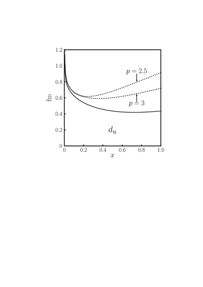
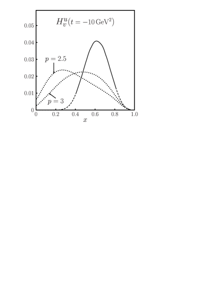
Figure 14: Left: The distance $d_{u}(x)$ between struck quark and spectators obtained with fits to the power-law (38) with $p=2.5$ and $p=3$, compared with the result of our default fit, which corresponds to $p\to\infty$ and differs only slightly from the corresponding fit with free $\alpha^{\prime}$. Right: The results for $H_{v}^{u}(x,t)$ at $-t=10\,{\rm GeV}^{2}$ from the same fits.

In the figure we also show the $x$ dependence of $H_{v}^{u}$ at large $t$. Its shape is much broader for the fits with smaller $p$ and reaches down to smaller $x$. This reflects that when $p$ becomes smaller it takes significantly larger $t$ to suppress $H_{v}^{q}$ at a given $x$. For small $p$ the asymptotic behavior (41) obtained with the saddle-point approximation should hence set in at much larger $t$. Taking $-t=40\,{\rm GeV}^{2}$ we find indeed that $\langle x\rangle_{t}$ is only 0.6 for $p=3$ and 0.5 for $p=2.5$, and that $\delta_{\rm eff}$ only becomes 0.3 for $p=3$ and 0.15 for $p=2.5$, to be compared with the corresponding values $\langle x\rangle_{t}=0.8$ and $\delta_{\rm eff}=0.5$ for the default fit.

As is seen in Fig. 14, the GPDs with power-law form (38) do not vanish for $x\to 0$ at large $t$, so that small $x$ also contribute in the high-$t$ form factors to some extent. This is in contrast to the GPDs with exponential $t$ dependence. Using that $q_{v}(x)\sim x^{-\alpha}$ for $x\to 0$, one readily finds that $H_{v}^{q}(x,t)\sim x^{-\alpha-\alpha^{\prime}t}$ vanishes in this limit as soon as $-t\raisebox{-4.0pt}{$\,\stackrel{{\scriptstyle\textstyle>}}{{\sim}}\,$}\alpha/\alpha^{\prime}$, i.e., already for $-t$ above $0.7\,{\rm GeV}^{2}$ or so.

The fits we have shown make it clear that a significant ambiguity remains when one tries to determine the correlated dependence on $x$ and $t$ of GPDs from experimental knowledge of their integrals over $x$ and of their limits at $t=0$. Without data on observables depending on both variables we need a certain theoretical bias in our extraction of GPDs. We regard the connection of our default fit with Regge phenomenology at small $x$ and $t$ and with the dynamics of the soft Feynman mechanism at large $t$ as physically attractive features and retain the exponential form (11) for the $t$ dependence of $H_{v}^{q}(x,t)$.

4 The polarized distribution $\widetilde{H}_{v}(x,t)$

In this section we investigate the distribution of polarized quarks and its connection with the isovector axial form factor $F_{A}(t)$ of the nucleon. The relevant sum rule reads

$$F_{A}(t)=\int_{-1}^{1}{\rm d}x\,\Big{(}\widetilde{H}^{u}(x,t,\mu^{2})-\widetilde{H}^{d}(x,t,\mu^{2})\Big{)}.$$ (42)

Its value at $t=0$ is given by the axial charge $F_{A}(0)$ and well known from $\beta$ decay experiments. The measurement of $F_{A}(t)$ covering the largest $t$ range [53] has been performed in charged current scattering $\nu_{\mu}\,n\to\mu^{-}p$. The result has been given in the form of a dipole parameterization

$$F_{A}(t)=\frac{F_{A}(0)}{(1-t/M_{A}^{2})^{2}_{\phantom{A}}}$$ (43)

with $F_{A}(0)=1.23\pm 0.01$ and $M_{A}=(1.05\,^{+0.12}_{-0.16})\,{\rm GeV}$ for a measured range $0.1\,{\rm GeV}^{2}\leq-t\leq 3\,{\rm GeV}^{2}$. The resulting $t$ dependence of $F_{A}(t)$ is not too different from the one of the proton Dirac form factor: we find that $F_{1}^{p}(t)$ can be approximated to 9% accuracy for $-t\leq 3\,{\rm GeV}^{2}$ by $(1-t/M_{D}^{2})^{-2}$ with $M_{D}=0.98\,{\rm GeV}$. Note that the well-known dipole mass of $0.84\,{\rm GeV}$ does not refer to $F_{1}^{p}$ but to a dipole parameterization of the magnetic form factors of proton and neutron, $G_{M}^{p}$ and $G_{M}^{n}$.

Many other measurements of $F_{A}(t)$ in either charged current scattering or $ep\to e\pi^{+}n$ have also been presented in terms of a dipole mass, with a considerable spread of results for $-t\leq 1\,{\rm GeV}^{2}$ (see e.g. [54]). We remark that while a dipole form (43) provides a simple and compact parameterization, it is not well suited for a description of data beyond a certain accuracy. It is instructive in this respect to perform dipole fits to the data on $F_{1}^{p}$ or on $G_{M}^{p}$ in different ranges of $t$ and to observe the shift in the dipole mass.

Given the data situation for $F_{A}(t)$ we do not attempt a fit of GPDs to the sum rule (42), but rather test the simple ansatz

$$\widetilde{H}^{q}_{v}(x,t)=\Delta q_{v}(x)\,\exp{[t\tilde{f}_{q}(x)]}$$ (44)

with the profile functions $\tilde{f}_{q}(x)$ taken equal to $f_{q}(x)$ obtained in our default fit for the unpolarized distributions $H_{v}^{q}$. In physical terms this ansatz assumes that the distribution of quarks minus antiquarks in the transverse plane does not depend on the quark or antiquark helicity relative to the helicity of the proton. For our evaluation we take the polarized parton densities $\Delta q_{v}(x)$ from [21], more specifically the NLO distributions in their scenario 1 at $\mu=2\,{\rm GeV}$.

Since the axial form factor has positive charge parity, it is not directly connected with the valence quark distributions. Instead we have

$$F_{A}(t)=\int_{0}^{1}{\rm d}x\,\Big{(}\widetilde{H}_{v}^{u}(x,t)-\widetilde{H}_{v}^{d}(x,t)\Big{)}+2\int_{0}^{1}{\rm d}x\,\Big{(}\widetilde{H}^{\bar{u}}(x,t)-\widetilde{H}^{\bar{d}}(x,t)\Big{)},$$ (45)

where the generalized antiquark distributions are given by $\widetilde{H}^{\bar{q}}(x,t)=\widetilde{H}^{q}(-x,t)$. The flavor nonsinglet combination $\Delta\bar{u}(x)-\Delta\bar{d}(x)$ of forward densities is poorly known, and at present there is no experimental evidence that it might be large [55]. To make a motivated ansatz for its analog at finite $t$ is beyond the scope of this work. For a very crude estimate we have taken $\widetilde{H}^{\bar{q}}(x,t)=\Delta\bar{q}(x)\exp[tf_{q}(x)]$ with the polarized antiquark distributions from [21], where $\Delta\bar{u}(x)=\Delta\bar{d}(x)$. The resulting contribution from antiquark GPDs in (45) is below a percent, both for $f_{q}(x)$ from our default fit and from the corresponding four-parameter fit in Table 8, where $B_{u}\neq B_{d}$, This is because the profile functions for $u$ and $d$ quarks differ mostly at larger $x$, where antiquarks do not abound.

The present uncertainties on polarized quark distributions are significantly larger than those on their unpolarized counterparts. We have calculated the resulting error on $F_{A}(t)$ using the covariance matrix on the parameters in the parton densities provided in [21]. This error is at least a factor of 5 larger than the error resulting from the uncertainty in $f_{q}(x)$. For estimating the parametric uncertainties of $F_{A}(t)$ obtained with our ansatz, we have added the errors from the two sources in quadrature.

In Fig. 15 we show the contribution to $F_{A}(t)$ from the valence quark GPDs specified above. We compare this with the dipole parameterization of [53], which we have extrapolated up to $-t=5\,{\rm GeV}^{2}$. Our result undershoots the central value of that parameterization by at most 13%, with the largest discrepancy for $-t$ between $0.5$ and $1\,{\rm GeV}^{2}$. It is however consistent within the errors of the parameterization in the full range $0.1\,{\rm GeV}^{2}\leq-t\leq 3\,{\rm GeV}^{2}$ of the measurement in [53]. We note that one obtains a larger form factor with the ansatz (44) when taking a smaller profile function $\tilde{f}_{q}(x)$. This is indeed physically allowed, whereas taking $\tilde{f}_{q}(x)>f_{q}(x)$ would violate the positivity of parton densities in impact parameter space (see Sect. 5.2).

Figure 15: Axial form factor $F_{A}(t)$ obtained from the valence distributions (44) with polarized densities from [21] at $\mu=2\,{\rm GeV}^{2}$ and the result of our default fit for $f_{q}(x)$ specified in Sect. 3.2. The contribution from sea quarks has been neglected. The error band gives the $1\,\sigma$ uncertainties of the fit to $f_{q}(x)$ added in quadrature to those of $\Delta q(x)$. The curve and band shown up to $-t=5\,{\rm GeV}^{2}$ represents the dipole parameterization from [53] with $F_{A}(0)=1.23\pm 0.01$ and $M_{A}=(1.05\,^{+0.12}_{-0.16})\,{\rm GeV}$.

In conclusion, we find that the present data on the axial form factor is consistent with valence quark dominance in the sum rule (45) and with only a weak helicity dependence in the transverse distribution of valence quarks at not too large values of $x$. We note that $x_{\rm max}(t)$ for $F_{A}(t)$, defined in analogy to (24), equals $0.73$ at $-t=3\,{\rm GeV}^{2}$.

5 The helicity-flip distribution $E$ from the Pauli form factors

5.1 General properties

The GPDs $E^{q}$ are related to the Pauli form factors of proton and neutron through the sum rules

$$F^{p}_{2}(t) = \int_{0}^{1}{\rm d}x\,\Big{[}{\textstyle\frac{2}{3}}E_{v}^{u}(x,t,\mu^{2})-{\textstyle\frac{1}{3}}E_{v}^{d}(x,t,\mu)\Big{]}\,,$$

$$F^{n}_{2}(t) = \int_{0}^{1}{\rm d}x\,\Big{[}{\textstyle\frac{2}{3}}E_{v}^{d}(x,t,\mu^{2})-{\textstyle\frac{1}{3}}E_{v}^{u}(x,t,\mu)\Big{]}\,,$$ (46)

where in analogy to (1) we have introduced valence distributions

$$E_{v}^{q}(x,t,\mu^{2})=E^{q}(x,t,\mu^{2})+E^{q}(-x,t,\mu^{2})$$ (47)

for quarks of flavor $q$ in the proton. Contributions from sea quarks cancel in (46). We have neglected in (46) the contribution from strange quarks, as we did for the Dirac form factors. The scale dependence of $E_{v}$ is described by the same DGLAP equation as the scale dependence of $H_{v}$, since both distributions belong to the same quark operator.

The distribution $E^{q}_{v}(x,t)$ describes proton helicity flip in a frame where the proton moves fast (or more precisely light-cone helicity flip, see e.g. Sect. 3.5 of [19]). Since quark helicity is conserved by the vector current, proton helicity flip requires orbital angular momentum between the struck quark and the spectator system. This becomes for instance manifest by writing $E^{q}_{v}$ as the overlap of light-cone wave functions, whose orbital angular momentum must differ by exactly one unit. Another manifestation is Ji’s sum rule for the combination $H^{q}(x,t)+E^{q}(x,t)$, see Section 6.3.

$E^{q}_{v}$ admits a probability interpretation in impact parameter space if one changes basis from longitudinal to transverse polarization states of the proton [24]. More precisely, one considers states of definite proton transversity, which is the light-cone analog of transverse polarization, see e.g. [56]. The distribution

$$q_{v}^{X}(x,\mbox{\boldmath{$b$}})=q_{v}(x,\mbox{\boldmath{$b$}})-\frac{b^{y}}{m}\,\frac{\partial}{\partial\mbox{\boldmath{$b$}}^{2}}\,e_{v}^{q}(x,\mbox{\boldmath{$b$}})$$ (48)

gives the probability to find an unpolarized quark with momentum fraction $x$ and impact parameter $\mbox{\boldmath{$b$}}=(b^{x},b^{y})$ in a proton polarized along the $x$ direction, minus the corresponding probability to find an antiquark. Here we have introduced the Fourier transform

$$e_{v}^{q}(x,\mbox{\boldmath{$b$}})=\int\frac{{\rm d}^{2}\mbox{\boldmath{$\Delta$}}}{(2\pi)^{2}}\,e^{-i\mbox{\boldmath{$\scriptstyle b$}}\mbox{\boldmath{$\scriptstyle\Delta$}}}\,E_{v}^{q}(x,t=-\mbox{\boldmath{$\Delta$}}^{2}).$$ (49)

Note that $e_{v}^{q}(x,\mbox{\boldmath{$b$}})$ and $q_{v}(x,\mbox{\boldmath{$b$}})$ depend on $b^{x}$ and $b^{y}$ only via $\mbox{\boldmath{$b$}}^{2}$. We see from (48) that target polarization along the $x$-axis induces a shift in the quark distribution along the $y$-axis. As explained in [24], this effect is consistent with the classical picture of the polarized proton as a sphere rotating about the $x$-axis and moving in the $z$-direction (see also [57]). The average displacement of this shift is

$$\langle b^{y}\rangle^{q}_{x}=\frac{\int{\rm d}^{2}\mbox{\boldmath{$b$}}\;b^{y}\,q_{v}^{X}(x,\mbox{\boldmath{$b$}})}{\int{\rm d}^{2}\mbox{\boldmath{$b$}}\,q_{v}^{X}(x,\mbox{\boldmath{$b$}})}=\frac{1}{2m}\,\frac{E_{v}^{q}(x,0)}{H_{v}^{q}(x,0)}\,,$$ (50)

and its scale evolution is given by

$$\mu^{2}\frac{{\rm d}}{{\rm d}\mu^{2}}\langle b^{y}\rangle^{q}_{x}=-\frac{1}{q_{v}(x)}\int_{x}^{1}\frac{{\rm d}z}{z}\,P\Big{(}\frac{x}{z}\Big{)}\,q_{v}(z)\Big{[}\langle b^{q}\rangle^{q}_{x}-\langle b^{q}\rangle^{q}_{z}\Big{]},$$ (51)

in analogy to the evolution of $\langle\mbox{\boldmath{$b$}}^{2}\rangle^{q}_{x}$. The corresponding shift for the distance between the struck quark and the spectator system is

$$s_{q}(x)=\frac{\langle b^{y}\rangle^{q}_{x}}{1-x},$$ (52)

in analogy to the distance function $d_{q}(x)$ we introduced in (6).

The impact parameter space distributions satisfy inequalities which insure that the quark densities for various combinations of proton and quark spins are positive. Using the methods of [58] one finds in particular [49]

$$\frac{\mbox{\boldmath{$b$}}^{2}}{m^{2}}\Bigg{(}\frac{\partial}{\partial\mbox{\boldmath{$b$}}^{2}}\,e^{q}(x,\mbox{\boldmath{$b$}})\Bigg{)}^{2}\leq\Big{[}q(x,\mbox{\boldmath{$b$}})+\Delta q(x,\mbox{\boldmath{$b$}})\Big{]}\,\Big{[}q(x,\mbox{\boldmath{$b$}})-\Delta q(x,\mbox{\boldmath{$b$}})\Big{]}\,,$$ (53)

where $e^{q}(x,\mbox{\boldmath{$b$}})$, $q(x,\mbox{\boldmath{$b$}})$ and $\Delta q(x,\mbox{\boldmath{$b$}})$ are the respective Fourier transforms of $E^{q}(x,t)$, $H^{q}(x,t)$ and $\widetilde{H}^{q}(x,t)$, defined in analogy to (3) and (49). The bound (53) is stable under leading-order DGLAP evolution to higher scales, and a closer look at its derivation shows that it should be valid when $\mu$ is large enough for the application of leading-twist factorization theorems to the exclusive processes where GPDs appear. For a discussion and references see [19].

Multiplying (53) with $\mbox{\boldmath{$b$}}^{2}$ and integrating over $b$, one obtains after a few steps an inequality for GPDs in momentum space [49],

$$\Big{(}E^{q}(x,0)\Big{)}^{2}\leq 4m^{2}\Big{[}q(x)+\Delta q(x)\Big{]}\,\Big{[}q(x)-\Delta q(x)\Big{]}\,\frac{\partial}{\partial t}\ln\left[H^{q}(x,t)\pm\tilde{H}^{q}(x,t)\right]_{t=0}\ ,$$ (54)

where either the sum or the difference of $H^{q}$ and $\widetilde{H}^{q}$ may be taken. The $t$-derivative on the right-hand side is $\frac{1}{4}$ times the average squared impact parameter of quarks with positive or negative helicity. According to our discussion in Sect. 3.1 this quantity may be expected to decrease at least like $(1-x)^{2}$ in the limit $x\to 1$. Since in addition the longitudinal polarization $|\Delta q/q|$ of quarks is phenomenologically seen to grow as $x$ becomes large, the inequality (54) severely limits the high-$x$ behavior of $E^{q}(x,t=0)$ and will be an essential input in the following.

The positivity constraints (53) and (54) hold for the distribution of quarks (i.e. for $x>0$) and have analogs for antiquarks. They do not hold for the valence combinations we aim to determine in this work, which are differences of quark and antiquark distributions. It is however natural to neglect antiquarks at large enough $x$, which is in fact the region where the bounds give the strongest constraints. With this proviso in mind we will in the following use (53) and (54) for the valence distributions.

Our discussion of the bound (54) implies that the average displacement $\langle b^{y}\rangle^{q}_{x}$ should vanish in the limit of $x\to 1$. At large enough $x$ it should hence be a decreasing function, which according to (51) implies that $\langle b^{y}\rangle^{q}_{x}$ becomes smaller when evolving to higher scales $\mu$. We comment on the small-$x$ behavior of this displacement in the next subsection.

5.2 Ansatz for $E_{v}(x,t)$

Our ansatz for $E_{v}$ is taken in analogy to the other GPDs as

$$E_{v}^{q}(x,t)=e_{v}^{q}(x)\,\exp[tg_{q}(x)],$$ (55)

where we use the notation

$$e_{v}^{q}(x)=E_{v}^{q}(x,t=0)$$ (56)

for the forward limit. The normalization integrals

$$\int_{0}^{1}{\rm d}x\,e_{v}^{q}(x,t=0,\mu)=\kappa_{q}$$ (57)

give the contribution of quark flavor $q$ to the anomalous magnetic moment of the proton (up to quark charge factors). Neglecting the contribution from strange quarks one has according to (46)

$$\kappa_{u}=2\kappa_{p}+\kappa_{n}\approx 1.67\,,\qquad\qquad\kappa_{d}=\kappa_{p}+2\kappa_{n}\approx-2.03\,.$$ (58)

For the profile function in (55) we take the same form as in our default fit for $H_{v}^{q}$,

$$g_{q}(x)=\alpha^{\prime}(1-x)^{3}\log\frac{1}{x}+D_{q}(1-x)^{3}+C_{q}\,x(1-x)^{2}\hskip 40.00006pt\mbox{with~{}}\alpha^{\prime}=0.9\,{\rm GeV}^{-2}\>.$$ (59)

The motivation from Regge phenomenology for the behavior of $g_{q}$ at very small $x$ applies in the same way as for $f_{q}$. Indeed the Regge exchanges contributing to $H_{v}^{q}$ and $E_{v}^{q}$ are the same, and only their coupling strengths differ. We therefore take the same fixed value of $\alpha^{\prime}$ as in our default fit for $H_{v}^{q}$.

The exponential $t$-dependence for $\widetilde{H}_{v}^{q}$ and $E_{v}^{q}$ taken in (44) and (55) gives

$$\Delta{q}_{v}(x,\mbox{\boldmath{$b$}})=\frac{1}{4\pi}\,\frac{\Delta q_{v}(x)}{\tilde{f}_{q}(x)}\,\exp\Bigg{[}-\frac{\mbox{\boldmath{$b$}}^{2}}{4\tilde{f}_{q}(x)}\Bigg{]}\>,\qquad\qquad e_{v}(x,\mbox{\boldmath{$b$}})=\frac{1}{4\pi}\,\frac{e_{v}(x)}{g_{q}(x)}\,\exp\Bigg{[}-\frac{\mbox{\boldmath{$b$}}^{2}}{4g_{q}(x)}\Bigg{]}$$ (60)

in analogy to the form (12) of $q_{v}(x,\mbox{\boldmath{$b$}})$. According to (53) one must have $|\Delta q_{v}(x,\mbox{\boldmath{$b$}}|\leq q_{v}(x,\mbox{\boldmath{$b$}})$ for all $b$ when antiquarks are negligible, which implies $\tilde{f}_{q}(x)\leq f_{q}(x)$ as anticipated in Sect. 4. With our simplified ansatz $\tilde{f}_{q}(x)=f_{q}(x)$, the bounds (53) and (54) respectively read

$$\frac{\mbox{\boldmath{$b$}}^{2}}{(4mg_{q})^{2}}\,\Bigg{(}\frac{e_{v}^{q}}{g_{q}}\Bigg{)}^{2}\exp\Bigg{[}-\frac{\mbox{\boldmath{$b$}}^{2}}{2g_{q}}\Bigg{]}\leq\frac{(q_{v})^{2}-(\Delta q_{v})^{2}}{(f_{q})^{2}}\,\exp\Bigg{[}-\frac{\mbox{\boldmath{$b$}}^{2}}{2f_{q}}\Bigg{]}$$ (61)

and

$$(e_{v}^{q})^{2}\leq 4m^{2}f_{q}\,\Big{[}(q_{v})^{2}-(\Delta q_{v})^{2}\Big{]}$$ (62)

when antiquarks can be neglected, where for the sake of legibility we have omitted the argument $x$ in all functions. Because of the factor $\mbox{\boldmath{$b$}}^{2}$ on the left-hand side of (61) we must have

$$g_{q}(x)<f_{q}(x)$$ (63)

with strict inequality, otherwise the bound will be violated at sufficiently large $\mbox{\boldmath{$b$}}^{2}$. Multiplying both sides of (61) with $\exp[\mbox{\boldmath{$b$}}^{2}/(2f_{q})]$ and then maximizing the left-hand side, one finds that the bound is most stringent for $\mbox{\boldmath{$b$}}^{2}=2g_{q}f_{q}/(f_{q}-g_{q})$, where it reads

$$(e_{v}^{q})^{2}\leq 4m^{2}\,e^{1+\log 2}\,\Bigg{(}\frac{g_{q}}{f_{q}}\Bigg{)}^{3}(f_{q}-g_{q})\,\Big{[}(q_{v})^{2}-(\Delta q_{v})^{2}\Big{]}.$$ (64)

We note that the bound (62) is weaker than (64) but has the practical advantage to be independent of the profile function $g_{q}$. If we require the distance $d_{q}(x)$ between struck quark and spectators in an unpolarized proton to stay finite in the limit $x\to 1$, then this bound guarantees that the shift $s_{q}(x)$ of this distance also remains finite, given that $e_{v}^{q}=2m\,(1-x)q_{v}\,s_{q}$ and $f_{q}=(1-x)^{2}\,d_{q}^{2}/4$.

For the shape of $e_{v}^{q}$ we make the time-honored ansatz

$$e_{v}^{q}(x)=N_{q}\kappa_{q}\,x^{-\alpha}\,(1-x)^{\beta_{q}}\,,$$ (65)

whose analog for $q_{v}$ and $\Delta q_{v}$ gives a reasonable first approximation of phenomenologically extracted parton densities. The factor

$$N_{q}=\frac{\Gamma(2-\alpha+\beta_{q})}{\Gamma(1-\alpha)\Gamma(1+\beta_{q})}$$ (66)

ensures the proper normalization (57). In the small-$x$ limit $\alpha$ takes the role of a Regge intercept if one assumes dominance of a single Regge pole, see Sect. 3.1. From Regge phenomenology and from experience with $q_{v}$ one expects $\alpha\approx 0.5$ for both $u$ and $d$ quarks. Note however that the form (65) is sensitive to $\alpha$ over a finite interval of $x$, and we do not have enough data to introduce further parameters which would make the description of $e_{v}^{q}$ more flexible. For the average displacement $\langle b^{y}\rangle^{q}_{x}$ in (50) we expect a relatively weak $x$-dependence at small $x$, say a power-law $x^{\delta}$, where $\delta$ should be of order $0.1$ but may be positive or negative. In line with our treatment of $\alpha^{\prime}$ we have taken a single parameter $\alpha$ for $u$ and $d$ quarks in all our fits. Trying to determine a flavor dependence at the level of what is seen in the distributions $q_{v}(x)$ is beyond the accuracy we can hope for in this study.

5.3 Fit to the Pauli form factors

Before proceeding to the fits of $E^{q}_{v}$ we would like to point out two features of the data on the Pauli form factors. As we saw in Sect. 3.4, a comparison of the Dirac form factors for proton and neutron clearly shows that with growing $|t|$ the ratio of $F_{1}^{d}$ and $F_{1}^{u}$ must become smaller than its value $\frac{1}{2}$ at $t=0$. Let us investigate the evolution with $|t|$ for the analogous ratio of individual flavor contributions $F_{2}^{q}(t)=\int_{0}^{1}{\rm d}x\,E_{v}^{q}(x,t)$ to the Pauli form factor. Writing $r_{2}=(\kappa_{d}^{-1}F_{2}^{d})/(\kappa_{u}^{-1}F_{2}^{u})$ we obtain

$$R_{2}=\frac{\kappa_{n}^{-1}F_{2}^{n}}{\kappa_{p}^{-1}F_{2}^{p}}\approx\frac{1+0.71\,(r_{2}-1)}{1+0.38\,(r_{2}-1)}\approx 1+0.33\,(r_{2}-1),$$ (67)

where we have inserted the values of the anomalous magnetic moments and in the last step expanded in the deviation of $r_{2}$ from its value at $t=0$. In Fig. 16 we show the normalized form factors $\kappa_{p}^{-1}F_{2}^{p}$ and $\kappa_{n}^{-1}F_{2}^{n}$, weighted with a factor $|t|$ to make the region where we have neutron data more visible. We observe that the five neutron data points with $-t$ between $0.25$ and $1.2\,{\rm GeV}^{2}$ have a tendency to be above the data for the proton. We note that these points are from three different measurements [59, 60], [61] and [62], so that this effect is at least not due to a normalization problem in a single experiment. According to (67), a positive value of $R_{2}-1$ implies a positive value of $r_{2}-1$ about three times as large, so that $\kappa_{u}^{-1}F_{2}^{u}(t)$ must decrease faster than $\kappa_{d}^{-1}F_{2}^{d}(t)$ starting from $t=0$. This is the opposite of what is found for the Dirac form factors, and it would be interesting to have better neutron data to see if this trend is confirmed, and possibly reversed at larger $t$. With the data and errors at our disposal, the trend has a clear effect on our fit of $E_{v}^{u}$ and $E_{v}^{d}$.

In Fig. 17 we show $F_{2}^{p}$ weighted with a factor $t^{2}$ (as we did for the Dirac form factors) and find a striking plateau for $-t$ between $2.5$ and $5.5\,{\rm GeV}^{2}$. A behavior $F_{2}^{p}\sim t^{-2}$ is certainly not expected in the large-$t$ limit. The plot in Fig. 17 thus instructs us that observables may exhibit an approximate power-law behavior in an intermediate range of a kinematical variable, which has little to do with the asymptotic behavior.

Figure 16: Data for the normalized form factors $\kappa_{p}^{-1}F_{2}^{p}$ and $\kappa_{n}^{-1}F_{2}^{n}$ weighted with $|t|$.

Figure 17: Data for the weighted form factor $t^{2}F_{2}^{p}(t)$. Full symbols: results obtained with the recoil polarization method [88, 76, 89]. Open symbols: results from the Rosenbluth separation in [90].

Apart from their connection with the Pauli form factors, we have at present no phenomenological constraints on the shape of the GPDs $E^{q}(x,\xi,t)$. With data for $F_{2}$ going up to $-t=5.5\,{\rm GeV}^{2}$ for the proton and even less for the neutron, we must expect that a significant range of functions $e_{v}^{q}(x)$ and $g_{q}(x)$ in (55) is able to describe the form factors. In particular, the fit can partially accommodate a decreased value of $\beta_{q}$ by simultaneously increasing $g_{q}$, thus partially compensating a shift of $e_{v}^{q}(x)$ to larger values of $x$ by a stronger suppression through the exponential factor $\exp[tg_{q}(x)]$ in that region of $x$. The bounds (62) and (63) provide lower limits on $\beta_{q}$ and upper limits on $g_{q}(x)$. In the opposite direction we have only the requirement that $g_{q}(x)$ must be positive for the exponential ansatz (55) to make sense.

Performing fits to the data on $F_{2}^{p}$ and $F_{2}^{n}$ where the parameters $C_{u}$ and $C_{d}$ are left free, we find that the values of $C_{d}$ and (depending on the details of the fit) also of $C_{u}$ are too large to fulfill the bound (63), which results in an exponentially strong violation of (61) for large enough $x$ and $\mbox{\boldmath{$b$}}^{2}$. We have therefore in the minimum-$\chi^{2}$ fits imposed the bounds

$$C_{u}\leq A_{u}=1.22\,{\rm GeV}^{-2},\qquad\qquad C_{d}\leq A_{d}=2.59\,{\rm GeV}^{-2}.$$ (68)

The values of $A_{u}$ and $A_{d}$ in (68) are those obtained in our default fit to the Dirac form factors (see Sect. 3.2). Directly implementing (62) or (64) in the fit would be more involved, and we have instead verified these bounds only for the fit results. We remark that with our input parton densities at $\mu=2\,{\rm GeV}$ (CTEQ6M [20] and the NLO distributions in scenario 1 of [21]) the inequalities $|\Delta q(x)|\leq q(x)$ and $|\Delta q_{v}(x)|\leq q_{v}(x)$ are violated for the best fit values of the distributions at $x$ above 0.6 or 0.7, but are well satisfied within the $1\,\sigma$ error bands on the polarized densities from [21]. We therefore require the bounds (61), (62), (64) to hold within these errors.

Notice that when fitting $E_{v}^{q}(x,t,\mu^{2})$ to the Pauli form factors alone, we cannot determine the scale $\mu$ since the form factor integrals in (46) are scale independent. We fix $\mu$ implicitly in our fit by requiring the positivity condition (64) to hold for the parton densities at $\mu=2\,{\rm GeV}$ and the associated profile function $f_{q}(x)$ obtained in our default fit of $H_{v}^{q}$.

To avoid dealing with too many free parameters, we will present fits where we imposed $\alpha=0.55$. Leaving $\alpha$ free in those fits which give a good description of the data, we obtain values between $0.5$ and $0.6$. Following the discussion at the end of the previous subsection, this validates once more our assumption that simple Regge phenomenology provides a guide for the behavior of GPDs at small $x$ and small $t$. For those fits which fail to describe the data, making $\alpha$ a free parameter does not help. The conclusions we draw in the following are hence not affected by having fixed the parameter $\alpha$.

Even then we still have six parameters to determine, namely $\beta_{q}$, $C_{q}$ and $D_{q}$ for each quark flavor. To gain some insight into the range of allowed parameters, we have performed a series of fits with fixed values of $\beta_{u}$ and $\beta_{d}$, leaving the other four parameters to be fitted. The resulting values of $\chi^{2}/\mathrm{d.o.f.}$ are shown in Table 1 and the results for a subset of these fits in Table 12. Distributions with $\beta_{u}=3$ or with $\beta_{d}=4$ violate the positivity condition (62) at large $x$ and have been discarded. A number of observations can be made in these fits:

1. Both $C_{q}$ and $D_{q}$ increase when $\beta_{u}$ decreases, and for $\beta_{u}=4$ the fit selects the maximum allowed value $C_{u}=A_{u}$. For all fits shown in Table 1 the fit selects the maximum $C_{d}=A_{d}$, and only $D_{d}$ increases when $\beta_{d}$ becomes smaller.

2. The minimum $\chi^{2}$ is very flat as a function of $\beta_{u}$ and even more of $\beta_{d}$. In particular there is only a slight preference to have $\beta_{u}<\beta_{d}$, with good fits being also obtained for $\beta_{u}\geq\beta_{d}$.

3. The fitted parameters $D_{u}$ and $D_{d}$ differ significantly within their errors—much more strongly than in our our fits to the Dirac form factors (see Sect. 3.4).

Table 1: Values of $\chi^{2}/\mathrm{d.o.f.}$ obtained in fits to (55), (59) and (65) with fixed $\alpha=0.55$. Free parameters are $D_{u}$, $D_{d}$ and $C_{u}$, $C_{d}$ under the constraints (68).

	$\beta_{u}$
	4	5	6	7
$\beta_{d}$	$\chi^{2}/\mathrm{d.o.f.}$
5	1.32	1.36	1.41	1.47
6	1.31	1.36	1.41	1.47
7	1.33	1.37	1.42	1.48
8	1.36	1.39	1.44	1.50
9	1.44	1.42	1.47	1.52

These fits with a grid of fixed values $\beta_{u}$ and $\beta_{d}$ are not well suited for the propagation of correlated errors. We have thus performed a six-parameter fit with free $\beta_{u}$, $\beta_{d}$, $C_{u}$, $C_{d}$, $D_{u}$ and $D_{d}$, fixing only $\alpha=0.55$. The minimum $\chi^{2}$ is achieved for $\beta_{u}=3.99$ and $\beta_{d}=5.59$, and the parameters $C_{u}$ and $C_{d}$ take their maximum values given in (68). To avoid the treatment of errors on parameters at the boundary of their allowed range, we have fixed their values to $C_{u}=1.22\,{\rm GeV}^{-2}$ and $C_{d}=2.59\,{\rm GeV}^{-2}$ and repeated the fit. The resulting four-parameter fit still has a very large error of $2.67$ on $\beta_{d}$. In addition, this error is strongly correlated with the error on $D_{d}$, with a linear combination of the two parameters being essentially undetermined. The available data on the Pauli form factors do not allow us to extract four independent parameters within an acceptable accuracy. As a simple solution one might impose the constraint $\beta_{u}=\beta_{d}$, but this results in a fitted value of $\beta_{q}=4.21$, which is in clear violation of the positivity bound (62). As an alternative we have fixed the difference $\beta_{d}-\beta_{u}$ to the value $1.6$ obtained in the six- and four-parameter fits just discussed. This value is then to be regarded as an external input to a three-parameter fit with

$$\begin{array}[b]{llll}\beta_{u}&=\,3.99\pm 0.22,&\beta_{d}&=\,\beta_{u}+1.60,\\ C_{u}&=\,1.22\,{\rm GeV}^{-2},&C_{d}&=\,2.59\,{\rm GeV}^{-2},\\ D_{u}&=\,(0.38\pm 0.11)\,{\rm GeV}^{-2},{}{}{}{}{}{}&D_{d}&=\,-(0.75\pm 0.05)\,{\rm GeV}^{-2},\end{array}$$ (69)

and $\alpha=0.55$. Full details are given in App. B. We take this as our default fit for $E_{v}^{q}$ in the rest of this paper. We remark that a four-parameter fit where we additionally leave $\alpha$ free finds it to be $0.55\pm 0.03$, with the remaining parameters essentially as in (69).

The profile function $g_{u}$ obtained with this fit is smaller than $f_{u}$ by at most 10% for all $x$. In contrast, $g_{d}$ is significantly below its counterpart $f_{d}$ at moderate values of $x$, namely by as much as a factor of 2 for $x\sim 0.2$. This can be understood from the observation we made at the beginning of this section. The forward limit $e_{d}(x)$ in this fit is concentrated at smaller values of $x$ than $e_{u}(x)$, which favors $|F_{2}^{d}|$ decreasing faster with $|t|$ than $F_{2}^{u}$. To obtain the reverse trend at small $t$, which is favored by the data, the fit requires a rather weak damping factor $g_{d}$ in the $t$ dependence of $E_{v}^{d}$ at the relevant $x$ values. In fact, one has $g_{d}<g_{u}$ up to $x<0.45$. For larger $x$ the hierarchy is reversed, so that eventually $|F_{2}^{d}|$ will decrease faster than $F_{2}^{u}$ when $t$ becomes large.

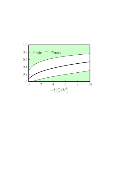
Figure 18: Region of $x$ (white region) which accounts for $90\%$ of $F_{2}^{p}(t)$ in our default fit for $E_{v}^{q}(x,t)$. The upper and lower shaded $x$-regions each account for $5\%$ of $F_{2}^{p}(t)$. The thick line shows the average $\langle x\rangle_{t}$ in the form factor integral.

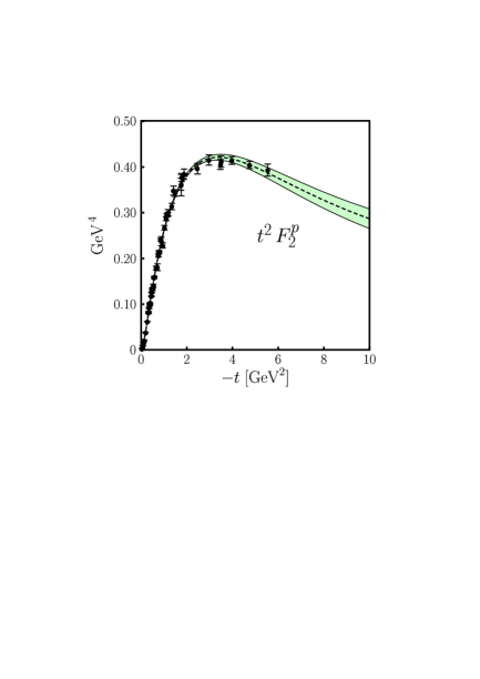
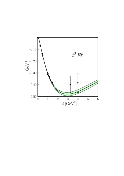
Figure 19: Results for the Pauli form factor of proton and neutron with our default fit defined in the text. The error bands represent the $1\,\sigma$ uncertainties of the fit as explained in App. B.

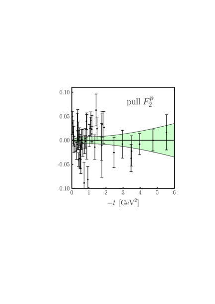
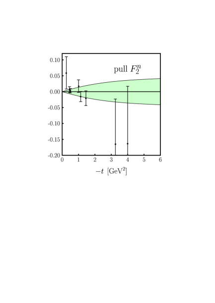
Figure 20: The pull $[F_{2}({\rm data})/F_{2}({\rm fit})-1]$ for our default fit to the Pauli form factors of the nucleon. The error bands represent the $1\,\sigma$ fit uncertainty relative to the best fit.

To quantify the sensitivity of our fit to the range of $x$ in the sum rules (46) we plot in Fig. 18 the quantities $x_{\rm min}(t)$, $x_{\rm max}(t)$ and $\langle x\rangle_{t}$ for the Pauli form factor of the proton, defined in analogy to (24) and (25) by replacing $H_{v}^{q}$ with $E_{v}^{q}$ and $F_{1}^{p}$ with $F_{2}^{p}$. We find that we are sensitive to values up to about $x\sim 0.7$ with the form factor data at hand. In Fig. 19 we show the result of our fit in comparison with the data, and in Fig. 20 the corresponding pull. With the exception of three (somewhat outlying) data points, our fit describes $F_{2}^{p}$ within 5% over the entire $t$ range. The description of $F_{2}^{n}$ is of similar quality, except for the two data points with the highest $-t$, where the central value of the fit is just compatible with the errors of the data.

5.4 Flavor structure

The fit we have just described exhibits a clear difference in the parameters of the $u$ and the $d$ quark distributions. To test the significance of this result, we have performed a fit with the same $\beta_{q}$, $C_{q}$ and $D_{q}$ for both flavors, leaving also $\alpha$ as a free parameter in order not to be biased by its particular value. The bounds (68) imply of course $C_{q}\leq 1.22\,{\rm GeV}^{-2}$ in this case. Such a fit does not give a satisfactory description of the neutron data, with a $\chi^{2}$ of 106 for the 8 data points according to Table 14. This fit undershoots all data for $|F_{2}^{n}|$ with $-t$ below $1.5\,{\rm GeV}^{2}$ by 5% to 10%, which is a large effects given the errors on the data in that region (see App. A). To see whether the positivity constraints are responsible for this failure, we have repeated the fit without restricting $C_{q}$. The fit then selects parameters $C_{q}$ and $\beta_{q}$ that badly violate the positivity constraints, but the resulting $F_{2}^{n}$ is barely changed for $-t<2\,{\rm GeV}^{2}$ and thus equally inadequate.

Having seen that the data and errors we use require different $\kappa_{u}^{-1}E_{v}^{u}$ and $\kappa_{d}^{-1}E_{v}^{d}$, we would like to explore for which of our parameters a flavor dependence is required most. From the fits with fixed $\beta_{u}$ and $\beta_{d}$ presented in Tables 1 and 12 we have already seen that $\kappa_{u}^{-1}e_{v}^{u}(x)=\kappa_{d}^{-1}e_{v}^{d}(x)$ for the forward limit is compatible with existing data. Concerning the profile functions, one may ask whether the data can be described when taking $D_{u}=D_{d}$, as was the case for the analogous fits of $H_{v}^{q}$. A fit with free $\beta_{u}$ and $\beta_{d}$ and this constraint selects $\beta_{d}$ much too small to comply with the positivity bound (62), so that instead we have performed a series of fits with fixed $\beta_{u}$ and $\beta_{d}$, leaving free parameters $D_{u}=D_{d}$ in addition to $C_{u}$ and $C_{d}$ subject to (68). The resulting values of $\chi^{2}/\mathrm{d.o.f.}$ are given in Table 2 and details of selected fits in Table 15. We find that a good description of both proton and neutron data is possible only if $\beta_{u}$ is significantly larger than $\beta_{d}$. In analogy to the discussion at the end of Sect. 5.3, this can again be understood from the necessity of the fit to accommodate $\kappa_{u}^{-1}F_{2}^{u}<\kappa_{d}^{-1}F_{2}^{d}$ at small $t$. In Table 15 we observe that with increasing $\beta_{u}$ the fit requires smaller and smaller profile functions $g_{u}(x)$, otherwise $F_{2}^{u}$ would decrease too fast to be compatible with the proton data at larger values of $t$. For the largest $\beta_{u}$ in the table this does not seem a physically very plausible scenario. In the case $\beta_{u}=11$ and $\beta_{d}=5$ the fitted values even lead to $g_{u}(x)<0$ for $0.5<x<0.8$, so that the corresponding entry in Table 2 has been omitted.

Table 2: Values of $\chi^{2}/\mathrm{d.o.f.}$ obtained in fits as specified in Table 1 but with the additional constraint $D_{u}=D_{d}$.

	$\beta_{u}$
	5	6	7	8	9	10	11
$\beta_{d}$	$\chi^{2}/\mathrm{d.o.f.}$
5	5.86	3.01	1.98	1.72	1.62	1.60
6	8.94	4.85	2.96	2.12	1.84	1.72	1.67

We have finally performed a series of fits where we imposed $C_{u}=C_{d}$ with the constraint $C_{q}\leq 1.22\,{\rm GeV}^{-2}$, summarized in Table 16. Provided that we allow a flavor dependence of either $\beta_{q}$ or $D_{q}$, a reasonably good description of the data can be achieved, although the $\chi^{2}$ for the neutron data is rather high.

We note that positivity restricts $E_{v}^{u}$ and $E_{v}^{d}$ in a rather asymmetric way. The bound (62) is stronger for $d$ quarks, given the stronger decrease of $d_{v}(x)$ with $x$. With the profile functions $f_{q}(x)$ from our default fit of $H_{v}^{q}$ one needs at least $\beta_{d}\geq 5$, whereas $\beta_{u}$ may be as small as $3.5$. For the parameters of the profile function, the constraint (63) is in turn more restrictive on $u$ quarks. We have seen that even with these constraints the flavor structure of the forward limit and of the profile function in $E_{v}^{q}$ cannot be uniquely determined by present data on the Pauli form factors. The neutron data can exclude a complete flavor independence of the distributions (up to their normalization) and somewhat disfavors a flavor independent profile function towards larger $x$. Flavor independence of $g_{q}$ at small to moderate $x$ cannot be excluded from the data, but it requires a rather extreme behavior of $E_{v}^{u}$. In view of these uncertainties, precise data on $F_{2}^{n}$ in a wider $t$ range would be of great help.

In Fig. 21 we plot the average sideways shift $s_{q}(x)$ of the distance between struck quark and spectators in a transversely polarized proton, obtained with different values of $\beta_{u}$ and $\beta_{d}$ for which satisfactory fits to the Pauli form factors can be obtained. Despite the considerable spread of possibilities, comparison with Fig. 5 shows that $|s_{q}(x)|$ is clearly below $d_{q}(x)$ for all $x$ where we can trust our results.

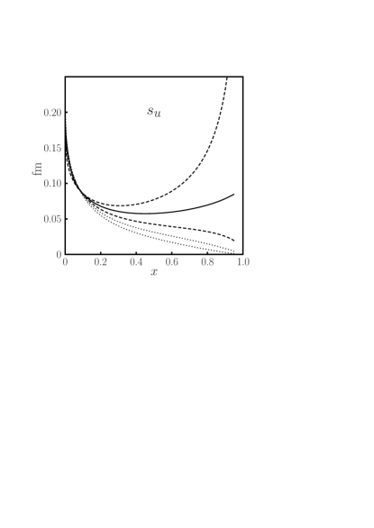
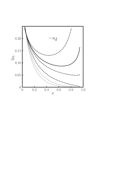
Figure 21: Average shift $s_{q}(x)$ of the distance between struck quark and spectators in a polarized proton, defined in (52). Solid curves correspond to the default fit (69), dashed curves to $\beta_{u}=3.5,4.5$ or $\beta_{d}=5,6,7$, and dotted curves to $\beta_{u}=5,5.5$ or $\beta_{d}=8,9$. In all cases $\alpha=0.55$.

6 Results for valence GPDs and their moments

In this section we present the results for the valence GPDs at zero skewness which follow from our default fits to the proton and neutron form factors.

6.1 GPDs as a function of $x$ and $t$

In Fig. 22 we have plotted $H_{v}^{u}(x,t)$ and $H_{v}^{d}(x,t)$ as functions of $x$ for some fixed values of momentum transfer $t$. We recall that the distributions in our default fits refer to the scale $\mu=2\,{\rm GeV}$. Notice the qualitative change when going from small to large values of $|t|$. For momentum transfer well below $1\,{\rm GeV}^{2}$ the GPDs resemble the forward parton distributions and in particular show a divergent behavior at small $x$. For increasing momentum transfer, the GPDs become narrower and develop a pronounced maximum, which shifts towards higher values of $x$ in accordance with the behavior of $\langle x\rangle_{t}$ in Fig. 2. The height of this maximum decreases with $|t|$, and this effect is more dramatic for $d$ quarks than for $u$ quarks. This can be traced back to our fit result for the profile functions, where $f_{d}(x,t)>f_{u}(x,t)$ at large $x$. The dashed lines in Fig. 22 indicate the values of $x$ where according to Fig. 2 the sensitivity of the form factor fits is not sufficient to constrain the GPDs, and therefore the result should be viewed as an extrapolation which follows from our particular ansatz for the functional form of the $x$ and $t$ dependence.

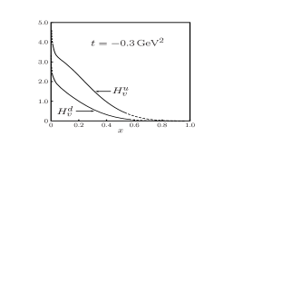
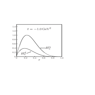
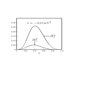
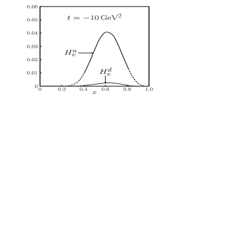
Figure 22: Result for the valence GPDs $H_{v}^{q}(x,t)$ at $\mu=2\,{\rm GeV}$ obtained in default fit to $F_{1}^{p}(t)$ and $F_{1}^{n}(t)$. Dashed lines indicate the regions where $x<x_{\rm min}(t)$ or $x>x_{\rm max}(t)$, see (24) and Fig. 2.

Figure 23: The same as Fig. 22 for the polarized valence GPDs $\widetilde{H}_{v}^{q}$.

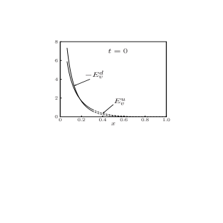
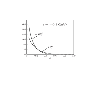
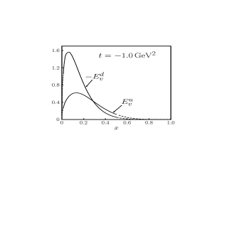
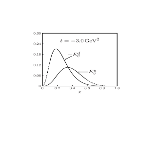
Figure 24: The same as Fig. 22 for the valence GPDs $E_{v}^{q}$. Dashed lines indicate the regions where $x<x_{\rm min}(t)$ or $x>x_{\rm max}(t)$ according to Fig. 18.

The same exercise is repeated for $\widetilde{H}_{v}^{u}(x,t)$ and $\widetilde{H}_{v}^{d}(x,t)$ in Fig. 23. Since we take the same profile functions for $H_{v}^{q}$ and $\widetilde{H}_{v}^{q}$, the qualitative behavior with increasing $|t|$ is similar for both cases. Remember that for $\widetilde{H}_{v}$ our imprecise knowledge of the polarized parton densities represents a major source of uncertainty.

In Fig. 24 we show the corresponding plots for the helicity-flip distributions $E_{v}^{u}(x,t)$ and $E_{v}^{d}(x,t)$ obtained in our default fit to the Pauli form factors $F_{2}^{p}$ and $F_{2}^{n}$. Again we observe a remarkably different behavior for $u$ and $d$ quarks. At $t=0$ the distributions $e_{v}^{u}(x)$ and $-e_{v}^{d}(x)$ are not too different, but for intermediate $|t|$ the distribution for $d$ quark develops a maximum which is more pronounced and located at significantly smaller $x$ than in the $u$ quark distribution. At larger values of $|t|$ we observe again a faster decrease of the $d$ quark distribution. This is because our default fits have equal values for the parameters $A_{q}$ and $C_{q}$, which respectively govern the large-$x$ behavior of the profile functions in $H_{v}^{q}$ and $E_{v}^{q}$.

6.2 Moments of GPDs

Important quantities obtained from GPDs are their moments in $x$. For zero skewness we define moments of valence GPDs as

$$h^{q}_{n,0}(t) = \int_{0}^{1}{\rm d}x\,x^{n-1}\,H_{v}^{q}(x,t)\ ,$$

$$\tilde{h}^{q}_{n,0}(t) = \int_{0}^{1}{\rm d}x\,x^{n-1}\,\widetilde{H}_{v}^{q}(x,t)\ ,$$

$$e^{q}_{n,0}(t) = \int_{0}^{1}{\rm d}x\,x^{n-1}\,E_{v}^{q}(x,t)\ .$$ (70)

In terms of the notation for moments used in [63, 19] we have

$$h^{q}_{n,0}(t)=A^{q}_{n,0}(t) e^{q}_{n,0}(t)=B^{q}_{n,0}(t)\hskip 30.00005pt\mbox{for odd $n$},$$ ,

$$\tilde{h}^{q}_{n,0}(t)=\tilde{A}^{q}_{n,0}(t) \hskip 101.00021pt\mbox{for even $n$}.$$ (71)

For even $n$ the moments $h^{q}_{n,0}$ and $e^{q}_{n,0}$ are not form factors of local operators, but can rather be seen as the valence contributions to the corresponding moments $A^{q}_{n,0}$ and $B^{q}_{n,0}$, which involve both valence and sea quarks. Likewise, $\tilde{h}^{q}_{n,0}$ is the valence contribution to $\tilde{A}^{q}_{n,0}$ when $n$ is odd. Note that for the lowest moments we just have $h^{q}_{1,0}=F_{1}^{q}$ and $e^{q}_{1,0}=F_{2}^{q}$.

In Fig. 25 we have plotted the first three moments of $H_{v}^{u}$ and $H_{v}^{d}$. The scaled $u$ quark moments $t^{2}h_{n,0}^{u}(t)$ show a similar behavior as the Dirac form factor of the proton, with a smooth increase up to values of about $-t=5\,{\rm GeV}^{2}$ and a rather flat plateau between $10\,{\rm GeV}^{2}\leq-t\leq 30\,{\rm GeV}^{2}$. On the other hand, the lowest $d$ quark moments $t^{2}h_{n,0}^{d}(t)$ have a pronounced maximum around $-t=3\,{\rm GeV}^{2}$ and die out much faster for higher values of $-t$. This can be understood in terms of the soft Feynman mechanism, or more precisely of the Drell-Yan relation, which relates a large-$x$ behavior like $(1-x)^{\beta}$ of a forward parton distribution with a large-$t$ behavior like $|t|^{-(1+\beta_{q})/2}$ of the associated form factor, see Sect. 3.5. Since $d_{v}(x)$ behaves approximately like $(1-x)^{5}$ at large $x$, we expect that $t^{2}h_{n,0}^{d}(t)\sim|t|^{-1}$ at intermediate values of $|t|$, which is roughly what we observe in Fig. 25.

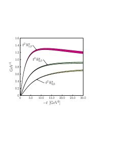
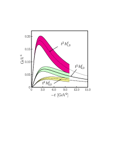
Figure 25: The first three moments of the valence GPDs $H_{v}^{u}$ (left) and $H_{v}^{d}$ (right), scaled with $t^{2}$. The error bands denote the parametric uncertainty resulting from the fit to the Dirac form factors $F_{1}^{p}$ and $F_{1}^{n}$.

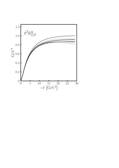
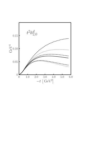
Figure 26: Systematic uncertainties for $n=2$ moments of valence GPDs $H_{v}^{q}$. The different line styles represent alternative fits to the Dirac form factors, as specified in the caption of Fig. 11.

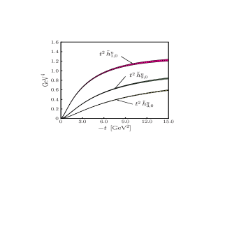
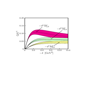
Figure 27: The first three moments of the valence GPDs $\widetilde{H}_{v}^{u}$ (left) and $\widetilde{H}_{v}^{d}$ (right), scaled with $t^{2}$. The error bands denote the parametric uncertainty of our default fit.

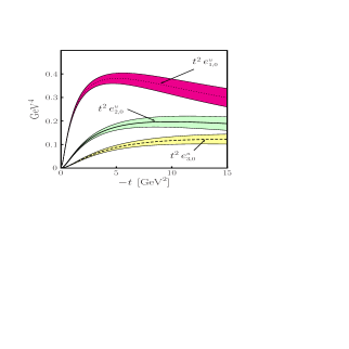
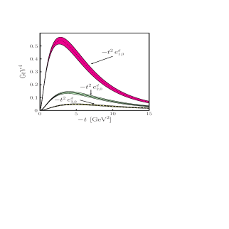
Figure 28: The first three moments of the valence GPDs $E_{v}^{u}$ (left) and $E_{v}^{d}$ (right), scaled with $t^{2}$. The error bands denote the parametric uncertainty resulting from our fit to the Pauli form factors $F_{2}^{p}$ and $F_{2}^{n}$.

The parametric errors on $h_{n,0}^{u}$ are rather small, reflecting the quality of the experimental data on the proton form factor. On the other hand the uncertainties on $h_{n,0}^{d}$ become large for $|t|$ above, say, $10~{}{\rm GeV}^{2}$, which is due to the lack of data on the neutron form factor in that region. In addition, we have to be aware of the systematic effects related to different choices or constraints for the profile functions. In Fig. 26 we study these effects by comparing the results for the moments $h_{2,0}^{q}$ from different fits to the Dirac form factor data, as we did for the distance function $d_{q}(x)$ in Fig. 11. We see that the systematic error for $u$ quark moments is reasonably small, whereas for $d$ quarks the uncertainty on individual moments above $|t|=3\,{\rm GeV}^{2}$ becomes very large. We should mention that in ratios of moments for the same quark flavor the systematic effects drop out to some extent.

For $\tilde{h}_{n,0}^{q}$ and $e_{n,0}^{q}$, which are shown in Figs. 27 and 28, similar comments concerning the $t$ dependence apply. We should point out that the moments $\tilde{h}_{n,0}$ are subject to additional uncertainties due to the polarized parton densities $\Delta q_{v}(x)$, which are not shown for simplicity. In the case of $e_{n,0}^{q}$ the rather large systematic uncertainties discussed in Section 5.2 should be kept in mind. We remark that for our default fit to the Pauli form factors, the powers governing the large-$x$ behavior of the forward distributions $e_{v}^{q}(x)$ are $\beta_{u}\simeq 4$ and $\beta_{d}\simeq 5.6$. Via the Drell-Yan relation this translates into a power behavior $e_{n,0}^{u}\sim|t|^{-2.5}$ and $e_{n,0}^{d}\sim|t|^{-3.3}$ in the region where the soft Feynman mechanism applies. As we can see from Fig. 28, this behavior sets in for values of $|t|$ above $5$ GeV², which is at the border of the region presently covered by experiment. Measurements of $F_{2}^{p}$ and $F_{2}^{n}$ up to momentum transfers of, say, $10$ GeV² could rather directly probe the region of the Feynman mechanism and thus provide valuable constraints on the exponents $\beta_{u}$ and $\beta_{d}$. The $t$ dependence of the presently available data probes the distributions in the transition region between small and large $x$.

The lowest moments of GPDs have been calculated in lattice QCD. In particular, the moments $A_{2,0}^{q}$ and $B_{2,0}^{q}$ for $u$ and $d$ quarks have been obtained in [8] for $-t$ up to $3\,{\rm GeV}^{2}$. The result has been parameterized in terms of a simple dipole fit with a common dipole mass $M=1.11\pm 0.20\,{\rm GeV}$ for all $n=2$ moments. One should keep in mind that the value of $M$ has been obtained by linear extrapolation to the chiral limit of results obtained with rather high pion (or equivalently quark) masses. Furthermore, we have evaluated the valence quark contributions to $A_{2,0}^{q}$ and $B_{2,0}^{q}$, whereas the lattice calculation includes sea quark effects to the extent that they are included in connected diagrams and in the quenched approximation of QCD. In Fig. 29 we compare our result for the normalized moments $h_{2,0}^{q}(t)/h_{2,0}^{q}(0)$ and $e_{2,0}^{q}(t)/e_{2,0}^{q}(0)$ with the dipole fit to the lattice results. Within their uncertainties the results are in remarkable agreement. As already pointed out, our analysis leads to quite different behavior of $u$ and $d$ quarks. In particular, $h_{2,0}^{d}$ falls of significantly faster than $h_{2,0}^{u}$. It will be interesting to see whether this effect is also observed in the improved lattice calculations currently under way.

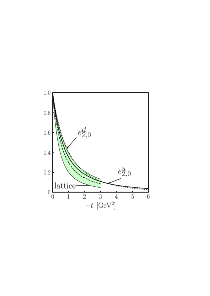
Figure 29: Comparison between lattice QCD results [8] and our default fit for the normalized moments $h_{2,0}^{q}(t)/h_{2,0}^{q}(0)$ and $e_{2,0}^{q}(t)/e_{2,0}^{q}(0)$. The dashed line with the band represents a fit to the lattice data with a common dipole mass $M=1.11\pm 0.20~{}{\rm GeV}$ for all $n=2$ moments.

6.3 Valence contribution to Ji’s sum rule

Our determination of the GPDs $E_{v}^{q}(x,t)$ from the fit to the Pauli form factors of proton and neutron has enabled us to estimate the forward distributions $e_{v}^{q}(x)$, which are not accessible in inclusive processes but play an essential role in understanding how the total spin of the nucleon is made up from quarks and gluons. The forward distributions $e_{v}^{q}(x)$ enter the angular momentum sum rule [1] in the form

$$2\langle L_{v}^{q}\rangle=\int_{0}^{1}{\rm d}x\Big{[}xe_{v}^{q}(x)+xq_{v}(x)-\Delta q_{v}(x)\Big{]}\,,$$ (72)

where we have only given the contribution from valence quarks. The second moments of unpolarized parton densities $q_{v}(x)$ are well-determined from DIS and other inclusive processes. The first moments of polarized parton densities can be obtained from the axial-vector couplings of nucleons and hyperons under the assumption that the couplings satisfy flavor SU(3) symmetry and that the polarized quark sea is also SU(3) symmetric. For a recent analysis we refer to [64], whose results were also taken as an input for the polarized parton distributions of [21] used in this work. The contribution to (72) from the second moments of $e_{v}^{q}(x)$ can be computed from our default fit. For this particular quantity the systematic uncertainties are dominated by our insufficient knowledge on the power $\beta_{q}$ used in the ansatz (65). In comparison to this parameter, the power $\alpha$ in (65) is rather well determined.

In Fig. 30 we study the variation of the second moments $e_{2,0}^{q}$ at $t=0$ within the wide range of $\beta_{q}$ values for which we found consistent fits to the Pauli form factors. We observe that the contributions of $u$ and $d$ quarks are almost equal in magnitude (varying between $0.10$ and $0.15$) and opposite in sign. The corresponding relative uncertainties on the valence contributions to the orbital angular momentum are rather small. This is shown in Fig. 31, where we have used the unpolarized CTEQ6M distributions at $\mu=2\,{\rm GeV}$ and the results of [64] to evaluate the last two terms in (72). In the sum $\langle L_{v}\rangle=\langle L_{v}^{u}\rangle+\langle L_{v}^{d}\rangle$ the contributions from $u$ and $d$ quarks cancel to a large extent, so that the relative error on this quantity is bigger again. With the central values of $\beta_{u}$ and $\beta_{d}$ from our default fit we obtain $2\langle L_{v}\rangle\approx-0.17$ at $\mu=2\,{\rm GeV}$.

As we already mentioned, sea quarks do not enter the Pauli form factor and are thus not accessible in our fit for the GPDs. For completeness we note that the sea quark contributions to $2\langle L^{u}\rangle$ and $2\langle L^{d}\rangle$ at $\mu=2\,{\rm GeV}$ are $2\int{\rm d}x\,(x\bar{u}-\Delta\bar{u})\approx-0.09$ and $2\int{\rm d}x\,(x\bar{d}-\Delta\bar{d})\approx-0.08$ if we take the distributions from CTEQ6M [20] and the NLO distributions in scenario 1 of [21]. Since we have no information on the sea quark contributions corresponding to the first term in (72), we refrain from comparing our results with evaluations of $\langle L^{q}\rangle$ in lattice QCD [8, 9, 65].

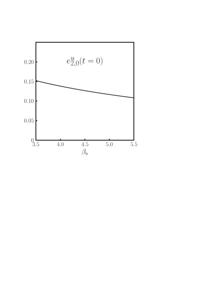
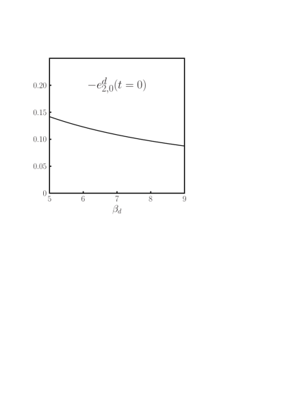
Figure 30: Variation with $\beta_{q}$ of the second moment of $e_{v}^{q}(x)$ at $\mu=2\,{\rm GeV}$.

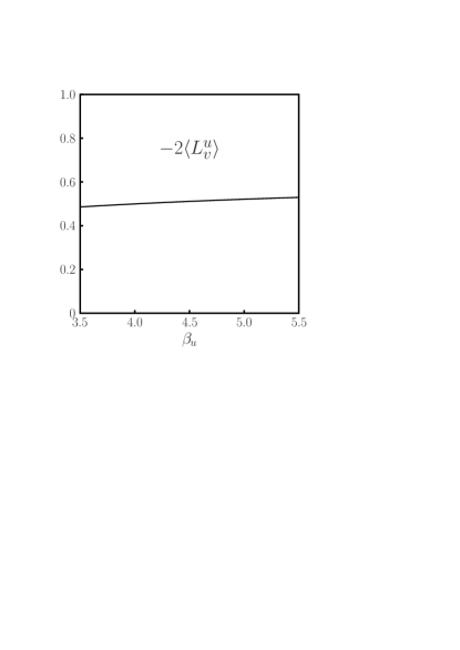
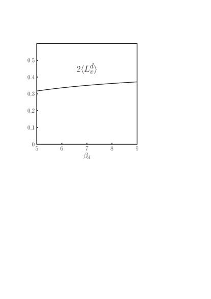
Figure 31: As in Fig. 30 but for the valence contribution to $2\langle L^{q}\rangle$ at $\mu=2\,{\rm GeV}$.

6.4 Proton tomography

In Figs. 32 and 33 we illustrate our default results for GPDs as tomography plots in impact parameter space for fixed longitudinal momentum fraction $x$. We show the unpolarized density $q_{v}(x,\mbox{\boldmath{$b$}})$ as well as its analog $q_{v}^{X}(x,\mbox{\boldmath{$b$}})$ for a proton polarized in the $x$ direction, see (3) and (48). Notice that in general $q_{v}^{X}(x,\mbox{\boldmath{$b$}})$ has no rotational symmetry in the impact parameter plane, as is readily seen from (48). One can nicely see that the displacement of the center of the distribution along the $b^{y}$ axis is different for $u$ and $d$ quarks. According to our discussion in Section 5 the average displacement is described by the quantity $s_{q}(x)$ defined in (52). Indeed we read off from Fig. 21 that for small values of $x$ the shift $|s_{d}(x)|$ in our default fit is significantly larger than $s_{u}(x)$. This explains the pronounced difference between the polarized and unpolarized densities $d_{v}^{X}(x,\mbox{\boldmath{$b$}})$ and $d_{v}(x,\mbox{\boldmath{$b$}})$ at small $x$ compared to the corresponding $u$ quark densities. The different signs of $s_{u}(x)$ and $s_{d}(x)$, corresponding to the different signs of the anomalous magnetic moments $\kappa_{u}$ and $\kappa_{d}$, imply that for $d$ quarks the center of the polarized density is shifted toward negative $b_{y}$, whereas for $u$ quarks it is found at positive $b_{y}$.

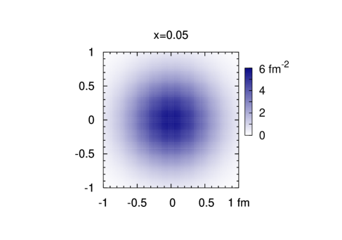
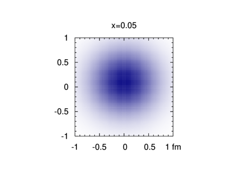
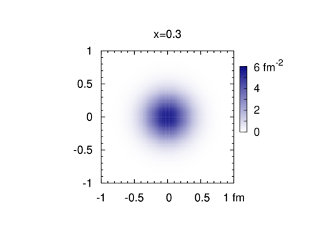
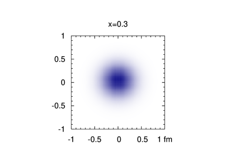
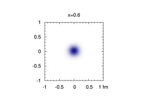
Figure 32: Tomography plots of $u_{v}(x,\mbox{\boldmath{$b$}})$ (left) and $u_{v}^{X}(x,\mbox{\boldmath{$b$}})$ (right) in the transverse $b^{x}$–$b^{y}$ plane. Note that the scale of intensity for longitudinal momentum fraction $x=0.6$ differs from the one for $x=0.3$ and $x=0.05$.

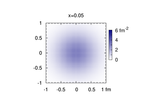
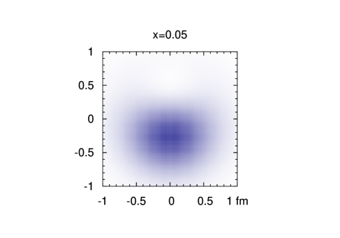
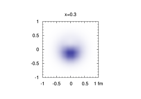
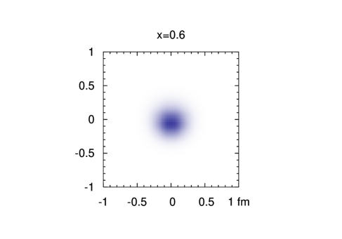
Figure 33: Tomography plots of $d_{v}(x,\mbox{\boldmath{$b$}})$ (left) and $d_{v}^{X}(x,\mbox{\boldmath{$b$}})$ (right) in the transverse $b^{x}$–$b^{y}$ plane. Note that the scale of intensity is different for all three longitudinal momentum fractions $x$.

7 Handbag approach to wide-angle Compton scattering

Our analysis in Sect. 3.5 has shown that at momentum transfer $-t$ around $10\,{\rm GeV}^{2}$ the proton Dirac form factor can be described in terms of the soft Feynman mechanism. Dominance of this mechanism is the basis of the so-called handbag approach to wide-angle Compton scattering [4, 5] and related processes [66, 67]. In this approach the relevant process amplitudes factorize into a hard scattering on a single quark in the target and moments of GPDs at skewness $\xi=0$. The handbag approach is restricted to kinematical situations where all Mandelstam variables $s$, $t$, $u$ are sufficiently large compared to a hadronic scale $\Lambda^{2}$, but not yet in the asymptotic regime where the standard hard-scattering approach [47] is applicable. Before turning to a quantitative analysis of the Compton form factors on the basis of our results from Section 3, we wish to clarify some important theoretical aspects, concerning in particular the inclusion and interpretation of radiative QCD corrections in the handbag formalism. A formal proof for handbag factorization would require a systematic treatment of these corrections, an issue which has not been addressed in too much detail yet. As a first step, one-loop radiative corrections to the partonic scattering amplitude in Compton scattering have been evaluated in [68, 69].

7.1 Compton scattering and Compton form factors

Let us recall some important features of the handbag approximation to Compton scattering, $\gamma p\to\gamma p$, at large angles. (The discussion in this and the following subsection can be generalized to the case where the incoming photon is off-shell.) The approximation assumes that the soft configurations discussed in Sect. 3.5 are dominant in the scattering process. The process amplitude can then be written in terms of hard-scattering amplitudes for Compton scattering on a free quark, $\gamma q\to\gamma q$, multiplied with Compton form factors describing the emission and reabsorption of the struck quark by the proton target. The form factors are given in terms of GPDs as

$$R_{V}(t,\mu^{2}) = \sum_{q}e_{q}^{2}\,\int_{-1}^{1}\frac{{\rm d}x}{x}H^{q}(x,t,\mu^{2})\ ,\qquad\qquad R_{T}(t,\mu^{2})\>=\>\sum_{q}e_{q}^{2}\,\int_{-1}^{1}\frac{{\rm d}x}{x}E^{q}(x,t,\mu^{2})\ ,$$

$$R_{A}(t,\mu^{2}) = \sum_{q}e_{q}^{2}\,\int_{-1}^{1}\frac{{\rm d}x}{x}\,\mbox{sgn}(x)\,\widetilde{H}^{q}(x,t,\mu^{2})\ ,$$ (73)

with the momentum fraction $x$ defined in a frame where the plus-momentum of the proton is equal before and after the scattering, see Sect. 3.5 and [5]. The derivation of the factorization formula requires approximations appropriate for the soft kinematics specified in (3.5), where terms suppressed by $\Lambda/\sqrt{|t|}$ are neglected. In particular, the amplitudes for the partonic subprocess $\gamma q\to\gamma q$ are evaluated with the four-momentum $k$ of the struck quark approximated by the full momentum $p$ of the proton (see Fig. 12a for the kinematics). The Mandelstam variables $\hat{s}$, $\hat{t}$, $\hat{u}$ of the subprocess $\gamma q\to\gamma q$ are then equal to the Mandelstam variables $s$, $t$, $u$ of the overall process $\gamma p\to\gamma p$. The longitudinal momentum fraction $x$ of the struck quark is thus set to $1$ in the hard-scattering amplitude, leaving the integration over $x$ to be performed at the level of the proton matrix elements as given in (7.1). The results of our phenomenological fit for $H_{v}^{q}(x,t)$ show that at $-t$ of several $\,{\rm GeV}^{2}$ the proton matrix elements are not dominated by very large values of $x$. In Fig. 22 we see for instance that at $-t=10\,{\rm GeV}^{2}$ the maximum of $H_{v}^{u}(x,t)$ is around $x\approx 0.62$, with half the maximum attained at $x\approx 0.47$ and $x\approx 0.77$. This is well within the parametric estimate $(1-x)\sim\Lambda/\sqrt{|t|}$ if we take for $\Lambda$ a value around $1\,{\rm GeV}$, but one may worry that the resulting approximation of the hard-scattering amplitude is very bad. This need not necessarily be the case. To see this, let us consider more sophisticated relations between $\hat{s}$, $\hat{t}$, $\hat{u}$ and $s$, $t$, $u$. The ansatz $\hat{s}=xs$ and $\hat{u}=xu$ for instance can be argued to give a better first approximation than the naive relation with $x=1$. Since the leading-order scattering kernels for $\gamma q\to\gamma q$ depend only on $\hat{u}/\hat{s}$, the value of $x$ cancels in this approximation. A consistent treatment of the kinematics in the handbag graphs beyond the $x=1$ approximation must however be complemented by the inclusion of graphs that are not described by the proton matrix elements corresponding to the twist-two GPDs in (7.1). Such graphs involve for instance operators with two quark fields and an additional gluon, or four-quark operators associated with the so-called cat’s ears diagrams. The inclusion of higher-twist operators is already required to preserve electromagnetic gauge invariance of the Compton amplitude, as has been seen in the treatment of deeply virtual Compton scattering [71, 72]. A corresponding analysis for wide-angle scattering would be very important but has remained elusive so far.

A related theoretical uncertainty concerns the factor $1/x$ in the integrals (7.1). In the derivation of [5] it is somewhat ambiguous whether to associate this factor with the soft matrix elements or with the hard-scattering amplitude, where it would be approximated by 1. The difference between $1/x$ and $1$ is among the effects which are presently beyond theory control. Numerically it is quite large in the $t$ range of Compton scattering experiments, given that the expansion parameter $\Lambda/\sqrt{|t|}$ relevant for the soft Feynman mechanism only scales with the square root of the large momentum transfer. The expressions (7.1) should only be used for values of $t$ that are large enough for the underlying approximations—at small $t$ the corresponding integrals even diverge. As we observed at the end of Sect. 3.6, the valence GPDs from our ansatz with an exponential $t$ dependence vanish like a power of $x$ for $x\to 0$ provided that $|t|\raisebox{-4.0pt}{$\,\stackrel{{\scriptstyle\textstyle>}}{{\sim}}\,$}0.7\,{\rm GeV}^{2}$, so that their $1/x$ integrals then converge. However, sea quarks also contribute to the Compton form factors, which describe exchange of positive $C$ parity in the $t$-channel. Since in the distributions at $t=0$ the small-$x$ rise is faster for sea quarks than for valence quarks, one expects that larger $|t|$ is necessary to make (7.1) well defined. We shall return to the issue of sea quarks in Sect. 7.3.

The $1/x$ factors in (7.1), as well as the $\mbox{sgn}(x)$ in the case of $R_{A}$, give rise to a $\mu$ dependence of the Compton form factors. Arising from DGLAP evolution of the GPDs under the integral, this scale dependence is an effect of order $\alpha_{s}$. We shall see in the next subsection that at present NLO corrections to wide-angle Compton scattering are only understood in the approximation where $x$ is set to $1$ in the hard-scattering amplitude and where the form factors (7.1) are replaced with their scale independent counterparts

$$R_{V}^{(0)}(t) = \sum_{q}e_{q}^{2}\,\int_{-1}^{1}{\rm d}x\,H^{q}(x,t,\mu^{2})\ ,\qquad\qquad R_{T}^{(0)}(t)\>=\>\sum_{q}e_{q}^{2}\,\int_{-1}^{1}{\rm d}x\,E^{q}(x,t,\mu^{2})\ ,$$

$$R_{A}^{(0)}(t) = \sum_{q}e_{q}^{2}\,\int_{-1}^{1}{\rm d}x\,\widetilde{H}^{q}(x,t,\mu^{2})\,,$$ (74)

which apart from charge factors are just the usual Dirac, Pauli, and axial form factors. In addition to neglecting the difference between $1/x$ and $1$, we have counted antiquarks with the “wrong” sign in the integral over $\widetilde{H}^{q}$, which should again be a valid approximation when large enough momentum fractions dominate in the integral.

7.2 NLO corrections to wide-angle Compton scattering

Next-to-leading order corrections to the partonic subprocess in Compton scattering have been calculated in [68]. This means to consider virtual corrections to $\gamma q\to\gamma q$ where the virtualities of the loop momenta are hard, i.e., where they scale with the large momentum transfer $t$. The unrenormalized result for the hard-scattering amplitudes has the schematic form

$${\cal H}^{\rm LO}(s,t)\left(1+\frac{\alpha_{s}C_{F}}{4\pi}\,C_{\rm IR}(t,\mu^{2})\right)+\frac{\alpha_{s}C_{F}}{4\pi}\,{\cal H}^{\rm NLO}(s,t)\ ,$$ (75)

where the NLO contribution has been decomposed into a divergent part $C_{\rm IR}(\mu,t)$ multiplied with the LO amplitude and a finite piece ${\cal H}^{\rm NLO}(s,t)$. Using dimensional regularization with $D=4+\epsilon$, one has

$$C_{\rm IR}(t,\mu^{2})=-\frac{8}{\epsilon^{2}}+\frac{4}{\epsilon}\ln\frac{\mu^{2}}{|t|}+\frac{6}{\epsilon}-\ln^{2}\frac{\mu^{2}}{|t|}-3\ln\frac{\mu^{2}}{|t|}+\mbox{constant terms}\,,$$ (76)

which contains a collinear and a soft infrared divergence, and the well-known Sudakov double logarithms. It has been pointed out in [68] that the soft and collinear divergences and the associated double logarithms are universal: not only do they appear in the corrections to $\gamma q\to\gamma q$ but also in the corrections to $\gamma^{*}q\to q$, which are relevant for the elastic proton form factors. In a “physical” factorization scheme one considers the radiative corrections to the quark-photon vertex as part of the form factor itself. To renormalize the Compton form factors and the corresponding hard-scattering amplitudes one then subtracts the full expression $C_{\rm IR}$, where the constant terms are fixed by the condition that in this scheme the elastic proton form factor is unchanged. Writing the overall Compton amplitudes as $M_{i}$, where $i$ corresponds to the subscripts $V$, $A$, $T$ of the Compton form factors, we then have

$$M_{i}(s,t) = \left({\cal H}_{i}^{\rm LO}(s,t)+\frac{\alpha_{s}C_{F}}{4\pi}\,{\cal H}_{i}^{\rm NLO}(s,t)\right)R_{i}(t,\mu^{2})+\ldots$$ (77)

$$= \left({\cal H}_{i}^{\rm LO}(s,t)+\frac{\alpha_{s}C_{F}}{4\pi}\,{\cal H}_{i}^{\rm NLO}(s,t)\right)R_{i}^{(0)}(t)+{\cal H}_{i}^{\rm LO}(s,t)\left[R_{i}^{\phantom{()\!\!}}(t,\mu^{2})-R_{i}^{(0)}(t)\right]+\ldots.\hskip 25.00003pt$$

Note that the NLO calculations for $\gamma q\to\gamma q$ and $\gamma^{*}q\to q$ with on-shell quarks enabled us to find a renormalization scheme at the level of the electromagnetic and weak nucleon form factors and of their flavor combinations (7.1) relevant for Compton scattering. They do not permit an analogous renormalization of the Compton form factors (7.1) or of the GPDs themselves. This is manifest in the first line of (77), where we have an uncanceled $\mu$ dependence. In the second line of (77) we have therefore indicated that, for internal consistency of the presently available results, the NLO calculation should be restricted to the part of the Compton form factors which involves the same local operators as $F_{1}$, $F_{2}$ and $F_{A}$. The parametric uncertainties of the second line in (77) are of order $\alpha_{s}^{2}$ or of order $\alpha_{s}\,\Lambda/\sqrt{|t|}$. Up to this accuracy the result is $\mu$ independent as it must be. Controlling effects of order $\alpha_{s}\,\Lambda/\sqrt{|t|}$ would require a more complete analysis of power-suppressed terms already at Born level.

Following an alternative point of view, one could use a minimal subtraction scheme in (75) to render the resummation of Sudakov logarithms explicit in hard coefficient functions. The Compton amplitudes would then be written as

$$M_{i}(s,t)=C_{i}(s,t,\mu^{2})\,R_{i}^{\rm eff}(t,\mu^{2})+\ldots,$$ (78)

where $C_{i}(s,t,\mu^{2})$ obeys the renormalization group equation

$$\mu^{2}\frac{{\rm d}}{{\rm d}\mu^{2}}\,C_{i}(s,t,\mu^{2})=\gamma(t,\mu^{2})\,C_{i}(s,t,\mu^{2})$$ (79)

whose anomalous dimension follows from (76),

$$\gamma(t,\mu^{2})=-\frac{\alpha_{s}C_{F}}{2\pi}\left(\ln\frac{\mu^{2}}{|t|}+\gamma_{0}\right)+{\cal O}(\alpha_{s}^{2})\ .$$ (80)

The value of the constant $\gamma_{0}$ depends on the renormalization scheme. Renormalization group evolution from $\mu^{2}\sim|t|$ down to $\mu_{0}^{2}\sim\Lambda\sqrt{|t|}$ corresponds to the summation of Sudakov logarithms between those two scales, which are then explicitly contained in $C_{i}(s,t,\mu_{0}^{2})$. In this sense, the new Compton form factors $R_{i}^{\rm eff}(t,\mu_{0}^{2})$ only contain dynamics below the factorization scale $\mu_{0}^{2}$, which is the virtuality of the struck quark in soft kinematics. They can be considered as being defined in soft-collinear effective theory [73, 74], which is an effective field theory where the hard degrees of freedom are integrated out, leaving degrees of freedom with virtualities smaller than $|t|$. The scale dependence of $R_{i}^{\rm eff}(t,\mu^{2})$ compensates that of $C_{i}(s,t,\mu^{2})$.

Similarly, in the effective theory the Dirac form factor can be written as

$$F_{1}(t)=C_{1}(t,\mu^{2})\,F_{1}^{\rm eff}(t,\mu^{2})+\ldots$$ (81)

with a hard coefficient function that obeys the same evolution equation as in the case of Compton form factors,

$$\mu^{2}\frac{{\rm d}}{{\rm d}\mu^{2}}\,C_{1}(t,\mu^{2})=\gamma(t,\mu^{2})\,C_{1}(t,\mu^{2}).$$ (82)

In other words, the function $C_{1}(t,\mu^{2})$ resums the same (leading) Sudakov logarithms as $C_{i}(t,\mu^{2})$. The physical scheme where the coefficient function in (81) is equal to 1 is related to a general scheme by a finite renormalization. Applying the same renormalization to the Compton form factors one would write

$$R_{i}^{(0)}(t)=C_{1}(t,\mu^{2})R_{i}^{\rm eff}(t,\mu^{2})+\ldots,$$ (83)

which together with (78) gives

$$M_{i}(s,t)=\frac{C_{i}(s,t,\mu^{2})}{C_{1}(t,\mu^{2})}\,R_{i}^{(0)}(t)+\ldots.$$ (84)

Sudakov effects cancel in the ratio of hard-coefficient functions, which can therefore be calculated in fixed-order perturbation theory as

$$\frac{C_{i}(s,t,\mu^{2})}{C_{1}(t,\mu^{2})}={\cal H}_{i}^{\rm LO}(s,t)+\frac{\alpha_{s}C_{F}}{4\pi}\,{\cal H}_{i}^{\rm NLO}(s,t)+\ldots,$$ (85)

where we recover (77) to leading accuracy in the expansion parameter $\Lambda/\sqrt{|t|}$ of the effective theory.

Returning to the level of GPDs, we have so far dealt with distributions $H_{v}^{q}(x,t,\mu^{2})$ defined by standard collinear renormalization in QCD. Note that even for $\mu^{2}\ll|t|$ such distributions can be defined, since they can be obtained from distributions with $\mu^{2}\raisebox{-4.0pt}{$\,\stackrel{{\scriptstyle\textstyle>}}{{\sim}}\,$}|t|$ by DGLAP evolution, which may be understood as a finite renormalization. The result does however not correspond to matrix elements with internal virtualities of at most $\Lambda\sqrt{|t|}$, which would be appropriate for the soft Feynman mechanism. One may speculate that such a “soft GPD” would be obtained in the effective theory as

$$H_{v}^{q\,\rm eff}(x,t,\mu^{2})=\frac{1}{C_{1}(t,\mu^{2})}\,H_{v}^{q}(x,t,\mu^{2})$$ (86)

for $|t|\gg\Lambda^{2}$, with associated sum rules

$$F_{1}^{\rm eff}(t,\mu^{2})=\sum_{q}e_{q}\int_{0}^{1}{\rm d}x\,H_{v}^{q\,\rm eff}(x,t,\mu^{2}),\qquad R_{V}^{\rm eff}(t,\mu^{2})=\sum_{q}e_{q}^{2}\int_{0}^{1}{\rm d}x\,H_{v}^{q\,\rm eff}(x,t,\mu^{2}).$$ (87)

Notice that $H_{v}^{q\,\rm eff}$ obeys a different evolution equation than $H_{v}^{q}$, since its renormalization includes the Sudakov logarithms from the endpoint region $x\to 1$. It is however not clear whether the $x$-independent renormalization factor in (86) corresponds indeed to the structure emerging in the effective theory.

In the absence of a proper definition for “soft GPDs”, we understand the distributions extracted in this work as “standard GPDs” obeying DGLAP evolution. This is also convenient in connection with our phenomenological ansatz (11), which interpolates between the standard $\overline{\mbox{MS}}$ parton densities at $t=0$ and distributions at large $t$. We point out that even for the highest values of $-t\sim 30\,{\rm GeV}^{2}$ we consider in our applications, Sudakov double logarithms are not very large, with $\ln^{2}(\mu^{2}/|t|)\leq 4$ for $\mu=2\,{\rm GeV}$, so that one may expect the difference between “soft” and “standard” GPDs to be reasonably small.

In our calculations for wide-angle Compton scattering we will use the form factors (7.1), regarding their $1/x$ factors as a phenomenological estimate of effects beyond a strict $\Lambda/\sqrt{|t|}$ expansion. To keep the analysis simple we have refrained from using the expression (77) and instead take the full form factors (7.1) multiplied with the hard-scattering amplitudes at NLO. Since the $\mu^{2}$ dependence inherent in the $1/x$ moments is an effect beyond present theoretical control, we will require that the variation of the form factors obtained with GPDs fitted for $\mu=1$, $2$ and $4\,{\rm GeV}$ remains reasonably small. This will provide a criterion of how large $t$ is required to obtain stable results within our present approach.

7.3 Results for form factors and observables

After our discussion of theoretical uncertainties let us now see how they quantitatively look like with the GPDs we have obtained from our fits to elastic form factors. We restrict this discussion to $R_{V}$, which dominates the unpolarized Compton cross section. In Fig. 34 we compare the full form factor $R_{V}$ and its analog $R_{V}^{(0)}$ without a factor of $1/x$ under the integral, both evaluated with the result of our default fit for $H_{v}^{q}(x,t)$. As is to be expected from the shape of $H_{v}^{q}$ in Fig. 22, the difference is considerable in the $t$ range relevant for existing or planned measurements. The error bands on the curves for $R_{V}$ and $R_{V}^{(0)}$ indicate the variation of $H_{v}^{q}$ with $\mu$, with the limits of the bands corresponding to the fits with $\mu=1$ and $4\,{\rm GeV}$ listed in Table 10. The scale variation for $R_{V}$ becomes rather large for $-t$ below about $3\,{\rm GeV}^{2}$, which gives a first indication of when effects of order $\alpha_{s}\,\Lambda/\sqrt{|t|}$ can no longer be neglected. The tiny scale dependence of $R_{V}^{(0)}$ confirms that our fits to $F_{1}^{p}$ and $F_{1}^{n}$ with input parton densities at different $\mu$ indeed give a scale invariant result to a very good approximation.

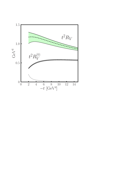
Figure 34: Study of systematic uncertainties regarding the Compton form factor $R_{V}$. Shown are $t^{2}R_{V}$ and $t^{2}R_{V}^{(0)}$ from (7.1) and (7.1) evaluated from our default fit for $H_{v}^{q}$ at $\mu=2\,{\rm GeV}$. The limits of the error bands correspond to the fits for $H_{v}^{q}$ at $\mu=1$ and $4\,{\rm GeV}$ in Table 10. The dotted line shows the sea quark contribution to $t^{2}R_{V}$ as specified before and in (88).

As we already mentioned, sea quark contributions do not cancel in the Compton form factors defined in (7.1). Contrary to the isovector axial form factor $F_{A}(t)$, the quark flavor combination in Compton scattering is also sensitive to the flavor singlet distribution, which is more difficult to model due to its mixing with gluons as explained at the end of Sect. 3.1. For a naive estimate we have taken the same impact parameter profile for sea quarks and valence quarks. We thus define ${H}^{\bar{q}}(x,t)=-H^{q}(-x,t)$ and set ${H}^{\bar{q}}(x,t)=\bar{q}(x)\exp[tf_{q}(x)]$ with the CTEQ6M [20] antiquark densities $\bar{q}(x)$ at $\mu=2\,{\rm GeV}$ and with $f_{q}(x)$ determined in our default fit for $H_{v}^{q}$. The resulting sea quark contribution

$$R_{V}^{\rm sea}(t,\mu^{2})=2\sum_{q}e_{q}^{2}\,\int_{0}^{1}\frac{{\rm d}x}{x}H^{\bar{q}}(x,t,\mu^{2})$$ (88)

to $R_{V}$ is shown as the dotted curve in Fig. 34, where we have restricted the sum over quark flavors $u$ and $d$. When the sea quark contribution becomes important, we are clearly outside the region where the physical picture and the approximations of the soft Feynman mechanism are applicable. We see that with our estimate one need not worry about sea quarks for $-t\geq 4\,{\rm GeV}^{2}$. Below $-t=2\,{\rm GeV}^{2}$ their contribution quickly grows out of control, and we will therefore not show Compton form factors below this value.

We have seen in Fig. 13 that our default fit for $H_{v}^{q}$ exhibits the scaling properties characteristic of the soft Feynman mechanism in $F_{1}^{p}(t)$ for $-t$ above $10\,{\rm GeV}^{2}$. Below this value one enters a transition region, where the scaling becomes more and more approximate. Figure 34 indicates that current theoretical control over the Feynman mechanism in wide-angle Compton scattering does not extend below $-t=2\,{\rm GeV}^{2}$.

In Fig. 35 we show the Compton form factors obtained from our default fits for $H_{v}^{q}$, $E_{v}^{q}$ and from the ansatz (44) for $\widetilde{H}_{v}^{q}$ with $\tilde{f}_{q}=f_{q}$. We plot both individual flavor contributions and the flavor combinations $R_{i}=\frac{4}{9}R^{u}_{i}+\frac{1}{9}R^{d}_{i}$ for Compton scattering on the proton. In the case of $R_{V}^{q}$ and $R_{A}^{q}$ we see the clear dominance of $u$ quarks over $d$ quarks even without the charge factors, as we already did for the corresponding moments in Sect. 6.2. The full form factors $R_{V}$ and $R_{A}$ turn out to be somewhat smaller than those modeled in [5].

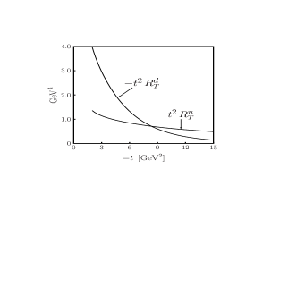
Figure 35: Scaled Compton form factors for individual quark flavors and summed with the appropriate squared charge factors (bottom right). The error bands shown for $R_{V}$ and for $R_{T}$ correspond to the $1\,\sigma$ uncertainties of our default fits for $H_{v}^{q}$ and $E_{v}^{q}$. The band for $R_{A}$ corresponds to the $1\,\sigma$ uncertainties on our profile function added in quadrature to the errors on the polarized parton densities in [21], which are by far dominant for this quantity.

For $R_{T}^{q}$ the relative weight of flavors is different than for $R_{V}^{q}$ and $R_{A}^{q}$. Even more than for the moments $e_{1,0}^{q}$ in Fig. 28, $d$ quarks dominate for smaller and $u$ quarks for larger values of $t$. Given the opposite signs of $R_{T}^{u}$ and $R_{T}^{d}$ and the squared charge factors, the resulting $R_{T}$ is significantly smaller than $R_{V}$ and $R_{A}$ at lower values of $t$. The ratio $R_{T}/R_{V}$ behaves quite differently from the analogous ratio $F_{2}^{p}/F_{1}^{p}$ of electromagnetic form factors. With

$$\kappa_{\rm C}(t)=\frac{\sqrt{-t}}{2m}\,\frac{R_{T}(t)}{R_{V}(t)}\,,\qquad\qquad\kappa_{\rm em}(t)=\frac{\sqrt{-t}}{2m}\,\frac{F_{2}^{p}(t)}{F_{1}^{p}(t)}\,,$$ (89)

the measurement of [76] gives an approximately constant $\kappa_{\rm em}\approx 0.37$ for $2\,{\rm GeV}^{2}\leq-t\leq 5.5\,{\rm GeV}^{2}$, whereas we find that with our default fits $\kappa_{\rm C}$ rises from 0.1 to 0.25 in the same interval and continues to grow to 0.4 at $-t=10\,{\rm GeV}^{2}$. Our result for $R_{T}$ is however subject to rather large uncertainties, given the considerable freedom we encountered in extracting $E_{v}^{q}$ from the Pauli form factors alone. The fits shown in Table 12, which all give a good description of $F_{2}^{p}$ and $F_{2}^{n}$, produce form factors $R_{T}$ which at $-t=5\,{\rm GeV}^{2}$ are up to a factor of 1.5 larger than $R_{T}$ shown in Fig. 35, with even larger discrepancies at lower $t$. Within this set of fits, the curve in the figure acts more like a lower bound.

With the form factors in Fig. 35 we obtain the unpolarized cross section $d\sigma/dt$ shown in Fig. 36 for a squared c.m. energy of $s=11\,{\rm GeV}^{2}$. We have included the NLO corrections in the physical scheme described in Sect. 7.2, subtracting a constant term $\frac{\alpha_{s}C_{F}}{4\pi}\left(\frac{\pi^{2}}{3}-8\right)$ from the quark scattering kernels of [68] as mentioned in footnote 4. For the form factor $R_{V}^{g}$ describing gluon exchange at NLO we have taken the model result of [68] divided by a factor of 1.3, which is the typical discrepancy at $-t\sim 5\,{\rm GeV}^{2}$ between $R_{V}$ obtained in the present study and in [68]. The resulting gluonic contribution to $d\sigma/dt$ is only a few percent.

The inner band for the curve of $d\sigma/dt$ reflects the parametric errors on the form factors shown in Fig. 35. The corresponding uncertainty is very small. This is because $R_{V}$ is strongly dominated by $H_{v}^{u}$, which is the distribution best constrained by the abundant data for $F_{1}^{p}$, whereas the individual contributions of both $R_{A}$ and $R_{T}$ to $d\sigma/dt$ are between 1% and 10% for the kinematics shown in Fig. 36. The central curve in the figure corresponds to scenario 2 in [77], where the Mandelstam variables of $\gamma q\to\gamma q$ and of $\gamma p\to\gamma p$ are related by $\hat{s}=s-m^{2}$, $\hat{t}=t$ and $\hat{u}=u-m^{2}$. The limits of the outer band correspond to scenarios 1 and 3 in the same study and reflect the uncertainty in the evaluation of $d\sigma/dt$ that is due to the finite proton mass.

An observable with greater sensitivity to $R_{A}$ is the correlation parameter $A_{LL}$ between the helicities of the incoming photon and the incoming proton [78, 68], which to a good approximation is given by the ratio $R_{A}/R_{V}$ times a known kinematical factor. Within our approach $A_{LL}$ is equal to the correlation parameter $K_{LL}$ between the helicities of the incoming photon and the outgoing proton, which is a consequence of neglecting the quark mass in the hard-scattering subprocess (see also [79]). Our result for $s=11\,{\rm GeV}^{2}$ is shown in Fig. 36, with the error band reflecting the parametric uncertainties on $R_{A}$, $R_{V}$ and $R_{T}$.

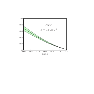
Figure 36: The unpolarized cross section (left) and the helicity correlation parameter $A_{LL}$ (right) for wide-angle Compton scattering at $s=11\,{\rm GeV}^{2}$ as a function of the scattering angle $\theta$ in the c.m. Both observables are evaluated at NLO with the Compton form factors shown in Fig. 35. The error bands are explained in the text.

The correlation parameter $K_{LS}$ between the helicity of the incoming photon and the transverse polarization of the outgoing proton is sensitive to the tensor form factor $R_{T}$. Assuming $\kappa_{\rm C}=\kappa_{\rm em}\approx 0.37$ the study [68] found values well in the range of 10%. With our default fit we find $K_{LS}$ at $s=11\,{\rm GeV}^{2}$ as small as $1\%$ for backward angles $\theta$ and yet smaller in the forward hemisphere. This can be traced back to the approximate cancellation of two terms in the expression for $K_{LS}$, one proportional to $R_{T}$ and the other to $R_{V}$, see eq. (397) in [19]. For this particular kinematics, the uncertainties on $R_{T}$ from our fits hence greatly amplify in the observable $K_{LS}$, which unlike $A_{LL}$ turns out to be strongly energy dependent.

8 Summary and outlook

We have developed a parameterization of valence quark GPDs at zero skewness which takes into account dynamically motivated correlations between their $x$ and $t$ dependence. At small $x$ their form is consistent with dominance of the leading meson trajectories known from Regge phenomenology. For large $t$ they incorporate the soft Feynman mechanism, where the struck quark has a virtuality of order $\Lambda\sqrt{|t|}$. Both analytically and numerically our distributions satisfy the Drell-Yan relation between the large-$x$ power behavior of parton distributions at $t=0$ and the large-$t$ power behavior of the associated elastic form factors. This holds for both $H_{v}^{q}$ and $E_{v}^{q}$ and is to be understood in the sense of effective powers describing the $x$ or $t$ dependence in a finite range of these variables. Key features of our functional ansatz for the GPDs are approximately invariant under DGLAP evolution, so that with an appropriate change of the free parameters this ansatz can be used for a reasonable range of scales $\mu$.

Good fits of the GPDs can be obtained to describe both the Dirac and Pauli form factors of proton and neutron, with an accuracy better than 20% for almost all data points and better than 5% in wide ranges of $t$. From $F_{1}^{p}$, where most data is available, we get a good determination of $H_{v}^{u}(x,t)$ up to $x\raisebox{-4.0pt}{$\,\stackrel{{\scriptstyle\textstyle<}}{{\sim}}\,$}0.8$. It is stable under a change of parameterization, provided we assume an exponential $t$ dependence as in (11). Under this assumption we have thus well determined the average squared impact parameter $\langle\mbox{\boldmath{$b$}}^{2}\rangle^{u}_{x}$ of $u$ quarks in the $x$ range just quoted. We have however seen that this does not suffice to fix the limiting behavior of $\langle\mbox{\boldmath{$b$}}^{2}\rangle^{u}_{x}$ for $x\to 1$. Given the paucity of data on $F_{1}^{n}$, the distribution $H_{v}^{d}(x,t)$ is less well determined, but we find clear indications that $\langle\mbox{\boldmath{$b$}}^{2}\rangle^{d}_{x}>\langle\mbox{\boldmath{$b$}}^{2}\rangle^{u}_{x}$ for larger values of $x$. This implies that with increasing $|t|$ the suppression of $d$ quarks compared with $u$ quarks becomes even stronger than in the forward parton densities at large $x$.

With the fit results for $H_{v}^{q}$ we also achieve a rather good description of the isovector axial form factor $F_{A}$ under the simplifying assumptions that sea quarks can be neglected and that the impact parameter distribution of valence quarks is independent of the quark helicity. With our ansatz for $\widetilde{H}_{v}^{q}$ we find that the largest uncertainty on the resulting form factor $F_{A}$ is due to the current errors on the polarized quark densities $\Delta d$ and $\Delta u$.

Using our ansatz for the proton helicity flip distributions we get good fits to the Pauli form factors $F_{2}^{p}$ and $F_{2}^{n}$. We find however considerable ambiguities in determining $E_{v}^{q}(x,t)$ since its forward limit is not known. The form factor data disfavor an identical shape in $x$ and $t$ of $E_{v}^{u}(x,t)$ and $E_{v}^{d}(x,t)$, but they have only little preference concerning the details of this flavor dependence. In particular, we cannot determine whether the forward limit $E_{v}^{u}(x,0)$ has a harder or a softer $x$ dependence than $E_{v}^{d}(x,0)$. Positivity constraints prove to be extremely valuable in constraining $E_{v}^{u}$ and $E_{v}^{d}$, as they severely restrict their size for $x\raisebox{-4.0pt}{$\,\stackrel{{\scriptstyle\textstyle>}}{{\sim}}\,$}0.5$ as well as their $t$ dependence. We find that, despite the uncertainties on these distributions, their moments $\int{\rm d}x\,xE_{v}^{q}(x,t)$ are reasonably well determined within our ansatz. With Ji’s angular momentum sum rule, the resulting valence quark contribution to the orbital angular momenta $\langle L^{u}\rangle$ and $\langle L^{d}\rangle$ have even smaller relative errors for the allowed range of our parameters.

The $x$ moments of our extracted GPDs are in reasonable agreement with results from lattice QCD, given the uncertainties of both our phenomenological determination and of the lattice calculations. With our results we have also calculated the distribution in the transverse plane of valence quarks with momentum fraction $x$, both in an unpolarized and in a transversely polarized proton. We have thus shown that “proton tomography” as proposed in [23, 24] is feasible on the basis of experimental data. Finally, we have used our GPDs to evaluate the form factors needed in the soft handbag approach to wide-angle Compton scattering, as well as the associated experimental observables. From a number of indicators we conclude that consistency of this approach requires momentum transfers $-t$ above $3\,{\rm GeV}^{2}$ or so.

Where can further progress be made? High-quality data on the neutron form factors in a wide $t$ range would be highly valuable for pinning down the differences in the spatial distribution of $u$ and $d$ quarks. Our fit results indicate in fact drastic differences in the behavior of $u$ and $d$ contributions to the form factors, which should be tested experimentally. The fit to the Pauli form factors suggests that the $t$ behavior of $F_{2}^{p}$ will continue to change beyond $5.5\,{\rm GeV}^{2}$, and it would be good to see whether this is indeed the case. Since Dirac and Pauli form factors are most natural to connect with the physics of parton distributions, we encourage experimenters to provide data on the Sachs form factors $G_{M}$ and $G_{E}$ at equal values of $t$ and with correlated errors wherever possible. Only then can one transform to $F_{1}$ and $F_{2}$ without introducing further theoretical bias or having to guess errors. With the available data on the axial form factor $F_{A}$ we could only take a glimpse at the role of quark helicity. More data on this fundamental quantity (in the form of data points rather than dipole parameterizations whenever possible) should lead to important progress in the study of $\widetilde{H}^{q}$. An improved determination of the polarized forward densities $\Delta q$ is under way at several experimental facilities and will also be of benefit to this study. For a more precise study of wide-angle Compton scattering, progress is required in the theory of power-suppressed contributions. Together with ongoing and planned measurements this should lead to an improved understanding of the dynamics and, if the soft handbag approach is further validated, eventually to pinning down the relevant form factors.

The fits to the electromagnetic form factors in this work have restricted us to zero skewness and to the valence quark sector. The ansatz we have developed for GPDs at $\xi=0$ can be used as an input for modeling distributions at nonzero $\xi$, using the concept of double distributions as shown e.g. in [80]. A nontrivial interplay between $t$ and the longitudinal variables can readily be implemented in this framework [81, 18]. Interesting observations concerning this formalism for proton distributions have recently been made in [82], building on earlier work in [83, 84]. Most of the exclusive processes where GPDs at nonzero $\xi$ occur are sensitive to sea quarks and also to gluons, in particular the important channels of deeply virtual Compton scattering and of neutral vector meson production. It will be interesting to investigate the dynamical interplay between the quark singlet and gluons in the impact parameter distributions, similarly to what has been seen for the distributions in momentum fraction $x$. In some channels, like the production of pseudoscalar mesons or pion pairs, one can however selectively probe the valence quark combinations of GPDs, see Sect. 1 of [18] and Sect. 5 of [19]. This opens the possibility to investigate the transverse distribution of valence quarks at small $x$, where elastic form factors have only a limited reach. The versatility of the GPD formalism and vigorous experimental activity let us hope that important progress is still to come.

Appendix A Details on form factor data

Experimental data are usually given for the magnetic and electric form factors $G_{E}$ and $G_{M}$, or for their ratio. Natural quantities for our parameterization of GPDs and their physical interpretation are the Dirac and Pauli form factors, so that we must perform the conversion

$$F_{1}=\frac{G_{E}+\tau G_{M}}{1+\tau},\qquad\qquad\qquad F_{2}=\frac{G_{M}-G_{E}}{1+\tau},$$ (90)

where $\tau=-t/(4m^{2})$. To obtain central values for $F_{1}$ and $F_{2}$ is rather straightforward, but we could not derive errors on these quantities in a rigorous way, lacking information on the correlation between the errors on $G_{E}$ and $G_{M}$. We encourage experimentalists to provide correlated errors on the two form factors (or derived quantities) whenever possible, since depending on the physical context one or the other set of form factors is more adequate.

For the proton form factors we have used the results from [85], where the original data from [41, 86, 87] was reanalyzed using the additional information on the ratio $G_{E}/G_{M}$ measured by the recoil polarization method in [88, 76]. With increasing $t$ the measurements using this method deviate from those obtained with a Rosenbluth separation, which is affected by QED radiative corrections growing with $t$ (see [70] and references therein).

To obtain $F_{1}^{p}$ we have used the central values and errors on $G_{M}^{p}$ together with the analytic parameterization for $G_{E}^{p}/G_{M}^{p}$ given in [85]. In calculating errors on $F_{1}$ we have only used the errors on $G_{M}$ but not those on the parameterization of $G_{E}/G_{M}$. The uncertainty on $G_{E}/G_{M}$ is included in the errors on the reanalyzed $G_{M}$ data given in [85], and counting it again in the conversion (90) would not be consistent. In discarding them we obtain the same relative errors on $F_{1}^{p}$ as those on $G_{M}$. They are between $0.8\%$ and $2.4\%$ for $-t\leq 10\,{\rm GeV}^{2}$ and then grow up to $9\%$ at the highest $t$ of the data. If we had added the errors on the parameterization of $G_{E}/G_{M}$ in quadrature, the resulting errors on $F_{1}^{p}$ would have been increased by at most a factor of 1.5 for $-t\leq 7.7\,{\rm GeV}^{2}$. (Beyond this value the ratio $G_{E}/G_{M}$ is taken as zero in [85] and it is unclear which error one should assign to it.)

For $F_{2}^{p}$ we have used the analytic parameterization of $G_{M}^{p}$ given in [85] together with the data and errors on $G_{E}^{p}/G_{M}^{p}$ measured with the recoil polarization method in [88, 76, 89]. For calculating the errors on $F_{2}$ we have used those on $G_{E}/G_{M}$ but not those on the parameterization of $G_{M}$ (which overestimate the experimental errors on $G_{M}$ in the $t$ range we need). If we were to add in quadrature an error on $G_{M}$ of $1.5\%$ for $-t<1\,{\rm GeV}^{2}$ and of $2\%$ otherwise, our errors on $F_{2}^{p}$ would increase by at most a factor of 1.6. The recoil data only go down to $-t=0.32\,{\rm GeV}^{2}$, and in order to have some data for lower $-t$ we have also included the results of [90] for $G_{M}$ and $G_{E}$ obtained by a Rosenbluth separation, using (90) and adding the errors on $G_{M}$ and $G_{E}$ in quadrature. The values for $F_{2}^{p}$ we obtain from these data match rather well with those from the recoil measurements in the $t$ region where they overlap (see Fig. 17), indicating that in the kinematics of interest the two methods are reasonably consistent. The errors we estimate for $F_{2}^{p}$ are between $1\%$ and $4\%$, with the exception of two data points with $5\%$ and one point with $7\%$.

For the neutron form factors we have restricted ourselves to results published after 1990 and only considered values of $t$ where data for both $G_{M}^{n}$ and $G_{E}^{n}$ are available, adding their errors in quadrature (as well as statistical, systematic and theoretical errors when they are given separately). The measurements in [61, 62] cover a range $0.5\,{\rm GeV}^{2}\leq-t\leq 1.5\,{\rm GeV}^{2}$, and we obtain $F_{1}^{n}$ with errors between 6% and 17% and $F_{2}^{n}$ with errors between $0.8\%$ and $2.4\%$. At $-t=0.255\,{\rm GeV}^{2}$ we have combined the measurement of $G_{M}^{n}$ from [59] and the one of $G_{E}^{n}$ from [60]. The resulting error on $F_{2}^{n}$ is 5%, whereas we obtain $F_{1}^{n}=-0.010\pm 0.035$ with a huge error. This is because the individual terms $G_{E}^{n}=0.066\pm 0.037$ and $\tau G_{M}^{n}=-0.077\pm 0.003$ in (90) nearly cancel. We nevertheless keep this data point, since a $\chi^{2}$ fit to the data will correctly take into account its large uncertainty. At the high-$t$ end we have taken data from [91]. We do not use their results at $-t=1.75\,{\rm GeV}^{2}$ and $2.5\,{\rm GeV}^{2}$ since the central values of $(G_{E}^{n})^{2}$ came out negative. From the remaining points $-t=3.25\,{\rm GeV}^{2}$ and $4\,{\rm GeV}^{2}$ we obtained $F_{1}^{n}$ with errors around 30% and $F_{2}^{n}$ with errors around 20%.

To have an indication of how well our fits describe proton data in the lower and upper range of available $t$, we give in App. B separate values of $\chi^{2}$ for data sets labeled “low” and “high” as specified in Table 3.

Table 3: Details of the data sets for which separate values of $\chi^{2}$ are given in the tables of App. B.

data set	references	data points	range of $-t/\,{\rm GeV}^{2}$
$F_{1}^{p}$ low	[41, 86]	49	$0.156$ to $7$
$F_{1}^{p}$ high	[87]	13	$2.862$ to $31.2$
$F_{1}^{n}$	[59, 60, 61, 62, 91]	8	$0.255$ to $4$
$F_{1}$ total		70
$F_{2}^{p}$ low	[90]	18	$0.0389$ to $1.75$
$F_{2}^{p}$ high	[76, 88, 89]	28	$0.32$ to $5.54$
$F_{2}^{n}$	[59, 60, 61, 62, 91]	8	$0.255$ to $4$
$F_{2}$ total		54

Appendix B Details of fit results

In the Tables of this section we list the results of the various fits discussed in this paper. We have performed $\chi^{2}$ fits to the form factor data using the minimization package Minuit [92]. The $1\,\sigma$ errors on the parameters are defined by the contour in parameter space for which

$$\chi^{2}=\chi^{2}_{\rm min}+\Delta\chi^{2},$$ (91)

where $\Delta\chi^{2}$ corresponds to a confidence level of 68%. One respectively has $\Delta\chi^{2}=2.30$, $3.53$, $4.72$ for 2, 3, 4 free parameters in the fit. The error bands shown in our figures have been derived from the $1\,\sigma$ errors on the fitted parameters by standard error propagation (see e.g. Sect. 31.2 of [32]). This takes properly into account correlations between errors on different parameters, which are typically quite large in our fits.

Our default fit for $H_{v}^{q}$ is specified in Sect. 3.2 and listed in the first row of Table 8, and our default fit for $E_{v}^{q}$ is explained in Sect. 5.3 and shown in Table 13. The covariance and error correlation matrices of these fits are given in Tables 4 and 5, respectively. All our fits for $E_{v}^{q}$ use the exponential ansatz (55) with the profile function (59) and the forward limit (65). Except for Table 14 we have fixed $\alpha=0.55$ in all fits. No error is given on $C_{u}$ when a fit has chosen its maximum value $1.22\,{\rm GeV}^{-2}$ allowed by the positivity constraint (63).

Table 4: The covariance matrix (left) and correlation matrix (right) of the default fit to $H_{v}^{q}$ described in Sect. 3.2 and listed in the first row of Table 8. The entries of the covariance matrix are in units of $\,{\rm GeV}^{-4}$ and are normalized such that diagonal elements give the squared $1\,\sigma$ errors on a parameter.

	$B_{q}$	$A_{u}$	$A_{d}$
$B_{q}$	$\phantom{-}6.95\cdot 10^{-4}$	$-4.84\cdot 10^{-4}$	$\phantom{-}5.69\cdot 10^{-3}$
$A_{u}$	$-4.84\cdot 10^{-4}$	$\phantom{-}6.11\cdot 10^{-4}$	$-1.38\cdot 10^{-3}$
$A_{d}$	$\phantom{-}5.69\cdot 10^{-3}$	$-1.38\cdot 10^{-3}$	$\phantom{-}8.22\cdot 10^{-2}$

	$B_{q}$	$A_{u}$	$A_{d}$
$B_{q}$	$\phantom{-}1$	$-0.743$	$\phantom{-}0.750$
$A_{u}$	$-0.743$	$\phantom{-}1$	$-0.194$
$A_{d}$	$\phantom{-}0.750$	$-0.194$	$\phantom{-}1$

Table 5: The covariance matrix (left) and correlation matrix (right) of the default fit to $E_{v}^{q}$ described in Sect. 5.3 and listed in Table 13. The entries of the covariance matrix are in units of $\,{\rm GeV}^{-4}$ and are normalized such that diagonal elements give the squared $1\,\sigma$ errors on a parameter.

	$\beta_{u}$	$D_{u}$	$D_{d}$
$\beta_{u}$	$\phantom{-}5.01\cdot 10^{-2}$	$-2.15\cdot 10^{-2}$	$-8.24\cdot 10^{-3}$
$D_{u}$	$-2.15\cdot 10^{-2}$	$\phantom{-}1.17\cdot 10^{-2}$	$\phantom{-}1.80\cdot 10^{-3}$
$D_{d}$	$-8.24\cdot 10^{-3}$	$\phantom{-}1.80\cdot 10^{-3}$	$\phantom{-}2.84\cdot 10^{-3}$

	$\beta_{u}$	$D_{u}$	$D_{d}$
$\beta_{u}$	$\phantom{-}1$	$-0.884$	$-0.693$
$D_{u}$	$-0.884$	$\phantom{-}1$	$\phantom{-}0.311$
$D_{d}$	$-0.693$	$\phantom{-}0.311$	$\phantom{-}1$

In Tables 6 to 16 we give the fitted parameters and their $1\,\sigma$ errors. For the sake of legibility we have omitted the units of $A_{q}$, $B_{q}$, $C_{q}$, $D_{q}$ and $\alpha^{\prime}$, which are always taken as $\,{\rm GeV}^{-2}$. The columns labeled “low” and “high” give the $\chi^{2}$ per number of data points for the separate proton data sets specified in Table 3, and the columns “$p$” and “$n$” give the corresponding numbers for the combined proton data and for the neutron data. The column “total” gives the $\chi^{2}$ per degrees of freedom, which is the quantity minimized in the fit. Note that if different fits in the same table have different numbers of free parameters, then the normalization of $\chi^{2}/\mathrm{d.o.f.}$ differs slightly from one row to another. The precise $\chi^{2}$ values should be interpreted with care because of the inadequacies affecting our errors on the Dirac and Pauli form factors (see App. A). This applies in particular to the low-$t$ data on $F_{1}^{p}$, whose errors are particularly small. To assess the quality of a fit it is hence useful to consider in addition to its $\chi^{2}$ also the “pull” as shown in Figures 7 and 20.

From Table 3 it is clear that the low-$t$ data on $F_{1}^{p}$ tend to dominate the $\chi^{2}$ minimization in the fit to the Dirac form factor because of the large number of data points. This could be circumvented by reweighting the $\chi^{2}$ for different data points, but we have opted for the more straightforward procedure without weights, given that our best fit turns out to describe the large-$t$ data on $F_{1}^{p}$ and the data on $F_{1}^{n}$ quite well. In a similar fashion, the proton data tend to dominate over those for the neutron in the fits to both the Dirac and the Pauli form factors due to the paucity of neutron data.

Table 6: Fits to $H_{v}^{q}(x,t)=q_{v}(x)\exp[tf_{q}(x)]$ using the CTEQ6M parton densities at scale $\mu=2\,{\rm GeV}$ and $f_{q}(x)=\alpha^{\prime}(1-x)^{n-1}\log(1/x)+(A_{q}-\alpha^{\prime})(1-x)^{n}$ from (23) and (27). More information on the different columns is given in the text.

	fit parameters			$\chi^{2}/$data points				$\chi^{2}/\mathrm{d.o.f.}$
$n$	$\alpha^{\prime}$	$A_{u}$	$A_{d}$	low	high	$p$	$n$	total
1	$1.38\pm 0.01$	$0.070\pm 0.006$	$0.25\pm 0.04$	1.42	0.60	1.25	1.55	1.34
2	$1.08\pm 0.02$	$0.78\pm 0.01$	$1.05\pm 0.05$	4.48	8.79	5.39	2.22	5.25

Table 7: Fits to $H_{v}^{q}(x,t)=q_{v}(x)\exp[tf_{q}(x)]$ using the CTEQ6M parton densities at $\mu=2\,{\rm GeV}$ and $f_{q}(x)=\alpha^{\prime}(1-x)^{2}\log(1/x)+B_{q}(1-x)^{2}+A_{q}\,x(1-x)$ from (28) with fixed $\alpha^{\prime}=0.9\,{\rm GeV}^{-2}$.

fit parameters			$\chi^{2}/$data points				$\chi^{2}/\mathrm{d.o.f.}$
$B_{u}=B_{d}$	$A_{u}$	$A_{d}$	low	high	$p$	$n$	total
$0.43\pm 0.02$	$0.164\pm 0.014$	$1.35\pm 0.21$	3.05	1.75	2.77	2.15	2.82
$0.32\pm 0.01$	$0.190\pm 0.009$		4.23	1.64	3.69	9.46	4.47

Table 8: Fits to $H_{v}^{q}(x,t)=q_{v}(x)\exp[tf_{q}(x)]$ using the CTEQ6M parton densities at $\mu=2\,{\rm GeV}$ and $f_{q}(x)=\alpha^{\prime}(1-x)^{3}\log(1/x)+B_{q}(1-x)^{3}+A_{q}\,x(1-x)^{2}$ from (29) with fixed $\alpha^{\prime}=0.9\,{\rm GeV}^{-2}$.

fit parameters				$\chi^{2}/$data points				$\chi^{2}/\mathrm{d.o.f.}$
$B_{u}$	$B_{d}$	$A_{u}$	$A_{d}$	low	high	$p$	$n$	total
$0.59\pm 0.03$		$1.22\pm 0.02$	$2.59\pm 0.29$	2.27	0.70	1.94	1.12	1.93
$0.59\pm 0.03$	$0.32\pm 0.14$	$1.26\pm 0.04$	$3.82\pm 0.78$	1.78	1.32	1.68	0.73	1.67
$0.56\pm 0.02$	$0.75\pm 0.08$	$1.17\pm 0.03$		3.22	0.76	2.70	2.36	2.78
$0.50\pm 0.01$		$1.20\pm 0.02$		2.98	0.69	2.50	9.24	3.36

Table 9: Fits to $H_{v}^{q}(x,t)=q_{v}(x)\exp[tf_{q}(x)]$ with $f_{q}(x)$ as in Table 8 and different sets of CTEQ6M parton distributions at $\mu=2\,{\rm GeV}$.

	fit parameters			$\chi^{2}/$data points				$\chi^{2}/\mathrm{d.o.f.}$
set	$B_{u}=B_{d}$	$A_{u}$	$A_{d}$	low	high	$p$	$n$	total
17	$0.55\pm 0.03$	$1.21\pm 0.02$	$2.52\pm 0.30$	1.79	1.23	1.68	1.09	1.68
18	$0.64\pm 0.03$	$1.24\pm 0.02$	$2.60\pm 0.27$	2.96	0.58	2.46	1.30	2.44
35	$0.58\pm 0.03$	$1.25\pm 0.03$	$2.88\pm 0.28$	2.20	0.72	1.89	0.98	1.86
36	$0.59\pm 0.03$	$1.22\pm 0.03$	$2.85\pm 0.29$	1.99	0.91	1.77	0.81	1.73

Table 10: Fits to $H_{v}^{q}(x,t)=q_{v}(x)\exp[tf_{q}(x)]$ with $f_{q}(x)=\alpha^{\prime}(1-x)^{3}\log(1/x)+B_{q}(1-x)^{3}+A_{q}\,x(1-x)^{2}$ from (29) and CTEQ6M parton densities taken at different scales $\mu$.

	fit parameters				$\chi^{2}/$data points				$\chi^{2}/\mathrm{d.o.f.}$
$\mu$	$\alpha^{\prime}$	$B_{u}=B_{d}$	$A_{u}$	$A_{d}$	low	high	$p$	$n$	total
1 GeV	$1.17\pm 0.05$	$0.50\pm 0.12$	$1.81\pm 0.07$	$2.62\pm 0.31$	1.16	0.70	1.06	1.11	1.13
2 GeV	$0.97\pm 0.04$	$0.43\pm 0.09$	$1.32\pm 0.06$	$2.51\pm 0.35$	1.77	1.53	1.72	0.86	1.72
4 GeV	$0.89\pm 0.03$	$0.36\pm 0.08$	$1.10\pm 0.06$	$2.58\pm 0.38$	2.23	2.09	2.20	0.89	2.17
8 GeV	$0.84\pm 0.03$	$0.29\pm 0.07$	$0.96\pm 0.06$	$2.71\pm 0.41$	2.56	2.42	2.53	1.10	2.51

Table 11: Fits to $H_{v}^{q}(x,t)=q_{v}(x)\,(1-tf_{q}(x)/p)^{-p}$ with $f_{q}(x)$ as in Table 10 and the CTEQ6M parton densities at $\mu=2\,{\rm GeV}$.

	fit parameters				$\chi^{2}/$data points				$\chi^{2}/\mathrm{d.o.f.}$
$p$	$\alpha^{\prime}$	$B_{u}=B_{d}$	$A_{u}$	$A_{d}$	low	high	$p$	$n$	total
$\infty$	$0.97\pm 0.04$	$\phantom{-}0.43\pm 0.09$	$1.32\pm 0.06$	$2.51\pm 0.35$	1.77	1.53	1.72	0.86	1.72
4	$0.91\pm 0.06$	$\phantom{-}0.84\pm 0.17$	$2.28\pm 0.14$	$4.48\pm 0.50$	1.06	0.85	1.02	1.25	1.11
3	$0.96\pm 0.09$	$\phantom{-}0.66\pm 0.25$	$3.34\pm 0.22$	$6.11\pm 0.59$	0.92	0.70	0.87	1.64	1.02
2.5	$1.21\pm 0.14$	$-0.12\pm 0.39$	$5.38\pm 0.42$	$8.75\pm 0.73$	0.81	0.44	0.73	2.18	0.95
2	$2.73\pm 0.18$	$-6.44\pm 0.74$	$21.0\pm 2.3$	$27.3\pm 2.7$	1.34	6.19	2.36	4.14	2.72

Table 12: Fits for $E_{v}^{q}$ with free parameters $D_{u}$, $D_{d}$ and $C_{u}$, $C_{d}$ subject to the constraint (63). In all fits $C_{d}$ takes it maximum allowed value $2.59\,{\rm GeV}^{-2}$. Further explanations on the fits for $E_{v}^{q}$ are given in the text.

		fit parameters			$\chi^{2}/$data points				$\chi^{2}/\mathrm{d.o.f.}$
$\beta_{u}$	$\beta_{d}$	$D_{u}$	$D_{d}$	$C_{u}$	low	high	$p$	$n$	total
4	5	$\phantom{-}0.38\pm 0.12$	$-0.65\pm 0.13$	$1.22$	1.89	0.89	1.28	0.83	1.32
5	5	$\phantom{-}0.14\pm 0.07$	$-0.65\pm 0.05$	$0.85\pm 0.14$	2.03	0.90	1.34	0.79	1.36
6	5	$-0.06\pm 0.06$	$-0.65\pm 0.05$	$0.60\pm 0.13$	2.13	0.94	1.40	0.76	1.41
4	6	$\phantom{-}0.38\pm 0.07$	$-0.82\pm 0.04$	$1.22$	1.94	0.87	1.29	0.79	1.31
5	6	$\phantom{-}0.14\pm 0.07$	$-0.82\pm 0.04$	$0.82\pm 0.14$	2.03	0.91	1.35	0.76	1.36
6	6	$-0.05\pm 0.10$	$-0.82\pm 0.12$	$0.58\pm 0.46$	2.14	0.94	1.41	0.74	1.41

Table 13: Fit for $E_{v}^{q}$ with fixed parameters $C_{u}=1.22\,{\rm GeV}^{-2}$, $C_{d}=2.59\,{\rm GeV}^{-2}$ and $\beta_{d}-\beta_{u}=1.60$.

fit parameters			$\chi^{2}/$data points				$\chi^{2}/\mathrm{d.o.f.}$
$\beta_{u}$	$D_{u}$	$D_{d}$	low	high	$p$	$n$	total
$3.99\pm 0.22$	$0.38\pm 0.11$	$-0.75\pm 0.05$	1.92	0.88	1.29	0.80	1.31

Table 14: Four-parameter fits for $E_{v}^{q}$ with equal values of the parameters for $u$ and $d$ quarks. In the fit of the first row the constraint $C_{q}\leq 1.22\,{\rm GeV}^{-2}$ from positivity is imposed, whereas in the fit of the second row $C_{q}$ is left completely free.

fit parameters				$\chi^{2}/$data points				$\chi^{2}/\mathrm{d.o.f.}$
$\alpha$	$\beta_{u}=\beta_{d}$	$D_{u}=D_{d}$	$C_{u}=C_{d}$	low	high	$p$	$n$	total
$0.53\pm 0.02$	$7.56\pm 1.95$	$-0.59\pm 0.31$	$1.22$	4.48	1.01	2.37	13.26	4.30
$0.61\pm 0.05$	$2.24\pm 0.71$	$\phantom{-}0.04\pm 0.17$	$3.50\pm 1.04$	3.87	0.80	2.00	13.27	3.97

Table 15: Fits for $E_{v}^{q}$ with free parameters $D_{u}=D_{d}$ and $C_{u}$, $C_{d}$ subject to the constraint (63).

		fit parameters			$\chi^{2}/$data points				$\chi^{2}/\mathrm{d.o.f.}$
$\beta_{u}$	$\beta_{d}$	$D_{u}=D_{d}$	$C_{u}$	$C_{d}$	low	high	$p$	$n$	total
7	5	$-0.41\pm 0.02$	$1.22$	$1.61\pm 0.25$	2.79	0.84	1.61	3.38	1.98
8	5	$-0.49\pm 0.02$	$1.00\pm 0.25$	$1.78\pm 0.28$	2.63	0.91	1.58	1.88	1.72
9	5	$-0.56\pm 0.02$	$0.60\pm 0.20$	$2.16\pm 0.31$	2.58	0.96	1.60	1.15	1.62
10	5	$-0.63\pm 0.02$	$0.29\pm 0.16$	$2.48\pm 0.32$	2.55	1.06	1.64	0.76	1.60

Table 16: Fits for $E_{v}^{q}$ with free parameters $\beta_{u}$, $\beta_{d}$, $D_{u}$, $D_{d}$ and $C_{u}=C_{d}$. In all fits $C_{q}$ takes its maximum value $1.22\,{\rm GeV}^{-2}$ allowed by the constraint (63).

fit parameters				$\chi^{2}/$data points				$\chi^{2}/\mathrm{d.o.f.}$
$\beta_{u}$	$\beta_{d}$	$D_{u}$	$D_{d}$	low	high	$p$	$n$	total
$8.97\pm 2.86$	$6.75\pm 1.82$	$-0.62\pm 0.34$	$-0.72\pm 0.27$	2.34	1.36	1.75	2.93	2.12
$9.54\pm 1.79$	$6.49\pm 1.27$	$-0.69\pm 0.20$		2.38	1.35	1.75	2.93	2.08
$7.76\pm 1.23$		$-0.47\pm 0.18$	$-0.85\pm 0.16$	2.24	1.47	1.77	3.15	2.13
$8.42\pm 1.30$		$-0.74\pm 0.16$		3.57	1.11	2.08	15.9	4.36

References

- [1] X. D. Ji, Phys. Rev. Lett. 78, 610 (1997) [hep-ph/9603249].
- [2] A. V. Radyushkin, Phys. Rev. D 56, 5524 (1997) [hep-ph/9704207].
- [3] J. C. Collins and A. Freund, Phys. Rev. D 59, 074009 (1999) [hep-ph/9801262].
- [4] A. V. Radyushkin, Phys. Rev. D 58, 114008 (1998) [hep-ph/9803316].
- [5] M. Diehl, T. Feldmann, R. Jakob and P. Kroll, Eur. Phys. J. C 8, 409 (1999) [hep-ph/9811253].
- [6] D. Müller, D. Robaschik, B. Geyer, F. M. Dittes and J. Hořejši, Fortsch. Phys. 42, 101 (1994) [hep-ph/9812448].
- [7] J. Blümlein, B. Geyer and D. Robaschik, Phys. Lett. B 406, 161 (1997) [hep-ph/9705264].
- [8] M. Göckeler et al. [QCDSF Collaboration], Phys. Rev. Lett. 92, 042002 (2004) [hep-ph/0304249].
- [9] P. Hägler et al. [LHPC and SESAM Collaborations], Phys. Rev. D 68, 034505 (2003), hep-lat/0304018.
- [10] P. Hägler et al. [LHPC and SESAM Collaborations], hep-lat/0312014.
- [11] J. W. Negele et al., Nucl. Phys. Proc. Suppl. 128, 170 (2004) [hep-lat/0404005].
- [12] V. Y. Petrov, P. V. Pobylitsa, M. V. Polyakov, I. Börnig, K. Goeke and C. Weiss, Phys. Rev. D 57, 4325 (1998) [hep-ph/9710270].
- [13] M. Penttinen, M. V. Polyakov and K. Goeke, Phys. Rev. D 62, 014024 (2000) [hep-ph/9909489].
- [14] S. Scopetta and V. Vento, Phys. Rev. D 69, 094004 (2004) [hep-ph/0307150].
- [15] B. Pasquini, M. Traini and S. Boffi, hep-ph/0407228.
- [16] S. J. Brodsky, M. Diehl and D. S. Hwang, Nucl. Phys. B 596, 99 (2001) [hep-ph/0009254].
- [17] M. Diehl, T. Feldmann, R. Jakob, and P. Kroll, Nucl. Phys. B 596, 33 (2001), Erratum-ibid. B 605, 647 (2001), [hep-ph/0009255].
- [18] K. Goeke, M. V. Polyakov and M. Vanderhaeghen, Prog. Part. Nucl. Phys. 47, 401 (2001) [hep-ph/0106012].
- [19] M. Diehl, Phys. Rept. 388, 41 (2003) [hep-ph/0307382].
- [20] J. Pumplin et al. [CTEQ collaboration], JHEP 0207, 012 (2002) [hep-ph/0201195].
- [21] J. Blümlein and H. Böttcher, Nucl. Phys. B 636, 225 (2002) [hep-ph/0203155].
- [22] M. Burkardt, Phys. Rev. D 62, 071503 (2000), Erratum-ibid. D 66, 119903 (2002), [hep-ph/0005108].
- [23] J. P. Ralston and B. Pire, Phys. Rev. D66, 111501 (2002) [hep-ph/0110075].
- [24] M. Burkardt, Int. J. Mod. Phys. A 18, 173 (2003) [hep-ph/0207047].
- [25] Jefferson Lab Collaboration E-99-114, Spokespersons C. Hyde-Wright, A. Nathan, B. Wojtsekhowski.
- [26] F. Olness et al., hep-ph/0312323.
- [27] D. H. Beck and R. D. McKeown, Ann. Rev. Nucl. Part. Sci. 51, 189 (2001) [hep-ph/0102334].
- [28] M. Diehl, Eur. Phys. J. C 25, 223 (2002), Erratum-ibid. C 31, 277 (2003), [hep-ph/0205208].
- [29] M. Burkardt and G. A. Miller, hep-ph/0312190.
- [30] S. Liuti and S. K. Taneja, hep-ph/0405014.
- [31] P. V. Landshoff, J. C. Polkinghorne and R. D. Short, Nucl. Phys. B 28, 225 (1971).
- [32] K. Hagiwara et al. [Particle Data Group], Phys. Rev. D 66, 010001 (2002).
- [33] K. Igi and P. Kroll, Phys. Lett. B 218, 95 (1989).
- [34] A. V. Barnes et al., Phys. Rev. Lett. 37, 76 (1976).
- [35] V. N. Gribov, hep-ph/0006158.
- [36] M. Burkardt, hep-ph/0105324.
- [37] M. Burkardt, Phys. Lett. B 595 (2004) 245 [hep-ph/0401159].
- [38] S. J. Brodsky, T. Huang, and G. P. Lepage, in: Particles and Fields 2, Procs. of the Banff Summer Institute, Banff, Alberta, 1981, Eds. A. Z. Capri and A. N. Kamal (Plenum, New York, 1981) p. 143.
- [39] J. Bolz and P. Kroll, Z. Phys. A 356, 327 (1996) [hep-ph/9603289].
- [40] C. Vogt, Phys. Rev. D 63, 034013 (2001) [hep-ph/0007277].
- [41] T. Janssens et al., Phys. Rev. 142, 922 (1966)
- [42] M. Beneke and T. Feldmann, Nucl. Phys. B 685 (2004) 249 [hep-ph/0311335].
- [43] J. C. Collins, L. Frankfurt and M. Strikman, Phys. Rev. D 56, 2982 (1997) [hep-ph/9611433].
- [44] T. Becher, R. J. Hill and M. Neubert, Phys. Rev. D 69, 054017 (2004) [hep-ph/0308122].
- [45] A. H. Mueller, Phys. Rept. 73, 237 (1981).
- [46] F. Yuan, Phys. Rev. D 69, 051501 (2004) [hep-ph/0311288].
- [47] G. P. Lepage and S. J. Brodsky, Phys. Rev. D 22 (1980) 2157.
- [48] A. Peterman, Phys. Rept. 53, 157 (1979).
- [49] M. Burkardt, Phys. Lett. B 582, 151 (2004) [hep-ph/0309116].
- [50] S. D. Drell and T. M. Yan, Phys. Rev. Lett. 24, 181 (1970).
- [51] P. Hoodbhoy, X. D. Ji and F. Yuan, Phys. Rev. Lett. 92, 012003 (2004) [hep-ph/0309085].
- [52] M. Diehl, T. Feldmann, P. Kroll and C. Vogt, Phys. Rev. D 61, 074029 (2000) [hep-ph/9912364].
- [53] T. Kitagaki et al., Phys. Rev. D 28 (1983) 436.
- [54] V. Bernard, L. Elouadrhiri and U. G. Meissner, J. Phys. G 28, R1 (2002) [hep-ph/0107088].
- [55] A. Airapetian et al. [HERMES Collaboration], Phys. Rev. Lett. 92, 012005 (2004) [hep-ex/0307064].
- [56] R. L. Jaffe, hep-ph/9602236.
- [57] A. V. Belitsky, X. D. Ji and F. Yuan, Phys. Rev. D 69, 074014 (2004) [hep-ph/0307383].
- [58] P. V. Pobylitsa, Phys. Rev. D 66, 094002 (2002) [hep-ph/0204337].
- [59] P. Markowitz et al., Phys. Rev. C 48, 5 (1993).
- [60] T. Eden et al., Phys. Rev. C 50, 1749 (1994).
- [61] G. Warren et al. [Jefferson Lab E93-026 Collaboration], Phys. Rev. Lett. 92, 042301 (2004) [nucl-ex/0308021].
- [62] R. Madey et al. [E93-038 Collaboration], Phys. Rev. Lett. 91, 122002 (2003) [nucl-ex/0308007].
- [63] X. D. Ji, J. Phys. G 24, 1181 (1998) [hep-ph/9807358].
- [64] Y. Goto et al. [Asymmetry Analysis Collaboration], Phys. Rev. D 62, 034017 (2000) [hep-ph/0001046].
-
[65]
N. Mathur, S. J. Dong, K. F. Liu, L. Mankiewicz and N. C. Mukhopadhyay,
Phys. Rev. D 62, 114504 (2000)
[hep-ph/9912289];
V. Gadiyak, X. D. Ji and C. W. Jung, Phys. Rev. D 65, 094510 (2002) [hep-lat/0112040]. - [66] H. W. Huang and P. Kroll, Eur. Phys. J. C 17, 423 (2000) [hep-ph/0005318].
- [67] H. W. Huang, R. Jakob, P. Kroll and K. Passek-Kumerički, Eur. Phys. J. C 33, 91 (2004) [hep-ph/0309071].
- [68] H. W. Huang, P. Kroll and T. Morii, Eur. Phys. J. C 23 (2002) 301, Erratum-ibid. C 31 (2003) 279, [hep-ph/0110208].
- [69] H. W. Huang and T. Morii, Phys. Rev. D 68, 014016 (2003) [hep-ph/0305132].
- [70] Y. C. Chen, A. Afanasev, S. J. Brodsky, C. E. Carlson and M. Vanderhaeghen, hep-ph/0403058.
- [71] I. V. Anikin, B. Pire and O. V. Teryaev, Phys. Rev. D 62, 071501 (2000) [hep-ph/0003203].
- [72] A. V. Radyushkin and C. Weiss, Phys. Rev. D 63, 114012 (2001) [hep-ph/0010296].
- [73] C. W. Bauer, S. Fleming, D. Pirjol and I. W. Stewart, Phys. Rev. D 63 (2001) 114020 [hep-ph/0011336].
- [74] M. Beneke, A. P. Chapovsky, M. Diehl and T. Feldmann, Nucl. Phys. B 643 (2002) 431 [hep-ph/0206152].
- [75] M. Beneke and T. Feldmann, Nucl. Phys. B 592 (2001) 3 [hep-ph/0008255].
- [76] O. Gayou et al. [Jefferson Lab Hall A Collaboration], Phys. Rev. Lett. 88, 092301 (2002) [nucl-ex/0111010].
- [77] M. Diehl, T. Feldmann, H. W. Huang and P. Kroll, Phys. Rev. D 67, 037502 (2003) [hep-ph/0212138].
- [78] M. Diehl, T. Feldmann, R. Jakob and P. Kroll, Phys. Lett. B 460, 204 (1999) [hep-ph/9903268].
- [79] G. A. Miller, Phys. Rev. C 69, 052201 (2004) [nucl-th/0402092].
- [80] I. V. Musatov and A. V. Radyushkin, Phys. Rev. D 61, 074027 (2000) [hep-ph/9905376].
- [81] L. Mankiewicz, G. Piller and A. Radyushkin, Eur. Phys. J. C 10, 307 (1999) [hep-ph/9812467].
- [82] B. C. Tiburzi, hep-ph/0405211.
- [83] M. V. Polyakov and C. Weiss, Phys. Rev. D 60, 114017 (1999) [hep-ph/9902451].
- [84] O. V. Teryaev, Phys. Lett. B 510, 125 (2001) [hep-ph/0102303].
- [85] E. J. Brash, A. Kozlov, S. Li and G. M. Huber, Phys. Rev. C 65 (2002) 051001 [hep-ex/0111038].
-
[86]
C. Berger, V. Burkert, G. Knop, B. Langenbeck and K. Rith,
Phys. Lett. B 35 (1971) 87;
W. Bartel et al., Nucl. Phys. B 58 (1973) 429;
R. C. Walker et al., Phys. Rev. D 49 (1994) 5671;
J. Litt et al., Phys. Lett. B 31 (1970) 40;
L. Andivahis et al., Phys. Rev. D 50, 5491 (1994). - [87] A. F. Sill et al., Phys. Rev. D 48 (1993) 29.
-
[88]
M. K. Jones et al. [Jefferson Lab Hall A Collaboration],
Phys. Rev. Lett. 84, 1398 (2000)
[nucl-ex/9910005];
O. Gayou et al. [Jefferson Lab Hall A Collaboration], Phys. Rev. C 64, 038202 (2001). - [89] B. D. Milbrath et al. [Bates FPP Collaboration], Phys. Rev. Lett. 80, 452 (1998), Erratum-ibid. 82, 2221 (1999) [nucl-ex/9712006].
- [90] L. E. Price, J. R. Dunning, M. Goitein, K. Hanson, T. Kirk and R. Wilson, Phys. Rev. D 4, 45 (1971).
- [91] A. Lung et al., Phys. Rev. Lett. 70, 718 (1993).
- [92] F. James and M. Roos, Comput. Phys. Commun. 10, 343 (1975).