Single top production and decay at next-to-leading order

Abstract

We present the results of a next-to-leading order analysis of single top production including the decay of the top quark. Radiative effects are included both in the production and decay stages, using a general subtraction method. This calculation gives a good treatment of the jet activity associated with single top production. We perform an analysis of the single top search at the Tevatron, including a consideration of the main backgrounds, many of which are also calculated at next-to-leading order.

I Introduction

Following the discovery of the top quark at the Tevatron in Run I Abe:1994st ; Abe:1995hr ; Abachi:1995iq , one of the aims of the current round of data-taking is to study the top quark in more detail. In addition to the accumulation of further statistics in the $t\bar{t}$ pair-production channel, both collaborations are performing a search for single top production Juste:2004an ; Abbott:2000pa ; Abazov:2001ns ; Acosta:2004er ; Acosta:2001un . Since single top production proceeds by the exchange (or production) of a $W$ boson, it offers another window into the weak interactions of the top quark and potentially can lead to a direct measurement of $V_{tb}$. Relative to the $t\bar{t}$ pair-production channel, single top production is suppressed by the weak coupling but favored by phase space.

We shall report here on the method of inclusion of single top processes into the general next-to-leading order Monte Carlo program MCFM Campbell:1999ah ; Campbell:2000bg ; Campbell:2002tg and give phenomenological results relevant to the search strategy in Run II. At the Born level the single top processes which we include are the $s$-channel process Cortese:fw ; Stelzer:1995mi ; Heinson:1996zm ,

$$u+{\bar{d}}\rightarrow W^{*}\rightarrow t+{\bar{b}},$$ (1)

the $t$-channel process Willenbrock:cr ; Yuan:1989tc ; Ellis:1992yw ; Carlson:1993dt ; Heinson:1996zm ,

$$b+u\rightarrow t+d,$$ (2)

and the $tW$ mode Tait:1999cf ; Belyaev:2000me ,

$$b+g\rightarrow t+W^{-}.$$ (3)

At the Tevatron, the $tW$ mode, Eq. (3), evaluated in the Born approximation represents less than one percent of the total single top cross section; in this paper we will not consider it further. The processes shown in Eqs. (1-3) are schematic. The actual implementation in the program includes a sum over all contributing partons in the initial state. In addition, we also include the leptonic decay of the top quark,

$$t\rightarrow\nu+e^{+}+b,$$ (4)

which allows a better comparison with experimental studies.

Although some information can be extracted from Born-level calculations, the first serious approximation in QCD is obtained by including $O(\alpha_{S})$ radiative corrections. We shall refer to this as next-to-leading order, (NLO). It is only in NLO that a calculation gives any information about the choice of factorization and renormalization scale. Moreover, if the calculation includes jets in the final state, it is only in NLO that one obtains first information about the structure of the jets. The NLO corrections to the inclusive $s$-channel mode have been presented in ref. Smith:1996ij and the corrections to the inclusive $t$-channel process have been considered in ref. Bordes:1994ki ; Stelzer:1997ns . The NLO corrections to the differential distributions for the production of single top, (without the decay of the top quark), which are needed for comparison with experimental results, have first been considered in ref. Harris:2002md for the processes in Eqs. (1) and (2). For a recent update of this work see ref. Sullivan:2004ie .

In this paper we extend this program by adding the leptonic decay of the top quark with full spin correlations, as noted above, and also by including the effects of gluon radiation in the decay. The approximations employed in incorporating the QCD corrections are described in Section II.

Section III outlines the calculation of the $O(\alpha_{\mathrm{s}})$ corrections to the decay of a free top quark which is helpful to establish notation. The subtraction method which we use to include the radiative corrections to the decay of a top quark in the single top production processes is described in Section IV.

The search for single top is expected to be more challenging than top-antitop associated production, both because of the smaller cross section and the presence of larger backgrounds. We therefore give a full account of the signal and background processes in Section V. Both the signal and the dominant background processes are evaluated at next-to-leading order.

II QCD corrections

In order to describe the inclusion of radiative corrections we shall discuss the $s$-channel process. The diagrams for the $t$-channel process can easily be constructed by crossing. They are obtained by reading the diagrams shown in Figs. 1-6 from bottom to top, instead of from left to right. Some of the statements made below are specific to the $s$-channel process, but the extensions to the $t$-channel process are obvious.

We shall work in the on-shell approximation for the top quark. Thus every diagram considered has one top quark exactly on its mass shell. Diagrams without an on-shell top quark are suppressed by $\Gamma_{t}/m_{t}$ where $\Gamma_{t}$ and $m_{t}$ are the width and mass of the top quark. In this approximation the real radiative corrections fall into three types: radiation associated with the initial state (Fig. 1), radiation in the final state associated with the production of the top quark (Fig. 2), and radiation in the final state associated with the decay of the top quark (Fig. 3). The double bars in these figures indicate which top quark is on its mass shell. By producing the top quark strictly on its mass shell we are assured that the diagrams in Figs. 2 and 3 are separately gauge invariant.

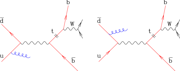
Figure 1: Initial-state radiation in the production stage.

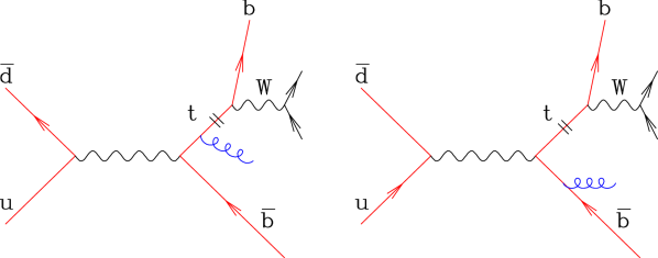
Figure 2: Final-state radiation in the production stage.

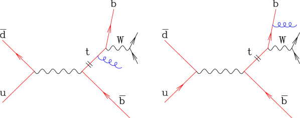
Figure 3: Final-state radiation in the decay stage.

In addition to these real radiation diagrams we also have virtual radiation diagrams. In our approximation these again fall into the same three categories; virtual radiation in the initial state Fig. 4, final-state virtual radiation in the production stage Fig. 5, and final-state virtual radiation in the decay stage, Fig. 6. Self energy contributions on massless external lines have not been displayed. They give rise to scaleless integrals, which are set equal to zero in the dimensional regularization scheme.

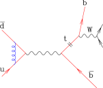
Figure 4: Virtual radiation in the initial state.

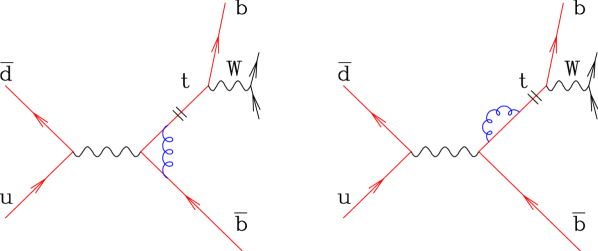
Figure 5: Final-state virtual radiation in the production stage.

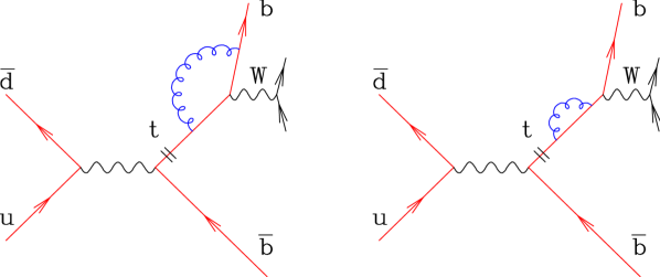
Figure 6: Final-state virtual radiation in the decay stage.

We have neglected the interference between real radiation in production and decay diagrams. An example is shown in Fig. 7. We also neglect the virtual radiation diagrams that link the production and decay stages, Fig. 8.

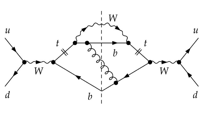
Figure 7: Interference between radiation in production and decay, real terms.

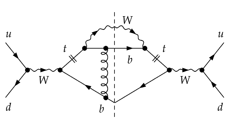
Figure 8: Interference between radiation in production and decay, virtual terms

The physical reason for the neglect of these diagrams has been provided in Refs. Fadin:1993kt ; Fadin:1993dz ; Melnikov:np . The characteristic time scale for the production of the $t{\bar{b}}$ pair is of order $1/m_{t}$ while the time for the decay is $1/\Gamma_{t}$. Therefore in general, radiation in the production and decay stages are separated by a large time and the interference effects average to zero. The potentially dangerous region for this argument is the one in which the emitted gluon is soft since this effect is not confined to a time of order $1/m_{t}$. The phase space for soft radiation is limited by the region in which the propagators remain resonant and the gluon energy is less than of order $\Gamma_{t}$. However because of the cancellation of real and virtual radiation the region of soft radiation is not especially privileged. Thus for infrared safe variables these interference effects are expected to be of order $\alpha_{\mathrm{s}}\Gamma_{t}/m_{t}$.

Confirmation of this suppression for the $s$-channel process is provided by the work of Pittau Pittau:1996rp , who included interference between the decay and production stages. The final results are consistent with an effect of order $\Gamma/m_{t}$. A similar study has been performed for $e^{+}e^{-}\rightarrow t{\bar{t}}$ including the subsequent decay of the top quarks Macesanu:2001bj . Here the effect of nonfactorizable corrections in the invariant mass distribution of the top was found to be very small.

The implementation of the cancellation of soft and collinear radiation contributions which are separately divergent is performed using the subtraction method Ellis:1980wv . In our program MCFM, we have consistently used the dipole subtraction method for massless particles as developed by Catani and Seymour Catani:1996jh ; Catani:1997vz . For the case of single top production we have a massive quark in the final state, so we have implemented a generalization of this scheme as suggested in Catani:2002hc . A useful further generalization has been suggested by Nagy and Trócsányi Nagy:1998bb ; Nagy:2003tz , who introduced a tunable parameter $\alpha$ which controls the size of the subtraction region. We have extended the massive results of ref. Catani:2002hc to include this parameter. Further details may be found in Appendix A.

In order to deal with radiation in the decay stage of the process we have developed a specialized subtraction procedure, which we discuss in Section IV. We expect that this method may be useful in other contexts. In particular, it could be applied to the decay of the top quarks in the $t\bar{t}$ production process.

III Radiative corrections to top decay

One of the new results in this paper is the inclusion of the QCD corrections to the decay of a top quark in a Monte Carlo program. Since the phase space for the decay of an on-shell top quark factorizes from the production phase space, most of the features of the full calculation are present in the decay of an isolated top quark. For simplicity, and in order to introduce the notation, we first reproduce the well-known result for radiation from a free top quark Jezabek:1988iv .

The lowest order process is $t(p_{t})\rightarrow W(p_{W})+b(p_{b})$, where the momenta carried by the fields are shown in brackets. The matrix element summed and averaged over initial spin and color is,

$$\overline{\sum}|{{\cal M}}_{0}|^{2}=2\frac{G_{F}}{\sqrt{2}}m_{t}^{4}(1-r^{2})(1+2r^{2})\;.$$ (5)

where we have defined $r^{2}=(p_{t}-p_{b})^{2}/m_{t}^{2}$. For the case of an on-shell $W$ boson, $r^{2}=M_{W}^{2}/m_{t}^{2}$. Here and throughout this paper, the mass of the $b$-quark is set equal to zero. The corresponding Born-approximation width is given by,

$$\Gamma_{0}=\frac{G_{F}m_{t}^{3}}{8\pi\sqrt{2}}(1-r^{2})^{2}(1+2r^{2})$$ (6)

III.1 Virtual corrections

The form-factor for the process $t\rightarrow W+b$ including virtual gluon corrections is defined by,

$$\Gamma^{\mu}(p_{b},p_{t})=\bar{u}(p_{b})F^{\mu}(p_{b},p_{t})u(p_{t})$$ (7)

with a massless $b$ quark and a massive $t$ quark and momentum transfer $p_{W}=p_{t}-p_{b}$. The contributing diagrams are shown in Fig. 9.

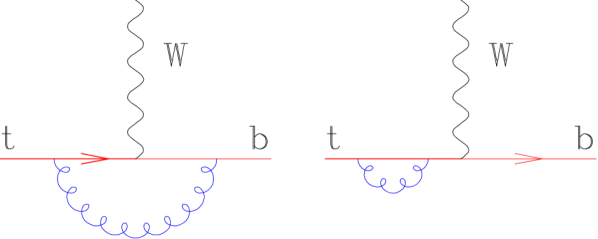
Figure 9: Virtual radiation in free top decay

The result for the form factor evaluated through order $\alpha_{\mathrm{s}}$ is well known Gottschalk:1980rv ; Schmidt:1995mr ; Harris:2002md ,

$$F^{\mu}(p_{b},p_{t}) = \gamma^{\mu}\gamma_{L}\Big{[}1+\frac{\alpha_{S}\;C_{F}}{4\pi\Gamma(1-\epsilon)}\Big{(}\frac{4\pi\mu^{2}}{m_{t}^{2}-i\varepsilon}\Big{)}^{\epsilon}C_{0}\Big{]}$$ (8)

$$+ \frac{\alpha_{S}\;C_{F}}{4\pi}\Big{[}C_{1}\frac{p_{b}^{\mu}}{m_{t}}\gamma_{R}+C_{2}\frac{p_{W}^{\mu}}{m_{t}}\gamma_{R}\Big{]}+O(\epsilon)$$

where

$$C_{0} = \Big{\{}-\frac{1}{\epsilon^{2}}-\frac{1}{\epsilon}\Big{(}\frac{5}{2}-2\ln(1-r^{2})\Big{)}-\frac{11+\eta}{2}-\frac{\pi^{2}}{6}-2\mathop{\mathrm{Li}}\nolimits_{2}(r^{2})$$

$$+ 3\ln(1-r^{2})-2\ln^{2}(1-r^{2})-\frac{1}{r^{2}}\ln(1-r^{2})\Big{\}}$$

$$C_{1} = \frac{2}{r^{2}}\ln(1-r^{2})$$ (9)

and

$$\gamma_{R/L}=\frac{1}{2}(1\pm\gamma_{5})\;.$$ (10)

The $C_{2}$ term will not contribute to physical amplitudes. The ultra-violet and infra-red divergences have been regulated by continuing to $d=4-2\epsilon$ dimensions. The dimensional regularization scheme is determined by the parameter $\eta$ as follows,

$$\eta = 1,\;\;\mbox{'t Hooft-Veltman scheme~{}\cite[cite]{\@@bibref{Authors Phrase1YearPhrase2}{'tHooft:1972fi}{\@@citephrase{(}}{\@@citephrase{)}}}}$$

$$\eta = 0,\;\;\mbox{four-dimensional helicity scheme~{}\cite[cite]{\@@bibref{Authors Phrase1YearPhrase2}{Bern:2002zk}{\@@citephrase{(}}{\@@citephrase{)}}}}\;.$$ (11)

The final result for the virtual correction to the total decay width is,

$$\Gamma_{\rm virtual}=\Gamma_{0}\;\frac{\alpha_{S}C_{F}}{2\pi\Gamma(1-\epsilon)}\left(\frac{4\pi\mu^{2}}{m_{t}^{2}}\right)^{\epsilon}\left(C_{0}+\frac{1}{2}C_{1}\frac{1-r^{2}}{1+2r^{2}}\right)+O(\epsilon)\;.$$ (12)

We now make three parenthetic remarks which are useful for including the virtual corrections in the production processes, Eqs. (1,2). First, we note that Eq. (9) is valid for $r^{2}<1$. For the case when $r^{2}>1$, which is needed for the virtual corrections to the $s$-channel production process, we apply the transformation,

$$\mathop{\mathrm{Li}}\nolimits_{2}(r^{2})=\frac{\pi^{2}}{6}-\mathop{\mathrm{Li}}\nolimits_{2}(1-r^{2})-\ln(1-r^{2})\ln r^{2}$$ (13)

and analytically continue by replacing $\ln(1-r^{2})$ with $\ln(1-r^{2}-i\varepsilon)$. Second, we note that the result for the light quark vertex including the virtual corrections, which is also needed for the case of production, is as follows Altarelli:1979ub ,

$$\Gamma^{\mu}(p_{d},p_{u})=\bar{u}(p_{d})\gamma^{\mu}\gamma_{L}u(p_{u})\;\Bigg{[}1+\frac{\alpha_{S}C_{F}}{4\pi\Gamma(1-\epsilon)}\Big{(}\frac{4\pi\mu^{2}}{-q^{2}-i\varepsilon}\Big{)}^{\epsilon}\Big{\{}-\frac{2}{\epsilon^{2}}-\frac{3}{\epsilon}-7-\eta+O(\epsilon)\Big{\}}\Bigg{]}$$ (14)

with $q=p_{u}-p_{d}$. Third, for the case of the production processes the singularities in these virtual corrections are canceled by equal and opposite singularities in the integrated dipoles. With a little work, using results for the integrated dipole terms in Appendix A, one can demonstrate this cancellation.

III.2 Real corrections

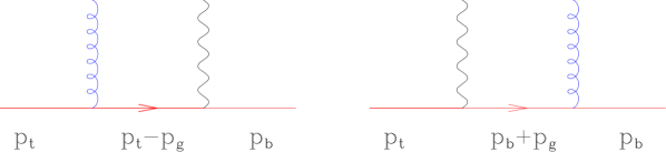
Figure 10: Real radiation in free top decay

The Feynman diagrams for the process

$$t(p_{t})\rightarrow b(p_{b})+W(p_{W})+g(p_{g})\;,$$ (15)

are shown in Fig. 10. The result for the matrix element squared in four dimensions is given as follows

$$\overline{\sum}|{{\cal M}}|^{2} = 2g^{2}C_{F}\frac{G_{F}}{\sqrt{2}}m_{t}^{2}\Bigg{[}m_{t}^{2}(1-r^{2})(1+2r^{2})\Big{(}2\frac{p_{t}.p_{b}}{p_{b}.p_{g}\;p_{t}.p_{g}}-\frac{m_{t}^{2}}{(p_{t}.p_{g})^{2}}\Big{)}$$ (16)

$$+ 8r^{2}+2\frac{(p_{t}.p_{g}-p_{b}.p_{g})^{2}}{p_{b}.p_{g}\;p_{t}.p_{g}}(1+2r^{2})\Bigg{]}\;.$$

Applying the substitutions

$$p_{b}\cdot p_{g} = \frac{m_{t}^{2}}{2}(1-r)^{2}y$$

$$p_{t}\cdot p_{g} = \frac{m_{t}^{2}}{2}(1-r^{2})(1-z)\;,$$ (17)

the four-dimensional matrix element becomes,

$$\overline{\sum}|{{\cal M}}|^{2} = g^{2}C_{F}\Bigg{\{}\Big{[}\frac{1}{p_{b}.p_{g}}\Big{(}\frac{2}{1-z}-1-z\Big{)}-\frac{m_{t}^{2}}{(p_{t}.p_{g})^{2}}\Big{]}\;\overline{\sum}|{{\cal M}}_{0}|^{2}$$ (18)

$$+ 8m_{t}^{2}\frac{G_{F}}{\sqrt{2}}\Big{[}\frac{y}{1-z}\Big{(}\frac{3}{(1+r)}-r^{2}+2r-\frac{5}{2}\Big{)}+\frac{(1+2r^{2})}{(1-z)}-1\Big{]}\Bigg{\}}$$

In the rest frame of the top we obtain the two particle phase space for the decay $t\rightarrow W+b$

$$d\Phi^{(2)}(p_{W},p_{b};p_{t}) = \frac{d^{n}p_{b}}{(2\pi)^{n-1}}\frac{d^{n}p_{W}}{(2\pi)^{n-1}}\;(2\pi)^{n}\;\delta^{n}(p_{t}-p_{W}-p_{b})\;\delta(p_{b}^{2})\;\delta(p_{W}^{2}-r^{2}m_{t}^{2})$$ (19)

$$= =\frac{(4\pi)^{2\epsilon}}{8\;(2\pi)^{2}}\frac{1}{(m_{t}^{2})^{\epsilon}}\;(1-r^{2})^{1-2\epsilon}d^{n-1}\Omega_{w}$$

The corresponding result in the rest frame of the top for the decay $t\rightarrow W+b+g$ is

$$d\Phi^{(3)}(p_{W},p_{b},p_{g};p_{t}) = \frac{(1-r^{2})(1-r)^{2-4\epsilon}}{32\;(2\pi)^{4}}\;\;\frac{(m_{t}^{2})^{1-2\epsilon}(4\pi)^{3\epsilon}}{\Gamma(1-\epsilon)}\;d^{n-1}\Omega_{w}$$ (20)

$$\times \int_{0}^{1}\;dz\;(r^{2}+z(1-r^{2}))^{-\epsilon}\;\int_{0}^{y_{max}}dy\;y^{-\epsilon}\;(y_{max}-y)^{-\epsilon}$$

where the upper integration limit $y_{max}$ is given by

$$y_{max}=\frac{(1+r)^{2}z(1-z)}{\Big{(}z+r^{2}(1-z)\Big{)}}.$$ (21)

Taking the ratio of Eqs. (20) and (19) we obtain the factorized form,

$$d\Phi^{(3)}(p_{W},p_{b},p_{g};p_{t}) = d\Phi^{(2)}(p_{W},p_{b};p_{t})\times\frac{(1-r)^{2}}{16\pi^{2}}\;\;\frac{(m_{t}^{2})^{1-\epsilon}(4\pi)^{\epsilon}}{\Gamma(1-\epsilon)}$$

$$\times \Big{(}\frac{1+r}{1-r}\Big{)}^{2\epsilon}\;\int_{0}^{1}\;dz\;(r^{2}+z(1-r^{2}))^{-\epsilon}\;\int_{0}^{y_{max}}dy\;y^{-\epsilon}\;(y_{max}-y)^{-\epsilon}$$

Values of the reduced integrals defined by

$$\Big{\langle}f(y,z)\Big{\rangle}=\Big{(}\frac{1+r}{1-r}\Big{)}^{2\epsilon}\int_{0}^{1}\;dz\;(r^{2}+z(1-r^{2}))^{-\epsilon}\;\int_{0}^{y_{max}}dy\;y^{-\epsilon}\;(y_{max}-y)^{-\epsilon}\;f(z,y)$$ (23)

are given in Table 1.

Table 1: Table of integrals defined by Eq. (23).

$\Big{\langle}\frac{1}{y}\frac{2}{(1-z)}\Big{\rangle}$	$\frac{1}{\epsilon^{2}}-\frac{2}{\epsilon}\ln(1-r^{2})+2\ln^{2}(1-r^{2})+2\mathop{\mathrm{Li}}\nolimits_{2}(1-r^{2})-\frac{5\pi^{2}}{6}+O(\epsilon)$
$\Big{\langle}\frac{1}{y}\Big{\rangle}$	$-\frac{1}{\epsilon}-3+2\ln(1-r^{2})+\frac{r^{2}}{(1-r^{2})}\ln r^{2}+O(\epsilon)$
$\Big{\langle}\frac{z}{y}\Big{\rangle}$	$-\frac{1}{2\epsilon}-\frac{(7-5r^{2})}{4(1-r^{2})}+\ln(1-r^{2})-\frac{r^{4}}{2(1-r^{2})^{2}}\ln r^{2}+O(\epsilon)$
$\Big{\langle}\frac{-2}{(1+r)^{2}}\frac{1}{(1-z)^{2}}\Big{\rangle}$	$\frac{1}{\epsilon}+2-\frac{2r^{2}}{1-r^{2}}\ln r^{2}-2\ln(1-r^{2})+O(\epsilon)$
$\Big{\langle}\frac{1}{(1+r)^{2}}\frac{1}{(1-z)}\Big{\rangle}$	$\frac{r^{2}\ln r^{2}}{(1-r^{2})^{2}}+\frac{1}{1-r^{2}}+O(\epsilon)$
$\Big{\langle}\frac{1}{(1+r)^{4}}\frac{y}{(1-z)}\Big{\rangle}$	$\frac{r^{2}(2+r^{2})}{2(1-r^{2})^{4}}\ln r^{2}+\frac{(1+5r^{2})}{4(1-r^{2})^{3}}+O(\epsilon)$
$\Big{\langle}(1-r)^{2}\Big{\rangle}$	$\frac{(r^{2}+1)}{2}+\frac{r^{2}}{1-r^{2}}\ln r^{2}+O(\epsilon)$

Using these integrals we can calculate the contribution to the total decay width from the real diagrams. The result is,

$$\Gamma_{\rm real} = \Gamma_{0}^{(d)}\;\frac{\alpha_{S}C_{F}}{2\pi\Gamma(1-\epsilon)}\left(\frac{4\pi\mu^{2}}{m_{t}^{2}}\right)^{\epsilon}\Bigg{(}\frac{1}{\epsilon^{2}}+\frac{1}{\epsilon}\left(\frac{5}{2}-2\ln(1-r^{2})\right)-\frac{5\pi^{2}}{6}+2\mathop{\mathrm{Li}}\nolimits_{2}(1-r^{2})$$

$$-5\ln(1-r^{2})+2\ln^{2}(1-r^{2})-\frac{2r^{2}(1+r^{2})(1-2r^{2})}{(1-r^{2})^{2}(1+2r^{2})}\ln r^{2}-\frac{2(7r^{4}-5r^{2}-4)}{(1+2r^{2})(1-r^{2})}+\frac{\eta}{2}\Bigg{)}$$

$$\;.$$ (24)

The $\eta$-dependence has been restored in this equation, so that Eq. (III.2) is valid also for the ’t Hooft Veltman scheme.

III.3 Result for the corrected width

Using the virtual corrections of Eq. (12) and the real corrections of Eq. (III.2) we can calculate the value of the top width at $O(\alpha_{S})$. We write the correction to the decay rate in the form

$$\Gamma=\Gamma_{0}+\alpha_{\mathrm{s}}\Gamma_{1}$$ (25)

Our result is in agreement with the $m^{2}_{b}/m^{2}_{t}\rightarrow 0$ limit of the original calculation in ref. Jezabek:1988iv ,

$$\frac{\alpha_{\mathrm{s}}\Gamma_{1}}{\Gamma_{0}} = -\frac{\alpha_{\mathrm{s}}}{2\pi}C_{F}\Bigg{[}\frac{2}{3}\pi^{2}+4\;\mathop{\mathrm{Li}}\nolimits_{2}(r^{2})-\frac{3}{2}-2\;\ln\Big{(}\frac{r^{2}}{1-r^{2}}\Big{)}+2\;\ln r^{2}\ln(1-r^{2})$$ (26)

$$- \frac{4}{3(1-r^{2})}+\frac{(22-34\;r^{2})}{9(1-r^{2})^{2}}\ln r^{2}+\frac{(3+27\ln(1-r^{2})-4\ln r^{2})}{9(1+2r^{2})}\Bigg{]}\;,$$

where $r=M_{W}/m_{t}$. For $r\sim 4/9$ the QCD correction amounts to

$$\frac{\alpha_{\mathrm{s}}\Gamma_{1}}{\Gamma_{0}}\approx-0.8\alpha_{\mathrm{s}}$$ (27)

which lowers the leading order result for the width by about 10%.

IV Factorization of singularities in top quark decay

We wish to construct a counter-term for the process

$$t\rightarrow W+b+g$$ (28)

which has the same soft and collinear singularities as the full matrix element. This counter-term takes the form of a lowest order matrix element multiplied by a function $D$ which describes the emission of soft or collinear radiation,

$$|{{\cal M}}(\ldots p_{t},p_{W},p_{b},p_{g})|^{2}\rightarrow|{{\cal M}}_{0}(\ldots p_{t},\tilde{p}_{W},\tilde{p}_{b})|^{2}\times D(p_{t}.p_{g},p_{b}.p_{g},m_{t}^{2},M_{W}^{2})\;,$$ (29)

In the region of soft emission, or in the region where the momenta $p_{g}$ and $p_{b}$ are collinear, the right hand side of Eq. (29) has the same singularity structure as the full matrix element. The lowest order matrix element ${\cal M}_{0}$ in Eq. (29) is evaluated for values of the momenta $p_{W}$ and $p_{b}$ modified to absorb the four-momentum carried away by the gluon, and subject to the momentum conservation constraint, $p_{t}\rightarrow{\tilde{p}_{W}}+\tilde{p}_{b}$. The modified momenta denoted by a tilde are also subject to the mass-shell constraints, ${\tilde{p}_{b}}^{2}=0$ and ${\tilde{p}_{W}}^{2}=p_{W}^{2}$. The latter condition is necessary in order that the rapidly varying Breit-Wigner function for the $W$ is evaluated at the same kinematic point in the counterterm and in the full matrix element. We define $\tilde{p}_{W}$ by a Lorentz transformation, ${\tilde{p}_{W}}^{\mu}=\Lambda^{\mu}_{\nu}p_{W}^{\nu}$ fixed in terms of the momenta $p_{W}$ and $p_{t}$. Because $\tilde{p}_{W}$ and $p_{W}$ are related by a Lorentz transformation the phase space for the subsequent decay of the $W$ is unchanged.

The general form of a Lorentz transformation in the plane of the vectors $p_{t}$ and $p_{W}$ is given by (${\tilde{p}_{W}}^{\mu}=\Lambda^{\mu}_{\nu}p_{W}^{\nu}$),

$$\Lambda^{\mu\nu} = g_{\mu\nu}+\frac{\sinh(x)}{\sqrt{(p_{t}\cdot p_{W})^{2}-p_{W}^{2}p_{t}^{2}}}\;\Big{(}p_{t}^{\mu}p_{W}^{\nu}-p_{W}^{\mu}p_{t}^{\nu}\Big{)}$$ (30)

$$+ \frac{\cosh(x)-1}{(p_{t}\cdot p_{W})^{2}-p_{W}^{2}p_{t}^{2}}\;\Big{(}p_{t}\cdot p_{W}\;(p_{t}^{\mu}p_{W}^{\nu}+p_{W}^{\mu}p_{t}^{\nu})-p_{W}^{2}\;p_{t}^{\mu}p_{t}^{\nu}-p_{t}^{2}\;p_{W}^{\mu}p_{W}^{\nu}\Big{)}$$

The transformed momentum of the $b$ quark is fixed by $\tilde{p}_{b}=p_{t}-\tilde{p}_{W}$. For the special case in which we impose the condition $\tilde{p}_{b}^{2}=(p_{t}-{\tilde{p}_{W}})^{2}=0$ we get

$$\sinh(x) = \frac{1}{2\;p_{t}^{2}p_{W}^{2}}\Big{[}-(p_{t}^{2}-p_{W}^{2})p_{t}\cdot p_{W}+(p_{t}^{2}+p_{W}^{2})\sqrt{(p_{t}\cdot p_{W})^{2}-p_{W}^{2}p_{t}^{2}}\;\Big{]}$$

$$\cosh(x) = \frac{1}{2\;p_{t}^{2}p_{W}^{2}}\Big{[}+(p_{t}^{2}+p_{W}^{2})p_{t}\cdot p_{W}-(p_{t}^{2}-p_{W}^{2})\sqrt{(p_{t}\cdot p_{W})^{2}-p_{W}^{2}p_{t}^{2}}\;\Big{]}$$ (31)

Acting on the vector $p_{W}$ the Lorentz transformation becomes

$$\tilde{p}_{W}=\alpha\;\big{(}p_{W}-\frac{p_{t}\cdot p_{W}}{p_{t}^{2}}p_{t}\big{)}+\beta\;p_{t}$$ (32)

where the constants are given by

$$\alpha = \frac{p_{t}^{2}-p_{W}^{2}}{2\sqrt{(p_{t}\cdot p_{W})^{2}-p_{W}^{2}p_{t}^{2}}}$$ (33)

$$\beta = \frac{p_{t}^{2}+p_{W}^{2}}{2p_{t}^{2}}$$ (34)

Eq. (32) makes it clear that, in the top rest frame, the transformation on $p_{W}$ is a Lorentz boost along the direction of the $W$.

The momenta of the decay products of the $W$ can similarly be obtained by the same Lorentz transformation, Eqs. (30,IV).

IV.1 Subtraction counterterm

From Eq. (III.2) we may write the phase space for the decay of an on-shell top quark as

$$d\Phi^{(3)}(p_{W},p_{b},p_{g};p_{t}) = d\Phi^{(2)}(p_{W},p_{b};p_{t})\int[dg(p_{t},p_{W},y,z)]$$ (35)

$$\equiv d\Phi^{(2)}({\tilde{p}_{W}},{\tilde{p}_{b}};p_{t})\int[dg(p_{t},{\tilde{p}_{W}},y,z)]$$

The equivalence in Eq. (35) follows from Eq. (19) because $d^{n-1}\Omega_{w}=d^{n-1}\Omega_{\tilde{w}}$ since $p_{W}$ and ${\tilde{p}_{W}}$ are related by a boost. From Eq. (III.2) we see that the phase space integral for the emitted gluon is given by,

$$[dg(p_{t},\tilde{p}_{W},y,z)] = \frac{(1-r)^{2}}{16\pi^{2}}\;\;(m_{t}^{2})^{(1-\epsilon)}\;\frac{(4\pi)^{\epsilon}}{\Gamma(1-\epsilon)}$$ (36)

$$\times \Big{(}\frac{1+r}{1-r}\Big{)}^{2\epsilon}\;\int_{0}^{1}\;dz\;(r^{2}+z(1-r^{2}))^{-\epsilon}\;\int_{0}^{y_{max}}dy\;y^{-\epsilon}\;(y_{max}-y)^{-\epsilon}$$

where $y$ and $z$ are given by Eq. (III.2). By extension of Eq. (18) we choose the counterterm to be,

$$D((p_{t}+p_{g})^{2},(p_{b}+p_{g})^{2},m_{t}^{2},M_{W}^{2})=g^{2}\mu^{2\epsilon}C_{F}\Bigg{[}\frac{1}{p_{b}.p_{g}}\Big{(}\frac{2}{(1-z)}-1-z-\eta\epsilon(1-z)\Big{)}-\frac{m_{t}^{2}}{(t.g)^{2}}\Bigg{]}$$ (37)

where the role of the parameter $\eta$ is defined in Eq. (III.1). Performing the integral using the results of Table 1, we obtain the following result for the integrated counterterm,

$$\int[dg(p_{t},\tilde{p}_{W},y,z)] \times D((p_{t}+p_{g})^{2},(p_{b}+p_{g})^{2},m_{t}^{2},M_{W}^{2})=$$ (38)

$$\frac{\alpha_{S}C_{F}}{2\pi}\;\frac{(4\pi\mu^{2})^{\epsilon}}{m_{t}^{2\epsilon}\Gamma(1-\epsilon)}\Big{[}\frac{1}{\epsilon^{2}}+\frac{1}{\epsilon}\Big{(}\frac{5}{2}-2\ln(1-r^{2})\Big{)}$$

$$+ \frac{25}{4}+\frac{1}{2}\Big{(}\frac{1}{(1-r^{2})^{2}}-\frac{8}{(1-r^{2})}+7\Big{)}\ln r^{2}+\frac{1}{2(1-r^{2})}$$

$$+ 2\mathop{\mathrm{Li}}\nolimits_{2}(1-r^{2})-\frac{5\pi^{2}}{6}-5\ln(1-r^{2})+2\ln^{2}(1-r^{2})+\frac{\eta}{2}\Big{]}$$

V Phenomenological studies

The method of the previous section has been implemented in the Monte Carlo program, MCFM, allowing us to make predictions for kinematic distributions of both signal and background events. Before proceeding to describe our results for jets and the decay products of the top, we present a number of results on total cross sections.

V.1 Total cross section

Tables 2 and 3 give total cross sections using recent parton distributions and the updated top quark mass Azzi:2004rc . The input parameters which we use throughout this phenomenological section are presented in Table 4.

Table 2: LO and NLO cross sections for single top-quark production at the Tevatron and LHC for $m_{t}=178$ GeV. The branching ratio for the decay of the top quark is not included. Cross sections are evaluated with CTEQ6L1 ($\alpha_{\mathrm{s}}(M_{Z})=0.130$) and CTEQ6M ($\alpha_{\mathrm{s}}(M_{Z})=0.118$) PDFs Pumplin:2002vw , and all scales set to $m_{t}$. The errors represent Monte Carlo statistics only.

Process	$\sqrt{s}$ [TeV]	$\sigma_{LO}$ [pb]	$\sigma_{NLO}$ [pb]
$s$-channel, $p\bar{p}$ ($t$)	1.96	0.270	0.405 $\pm$0.0003
$s$-channel, $pp$ ($t$)	14	4.26	6.06 $\pm$0.004
$s$-channel, $pp$ ($\bar{t}$)	14	2.58	3.76 $\pm$0.003
$t$-channel, $p\bar{p}$ ($t$)	1.96	0.826	0.924 $\pm$0.001
$t$-channel, $pp$ ($t$)	14	146.2	150.0 $\pm$0.2
$t$-channel, $pp$ ($\bar{t}$)	14	84.8	88.5 $\pm$0.1

Table 3: LO and NLO cross sections for single top-quark production at the Tevatron and LHC for $m_{t}=178$ GeV. The branching ratio for the decay of the top quark is not included. Cross sections are evaluated with the MRST2002 NLO PDF set Martin:2002aw with $\alpha_{\mathrm{s}}(M_{Z})=0.1197$, and all scales set to $m_{t}$. The errors represent Monte Carlo statistics only.

Process	$\sqrt{s}$ [TeV]	$\sigma_{LO}$ [pb]	$\sigma_{NLO}$ [pb]
$s$-channel, $p\bar{p}$ ($t$)	1.96	0.285	0.404 $\pm$0.0003
$s$-channel, $pp$ ($t$)	14	4.57	6.17 $\pm$0.004
$s$-channel, $pp$ ($\bar{t}$)	14	2.85	3.86 $\pm$0.003
$t$-channel, $p\bar{p}$ ($t$)	1.96	1.009	1.032 $\pm$0.001
$t$-channel, $pp$ ($t$)	14	160.1	154.4 $\pm$0.2
$t$-channel, $pp$ ($\bar{t}$)	14	96.9	92.4 $\pm$0.1

Table 4: Input parameters

$m_{t}=178.$ GeV	$\Gamma_{0}=1.651$ GeV
$M_{W}=80.4$  GeV	$\Gamma_{W}=2.06$ GeV
$M_{Z}=91.188$ GeV	$\Gamma_{Z}=2.49$ GeV
$G_{F}=1.16639\times 10^{-5}$ GeV-2	$\alpha^{-1}=132.351$
$g_{W}^{2}=0.42651$	$e^{2}=0.0949475$

We have not performed a full analysis of the theoretical errors on these predictions. It is important to remember that the results for the $t$-channel process depend on the $b$-quark parton distribution, which is calculated rather than measured. This is the source of the relatively large difference between the $t$-channel Tevatron cross sections in Tables 2 and 3, compared to the $s$-channel process which is dominated by well-constrained valence quark distributions.

We have also compared our leading order (LO) and next-to-leading order (NLO) results for the total cross sections (without radiation in the decay) at $\sqrt{s}=1.96$ and 14 TeV with the results in ref. Harris:2002md . With the appropriate modification of the input parameters, we find agreement with their results within the quoted errors.

We now investigate what effect the inclusion of QCD corrections in the decay of the top quark has on the total cross section. Radiation in the decay should not change the total cross section. However in a perturbative approach this means that the difference should be of higher order in $\alpha_{\mathrm{s}}$. Including QCD radiation effects only in the production, we obtain

$$\sigma B_{t\rightarrow b\nu e}\equiv\sigma B_{W\rightarrow\nu e}=\sigma_{(0)}B_{W\rightarrow\nu e}+\alpha_{\mathrm{s}}\sigma_{(1)}B_{W\rightarrow\nu e}$$ (39)

where $\sigma_{(0)}$ and $\sigma_{(1)}$ are the LO and NLO cross sections, because in this order the width $t\rightarrow bW$ is equal to the total width. When we also include radiative corrections to the decay, we use the radiatively corrected total width $\Gamma=\Gamma_{0}+\alpha_{\mathrm{s}}\Gamma_{1}$, cf. Eqs. (6,25),

$$\sigma B_{t\rightarrow b\nu e+X}=\sigma_{(0)}\frac{\Gamma_{0}B_{W\rightarrow\nu e}}{\Gamma}+\alpha_{\mathrm{s}}\sigma_{(1)}\frac{\Gamma_{0}B_{W\rightarrow\nu e}}{\Gamma}+\sigma_{(0)}\frac{\alpha_{\mathrm{s}}\Gamma_{1}B_{W\rightarrow\nu e}}{\Gamma}$$ (40)

The difference between these two expressions is of $O(\alpha_{\mathrm{s}}^{2})$ and is given by

$$\sigma B_{t\rightarrow b\nu e+X}-\sigma B_{t\rightarrow b\nu e} = \alpha_{\mathrm{s}}\sigma_{(1)}\frac{\Gamma_{0}B_{W\rightarrow\nu e}}{\Gamma}-\alpha_{\mathrm{s}}\sigma_{(1)}B_{W\rightarrow\nu e}$$ (41)

$$= -\alpha_{\mathrm{s}}^{2}\sigma_{(1)}\frac{\Gamma_{1}B_{W\rightarrow\nu e}}{\Gamma}$$

Table 5: Comparison of LO and NLO cross sections for single $t$-quark production at the Tevatron and LHC. The NLO calculation is performed both without including QCD effects in the decay ($\sigma B_{t\rightarrow b\nu e}$) and also when it is included ($\sigma B_{t\rightarrow b\nu e+X}$). The top quark mass is $m_{t}=178$ GeV and cross sections are evaluated using MRST2002 NLO PDFs with all scales set to $m_{t}$. The errors represent Monte Carlo statistics only. Note that the values of $\Gamma_{t}$ at LO and NLO are $1.6511$ GeV and $1.5077$ GeV respectively and the branching ratio of the $W$ into leptons is ${\rm Br}(W\rightarrow e\nu)=0.1104$. The differences in the rates are in good agreement with the formulae in Eq. (41).

Process	$\sqrt{s}$ [TeV]	$\sigma_{0}B_{t\rightarrow b\nu e}$ (fb)	$\sigma B_{t\rightarrow b\nu e}$ (fb)	$\sigma B_{t\rightarrow b\nu e+X}$ (fb)
$s$-channel, $p\bar{p}$ ($t$)	1.96	31.54 $\pm$0.01	44.64 $\pm$0.03	45.88 $\pm$0.03
$s$-channel, $pp$ ($t$)	14	503.9 $\pm$0.2	681.0 $\pm$0.4	698.7 $\pm$0.4
$t$-channel, $p\bar{p}$ ($t$)	1.96	111.34 $\pm$0.06	113.95 $\pm$0.12	113.96 $\pm$0.12
$t$-channel, $pp$ ($t$)	14	17690. $\pm$8	17048. $\pm$16	16975. $\pm$16.

As shown in Table 5 the numerical differences are less than $3\%$ for the $s$-channel process and less than $0.5\%$ for the $t$-channel process.

V.2 Signals and Backgrounds at NLO

We shall consider the signal for single top production to be the presence of a lepton, missing energy and two jets, one of which is tagged as a $b$-jet. In the case where we have two tagged jets, we choose the jet to be assigned to the top quark at random. For clarity, we shall describe the processes at the parton level choosing specific partons in the initial state. In our program we sum over all the species of partons present in the initial proton and antiproton. For reactions considered at NLO, there can also be additional partons in the final state. We use the Run II $k_{T}$-clustering algorithm to find jets, with a pseudo-cone of size $R=1.0$ Blazey:2000qt . The first reactions to consider are the two signal processes

$$\begin{array}[]{r c l}u+\bar{d}&\rightarrow&t+\bar{b}\\ &&\>\raisebox{5.59721pt}{\hbox to0.0pt{$|$\hss}}\!\rightarrow\nu+e^{+}+b\end{array}$$ (42)

and

$$\begin{array}[]{r c l}b+u&\rightarrow&t+d\\ &&\>\raisebox{5.59721pt}{\hbox to0.0pt{$|$\hss}}\!\rightarrow\nu+e^{+}+b\end{array}\;.$$ (43)

Note that we present numerical results for the processes shown in Eqs. (42,43), summed over species of initial partons, i.e. the production of a $t$-quark (rather than a $\bar{t}$) with the decay $t\rightarrow\nu+e^{+}+b+X$. Thus in a hypothetical experiment with equal perfect acceptances for electrons of both charges and for muons of both charges the signal (and background) will be four times bigger, (if we ignore possible signatures coming from $W\rightarrow\tau\nu_{\tau}$). Unless explicitly stated otherwise, our NLO results for the signal processes are calculated including QCD corrections in both the production and decay of the top quark.

The background processes which we consider are of several types. The irreducible backgrounds are,

$$\begin{array}[]{r c l}u+\bar{d}&\rightarrow&W^{+}+b+\bar{b}\\ &&\>\raisebox{5.59721pt}{\hbox to0.0pt{$|$\hss}}\!\rightarrow\nu+e^{+}\end{array}$$ (44)

$$\begin{array}[]{r c l}u+b&\rightarrow&W^{+}+d+b\\ &&\>\raisebox{5.59721pt}{\hbox to0.0pt{$|$\hss}}\!\rightarrow\nu+e^{+}\end{array}\;.$$ (45)

$$\begin{array}[]{r c l}u+\bar{d}&\rightarrow&W^{+}+Z\\ &&\>\raisebox{5.59721pt}{\hbox to0.0pt{$|$\hss}}\raisebox{-2.15277pt}{$|$}\phantom{W^{+}+}\!\>\raisebox{5.59721pt}{\hbox to0.0pt{$|$\hss}}\!\rightarrow b+\bar{b}\\ &&\>\raisebox{5.59721pt}{\hbox to0.0pt{$|$\hss}}\!\rightarrow\nu+e^{+}\end{array}$$ (46)

There are also backgrounds related to $t\bar{t}$ production which contribute to the $W+$ 2 jets process. The case where both top quarks decay leptonically,

$$\begin{array}[]{r c l}u+\bar{u}&\rightarrow&t+\bar{t}\\ &&\>\raisebox{5.59721pt}{\hbox to0.0pt{$|$\hss}}\raisebox{-2.15277pt}{$|$}\phantom{t+}\!\>\raisebox{5.59721pt}{\hbox to0.0pt{$|$\hss}}\!\rightarrow\bar{b}+e^{-}+\bar{\nu}\\ &&\>\raisebox{5.59721pt}{\hbox to0.0pt{$|$\hss}}\!\rightarrow\nu+e^{+}+b\end{array}$$ (47)

contributes if the electron, $e^{-}$ (or muon, $\mu^{-}$) fails the cuts. If one of the top quarks instead decays hadronically then there can also be a contribution when only two jets are observed, either because of merging or because the extra jets lie outside the acceptance (or both),

$$\begin{array}[]{r c l}u+\bar{u}&\rightarrow&t+\bar{t}\\ &&\>\raisebox{5.59721pt}{\hbox to0.0pt{$|$\hss}}\raisebox{-2.15277pt}{$|$}\phantom{t+}\!\>\raisebox{5.59721pt}{\hbox to0.0pt{$|$\hss}}\!\rightarrow\bar{b}+q+\bar{q}\\ &&\>\raisebox{5.59721pt}{\hbox to0.0pt{$|$\hss}}\!\rightarrow\nu+e^{+}+b\end{array}$$ (48)

A significant background process involves $W$ + two light jet production where one of the light quark jets fakes a $b$-quark,

$$\begin{array}[]{r c l}u+\bar{d}&\rightarrow&W^{+}+{\rm 2~{}jets}\\ &&\>\raisebox{5.59721pt}{\hbox to0.0pt{$|$\hss}}\!\rightarrow\nu+e^{+}\end{array}$$ (49)

Further backgrounds involve the mistagging of a $c$-quark as a $b$-quark,

$$\begin{array}[]{r c l}u+\bar{s}&\rightarrow&W^{+}+u+\bar{c}\\ &&\>\raisebox{5.59721pt}{\hbox to0.0pt{$|$\hss}}\!\rightarrow\nu+e^{+}\end{array}$$ (50)

$$\begin{array}[]{r c l}u+\bar{d}&\rightarrow&W^{+}+c+\bar{c}\\ &&\>\raisebox{5.59721pt}{\hbox to0.0pt{$|$\hss}}\!\rightarrow\nu+e^{+}\end{array}$$ (51)

$$\begin{array}[]{r c l}u+c&\rightarrow&W^{+}+d+c\\ &&\>\raisebox{5.59721pt}{\hbox to0.0pt{$|$\hss}}\!\rightarrow\nu+e^{+}\end{array}$$ (52)

Our estimation of the rates for these processes depends on the cuts shown in Table 6, which have been chosen to mimic those used in an actual Run II analysis Juste:2004an .

Table 6: Cuts for the single top analysis presented in this section.

Lepton $p_{T}$	$p_{T}^{e}>20$ GeV
Lepton pseudorapidity	$|\eta^{e}|<1.1$
Missing $E_{T}$	$\hbox to0.0pt{$\;\!\!\not$\hss}{E_{T}}>20$ GeV
Jet $p_{T}$	$p_{T}^{\mbox{jet}}>15$ GeV
Jet pseudorapidity	$|\eta^{\mbox{jet}}|<2.8$
Mass of $b+l+\nu$	$140<m_{bl\nu}<210$ GeV

As well as the normal jet and lepton cuts, we perform a cut on the missing transverse energy and the mass of the ‘$b+l+\nu$’-system, $m_{bl\nu}$. The missing transverse energy vector is the negative of the vector sum of the transverse energy of the observed jets and leptons. The mass of the putative top system is determined by reconstructing the $W$ and combining it with the tagged $b$-jet. In reconstructing the $W$ the longitudinal momentum of the neutrino is fixed by constraining the mass of the $e\nu$ system to be equal to $M_{W}$. The two solutions for the longitudinal momentum of the neutrino are,

$$p_{L}^{\nu}=\frac{1}{2|p_{T}^{e}|^{2}}\Big{[}p_{L}^{e}\;\big{(}M_{W}^{2}-M_{T}^{2}+2|p_{T}^{e}||p_{T}^{\nu}|\big{)}\pm E^{e}\;\sqrt{(M_{W}^{2}-M_{T}^{2})(M_{W}^{2}-m_{T}^{2}+4|p_{T}^{e}||p_{T}^{\nu}|)}\Big{]}$$ (53)

In this equation $p_{T}^{\nu}$ is the measured missing transverse energy and

$$M_{T}^{2}=(|p_{T}^{e}|+|p_{T}^{\nu}|)^{2}-(\vec{p}_{T}^{\;e}+\vec{p}_{T}^{\;\nu})^{2}$$ (54)

is the transverse mass of the $W$. We resolve the twofold ambiguity in $p_{L}^{\nu}$ by choosing the solution which gives the largest (smallest) neutrino rapidity for the $W^{+}(W^{-})$.

Our results are shown in Table 7.

Table 7: Cross sections for the Tevatron Run II ($p{\bar{p}}$, $\sqrt{s}=1.96$ TeV) in femtobarns, calculated with MRST2002 and using the renormalization and factorization scale $\mu$. The cross sections contain two jets, subject to the cuts of Table 6. Next-to-leading order cross sections are also shown, where known. The last column estimates the importance of signal and background processes by including nominal tagging and mistagging efficiencies, using the NLO cross section where possible.

Process	Scale $\mu$	$\sigma_{LO}$ [fb]	$\sigma_{NLO}$ [fb]	Efficiency	$\sigma$ [fb]
$s$-channel single top, Eq. (42)	$m_{t}$	10.3	11.7	$1-(1-\varepsilon_{b})^{2}$	7.4
$s$-channel (with decay radiation)	$m_{t}$	10.3	11.3	$1-(1-\varepsilon_{b})^{2}$	7.2
$t$-channel single top, Eq. (43)	$m_{t}$	38.8	29.4	$\varepsilon_{b}$	11.8
$t$-channel (with decay radiation)	$m_{t}$	38.8	26.6	$\varepsilon_{b}$	10.6
$Wb\bar{b}$, Eq. (44)	$M_{W}$	36.0	47.5	$1-(1-\varepsilon_{b})^{2}$	30.4
$W+bj$, Eq. (45)	$M_{W}/4$	26.5	-	$\varepsilon_{b}$	10.6
$WZ$, Eq. (46)	$M_{W}$	3.64	3.91	$1-(1-\varepsilon_{b})^{2}$	2.5
$t\bar{t}$, Eq. (47)	$m_{t}$	4.34	-	$2\times(1-(1-\varepsilon_{b})^{2})$	5.6
$t\bar{t}$, Eq. (48)	$m_{t}$	4.94	-	$1-(1-\varepsilon_{b})^{2}$	3.2
$W$+2 jet, Eq. (49)	$M_{W}$	5530.	7030.	$1-(1-f_{J})^{2}$	35.1
$u\bar{s}\rightarrow Wu\bar{c}$, Eq. (50)	$M_{W}$	324.	-	$f_{c}$	19.4
$Wc\bar{c}$, Eq. (51)	$M_{W}$	36.0	47.5	$1-(1-f_{c})^{2}$	5.5
$W+cj$, Eq. (52)	$M_{W}/4$	54.7	-	$f_{c}$	3.3

In this table we first show the cross sections calculated assuming a perfectly efficient detector, both at LO and NLO where possible. The column labeled ‘Efficiency’ gives the rescaling factor that should be applied in order to take account of experimental efficiencies and fake rates. To give some idea of the importance of the background processes, we have used the nominal (and perhaps optimistic) values of these quantities shown in Table 8 to obtain the final column of Table 7.

Table 8: Nominal efficiencies used throughout this section.

$b$-tagging efficiency	$\varepsilon_{b}=40\%$
$c$-mistagged as $b$	$f_{c}=6\%$
Jet fake rate	$f_{J}=0.25\%$

A strategy for searching for the single top processes at the Tevatron involves examining the $H_{T}$ distribution Juste:2004an , where $H_{T}$ is defined by,

$$H_{T}=|p_{T}(\mbox{lepton})|+|\hbox to0.0pt{$\;\!\!\not$\hss}{E}_{T}|+\sum|p_{T}(\mbox{jet})|\;.$$ (55)

In Fig. 11 we show the $H_{T}$ distributions of the signal and background processes described above, rescaled by the nominal efficiencies given in Table 8. As in the table, the NLO calculation is used wherever it is known and the signal processes include gluon radiation in the decay of the top quark. We see that the $H_{T}$ distribution is harder for the single top distributions, than all backgrounds, except those which involve top production (which are however, small).

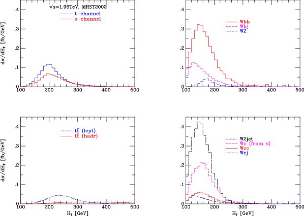
Figure 11: Predictions for $H_{T}$ showing single top signal, (top left), irreducible backgrounds (top right), $t\bar{t}$ backgrounds, (bottom left) and jet and charm fake rate (bottom right). Next-to-leading order estimates are used for the cross sections where available.

Despite this fact, one sees that the background rates are still large in the region of $H_{T}$ where the signal processes peak. This is demonstrated more clearly in Figure 12, where we show the $H_{T}$ distribution for the sum of all the backgrounds, the sum of the two single top processes and the total when combining signal and background. Although the single top signal represents about $50\%$ of the events in the bins of interest, an observation of this top production mechanism using the $H_{T}$ distribution is heavily reliant on accurate predictions of both the rates and shapes of the background processes. We stress that Figs. 11 and 12 depend on the particular values chosen for the efficiencies and will improve if better values are achieved.

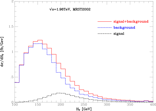
Figure 12: The $H_{T}$ distributions of signal, background and signal plus background. The curves correspond to the sum of the appropriate distributions shown in Figure 11.

A further quantity that may be used to discriminate between the $t$-channel signal process and backgrounds is $Q\eta$, where $Q$ is the charge of the lepton (in units of the positron charge) and $\eta$ is the pseudorapidity of the untagged jet. In this analysis Juste:2004an an additional cut is applied, requiring that one of the two jets must have a $p_{T}>30$ GeV. This extra cut serves to reduce the dominant backgrounds in Table 7 by $15$–$30\%$ whilst leaving the signal virtually unchanged. Since this is a targeted search for the $t$-channel process we have also rejected events with two tagged jets, since at leading order, Eq.(43) contains only one $b$-jet. Results for the $Q\eta$ distribution are shown in Fig. 13, demonstrating that the $t$-channel process is enhanced at large pseudorapidity compared to the backgrounds.

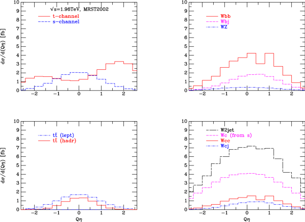
Figure 13: Predictions for $Q\eta$ showing single top signal, (top left), irreducible backgrounds (top right), $t\bar{t}$ backgrounds, (bottom left) and jet and charm fake rate (bottom right). Next-to-leading order estimates are used for the cross sections where available.

As before, even the pronounced effect observed in this distribution can be hidden when comparing the signal to the sum of all backgrounds, as shown in Fig. 14.

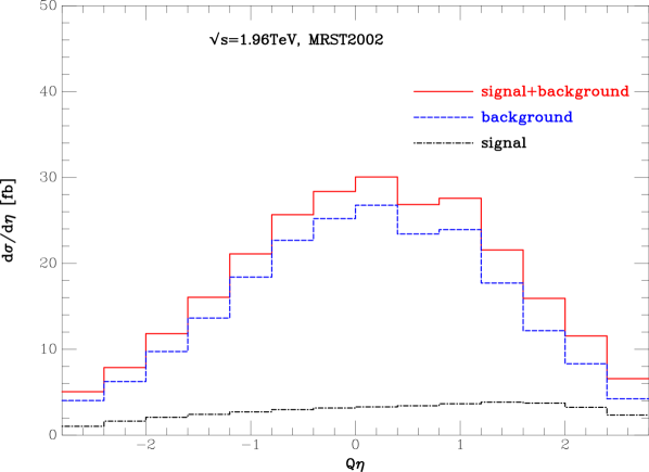
Figure 14: The $Q\eta$ distributions of signal, background and signal plus background. The curves correspond to the sum of the appropriate distributions shown in Figure 13.

Finally, we end this section with a comment on the effect of including the radiation in the top quark decay at NLO. We find that although the overall rate is lowered (cf. Table 7), the shapes of the $H_{T}$ and $Q\eta$ distributions are not altered significantly. This is demonstrated in Fig. 15, where we compare the $H_{T}$ ($s$-channel) and $Q\eta$ ($t$-channel) distributions with and without radiation in the decay. However this is a feature of our specific choice of cuts and we do not know this to be true in general.

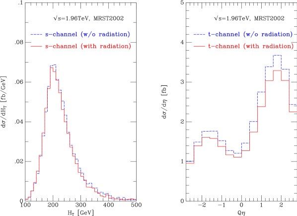
Figure 15: Comparison of the NLO distributions for $H_{T}$ in the $s$-channel process (left) and $Q\eta$ in the $t$-channel process (right), with and without radiation in decay.

VI Conclusions

We have presented the first results of our NLO Monte Carlo program which describes the signal and background for single top production. The new feature of our analysis is the inclusion of the decay of the top quark. Since our analysis is performed at next-to-leading order, we have included radiative effects both in the production and in the decay. Radiation in the decay is performed using a new subtraction method, which may be useful in other contexts.

We have studied the effects of the NLO corrections on two distributions that are relevant for single top searches at the Tevatron. The inclusion of the top quark decay is imperative for such an analysis for two reasons. Firstly, the cuts that are applied (in order to match the experimental analysis) are on the decay products and not on the top quark itself. Second, one of the distributions of interest, $H_{T}$, can only be calculated when the momenta of the decay products are known. We have also performed the calculation of a number of important backgrounds at NLO and examined the feasibility of using variables such as $H_{T}$ and $Q\eta$ to discriminate between the single top signal and the main backgrounds. We find that the inclusion of radiation in the decay makes very little difference in the shapes of these distributions, but further decreases the exclusive two-jet signal cross section. Our treatment is obviously approximate, because we assume $p_{T}$-independent efficiencies, stable $b$ and $c$ quarks and include no showering or hadronization. Nevertheless it confirms that the search for single top is extremely challenging and suggests that significantly larger tagging efficiencies and/or methods with greater discriminatory power will be needed to observe single top production. We hope to have contributed to this search by providing more reliable information on the kinematic structure of both the signal and the background.

Appendix A Integration of dipoles

As described in the text of the paper the production cross section was calculated using a subtraction method Ellis:1980wv . The particular subtraction terms were taken from ref. Catani:1997vz (CS) for the subtraction terms with massless particles and from ref. Catani:2002hc (CDST) for the dipoles involving massive particles in the final state.

In this appendix we describe two minor modifications of the methods in those references. The first is that we allow ourselves the freedom to work in the four-dimensional helicity scheme. This scheme has been used for the calculation of many virtual matrix elements, so we believe that our results may be useful in other contexts.

The second modification is that, following Nagy and Trócsányi Nagy:1998bb ; Nagy:2003tz we introduce a tuneable parameter $\alpha$ which can be used to reduce the range of integration over the singular variable. $\alpha=1$ corresponds to integration over the whole dipole phase space and for $\alpha<1$ the volume of phase space for the dipole subtraction is reduced. As detailed in Nagy:2003tz this serves a number of purposes. Since the subtraction is smaller, the mis-match between real matrix elements and subtractions is also reduced, leading to fewer events where the event and counter-event fall into different bins. In addition, for small $\alpha$ the counter-terms are only calculated in events where they actually play a role in canceling a singularity. This can lead to a saving in computer time. Lastly, the lack of $\alpha$-dependence in the results is a valuable check of the numerical implementation. For the massless case the integrations of the dipoles in reduced phase space volumes have been provided in Nagy:2003tz . The results for the $\alpha$ dependence of the massive dipoles are new.

To keep the appendix short we try and use a similar notation to refs. Catani:1997vz ; Catani:2002hc and refer back to specific equations in those references (CS Catani:1997vz and CDST Catani:2002hc ) when appropriate.

A.1 Initial-state emitter with initial state spectator

As explained above we have used a slight generalization of the dipole phase space (CS, Eq. (5.151)) where the variable ${\tilde{v}_{i}}$ is modified by the factor $\Theta(\alpha-{\tilde{v}}_{i})$. The variable ${\tilde{v}_{i}}$ is the rescaled value of the propagator, defined as

$${\tilde{v}_{i}}=\frac{p_{a}p_{i}}{p_{a}p_{b}}$$ (56)

where $p_{a}$ is the initial state emitter, $p_{i}$ is the emitted parton and $p_{b}$ is the other initial state parton which is the spectator. For a full description see section 5.5 of CS. The dipole integrand which we subtract is obtained by introducing $\eta$ into CS, Eq. (5.145) for the $q,q$ case and CS, Eq. (5.146) for the $g,q$ case:

$$\langle{s}|{{\mbox{\boldmath$V$}}}^{q_{a}g_{i},b}(x_{i,ab})|{s^{\prime}}\rangle=8\pi\mu^{2\epsilon}\alpha_{\mathrm{s}}\;C_{F}\;\delta_{ss^{\prime}}\left[\frac{2}{1-x_{i,ab}}-\frac{}{}(1+x_{i,ab})-\eta\epsilon(1-x_{i,ab}))\right]\;,$$ (57)

$$\langle{s}|{{\mbox{\boldmath$V$}}}^{g_{a}{\bar{q}}_{i},b}(x_{i,ab})|{s^{\prime}}\rangle=8\pi\mu^{2\epsilon}\alpha_{\mathrm{s}}\;T_{R}\;\left[1-\eta\epsilon-2x_{i,ab}(1-x_{i,ab})\right]\;\delta_{ss^{\prime}}\;,$$ (58)

As in Eq. (III.1) for $\eta=1$ we are in the ’t Hooft-Veltman scheme. Setting $\eta=0$ we are in the 4-dimensional helicity scheme.

The result for the $q,q$ case is a generalization of CS, Eq. (5.155) and is given by,

$${\tilde{\cal V}}^{q,q}(x;\epsilon,\alpha)=C_{F}\Bigg{\{}\Bigg{(}\frac{1}{\epsilon^{2}}-\frac{\pi^{2}}{6}\Bigg{)}\delta(1-x)$$ (59)

$$+ \eta(1-x)-(1+x)\Big{(}2\ln(1-x)-\frac{1}{\epsilon}\Big{)}$$

$$+ \Theta(1-x-\alpha)\frac{(1+x^{2})}{(1-x)}\ln\Big{(}\frac{\alpha}{1-x}\Big{)}$$

$$- \frac{2}{\epsilon}\frac{1}{\big{[}1-x\big{]}_{+}}+4\Bigg{[}\frac{\ln(1-x)}{1-x}\Bigg{]}_{+}\Bigg{\}}+\mathrm{O}(\epsilon)\>$$

The result for the $g,q$ case (after averaging in $d$ dimensions in the ’t Hooft Veltman scheme) is given by,

$${\tilde{\cal V}}^{g,q}(x;\epsilon,\alpha)=T_{R}\Bigg{\{}\Big{(}(1-x)^{2}+x^{2}\Big{)}$$ (60)

$$\times \Bigg{[}2\ln(1-x)-\frac{1}{\epsilon}+\Theta(1-x-\alpha)\ln\bigg{(}\frac{\alpha}{1-x}\bigg{)}\Bigg{]}$$

$$+ 2\eta x(1-x)\Bigg{\}}+\mathrm{O}(\epsilon)\>$$

In the limit $\alpha=1$ (and $\eta=1$) these functions reduce to those derived by the explicit expansion of CS, Eq. (5.155). They are also in agreement with the results of Nagy Nagy:privcomm .

In the above equations we have followed the conventions of CS. However in CS the overall factor multiplying the functions ${\tilde{\cal V}}$ contains a term of the form, (cf. CS Eq. (5.152))

$$\Bigg{(}\frac{4\pi\mu^{2}}{2p_{a}p_{b}}\Bigg{)}^{\epsilon}\;.$$ (61)

In our program we choose to write this factor as

$$\Bigg{(}\frac{4\pi\mu^{2}}{2p_{a}p_{b}}\Bigg{)}^{\epsilon}=\Bigg{(}\frac{4\pi\mu^{2}x}{2{\tilde{p}_{ai}}p_{b}}\Bigg{)}^{\epsilon}\approx\Bigg{(}\frac{4\pi\mu^{2}}{2{\tilde{p}_{ai}}p_{b}}\Bigg{)}^{\epsilon}\Big{(}1+\epsilon\ln x+\ldots\Big{)}\;,$$ (62)

since it is the transformed momenta which are held fixed when we perform the $x$ integration. In our program the additional $\ln x$ terms are included in our results for the integrated dipoles. These additional terms containing $\ln x$ are accounted for in the paper of CS in a different fashion. For a similar reason, our program contains additional $\ln x$ terms in the numerical implementation of Eqs. (64,66).

A.2 Initial-state emitter with final-state spectator

We have two cases which we have to consider

$$\mbox{a) Initial }q\rightarrow q+g,\mbox{with a massive final state spectator};$$

$$\mbox{b) Initial }q\rightarrow q+g,\mbox{with a massless final state spectator}$$

For case (a), the phase space is the generalization of CDST, Eq. (5.79) with an extra factor of $\Theta(\alpha-z_{i})$ which implements the reduction in the phase space volume. The variable $z_{+}$ is defined by,

$$z_{+}=\frac{1-x}{1-x+\mu_{Q}^{2}}.$$ (63)

The dipole integrand is given by a generalization of CDST, Eq. (5.81). The result is

$$I^{qq}_{Q}(x;\epsilon,\alpha)=C_{F}\Bigg{\{}-\frac{1}{\epsilon}\Big{[}\frac{2}{[1-x]_{+}}-1-x\Big{]}+\delta(1-x)\Bigg{[}\frac{1}{\epsilon^{2}}+\frac{\pi^{2}}{6}+\frac{1}{\epsilon}\ln(1+\tilde{\mu}^{2})$$ (64)

$$+ 2\mathop{\mathrm{Li}}\nolimits_{2}(-\tilde{\mu}^{2})+2\ln(\tilde{\mu}^{2})\ln(1+\tilde{\mu}^{2})-\frac{1}{2}\ln^{2}(1+\tilde{\mu}^{2})\Bigg{]}$$

$$+ 4\;\Big{[}\frac{\ln(1-x)}{(1-x)}\Big{]}_{+}-2\;\frac{\ln(1+{\tilde{\mu}}^{2})}{[1-x]_{+}}-\frac{2}{(1-x)}\ln\Big{(}\frac{2-x+x\tilde{\mu}^{2}}{1+\tilde{\mu}^{2}}\Big{)}$$

$$- \Theta(z_{+}-\alpha)\Bigg{[}\left(\frac{2}{1-x}\right)\log\left(\frac{z_{+}(1-x+\alpha)}{\alpha(1-x+z_{+})}\right)-(1+x)\ln\left(\frac{z_{+}}{\alpha}\right)\Bigg{]}$$

$$- (1+x)\ln\Big{(}\frac{(1-x)^{2}}{(1-x+x\tilde{\mu}^{2})}\Big{)}+\eta(1-x)\Bigg{\}}+\mathrm{O}(\epsilon)\>$$

For $\alpha=1$ and $\eta=1$ this agrees with CDST, Eqs. (5.90) and (5.88). Here we have introduced the variable

$${\tilde{\mu}^{2}}=\frac{\mu^{2}}{x}=\frac{m^{2}}{2{\tilde{p}_{ai}}{\tilde{p}_{j}}}$$ (65)

which only depends on ${\tilde{p}_{ai}}$ and ${\tilde{p}_{j}}$ which are defined in CDST Eq. (5.73). This is helpful since it is these transformed momenta which are held fixed when we do the $x$ integration.

For case (b), the dipole phase space is given by CS, Eq. (5.72) with an additional factor of $\Theta(\alpha-u_{i})$. The integrand is given by the usual $\eta$-dependent generalization of CS, Eq. (5.77). Performing the integration yields,

$${\cal V}^{q,q}(x;\epsilon,\alpha) = C_{F}\Bigg{\{}\eta(1-x)-\frac{2}{1-x}\ln\Big{(}\frac{1+\alpha-x}{\alpha}\Big{)}+\Big{(}\frac{1}{\epsilon}-\ln(\alpha)-\ln(1-x)\Big{)}(1+x)$$ (66)

$$+ \delta(1-x)\Big{(}\frac{1}{\epsilon^{2}}+\frac{\pi^{2}}{6}\Big{)}+4\Big{[}\frac{\ln(1-x)}{(1-x)}\Big{]}_{+}-\frac{2}{\epsilon}\Big{[}\frac{1}{1-x}\Big{]}_{+}\Bigg{\}}+\mathrm{O}(\epsilon)\>$$

This result for $\eta=1$ is in agreement with CS, Eq. (5.83). It is also in agreement with the $\alpha\neq 1$ results of Nagy Nagy:privcomm . Since the $\mu\rightarrow 0$ limit is smooth it can also be obtained from the limit of Eq. (64).

A.3 Final-state emitter with initial-state spectator

Once again there are two cases which we have to consider,

$$\mbox{a) Final }Q\rightarrow Q+g,\mbox{with a massless initial-state spectator;}$$

$$\mbox{b) Final }q\rightarrow q+g,\mbox{with a massless initial-state spectator.}$$

We shall deal with the two cases in turn. The phase space for the first case is given by CDST, Eq. (5.48) with the addition of the factor $\Theta(x-1+\alpha)$ to reduce the phase-space volume. The integrand is given by CDST, Eq. (5.50) and yields a result which we choose to decompose into three separate contributions. Our decomposition of $I_{ij}^{a}$ is into a delta-function, plus-distribution and regular parts.

$$I_{gQ}^{a}(x;\epsilon,\alpha)=C_{F}\left\{\delta(1-x)\,J_{gQ}^{a\;\rm\delta}(\mu_{Q},\epsilon,\alpha)+J_{gQ}^{a\;+}(x,\mu_{Q},\alpha)+J_{gQ}^{a\;\rm R}(x,\mu_{Q},\alpha)\right\}+\mathrm{O}(\epsilon),\\$$

where we have introduced the variable (c.f. Eq. (5.45) of CDST)

$$\mu_{Q}^{2}=\frac{m^{2}}{2{\tilde{p}_{ij}}{p_{a}}}.$$ (67)

This is a different choice than the one given in Eq. (5.56) of ref. Catani:2002hc and more suitable for implementation into our program. The three contributions to Eq. (A.3) are

$$J_{gQ}^{a\;\delta}(\mu,\epsilon,\alpha) = \frac{1}{\epsilon}-\frac{1}{\epsilon}\ln\Big{(}\frac{1+\tilde{\mu}^{2}}{\tilde{\mu}^{2}}\Big{)}-2\mathop{\mathrm{Li}}\nolimits_{2}(-\tilde{\mu}^{2})-\frac{\pi^{2}}{3}+2+2\ln(\alpha)\Big{[}\ln\Big{(}\frac{1+\tilde{\mu}^{2}}{\tilde{\mu}^{2}}\Big{)}-1\Big{]}$$ (68)

$$+ \frac{1}{2}\ln^{2}\tilde{\mu}^{2}+\frac{1}{2}\ln^{2}(1+\tilde{\mu}^{2})-2\ln\tilde{\mu}^{2}\ln(1+\tilde{\mu}^{2})+\ln(\tilde{\mu}^{2})$$

$$J_{gQ}^{a\;\rm+}(x,\mu,\alpha)=\Big{[}\ln\Big{(}\frac{1+{\tilde{\mu}}^{2}}{{\tilde{\mu}}^{2}}\Big{)}-1\Big{]}\left(\frac{2}{1-x}\right)_{1-\alpha}\\$$

$$[J_{gQ}^{a\;R}(x,\mu,\alpha)]=\Bigg{\{}\frac{1-x}{2(1-x+\mu^{2})^{2}}+\frac{2}{(1-x)}\ln\Bigg{(}\frac{(2-x+\mu^{2})\;{\tilde{\mu}}^{2}}{(1+{\tilde{\mu}}^{2})(1-x+\mu^{2})}\Bigg{)}\Bigg{\}}\;\Theta(x-1+\alpha)$$ (69)

where we have defined $\tilde{\mu}^{2}=\mu^{2}/x$ because the $x$ integration is performed at fixed $\tilde{\mu}^{2}$. The distribution is interpreted as follows

$$\int_{0}^{1}\;dx\;f(x)\Bigg{(}\frac{1}{1-x}\Bigg{)}_{1-\alpha}=\int^{1}_{1-\alpha}\;dx\;\frac{(f(x)-f(1))}{1-x}$$ (70)

so that as $\alpha\rightarrow 1$ we recover the normal plus distribution.

Eq. (69) with $\alpha=1$ should be compared with Eqs. (5.58, 5.59 and 5.60) of CDST. The comparison is mostly easily performed by showing that the two forms are identical for $x\neq 1$ and that the integral

$$\int_{0}^{1}\;dx\;I_{gQ}^{a}(x;\epsilon)$$ (71)

is identical for the two forms.

Now we consider case b), in which both the emitter and spectator quarks are massless. The phase space is given by CS, Eq. (5.48) and the subtraction is given by the $\eta$-dependent generalization of CS, Eq. (5.49). The result is

$${\cal V}_{qg}(x;\epsilon,\alpha)=C_{F}\Bigg{\{}\delta(1-x)\Bigg{(}\frac{7}{2}-\frac{1-\eta}{2}-\frac{\pi^{2}}{2}-\frac{3}{2}\ln(\alpha)-\ln^{2}(\alpha)+\frac{3}{2\epsilon}+\frac{1}{\epsilon^{2}}\Bigg{)}$$ (72)

$$+ \frac{2\;\ln(2-x)}{1-x}\;\Theta(x-1+\alpha)-2\Bigg{(}\frac{\ln(1-x)}{1-x}\Bigg{)}_{1-\alpha}-\frac{3}{2}\Bigg{(}\frac{1}{1-x}\Bigg{)}_{1-\alpha}\Bigg{\}}+\mathrm{O}(\epsilon)\>$$

Eq. (72) is in agreement with CS, Eq. (5.57) when $\eta=1$. It is also in agreement with the $\alpha$-dependent results of Nagy Nagy:privcomm .

A.4 Final-state emitter with final-state spectator

We now consider final state radiation of a gluon from a quark line with a final state spectator. This can either be radiation off a massive line, with a massless spectator, or radiation off a massless line with a massive spectator:

$$\mbox{a) Final }Q\rightarrow Q+g,\mbox{with massless final-state spectator;}$$

$$\mbox{b) Final }q\rightarrow q+g,\mbox{with massive final-state spectator.}$$

For case (a) we have the phase space from CDST, Eq. (5.11) multiplied by $\Theta(\alpha-y_{ij,k})$ where the $y_{ij,k}$ and $z_{i}$ integrations range over,

$$0< y_{ij,k} <1$$

$$0< \tilde{z}_{i} <\frac{(1-\mu_{Q}^{2})y_{ij,k}}{[\mu_{Q}^{2}+(1-\mu_{Q}^{2})y_{ij,k}]}\;.$$ (73)

The dipole subtraction is a generalization of CDST, Eq. (5.16).

$$\langle s|{\bf V}_{gQ,q}|s^{\prime}\rangle =8\pi\mu^{2\epsilon}\alpha_{S}C_{\mathrm{F}}\left\{\frac{2}{1-\tilde{z}_{j}(1-y_{ij,k})}-\frac{\tilde{v}_{ij,k}}{v_{ij,k}}\left[(1+\tilde{z}_{j})\phi+\frac{m_{Q}^{2}}{p_{i}p_{j}}\right]\right\}\delta_{ss^{\prime}}$$ (74)

$\tilde{v}_{ij,k}$, $v_{ij,k}$ and $\tilde{z}_{j}=1-\tilde{z}_{i}$ are defined in CDST, Eqs. (5.8), (5.14) and (5.12). Following CDST, Eq. (5.23) we divide the dipole subtraction into an eikonal piece and a collinear piece.

$$I_{gQ,k}(\mu_{j},\mu_{k};\epsilon)=C_{F}\Big{[}2I^{{\mathrm{eik}}}(\mu_{j},\mu_{k};\epsilon)+I^{{\mathrm{coll}}}(\mu_{j},\mu_{k};\epsilon)\Big{]}$$ (75)

For a massive quark there is no collinear divergence and hence only the terms with soft singularities are necessary. The terms which subtract a putative mass singularity ensure continuity in the small mass limit. For a large enough mass they are irrelevant and they can be removed by setting $\phi=0$.

The eikonal integral is defined by

$$\frac{\alpha_{S}}{2\pi}\frac{1}{\Gamma(1-\epsilon)}\biggl{(}\frac{4\pi\mu^{2}}{Q^{2}}\biggr{)}^{\epsilon}I^{{\mathrm{eik}}}(\mu_{Q},0;\epsilon)=$$

$$\int[{\mathrm{d}}p_{i}(\widetilde{p}_{ij},\widetilde{p}_{k})]\,\frac{1}{2p_{i}p_{j}}\,\frac{8\pi\mu^{2\epsilon}\alpha_{S}}{1-\tilde{z}_{j}(1-y_{ij,k})}\Theta(\alpha-y_{ij,k}),$$

and performing the integration we obtain,

$$I^{{\mathrm{eik}}}(\mu_{Q},0;\epsilon) = \frac{\ln(\mu_{Q}^{2})}{2\epsilon}-2\mathop{\mathrm{Li}}\nolimits_{2}(1-\mu_{Q}^{2})-\ln(\mu_{Q}^{2})\ln(1-\mu_{Q}^{2})-\frac{1}{4}\ln^{2}(\mu_{Q}^{2})$$ (77)

$$- \ln(\alpha)\ln(\mu_{Q}^{2})-\mathop{\mathrm{Li}}\nolimits_{2}\Big{(}\frac{\mu_{Q}^{2}-1}{\mu_{Q}^{2}}\Big{)}+\mathop{\mathrm{Li}}\nolimits_{2}\Big{(}\frac{\alpha(\mu_{Q}^{2}-1)}{\mu_{Q}^{2}}\Big{)}+\mathrm{O}(\epsilon)\>.$$

Taking $\alpha=1$ we can compare with the appropriate limit of CDST, Eq. (A.1).

The remaining terms in Eq. (74) are referred to as collinear subtraction terms (even though the term proportional to $m_{Q}^{2}$ in Eq. (74) has only a soft singularity). The result after integration is,

$$I^{{\mathrm{coll}}}(\mu_{Q},0;\epsilon) = \frac{1}{\epsilon}+\phi+2+\ln(\mu_{Q}^{2})(1+\frac{\phi}{2})+\ln(\mu_{Q}^{2})\frac{(\phi-2)}{1-\mu_{Q}^{2}}-2\ln(1-\mu_{Q}^{2})$$ (78)

$$+ \frac{\phi}{2}\Big{[}3\alpha-2-\frac{(3-\mu_{Q}^{2})}{(1-\mu_{Q}^{2})}\ln(\alpha+(1-\alpha)\mu_{Q}^{2})-\frac{\alpha}{(\alpha+(1-\alpha)\mu_{Q}^{2})}\Big{]}$$

$$- 2\ln(\alpha)+2\frac{\ln(\alpha+(1-\alpha)\mu_{Q}^{2})}{(1-\mu_{Q}^{2})}+\mathrm{O}(\epsilon)\>.$$

Setting $\alpha=1$ and $\phi=1$ we recover

$$I^{{\mathrm{coll}}}(\mu_{Q},0;\epsilon)=\frac{1}{\epsilon}+3+\frac{3}{2}\ln(\mu_{Q}^{2})-\frac{\ln(\mu_{Q}^{2})}{1-\mu_{Q}^{2}}-2\ln(1-\mu_{Q}^{2})$$ (79)

This last result can be extracted from the appropriate limit of CDST, Eq. (5.35).

For case (b) the phase space is again taken from CDST, Eq. (5.11) but with the constraint $\Theta(\alpha y_{+}-y_{ij,k})$ and integration limits

$$0< y_{ij,k} <y_{+}=\frac{1-\mu_{Q}}{1+\mu_{Q}}$$

$$(1-v_{ij,k})/2< z <(1+v_{ij,k})/2$$ (80)

where

$$v_{ij,k}=\frac{\sqrt{[2\mu_{k}^{2}+(1-\mu_{k}^{2})(1-y_{ij,k})]^{2}-4\mu_{k}^{2}}}{(1-\mu_{k}^{2})(1-y_{ij,k})}.$$ (81)

For this case the subtraction term is

$$\langle s|{\bf V}_{gq,Q}|s^{\prime}\rangle =8\pi\mu^{2\epsilon}\alpha_{S}C_{\mathrm{F}}\left\{\frac{2}{1-\tilde{z}_{j}(1-y_{ij,k})}-\frac{\tilde{v}_{ij,k}}{v_{ij,k}}\left[1+\tilde{z}_{j}+\epsilon(1-\tilde{z}_{j})\eta\right]\right\}\delta_{ss^{\prime}}$$

The correction pieces for the $\alpha$-dependent restricted range of the integral over $y$ can be performed with the help of the transformation

$$x=y_{+}-y+\sqrt{\Big{(}y_{+}-y\Big{)}\Big{(}\frac{1}{y_{+}}-y\Big{)}}$$ (83)

as suggested in Appendix C.1 of ref. Dittmaier:2000mb . The result for the eikonal integral is,

$$I^{{\mathrm{eik}}}(0,\mu_{Q};\epsilon)=\frac{1}{2\epsilon^{2}}-\frac{\ln(1-\mu_{Q}^{2})}{\epsilon}$$ (84)

$$+ \mathop{\mathrm{Li}}\nolimits_{2}(1-\mu_{Q}^{2})-\frac{5}{12}\pi^{2}+\ln^{2}(1-\mu_{Q}^{2})$$

$$+ \frac{1}{2}\ln^{2}\Big{(}\frac{1-y_{+}^{2}+2x_{+}y_{+}}{(1+y_{+}-x_{+})(1-y_{+}+x_{+})}\Big{)}-\ln^{2}\Big{(}\frac{1+y_{+}-x_{+}}{1+y_{+}}\Big{)}$$

$$+ 2\Bigg{[}\;\ln\Big{(}\frac{1+y_{+}}{2}\Big{)}\ln\Big{(}\frac{1-y_{+}+x_{+}}{1-y_{+}}\Big{)}+\;\ln\Big{(}\frac{1+y_{+}}{2y_{+}}\Big{)}\ln\Big{(}\frac{1-y_{+}^{2}+2x_{+}y_{+}}{1-y_{+}^{2}}\Big{)}$$

$$+ \;\mathop{\mathrm{Li}}\nolimits_{2}\Big{(}\frac{1-y_{+}}{1+y_{+}}\Big{)}-\;\mathop{\mathrm{Li}}\nolimits_{2}\Big{(}\frac{1-y_{+}^{2}+2x_{+}y_{+}}{(1+y_{+})^{2}}\Big{)}$$

$$+ \;\mathop{\mathrm{Li}}\nolimits_{2}\Big{(}\frac{1-y_{+}+x_{+}}{2}\Big{)}-\;\mathop{\mathrm{Li}}\nolimits_{2}\Big{(}\frac{1-y_{+}}{2}\Big{)}\Bigg{]}+\mathrm{O}(\epsilon)\>$$

where

$$x_{+}=y_{+}(1-\alpha)+\sqrt{(1-\alpha)(1-\alpha y_{+}^{2})}$$ (85)

Setting $\alpha=1$ yields agreement with the appropriate limit of CDST, Eq. (A.1).

The contribution from the collinear piece which has no soft singularity is

$$I^{{\mathrm{coll}}}(0,\mu_{Q};\epsilon) = \frac{3}{2\epsilon}-3\ln(1-\mu_{Q})+\frac{9+\eta}{2}-\frac{\mu_{Q}}{1-\mu_{Q}}-2\frac{\mu_{Q}(1-2\mu_{Q})}{(1-\mu_{Q}^{2})}$$ (86)

$$- \frac{3}{2}\Big{[}\ln(\alpha)+y_{+}(1-\alpha)\Big{]}+\mathrm{O}(\epsilon)\>$$

After setting $\alpha=1$ and $\eta=1$, this can be compared to CDST, Eq. (5.35). The total contribution for the integrated dipole is defined in Eq. (75).

References

- (1) F. Abe et al. [CDF Collaboration], Phys. Rev. D 50, 2966 (1994).
- (2) F. Abe et al. [CDF Collaboration], Phys. Rev. Lett. 74, 2626 (1995) [arXiv:hep-ex/9503002].
- (3) S. Abachi et al. [D0 Collaboration], Phys. Rev. Lett. 74, 2632 (1995) [arXiv:hep-ex/9503003].
- (4) A. Juste [CDF Collaboration], arXiv:hep-ex/0406041.
- (5) B. Abbott et al. [D0 Collaboration], Phys. Rev. D 63, 031101 (2001) [arXiv:hep-ex/0008024].
- (6) V. M. Abazov et al. [D0 Collaboration], Phys. Lett. B 517, 282 (2001) [arXiv:hep-ex/0106059].
- (7) D. Acosta et al. [CDF Collaboration], Phys. Rev. D 69, 052003 (2004).
- (8) D. Acosta et al. [CDF Collaboration], Phys. Rev. D 65, 091102 (2002).
- (9) J. M. Campbell and R. K. Ellis, Phys. Rev. D 60, 113006 (1999) [arXiv:hep-ph/9905386].
- (10) J. M. Campbell and R. K. Ellis, Phys. Rev. D 62, 114012 (2000) [arXiv:hep-ph/0006304].
- (11) J. Campbell and R. K. Ellis, Phys. Rev. D 65, 113007 (2002) [arXiv:hep-ph/0202176].
- (12) S. Cortese and R. Petronzio, Phys. Lett. B 253, 494 (1991).
- (13) T. Stelzer and S. Willenbrock, Phys. Lett. B 357, 125 (1995).
- (14) A. P. Heinson, A. S. Belyaev and E. E. Boos, Phys. Rev. D 56, 3114 (1997).
- (15) S. S. Willenbrock and D. A. Dicus, Phys. Rev. D 34, 155 (1986).
- (16) C. P. Yuan, Phys. Rev. D 41, 42 (1990).
- (17) R. K. Ellis and S. Parke, Phys. Rev. D 46, 3785 (1992).
- (18) D. O. Carlson and C. P. Yuan, Phys. Lett. B 306, 386 (1993).
- (19) T. M. P. Tait, Phys. Rev. D 61, 034001 (2000) [arXiv:hep-ph/9909352].
- (20) A. Belyaev and E. Boos, Phys. Rev. D 63, 034012 (2001) [arXiv:hep-ph/0003260].
- (21) M. C. Smith and S. Willenbrock, Phys. Rev. D 54, 6696 (1996) [arXiv:hep-ph/9604223].
- (22) G. Bordes and B. van Eijk, Nucl. Phys. B 435, 23 (1995).
- (23) T. Stelzer, Z. Sullivan and S. Willenbrock, Phys. Rev. D 56, 5919 (1997) [arXiv:hep-ph/9705398].
- (24) B. W. Harris, E. Laenen, L. Phaf, Z. Sullivan and S. Weinzierl, Phys. Rev. D 66, 054024 (2002) [arXiv:hep-ph/0207055].
- (25) Z. Sullivan, arXiv:hep-ph/0408049.
- (26) V. S. Fadin, V. A. Khoze and A. D. Martin, Phys. Lett. B 320, 141 (1994) [arXiv:hep-ph/9309234].
- (27) V. S. Fadin, V. A. Khoze and A. D. Martin, Phys. Rev. D 49, 2247 (1994).
- (28) K. Melnikov and O. I. Yakovlev, Phys. Lett. B 324, 217 (1994) [arXiv:hep-ph/9302311].
- (29) R. Pittau, Phys. Lett. B 386, 397 (1996) [arXiv:hep-ph/9603265].
- (30) C. Macesanu, Phys. Rev. D 65, 074036 (2002) [arXiv:hep-ph/0112142].
- (31) R. K. Ellis, D. A. Ross and A. E. Terrano, Nucl. Phys. B 178 (1981) 421.
- (32) S. Catani and M. H. Seymour, Phys. Lett. B 378 (1996) 287 [hep-ph/9602277].
- (33) S. Catani and M. H. Seymour, Nucl. Phys. B 485 (1997) 291 [Erratum-ibid. B 510 (1997) 291] [hep-ph/9605323].
- (34) S. Catani, S. Dittmaier, M. H. Seymour and Z. Trocsanyi, Nucl. Phys. B 627, 189 (2002) [arXiv:hep-ph/0201036].
- (35) Z. Nagy and Z. Trocsanyi, Phys. Rev. D 59, 014020 (1999) [Erratum-ibid. D 62, 099902 (2000)] [arXiv:hep-ph/9806317].
- (36) Z. Nagy, Phys. Rev. D 68, 094002 (2003) [arXiv:hep-ph/0307268].
- (37) M. Jezabek and J. H. Kuhn, Nucl. Phys. B 314, 1 (1989).
- (38) T. Gottschalk, Phys. Rev. D 23, 56 (1981).
- (39) C. R. Schmidt, Phys. Rev. D 54, 3250 (1996) [arXiv:hep-ph/9504434].
- (40) G. ’t Hooft and M. J. G. Veltman, Nucl. Phys. B 44, 189 (1972).
- (41) Z. Bern, A. De Freitas, L. J. Dixon and H. L. Wong, Phys. Rev. D 66, 085002 (2002) [arXiv:hep-ph/0202271].
- (42) G. Altarelli, R. K. Ellis and G. Martinelli, Nucl. Phys. B 157, 461 (1979).
- (43) Z. Nagy, private communication.
- (44) S. Dittmaier, Nucl. Phys. B 565 (2000) 69 [hep-ph/9904440].
- (45) V. A. Khoze, W. J. Stirling and L. H. Orr, Nucl. Phys. B 378, 413 (1992).
- (46) P. Azzi et al. [CDF Collaboration], arXiv:hep-ex/0404010.
- (47) G. C. Blazey et al., arXiv:hep-ex/0005012.
- (48) J. Pumplin, D. R. Stump, J. Huston, H. L. Lai, P. Nadolsky and W. K. Tung, JHEP 0207, 012 (2002) [arXiv:hep-ph/0201195].
- (49) A. D. Martin, R. G. Roberts, W. J. Stirling and R. S. Thorne, Eur. Phys. J. C 28, 455 (2003) [arXiv:hep-ph/0211080].