Pion Rescattering in Nuclei

Abstract

Nuclear corrections are presented for neutrino and electron induced reactions in a pedagogical manner. The formalism is demonstrated with numerical studies and is shown to produce substantial corrections in channels where the pions have the same charge with the exchanged current. Two comparisons with available data show consistency of the model. Additional experimental results along these lines will improve the accuracy of the predictions and enhance the discovery potential of experiments.

1 Formulation of the Model

It is widely recognized that nuclear corrections in neutrino reactions play an important role because they alter sometimes the neutrino–nucleon interaction at the 10-30% level. There are standard questions that are frequently asked on this topic for which the answers are not yet confirmed by observations. Among them I will mention three.

• How big is the absorption of hadrons and in particular of pions within a nucleus?

• How does nuclear matter affect the propagation of resonances themselves?

• When a resonance decays within a nucleus, what are the changes in the energy and angular distribution of the decay products, due to interactions within the medium?

Such questions are important for the interpretation of the new experiments and the precise determination of neutrino parameters which occur in neutrino oscillations and the discovery of CP violation in the leptonic sector [1].

This article tries to present a consistent and easy to follow summary of the calculations in the ANP model [2] and then mentions a few comparisons with data which are now possible. First I will discuss a general framework within which nuclear effects are calculated.

Resonances like the $P_{33},\,P_{11},\,S_{11}$ and $D_{13}$ are produced within nuclei with the cross sections proportional to the density of nuclear matter. They either propagate within the nuclear medium or decay producing hadrons like pions, a proton or a neutron, which propagate in the medium before they exit from the nucleus. In this article we assume that the resonances either decay immediately or are absorbed. The latter means that they interact with the medium producing excited nuclear states which subsequently vibrate decaying eventually to the ground state. The extra energy in this case is transferred to thermal or other unobserved energy. The absorption of pions will be parametrized by a phenomenological function $\sigma_{abs}(W)$, with $W$ the invariant mass of the pion nucleon system [9].

In this article we shall consider the pions produced from the decays of the resonances and the interaction of the pions with an isoscalar medium. The propagation of the pions is characterized by three eigenfunctions with characteristic eigenvalues $\lambda_{i}$:

$$\lambda_{1}=1, q_{1}=\left(\begin{array}[]{c}1\\ 1\\ 1\end{array}\right),$$ (4)

$$\lambda_{2}=\frac{5}{6}, q_{2}=\left(\begin{array}[]{c}1\\ 0\\ -1\end{array}\right),$$ (8)

$$\lambda_{3}=\frac{1}{2}, q_{3}=\left(\begin{array}[]{c}1\\ -2\\ 1\end{array}\right)\ .$$ (12)

The eigenfunctions $q_{i},\,i=1,\,\ldots,\,3,$ denote the pion charge multiplicities (populations) after successive scatterings. More precisely the pion admixtures included in the eigenfunctions are reproducing themselves after each scattering. Assuming charge–symmetry for the interactions there are three independent transport functions. In addition, assuming $\Delta$–resonance dominance the elementary interactions are written in terms of the $\pi^{+}p$ cross section. The probability of a pion origninally at point $y$ to propagate to point $x$ and interact there is governed by an exponential law

$$P(x,y)=e^{-K(x-y)}K(y)$$ (13)

with $K=\rho(x)\sigma_{g}(W)$ and $\sigma_{g}(W)$ an effective cross section given by

$$\left(\begin{array}[]{c}\sigma_{g}(\pi^{+})\\ \sigma_{g}(\pi^{0})\\ \sigma_{g}(\pi^{-})\end{array}\right) = \left(\begin{array}[]{ccc}1&0&0\\ 0&1&0\\ 0&0&1\end{array}\right)\sigma_{abs}$$ (20)

$$+ \left(\begin{array}[]{ccc}\frac{5}{9}&\frac{1}{9}&0\\ \frac{1}{9}&\frac{4}{9}&\frac{1}{9}\\ 0&\frac{1}{9}&\frac{5}{9}\end{array}\right)\frac{3}{2}\sigma_{\pi^{+}p}\ .$$ (24)

In this form, the effective cross section depends on the absorption which is assumed to be the same for the three types of pions plus an interaction cross section which includes charge–exchange terms. The transport problem is a matrix problem which is solved as an eigenvalue problem. The absorption term, being proportional to the unit matrix, brings an overall factor

$$A=g(Q^{2},W)\,f(\lambda=1,\,W)$$ (25)

consisting of a Pauli suppression factor $g(Q^{2},W)$ at the production point times a transport function $f(\lambda=1,\,W)$ for the eigenvalue $\lambda=1$. The eigenvalues and eigenfunctions in eq. (1) correspond to the interaction matrix, i.e. the second matrix in eq. (24). As we describe later on, each eigenvalue has its own transport factor $f(\lambda,\ W)$.

The absorption cross section is a phenomenological function which contains several nuclear effects; for example excitation of the nucleus, a short propagation of the $\Delta$–resonance before it decays, etc. It is determined phenomenologically from data.

Let us denote by $d\sigma^{i}$ with $i=+,\,0,\,-$ the neutrino–nucleon cross section averaged over protons and neutrons at production point within the nucleus. Similarly denote by $d\sigma(T^{A},\,\pi^{i})$ the number of pions with charges $i=+,\,0,\,-$ emerging from the nucleus $T^{A}$. The isospin symmetry of the problem gives the following relation

$$\left[\begin{array}[]{l}d\sigma(T^{A};\,\pi^{+})\\ d\sigma(T^{A};\,\pi^{0})\\ d\sigma(T^{A};\,\pi^{-})\end{array}\right]=A(Q^{2},\,W)\,\,M\left[\begin{array}[]{c}d\sigma(\pi^{+})\\ d\sigma(\pi^{0})\\ d\sigma(\pi^{-})\end{array}\right]$$ (32)

with

$$M=\left[\begin{array}[]{ccc}1-c-d&d&c\\ d&1-2d&d\\ c&d&1-c-d\end{array}\right]\,.$$ (33)

The parameters $c$ and $d$ depend on the charge exchange and are given in ref. [2]. They will be defined also below. Taking the sum of all pions we arrive at the relation

$$d\sigma(T^{A};\,\pi^{I})=A(Q^{2},\,W)\!\!\!\!\!\!\sum_{K=+,0,-}M_{IK}d\sigma(\pi^{K})\ .$$ (34)

When the Pauli factor is weighted by $\frac{d\sigma}{dQ^{2}}$, it gives a value between 0.96 and 0.98 and consequently $A(W)$ gives practically the suppression introduced by absorption. This is seen in table 1 where the Pauli factor is given as a function of $Q^{2}$ in GeV².

$Q^{2}$	$g(Q^{2},\,M_{\Delta})$
0.05	0.87
0.20	0.98
0.40	1.00

Table 1: Pauli factor in dependence of $Q^{2}$.

We describe next the transport functions.

In general the transport problem is a random–walk problem of the pions within the nucleus, which is usually included in Monte–Carlo programs as a multi–scattering process. In ref. [2] there are analytic solutions for the general case as well as approximate solutions for specific cases.

Since the pion–nucleon cross section in the $\Delta$–region is peaked in the forward–backward direction ($\sigma(\theta)\simeq 1+3\cos^{2}\theta$) we shall consider an average of the cross section in the forward and backward hemispheres. We define a second Pauli factor $h_{\pm}(W)$ corresponding to the scattering of the pion on a bound nucleon. The Pauli factors $h_{\pm}(W,\cos\theta)$ are given in Appendix C, part 2 (page 2142) of ref. [2]. At the same time we introduce an average over forward and backward hemispheres

$$\langle\sigma_{\pi^{+}p}(W)h_{+}(W)\rangle = \int_{1}^{0}\sigma_{\pi^{+}p}\,(W,\,\cos\theta)$$ (35)

$$\times h_{+}(W,\,\cos\theta)\,d\cos\theta\,$$

with a similar integration defining the averaging over $h_{-}(W)$. Then the probability for transmission in the forward direction is given by

$$f_{+}(\lambda,\,L,\,W)=\frac{1}{L(b)}\int_{0}^{L(b)}dy\,e^{-yK(1-\lambda\mu_{+})}$$ (36)

with

$$yK(1-\lambda{\mu_{+}}) = y\rho(0)\big{[}\sigma_{abs}(W)$$ (37)

$$-\frac{1}{3}\lambda\langle\sigma_{\pi^{+}p}(W)\,h_{+}(W)\rangle\big{]}\,,$$

$\lambda$ one of the three eigenvalues, and $L(b)$ the effective profile of the nucleus at a given impact parameter $b$. In other words, when the neutrino produces a pion at an impact parameter $b$, the pions begin to rescatter forward along the line of the impact parameter until they exit from the nucleus. For each line with impact parameter $b$ the effective density profile is given by

$$L(b) = \sqrt{\pi}R\,e^{-\frac{b^{2}}{R^{2}}}\left[1+c_{0}\ \left(\frac{1}{2}+\frac{b^{2}}{R^{2}}\right)\right.$$ (38)

$$+ \,c_{1}\left.\left(\frac{3}{4}+\frac{b^{2}}{R^{2}}+\left(\frac{b^{2}}{R^{2}}\right)^{2}\right)\right]\,,$$

where $R$ is the radius of the nucleus and the density is parametrized as

$$\rho(r)=\rho(0)\,e^{-\frac{r^{2}}{R^{2}}}\left[1+c_{0}\ \frac{r^{2}}{R^{2}}+c_{1}\left(\frac{r^{2}}{R^{2}}\right)^{2}\right]$$ (39)

given in the Landoldt-Börnstein Tables [3].

When the scattering is in both forward and backward directions the solution is known and given in eqs. A25–A27 of ref. [2]. They define the transition probabilities $f_{\pm}(\lambda)$ corresponding to the two directions. In terms of them we define

$$c=\frac{1}{3}-\frac{1}{2}\,\frac{f(5/6)}{f(1)}+\frac{1}{6}\,\frac{f(1/2)}{f(1)}$$ (40)

and

$$d=\frac{1}{3}\,\left[1-\frac{f(1/2)}{f(1)}\right]$$ (41)

and the matrices $M_{\pm}$ in analogy to eq. (6). Then using differential cross sections we can obtain information on the corrections to the original angular distribution. To be specific we define differential cross sections

$$d\sigma(T^{A},\hat{q})\quad{\rm and}\quad d\sigma(\hat{q})$$ (42)

for the pions emerging from the nucleus and pions from the production point, respectively. The unit vector $\hat{q}$ denotes their angular direction. Then

$$d\sigma(T\hat{q})=M_{+}d\sigma(\hat{q})+M_{-}dq(-\hat{q})$$ (43)

since

$$M_{+}+M_{-}=M\quad{\rm and}\quad f_{+}(\lambda)+f_{-}(\lambda)=f(\lambda)\,.$$ (44)

The above equations imply

$$d\sigma(T,\hat{q})+d\sigma(T,-\hat{q})=M\left[d\sigma(\hat{q})+d\sigma(-\hat{q})\right]\,.$$ (45)

A difference between forward and backward scattering in eq. (8) comes from the $h_{\pm}(W,\cos\theta))$ functions. In this article we present results for the charge–exchange corrections integrated over angles. It will be interesting to study in the future the modification on the angular distribution caused by the nuclear rescattering [4].

This completes the formalism for calculating the transport matrix in terms of the absorption and pion–nucleon cross sections; all other parameters are defined by properties of the nuclei.

2 Experimental Consequences and Comparisons

There are two ways for using this model. The first one uses experimental data in order to determine the parameters. The second method is to use nuclear parameters from tables and calculate the charge–exchange matrix. Since the available data is very limited, one uses the second method to compute the exchange matrix and then compare them with the few available experimental numbers.

Figure 1: Electroproduction for $\pi^{0}$ on Oxygen target.

Figure 2: Electroproduction for $\pi^{+}$ on Oxygen target.

Before I present numerical values, I will state a general result for medium heavy nuclei. In a lepton nucleus interaction the pions which have the same charge as the exchanged current are reduced substantially, by approximately 30-40%, and for pions with different charge there is a slight increase. For instance, in electroproduction and neutral current reactions the large reduction occurs for $\pi^{0}$’s, while for charged–current neutrino–induced reactions the large correction occurs for $\pi^{+}$’s.

Figures 1 and 2 show the electroproduction of pions on ${}_{8}{\rm O}^{16}$. The three curves were computed as follows: the dotted line is the cross section without nuclear corrections (average over protons and neutrons), the broken–line curve is the cross section within the averaging approximation [2] and the solid curve is the cross section including nuclear corrections without making any averaging, i.e., the exact transport problem. We notice that in fig. 1 the $\pi^{0}$ section is largely reduced (up to 40%) and in fig. 2 the $\pi^{+}$ is increased by  5%.

Figure 3: Charged–current neutrino production of $\pi^{0}$’s on Oxygen target. The solid line takes into account all nuclear corrections and dotted line represent without nuclear corrections.

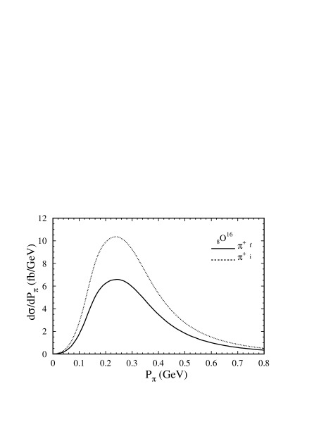
Figure 4: The same as in Fig. 3 for $\pi^{+}$’s on Oxygen target.

Figures 3 and 4 show the same results for charged–current neutrino–production where the $\pi^{+}$ is largely reduced and the $\pi^{0}$ yield slightly increased. In Table 2 we present the transport function $f(\lambda=1)$ for several nuclei where the effect of the absorption cross section is now evident.

${}_{z}T^{A}$	$f(\lambda=1)$
${}_{6}{\rm C}^{12}$	0.81
${}_{8}{\rm O}^{16}$	0.80
${}_{18}{\rm A}^{40}$	0.65
${}_{26}{\rm Fe}^{56}$	0.63

Table 2: The transport function $f(\lambda=1)$.

In addition, we computed the charge–exchange matrix for several values of the absorption cross section and found that it affects $A$ by noticeable amounts but the $3\times 3$ charge–exchange matrix very little ( 3%). Values for the charge–exchange matrix were reported already and we give values for several nuclei.

Carbon

$$A=0.79\,,\quad M(_{6}{\rm C}^{12})=A\left(\begin{array}[]{ccc}0.83&0.14&0.04\\ 0.14&0.73&0.14\\ 0.04&0.14&0.83\end{array}\right)$$

Oxygen

$$A=0.78\,,\quad M(_{8}{\rm O}^{16})=A\left(\begin{array}[]{ccc}0.78&0.16&0.06\\ 0.16&0.68&0.16\\ 0.06&0.16&0.78\end{array}\right)$$

Argon

$$A=0.66\,,\quad M(_{18}{\rm Ar}^{40})=A\left(\begin{array}[]{ccc}0.73&0.19&0.08\\ 0.19&0.63&0.18\\ 0.08&0.18&0.73\end{array}\right)$$

These matrices have been used for analyzing ratios of neutral to charged currents [5]. We mention two examples in order to show the changes that are introduced by rescatterings on nuclei.

Example 1

This case considers the ratio of neutral to charged–current reactions

$$R^{\prime}(_{z}T^{A})=\frac{\sigma(\nu_{\mu}+T\to\nu_{\mu}+\pi^{0})}{2\sigma(\nu_{\mu}+T\to\mu^{-}+\pi^{0})}$$ (46)

which has been measured in two neutrino experiments [6, 7]. The Columbia–BNL experiment had a complex target consisting 75% Al and 25% C. They reported the value [6]

$$R^{\prime}(_{13}{\rm Al}^{37})=0.17\pm 0.06\,.$$ (47)

The Gargamelle experiment used a bubble chamber filled with Freon CF₃Br and reported [7]

$$0.11<R^{\prime}({\rm Br})<0.22\,.$$ (48)

The two experiments are consistent with each other. The values are, however, much smaller than the value calculated for the scattering on free protons and neutrons to be denoted by

$$R(N_{T})=0.44\quad{\rm for}\quad\sin^{2}\theta_{W}=0.22\,.$$ (49)

The agreement is restored [8] when charge–exchange corrections are included

$$R_{\rm theory}(_{13}{\rm Al}^{37})=0.22\,.$$ (50)

This example shows the important role that nuclear corrections played in establishing the isospin content of the neutral current. The same ratio could be, hopefully, measured in K2K, Superkamiokande (SK) and Miniboone. For the long–base–line experiment K2K there is an additional bonus: the ratios should be larger in SK because as the $\nu_{\mu}$’s travel to Kamioka they oscillate to $\nu_{\tau}$’s which do not contribute to the charged–current cross section in the denominator. The precise value of the ratio for the two detectors is calculable.

Example 2

Another realistic case occurred in the Gargamelle experiment where they measured the production of pions in an enriched Freon target. The average energy of the neutrino beam was low, in the $\Delta$–resonance region. They observed the ratio [7]:

$$\frac{\pi^{+}}{\pi^{0}}=2.3\pm 0.9\,.$$ (51)

The cross sections for $E_{\nu}=2.0$ GeV in units of $10^{-38}{\rm cm}^{2}$ are

$$\sigma(\nu p\to\mu^{-}p\pi^{+}) = 0.70\pm 0.10,$$ (52)

$$\sigma(\nu n\to\mu^{-}p\pi^{0}) = 0.20\pm 0.05,$$ (53)

$$\sigma(\nu n\to\mu^{-}n\pi^{+}) = 0.20\pm 0.07\,.$$ (54)

It follows from these numbers that the ratio, averaged over protons and neutrons, is

$$\left(\frac{\pi^{+}}{\pi^{0}}\right)_{{\rm free}\,\frac{(p+n)}{2}}=4.50\,,$$ (55)

which is far away from the value reported by Gargamelle. After we include nuclear corrections for Bromine, the ratio becomes

$$\left(\frac{\pi^{+}}{\pi^{0}}\right)_{\rm nuclear\,\,corrected}=2.64$$ (56)

in good agreement with the experimental number.

Further information on the pion absorption cross section could be extracted [9] from an Argonne experiment on Deuterium [10] and data from the BEBC experiment [11] on a Neon target. Deuterium was considered to be an isoscalar target of free protons and neutrons, and nuclear corrections were introduced for Neon. Unfortunately, the two experiments were at different energies. However, it was possible to re-weight the data to the same atmospheric neutrino energy spectrum [12] allowing for a direct comparison. The parameters of the ANP model were found to be in good qualitative agreement with the data [9].

The comparisons show that the qualitative properties of the pion transport model are confirmed by experiments. The remaining question is to test the degree of its accuracy. This can and should be done in the running and upcoming experiments because the model provides a means for studying the mixing and other properties of neutrinos to a higher degree of accuracy. Precise determinations of nuclear corrections are also important for the discovery of CP–violation in the leptonic sector.

Acknowlegdement

We wish to thank Dr. M. Sakuda for several useful discussions and the organizers for a productive and pleasant meeting at Gran Sasso.

References

- [1] Y. Obayashi, Nucl. Phys. (Proc. Suppl.) 112, 18 (2002).
- [2] S.L. Adler, S. Nussinov, and E.A. Paschos, Phys. Rev. D9, 2125 (1974).
- [3] Landölt–Börnstein, Numerical Data and Functional Relationships: Nuclear Radii, Springer-Verlag (1967).
- [4] For earlier work on the angular dependence of pions see: D. Rein, Z. Phys. C35, 43 (1987), M. Nowakowski, Z. Phys. C35, 129 (1987). This type of work must be updated for several of the resonances.
- [5] S.L. Adler, Phys. Rev. D12, 2644 (1975).
- [6] W. Lee et al., Phys. Rev. Lett. 38, 202 (1977).
- [7] P. Musset and J.P. Vialle, Phys. Rept. 39, 1 (1978), p. 101.
- [8] See Tables II and III on pages 2134 and 2135 of ref. [2].
- [9] For some parametrizations see: I. Schienbein and J.-Y. Yu, Proceedings of the 2nd Int. Workshop on Neutrino–Nucleon Interaction (NUINT ’02), hep-ph/0308010.
-
[10]
S.J. Barish, Phys. Rev. D16, 3103 (1977),
G. Radecky et al., ibid. 25, 1161 (1982). - [11] C. Angelini et al., Phys. Lett. B179, 307 (1986).
- [12] R. Merenyi et al., Phys. Rev. D45, 743 (1992).