UWThPh-2004-19
	OCHA-PP-244
	January 19, 2005

Non-vanishing $U_{e3}$ and $\cos{2\theta_{23}}$ from a broken $Z_{2}$ symmetry

Walter Grimus,^a  Anjan S. Joshipura,^b  Satoru Kaneko,^c

Luís Lavoura,^d  Hideyuki Sawanaka ^e  and Morimitsu Tanimoto$\,{}^{f}$

${}^{a}\!$ Institut für Theoretische Physik, Universität Wien, Boltzmanngasse 5, A–1090 Wien, Austria

${}^{b}\!$ Physical Research Laboratory, Ahmedabad 380009, India

${}^{c}\!$ Department of Physics, Ochanomizu University, Tokyo 112-8610, Japan

${}^{d}\!$ Instituto Superior Técnico, Universidade Técnica de Lisboa, P–1049-001 Lisboa, Portugal

${}^{e}\!$ Graduate School of Science and Technology, Niigata University, 950-2181 Niigata, Japan

${}^{f}\!$ Department of Physics, Niigata University, 950-2181 Niigata, Japan

ABSTRACT

It is shown that the neutrino mass matrices in the flavour basis yielding a vanishing $U_{e3}$ are characterized by invariance under a class of $Z_{2}$ symmetries. A specific $Z_{2}$ in this class also leads to a maximal atmospheric mixing angle $\theta_{23}$. The breaking of that $Z_{2}$ can be parameterized by two dimensionless quantities, $\epsilon$ and $\epsilon^{\prime}$; the effects of $\epsilon,\epsilon^{\prime}\neq 0$ are studied perturbatively and numerically. The induced value of $\left|U_{e3}\right|$ strongly depends on the neutrino mass hierarchy. We find that $\left|U_{e3}\right|$ is less than $0.07$ for a normal mass hierarchy, even when $\epsilon,\epsilon^{\prime}\sim 30\%$. For an inverted mass hierarchy $\left|U_{e3}\right|$ tends to be around $0.1$ but can be as large as $0.17$. In the case of quasi-degenerate neutrinos, $\left|U_{e3}\right|$ could be close to its experimental upper bound $0.2$. In contrast, $\left|\cos{2\theta_{23}}\right|$ can always reach its experimental upper bound $0.28$. We propose a specific model, based on electroweak radiative corrections in the MSSM, for $\epsilon$ and $\epsilon^{\prime}$. In that model, both $\left|U_{e3}\right|$ and $\left|\cos{2\theta_{23}}\right|$, could be close to their respective experimental upper bounds if neutrinos are quasi-degenerate.

1 Introduction

In recent years, the observation of solar [1, 2] and atmospheric [3] neutrino oscillations has dramatically improved our knowledge of neutrino masses and lepton mixing. The neutrino mass-squared differences $\Delta_{\rm sun}$ and $\Delta_{\rm atm}$, and the mixing angles $\tan^{2}{\theta_{\rm sun}}$ and $\sin^{2}{2\theta_{\rm atm}}$, are now quite well determined. The third mixing angle, represented by the matrix element $U_{e3}$ of the lepton mixing matrix $U$ (MNS matrix [4]), is constrained to be small by the non-observation of neutrino oscillations at the CHOOZ experiment [5].

In spite of all this progress, the available information on neutrino masses and lepton mixing is not sufficient to uncover the mechanism of neutrino mass generation. In particular, we do not yet know whether the observed features of lepton mixing are due to some underlying flavour symmetry, or they are mere mathematical coincidences [6] of the seesaw mechanism. Two features of lepton mixing which would suggest a definite symmetry are the small magnitudes of $U_{e3}$ and $\cos{2\theta_{23}}$, where $\theta_{23}$ is one of the angles in the standard parameterization of the MNS matrix and coincides with the atmospheric mixing angle $\theta_{\rm atm}$ when $U_{e3}=0.$ The best-fit value for $\theta_{23}$ in a two-generation analysis [3] of the atmospheric data is $\theta_{23}=\pi/4$, corresponding to $\cos{2\theta_{23}}=0$. Likewise, $\left|U_{e3}\right|$ is required to be small: $\left|U_{e3}\right|\leq 0.26$ at $3\sigma$ from a combined analysis of the atmospheric and CHOOZ data [7]. This smallness strongly hints at some flavour symmetry.

There are many examples of symmetries which can force $U_{e3}$ and/or $\cos{2\theta_{23}}$ to vanish. Both quantities vanish in the extensively studied bi-maximal mixing Ansatz [8, 9, 10, 11], which can be realized through a symmetry [12]. One can also make both $U_{e3}$ and $\cos{2\theta_{23}}$ zero while leaving the solar mixing angle arbitrary [13, 14]. Alternatively, it is possible to force only $U_{e3}$ to be zero, by imposing a discrete Abelian [15] or non-Abelian [16] symmetry; conversely, one can obtain maximal atmospheric mixing but a free $U_{e3}$ by means of a non-Abelian symmetry or a non-standard CP symmetry [17].

The symmetries mentioned above need not be exact. It is important to consider perturbations of those symmetries from the phenomenological point of view and to study quantitatively [18] the magnitudes of $U_{e3}$ and $\cos{2\theta_{23}}$ possibly generated by such perturbations.

This paper is a study of a special class of symmetries and of the consequences of their perturbative violation. We show in section 2 that $U_{e3}$ vanishes if the neutrino mass matrix in the flavour basis is invariant under a class of $Z_{2}$ symmetries. The solar and atmospheric mixing angles, as well as the neutrino masses, remain unconstrained by these $Z_{2}$ symmetries. Those $Z_{2}$ symmetries thus constitute a general class of symmetries leading only to a vanishing $U_{e3}$. We point out that there is a special $Z_{2}$ in this class which leads, furthermore, to maximal atmospheric mixing. We consider more closely that specific $Z_{2}$ in section 3, wherein we study departures from the symmetric limit. We parameterize perturbations of the $Z_{2}$-invariant mass matrix in terms of two complex parameters, and derive general expressions for $U_{e3}$ and $\cos{2\theta_{23}}$ in terms of those parameters; we also present detailed numerical estimates of $U_{e3}$ and $\cos{2\theta_{23}}$. Section 4 is devoted to the study of the specific perturbation which is induced by the electroweak radiative corrections to a $Z_{2}$-invariant neutrino mass matrix defined at a high scale. We discuss a specific model for this scenario. In the concluding section 5 we make a comparison of the predictions for $\left|U_{e3}\right|$ and $\cos{2\theta_{23}}$ obtained within various frameworks.

2 Vanishing $U_{e3}$ from a class of $Z_{2}$ symmetries

The neutrino masses and lepton mixing are completely determined by the neutrino mass matrix in the flavour basis—the basis where the charged-lepton mass matrix is diagonal—which we denote as ${\mathcal{M}}_{\nu f}$. In this section we look for effective symmetries of ${\mathcal{M}}_{\nu f}$ which may lead to a vanishing $U_{e3}$.

One knows [19] that the lepton-number symmetry $L_{e}-L_{\mu}-L_{\tau}$ implies ($i$) a vanishing solar mass-squared difference $\Delta_{\rm sun}$, ($ii$) a maximal solar mixing angle $\theta_{23}$, and ($iii$) a vanishing $U_{e3}$, while it keeps the atmospheric mixing angle unconstrained; one must introduce [20] a significant breaking of $L_{e}-L_{\mu}-L_{\tau}$ in order to correct the predictions ($i$) and ($ii$). A better symmetry seems to be the $\mu$–$\tau$ interchange symmetry [13], which implies vanishing $U_{e3}$ and maximal $\theta_{23}$, but leaves both the neutrino masses and the solar mixing angle unconstrained; this is consistent with the present experimental results. The $\mu$–$\tau$ interchange symmetry can be physically realized in a model based on the discrete non-Abelian group $D_{4}$ [14]; a variation of this model [16] keeps the prediction $U_{e3}=0$ but leaves the atmospheric mixing angle arbitrary. Recently, Low [15] has considered models wherein ${\mathcal{M}}_{\nu f}$ has, due to a discrete Abelian symmetry, a structure leading to $U_{e3}=0$.

We now show that there exists a class $Z_{2}\left(\gamma,\alpha\right)$ of discrete symmetries of the $Z_{2}$ type which encompasses all the models discussed above and enforces a form of ${\mathcal{M}}_{\nu f}$ leading to $U_{e3}=0$. This class is parametrized by an angle $\gamma$ ($0<\gamma<2\pi$) and a phase $\alpha$ ($0\leq\alpha<2\pi$). The symmetry $Z_{2}\left(\gamma,\alpha\right)$ is defined by the $3\times 3$ matrix

$$S\left(\gamma,\alpha\right)=\left(\matrix{1&0&0\cr 0&\cos{\gamma}&e^{-i\alpha}\sin{\gamma}\cr 0&e^{i\alpha}\sin{\gamma}&-\cos{\gamma}\cr}\right).$$ (1)

This matrix is unitary; indeed, it satisfies

$$\left[S\left(\gamma,\alpha\right)\right]^{2} = 1_{3\times 3},$$ (2)

$$\left[S\left(\gamma,\alpha\right)\right]^{T} = \left[S\left(\gamma,\alpha\right)\right]^{\ast}.$$ (3)

Equation (2) means that $S\left(\gamma,\alpha\right)$ is a realization of the group $Z_{2}$. We define the $Z_{2}\left(\gamma,\alpha\right)$ invariance of ${\mathcal{M}}_{\nu f}$ by

$$\left[S\left(\gamma,\alpha\right)\right]^{T}{\mathcal{M}}_{\nu f}S\left(\gamma,\alpha\right)={\mathcal{M}}_{\nu f}.$$ (4)

If one writes

$${\mathcal{M}}_{\nu f}=\left(\matrix{\tilde{X}&\tilde{A}&\tilde{B}\cr\tilde{A}&\tilde{C}&\tilde{D}\cr\tilde{B}&\tilde{D}&\tilde{E}\cr}\right),$$ (5)

where all the matrix elements are complex in general, then equation (4) is equivalent to

$$\begin{array}[]{rcl}{\displaystyle\frac{\tilde{B}}{\tilde{A}}-e^{-i\alpha}\tan{\frac{\gamma}{2}}}&=&0,\\[5.69054pt] \left(e^{i\alpha}\tilde{E}-e^{-i\alpha}\tilde{C}\right)\sin{\gamma}+2\tilde{D}\cos{\gamma}&=&0.\end{array}$$ (6)

Let us first prove that the $Z_{2}\left(\gamma,\alpha\right)$ invariance of ${\mathcal{M}}_{\nu f}$ implies $U_{e3}=0$. The matrix $S\left(\gamma,\alpha\right)$ has a unique eigenvalue $-1$ corresponding to the eigenvector

$$v=\left(\begin{array}[]{c}0\\[2.84526pt] {\displaystyle\exp\left(-i\alpha/2\right)\sin{\left(\gamma/2\right)}}\\[5.69054pt] {-\displaystyle\exp\left(i\alpha/2\right)\cos{\left(\gamma/2\right)}}\end{array}\right).$$ (7)

Equation (4), together with $S\left(\gamma,\alpha\right)v=-v$, imply that $\left[S\left(\gamma,\alpha\right)\right]^{T}\left({\mathcal{M}}_{\nu f}\,v\right)=-\left({\mathcal{M}}_{\nu f}\,v\right)$. Then, equation (3), together with the fact that the eigenvalue $-1$ of $S\left(\gamma,\alpha\right)$ is unique, implies that ${\mathcal{M}}_{\nu f}\,v\propto v^{\ast}$. Now, ${\mathcal{M}}_{\nu f}$ determines the lepton mixing matrix—MNS matrix—$U$ according to

$${\mathcal{M}}_{\nu f}=U^{\ast}{\rm diag}\left(m_{1},m_{2},m_{3}\right)U^{\dagger},$$ (8)

where $m_{1}$, $m_{2}$, and $m_{3}$ are the (real and non-negative) neutrino masses. Thus, if we write $U=\left(u_{1},u_{2},u_{3}\right)$, then the column vectors $u_{j}$ satisfy ${\mathcal{M}}_{\nu f}u_{j}=m_{j}u_{j}^{\ast}$ for $j=1,2,3$. The fact that ${\mathcal{M}}_{\nu f}\,v\propto v^{\ast}$ therefore means that, apart from a phase factor, $v$ is one of the columns of the MNS matrix, hence $U_{e3}=0$, q.e.d.

Let us next prove the converse of the above, i.e. that $U_{e3}=0$ implies that there is some angle $\gamma$ and phase $\alpha$ such that ${\mathcal{M}}_{\nu f}$ is $Z_{2}\left(\gamma,\alpha\right)$-invariant. If $U_{e3}=0$ then $U$ may be parametrized by two angles $\vartheta_{1,2}$ and five phases $\chi_{1,2,3,4,5}$ as

$$U=\left(\begin{array}[]{ccc}e^{i\chi_{1}}\cos{\vartheta_{1}}&e^{i\chi_{2}}\sin{\vartheta_{1}}&0\\ -e^{i\chi_{3}}\sin{\vartheta_{1}}\cos{\vartheta_{2}}&e^{i\left(\chi_{2}+\chi_{3}-\chi_{1}\right)}\cos{\vartheta_{1}}\cos{\vartheta_{2}}&e^{i\chi_{4}}\sin{\vartheta_{2}}\\ e^{i\chi_{5}}\sin{\vartheta_{1}}\sin{\vartheta_{2}}&-e^{i\left(\chi_{2}+\chi_{5}-\chi_{1}\right)}\cos{\vartheta_{1}}\sin{\vartheta_{2}}&e^{i\left(\chi_{4}+\chi_{5}-\chi_{3}\right)}\cos{\vartheta_{2}}\end{array}\right).$$ (9)

When one computes ${\mathcal{M}}_{\nu f}$ through equation (8) one then finds that it satisfies equations (6) with $\gamma/2=\vartheta_{2}$ and $\alpha=\chi_{5}-\chi_{3}+\pi$, q.e.d.

One has thus proved the equivalence of $U_{e3}=0$ with the existence of some angle $\gamma$ and phase $\alpha$ such that ${\mathcal{M}}_{\nu f}$ is $Z_{2}\left(\gamma,\alpha\right)$-invariant.

It should be stressed that $Z_{2}\left(\gamma,\alpha\right)$ will not usually be a symmetry of the full model, nor is it necessarily the remaining symmetry of some larger symmetry operating at a high scale. Some examples may help making this clear:

• The $\mu$–$\tau$ interchange symmetry [13], which corresponds to $\cos{\gamma}=0,\ e^{i\alpha}\sin{\gamma}=1$, cannot be a symmetry of the full theory, since the masses of the $\mu$ and $\tau$ charged leptons are certainly different; thus, that symmetry must be broken in the charged-lepton mass matrix, but that breaking must occur in such a way that it remains unseen—at least at tree level—in the form of ${\mathcal{M}}_{\nu f}$. Moreover, the $\mu$–$\tau$ interchange symmetry predicts $\cos{2\theta_{23}}=0$ together with $U_{e3}=0$.

• Many models based on $\overline{L}=L_{e}-L_{\mu}-L_{\tau}$ lead to [19]

  $${\mathcal{M}}_{\nu f}=\left(\begin{array}[]{ccc}x&y&ry\\ y&z&rz\\ ry&rz&r^{2}z\end{array}\right).$$ (10)

  In this case $\cos{\gamma}=\left(1-|r|^{2}\right)/\left(1+|r|^{2}\right)$ and $e^{i\alpha}\sin{\gamma}=2r^{\ast}/\left(1+|r|^{2}\right)$. The symmetry $Z_{2}\left(\gamma,\alpha\right)$ is not a subgroup of the original $\overline{L}$ symmetry, rather it occurs accidentally as a consequence of the specific particle content of the models and of the particular way in which $\overline{L}$ is softly broken. The mass matrix in equation (10) predicts $m_{3}=0$ together with $U_{e3}=0$.

• The softly-broken $D_{4}$ model [16] has

  $${\mathcal{M}}_{\nu f}^{-1}=\left(\begin{array}[]{ccc}x&y&t\\ y&z&0\\ t&0&z\end{array}\right),$$ (11)

  together with the condition $\arg{y^{2}}=\arg{t^{2}}$. In this case $\cos{\gamma}=\left(y^{2}-t^{2}\right)/\left(y^{2}+t^{2}\right)$ and $e^{i\alpha}\sin{\gamma}=2yt/\left(y^{2}+t^{2}\right)$. The fact that the $\left(\mu,\tau\right)$ matrix element of ${\mathcal{M}}_{\nu f}^{-1}$ is zero, and the fact that its $\left(\mu,\mu\right)$ and $\left(\tau,\tau\right)$ matrix elements remain equal, are just reflections of the limited particle content used to break the original $D_{4}$ symmetry softly.

Thus, the symmetry $Z_{2}\left(\gamma,\alpha\right)$ may be fundamental, effective, or accidental, depending on the specific model at hand.

Considering equation (9) more carefully one notices that the phase $\alpha=\chi_{5}-\chi_{3}+\pi$ is physically meaningless, since it can be removed through a rephasing of the charged-lepton fields. Let us then set $\alpha=0$. In that case, the ${\mathcal{M}}_{\nu f}$ satisfying equations (6) can be written in the form

$${\mathcal{M}}_{\nu f}=\left(\matrix{X&\sqrt{2}A\cos{\left(\gamma/2\right)}&\sqrt{2}A\sin{\left(\gamma/2\right)}\cr\sqrt{2}A\cos{\left(\gamma/2\right)}&B+C\cos{\gamma}&C\sin{\gamma}\cr\sqrt{2}A\sin{\left(\gamma/2\right)}&C\sin{\gamma}&B-C\cos{\gamma}\cr}\right).$$ (12)

The eigenvalue corresponding to the eigenvector in equation (7) is $B-C$.

Specific choices of the parameters in equation (12) give different models. The model with $B=C=X=0$ corresponds to $L_{e}-L_{\mu}-L_{\tau}$ symmetry [19]. The model with $\gamma=\pi/2$ corresponds to $\mu$–$\tau$ interchange symmetry [13]. The $D_{4}$ model in [16] has $\tilde{X}=\tilde{A}^{2}/\tilde{D}$. Likewise, various models in [15] can be shown to have a ${\mathcal{M}}_{\nu f}$ which is formally identical to the matrix in equation (12).

In this paper we modify the standard parametrization for $U$ by multiplying its third row by $-1$, i.e. we use

$$U=\left(\matrix{c_{13}c_{12}&c_{13}s_{12}&s_{13}e^{-i\delta}\cr-c_{23}s_{12}-s_{23}s_{13}c_{12}e^{i\delta}&c_{23}c_{12}-s_{23}s_{13}s_{12}e^{i\delta}&s_{23}c_{13}\cr-s_{23}s_{12}+c_{23}s_{13}c_{12}e^{i\delta}&s_{23}c_{12}+c_{23}s_{13}s_{12}e^{i\delta}&-c_{23}c_{13}\cr}\right)\times{\rm diag}\left(e^{i\rho},\ e^{i\sigma},\ 1\right).$$ (13)

Then, if we let $U_{e3}=s_{13}e^{-i\delta}=0$, equation (8) reduces to equation (12) with $\gamma/2=\theta_{23}$ and

$$\begin{array}[]{rcl}X&=&c_{12}^{2}m_{1}e^{-2i\rho}+s_{12}^{2}m_{2}e^{-2i\sigma},\\[5.69054pt] A&=&-{\displaystyle\frac{c_{12}s_{12}}{\sqrt{2}}}\left(m_{1}e^{-2i\rho}-m_{2}e^{-2i\sigma}\right),\\[8.53581pt] B&=&{\displaystyle\frac{1}{2}}\left(s_{12}^{2}m_{1}e^{-2i\rho}+c_{12}^{2}m_{2}e^{-2i\sigma}+m_{3}\right),\\[8.53581pt] C&=&{\displaystyle\frac{1}{2}}\left(s_{12}^{2}m_{1}e^{-2i\rho}+c_{12}^{2}m_{2}e^{-2i\sigma}-m_{3}\right).\end{array}$$ (14)

3 Non-zero $U_{e3}$, $\cos 2\theta_{23}$ from $Z_{2}$ breaking

Models with $U_{e3}=0$ can be divided in two different categories:

• Those in which the solar scale also vanishes, along with $U_{e3}$. These are obtained by setting $m_{1}=m_{2}$ in equations (14). In these models, the perturbation which generates the solar scale can be expected to also generate $U_{e3}$, and one may find [18, 21] correlations between them.

• Models in which the solar scale is present already at the zeroth order. These are represented by equation (12) without additional restrictions on its parameters, except possibly $\gamma=\pi/4$.

We consider here the more general second category, but fix $\gamma=\pi/4$, i.e. we consider models with vanishing $U_{e3}$ and $\cos{2\theta_{23}}$. ${\mathcal{M}}_{\nu f}$ can be explicitly written in this case as

$${\mathcal{M}}_{\nu f}=U_{0}^{\ast}{\rm diag}\left(m_{1},m_{2},m_{3}\right)U_{0}^{\dagger},$$ (15)

where $U_{0}$ is obtained from equation (13) by setting $s_{13}=0$ and $\theta_{23}=\pi/4$. One then has

$${\mathcal{M}}_{\nu f}=\left(\matrix{X&A&A\cr A&B&C\cr A&C&B\cr}\right).$$ (16)

Consider a general perturbation $\delta{\mathcal{M}}_{\nu f}$ to equation (16). The matrix $\delta{\mathcal{M}}_{\nu f}$ is a general complex symmetric matrix, but part of it can be absorbed through a redefinition of the parameters in equation (16). The remaining part can be written, without loss of generality, as

$$\delta{\mathcal{M}}_{\nu f}=\left(\matrix{0&\epsilon_{1}&-\epsilon_{1}\cr\epsilon_{1}&\epsilon_{2}&0\cr-\epsilon_{1}&0&-\epsilon_{2}\cr}\right).$$ (17)

The perturbation is controlled by two parameters, $\epsilon_{1}$ and $\epsilon_{2}$, which are complex and model-dependent. We want to study their effects perturbatively, i.e. we want to assume $\epsilon_{1}$ and $\epsilon_{2}$ to be small. This smallness can be quantified by saying either that they are smaller than the largest element in ${\mathcal{M}}_{\nu f}$, or that the perturbation to a given matrix element of ${\mathcal{M}}_{\nu f}$ is smaller than the element itself. We adopt the latter alternative and define two dimensionless parameters:

$$\epsilon_{1}\equiv\epsilon A,\quad\epsilon_{2}\equiv\epsilon^{\prime}B.$$ (18)

Thus, we have the neutrino mass matrix with $Z_{2}$ breaking as follows:

$${\mathcal{M}}_{\nu f}=\left(\matrix{X&A\left(1+\epsilon\right)&A\left(1-\epsilon\right)\cr A\left(1+\epsilon\right)&B\left(1+\epsilon^{\prime}\right)&C\cr A\left(1-\epsilon\right)&C&B\left(1-\epsilon^{\prime}\right)\cr}\right)\ ,$$ (19)

where we shall assume $\epsilon$ and $\epsilon^{\prime}$ to be small, $\left|\epsilon\right|,\left|\epsilon^{\prime}\right|\ll 1$.

One finds that, to first order in $\epsilon$ and $\epsilon^{\prime}$, the only effect of the $\delta{\mathcal{M}}_{\nu f}$ in equation (17) is to generate non-zero $U_{e3}$ and $\cos{2\theta_{23}}$. The neutrino masses, as well as the solar angle, do not receive any corrections. $U_{e3}$ and $\cos{2\theta_{23}}$ are of the same order as $\epsilon$ and $\epsilon^{\prime}$. Define

$$\hat{m}_{1} \equiv m_{1}e^{-2i\rho},$$ (20)

$$\hat{m}_{2} \equiv m_{2}e^{-2i\sigma},$$ (21)

and

$$\overline{\epsilon} \equiv \left(\hat{m}_{1}-\hat{m}_{2}\right)\epsilon,$$ (22)

$$\overline{\epsilon}^{\prime} \equiv \frac{\hat{m}_{1}s_{12}^{2}+\hat{m}_{2}c_{12}^{2}+m_{3}}{2}\,\epsilon^{\prime}.$$ (23)

Then, we get

$$U_{e3} = \frac{s_{12}c_{12}}{m_{3}^{2}-m_{2}^{2}}\left(\overline{\epsilon}s_{12}^{2}\hat{m}_{2}^{\ast}+\overline{\epsilon}^{\ast}s_{12}^{2}m_{3}-\overline{\epsilon}^{\prime}\hat{m}_{2}^{\ast}-{\overline{\epsilon}^{\prime}}^{\ast}m_{3}\right)$$ (24)

$$+\frac{s_{12}c_{12}}{m_{3}^{2}-m_{1}^{2}}\left(\overline{\epsilon}c_{12}^{2}\hat{m}_{1}^{\ast}+\overline{\epsilon}^{\ast}c_{12}^{2}m_{3}+\overline{\epsilon}^{\prime}\hat{m}_{1}^{\ast}+{\overline{\epsilon}^{\prime}}^{\ast}m_{3}\right),$$

$$\cos{2\theta_{23}} = {\rm Re}\left\{\frac{2c_{12}^{2}}{m_{3}^{2}-m_{2}^{2}}\left(\overline{\epsilon}s_{12}^{2}-\overline{\epsilon}^{\prime}\right)\left(\hat{m}_{2}+m_{3}\right)^{\ast}-\frac{2s_{12}^{2}}{m_{3}^{2}-m_{1}^{2}}\left(\overline{\epsilon}c_{12}^{2}+\overline{\epsilon}^{\prime}\right)\left(\hat{m}_{1}+m_{3}\right)^{\ast}\right\}.$$ (25)

The meaningful phases in ${\mathcal{M}}_{\nu f}$ are the ones of rephasing-invariant quartets. Since ${\mathcal{M}}_{\nu f}$ is symmetric, there are three such phases which are linearly independent. (Correspondingly, there are three physical phases in the MNS matrix: $\delta$, $2\rho$, and $2\sigma$.) One easily sees that, in the first-order approximation in $\epsilon$ and $\epsilon^{\prime}$, the imaginary parts of those two small parameters are meaningless when taken separately; only $\mathrm{Im}\left(2\epsilon-\epsilon^{\prime}\right)$ is physically meaningful to this order. Indeed, one can manipulate equations (24) and (25) to obtain

$$\cos{2\theta_{23}} = \left\{\frac{c_{12}^{2}}{m_{2}^{2}-m_{3}^{2}}\left[m_{3}^{2}+c_{12}^{2}m_{2}^{2}+s_{12}^{2}{\rm Re}\left(\hat{m}_{1}\hat{m}_{2}^{\ast}+\hat{m}_{1}m_{3}\right)+\left(1+c_{12}^{2}\right){\rm Re}\left(\hat{m}_{2}m_{3}\right)\right]\right.$$ (26)

$$\left.+\frac{s_{12}^{2}}{m_{1}^{2}-m_{3}^{2}}\left[m_{3}^{2}+s_{12}^{2}m_{1}^{2}+c_{12}^{2}{\rm Re}\left(\hat{m}_{2}\hat{m}_{1}^{\ast}+\hat{m}_{2}m_{3}\right)+\left(1+s_{12}^{2}\right){\rm Re}\left(\hat{m}_{1}m_{3}\right)\right]\right\}{\rm Re}\,\epsilon^{\prime}$$

$$+2c_{12}^{2}s_{12}^{2}\left[\frac{m_{2}^{2}-{\rm Re}\left(\hat{m}_{1}\hat{m}_{2}^{\ast}+\hat{m}_{1}m_{3}-\hat{m}_{2}m_{3}\right)}{m_{2}^{2}-m_{3}^{2}}\right.$$

$$\left.+\frac{m_{1}^{2}-{\rm Re}\left(\hat{m}_{1}\hat{m}_{2}^{\ast}-\hat{m}_{1}m_{3}+\hat{m}_{2}m_{3}\right)}{m_{1}^{2}-m_{3}^{2}}\right]{\rm Re}\,\epsilon$$

$$+\frac{c_{12}^{2}s_{12}^{2}\left(m_{1}^{2}-m_{2}^{2}\right){\rm Im}\left(\hat{m}_{1}\hat{m}_{2}^{\ast}+\hat{m}_{1}m_{3}+\hat{m}_{2}^{\ast}m_{3}\right)}{\left(m_{3}^{2}-m_{1}^{2}\right)\left(m_{3}^{2}-m_{2}^{2}\right)}\,{\rm Im}\left(2\epsilon-\epsilon^{\prime}\right),$$

$$\frac{U_{e3}}{c_{12}s_{12}} = \frac{1}{2}\left\{\frac{1}{m_{2}^{2}-m_{3}^{2}}\left[s_{12}^{2}\hat{m}_{1}\hat{m}_{2}^{\ast}+s_{12}^{2}\hat{m}_{1}^{\ast}m_{3}+\left(1+c_{12}^{2}\right)\hat{m}_{2}^{\ast}m_{3}+m_{3}^{2}+c_{12}^{2}m_{2}^{2}\right]\right.$$ (27)

$$\left.+\frac{1}{m_{3}^{2}-m_{1}^{2}}\left[c_{12}^{2}\hat{m}_{1}^{\ast}\hat{m}_{2}+c_{12}^{2}\hat{m}_{2}^{\ast}m_{3}+\left(1+s_{12}^{2}\right)\hat{m}_{1}^{\ast}m_{3}+m_{3}^{2}+s_{12}^{2}m_{1}^{2}\right]\right\}{\rm Re}\,\epsilon^{\prime}$$

$$+\left[\frac{s_{12}^{2}}{m_{2}^{2}-m_{3}^{2}}\left(m_{2}^{2}-\hat{m}_{1}\hat{m}_{2}^{\ast}-\hat{m}_{1}^{\ast}m_{3}+\hat{m}_{2}^{\ast}m_{3}\right)\right.$$

$$\left.+\frac{c_{12}^{2}}{m_{3}^{2}-m_{1}^{2}}\left(m_{1}^{2}-\hat{m}_{1}^{\ast}\hat{m}_{2}+\hat{m}_{1}^{\ast}m_{3}-\hat{m}_{2}^{\ast}m_{3}\right)\right]{\rm Re}\,\epsilon$$

$$+\frac{i}{2}\left[\frac{s_{12}^{2}}{m_{2}^{2}-m_{3}^{2}}\left(m_{2}^{2}-\hat{m}_{1}\hat{m}_{2}^{\ast}+\hat{m}_{1}^{\ast}m_{3}-\hat{m}_{2}^{\ast}m_{3}\right)\right.$$

$$\left.+\frac{c_{12}^{2}}{m_{3}^{2}-m_{1}^{2}}\left(m_{1}^{2}-\hat{m}_{1}^{\ast}\hat{m}_{2}-\hat{m}_{1}^{\ast}m_{3}+\hat{m}_{2}^{\ast}m_{3}\right)\right]{\rm Im}\left(2\epsilon-\epsilon^{\prime}\right).$$

The induced values of $\left|U_{e3}\right|$ and $|\cos 2\theta_{23}|$ are strongly correlated to neutrino mass hierarchies. This makes it possible to draw some general conclusions even if we do not know the magnitudes of $\epsilon,\epsilon^{\prime}$. In Table 1 we give expressions and values for $\left|U_{e3}\right|$ and $|\cos 2\theta_{23}|$ in case of the hierarchical ($m_{1}<m_{2}<m_{3}$), inverted ($m_{1}\approx m_{2}\sim\sqrt{\Delta_{\rm atm}}\gg m_{3}$) and quasi-degenerate neutrino spectrum. CP conservation is assumed but we distinguish two different cases (a) the Dirac solar pair corresponding to $\sigma=\rho=0$ and the Pseudo-Dirac solar pair with $\rho=\pi/2,\sigma=0$. We have also given approximate values in some cases assuming the common degenerate mass $m\sim 0.3~{}{\rm eV}$.

It follows from the Table 1 and equations (26,27) that:

• The first order contribution to $U_{e3}$ given in equation (27) vanish identically if $\hat{m}_{1}=\hat{m}_{2}$. As a consequence of this, $U_{e3}$ gets suppressed by a factor ${\mathcal{O}}(\frac{\Delta_{\rm sun}}{\Delta_{\rm atm}})$ for the inverted or quasi-degenerate spectrum with $\rho=\sigma=0$. Similar suppression also occurs in case of the normal neutrino mass hierarchy even when $\rho\not=\sigma$. $U_{e3}$ need not be suppressed in other cases and can be large.

• In contrast to $U_{e3}$, $\cos 2\theta_{23}$ is almost as large as $\epsilon,\epsilon^{\prime}$ if neutrino mass spectrum is normal or inverted. It gets enhanced compared to these parameters if the spectrum is quasi-degenerate.

• In case of the quasi-degenerate spectrum, both $|\cos 2\theta_{23}|$ and $\left|U_{e3}\right|$ can become quite large and reach the present experimental limits. Especially, the enhancement factors are large in case of the pseudo-Dirac solar pair ($\rho=\pi/2$, $\sigma=0$). $U_{e3}$ and $\cos 2\theta_{23}$ are in fact proportional to each other in this particular case. The parameters $\epsilon,\epsilon^{\prime}$ are constrained to be lower than $10^{-2}$ for the quasi-degenerate spectrum.

Normal Hierarchy	$|U_{e3}|\approx c_{12}s_{12}\sqrt{\frac{\Delta_{\rm sun}}{\Delta_{\rm atm}}}(\epsilon+\frac{\epsilon^{\prime}}{2})\approx 0.09(\epsilon+\frac{\epsilon^{\prime}}{2})$
$m_{1}\ll m_{2};m_{2}^{2}\approx\Delta_{\rm sun};m_{3}^{2}\approx\Delta_{\rm atm}$	$|\cos 2\theta_{23}|\approx\epsilon^{\prime}$
Inverted Hierarchy	$|U_{e3}|\approx{\Delta_{\rm sun}\over 2\Delta_{\rm atm}}s_{12}c_{12}(\epsilon-\frac{\epsilon^{\prime}}{2})\approx 0.009(\epsilon-\frac{\epsilon^{\prime}}{2})$
$\sigma=0;\rho=0$	$|\cos 2\theta_{23}|\approx\epsilon^{\prime}$
$\sigma=0;\rho=\pi/2$	$|U_{e3}|\approx\frac{1}{2}\sin 4\theta_{12}(\epsilon-\frac{\epsilon^{\prime}}{2})\approx 0.4(\epsilon-\frac{\epsilon^{\prime}}{2})$
	$|\cos 2\theta_{23}|\approx 2(\epsilon\sin^{2}2\theta_{12}+\frac{\epsilon^{\prime}}{2}\cos^{2}2\theta_{12})$
Quasi-Degenerate	$|U_{e3}|\approx 2\epsilon^{\prime}c_{12}s_{12}{m^{2}\over\Delta_{\rm atm}}\frac{\Delta_{\rm sun}}{\Delta_{\rm atm}}\approx 1.6\epsilon$
$\sigma=0;\rho=0$	$|\cos 2\theta_{23}|\approx 4\frac{m^{2}}{\Delta_{\rm atm}}\epsilon^{\prime}\approx 180\epsilon^{\prime}$
$\sigma=0;\rho=\pi/2$	$|U_{e3}|\approx 4{m^{2}\over\Delta_{\rm atm}}c_{12}s_{12}(\epsilon s_{12}^{2}+\frac{\epsilon^{\prime}}{2}c_{12}^{2})\approx 81(\epsilon s_{12}^{2}+\frac{\epsilon^{\prime}}{2}c_{12}^{2})$
	$|\cos 2\theta_{23}|\approx 8{m^{2}\over\Delta_{\rm atm}}c_{12}^{2}(\epsilon s_{12}^{2}+\frac{\epsilon^{\prime}}{2}c_{12}^{2})\approx 259(\epsilon s_{12}^{2}+\frac{\epsilon^{\prime}}{2}c_{12}^{2})$

Table 1: Leading order predictions for $\left|U_{e3}\right|,\ |\cos 2\theta_{23}|$ in case of different neutrino mass hierarchies with CP conservation. The numerical estimates are based on the best fit values of neutrino parameters and the quasi-degenerate mass $m=0.3{\rm eV}$.

The perturbative expressions given above may not be reliable for some values of $\epsilon,\epsilon^{\prime}$ due to large enhancement factor of ${\mathcal{O}}({m^{2}\over\Delta_{\rm atm}})$ and one should do a numerical analysis. We now discuss results of such analysis in various circumstances. Scattered plots of the predicted values for $|\cos 2\theta_{23}|$ and $\left|U_{e3}\right|$ are given in Figure 1 in the case of normal neutrino mass hierarchy. CP conservation ($\rho=\sigma=0$, real $\epsilon,\epsilon^{\prime}$) is assumed. Neutrino masses and $\theta_{12}$ do not receive any corrections at $O(\epsilon,\epsilon^{\prime})$ and hence do not appreciablly change by perturbations. We therefore randomly varied these input parameters in the experimentally allowed regions. $m_{1}$ was varied up to $m_{2}$. On the other hand, $\epsilon,\epsilon^{\prime}$ are unknown unless the symmetry breaking is specified, so these are varied randomly in the range $-0.3\sim 0.3$ with the condition that the output parameters should lie in the $90\%$ CL limit [2, 7]:

$$0.33\leq\tan^{2}\theta_{\rm sun}\leq 0.49\ ,\ \ 7.7\times 10^{-5}\leq\Delta_{\rm sun}\leq 8.8\times 10^{-5}~{}\rm{eV}^{2},\quad 90\%C.L.\ ,$$

$$0.92\leq\sin^{2}2\theta_{\rm atm}\ ,\ \ 1.5\times 10^{-3}\leq\Delta_{\rm atm}\leq 3.4\times 10^{-3}~{}\rm{eV}^{2},\quad 90\%C.L.\ .$$ (28)

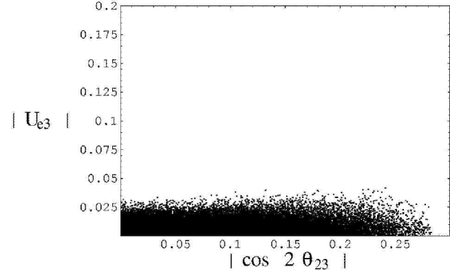
Figure 1: The scattered plots showing the allowed values of $|\cos 2\theta_{23}|$ and $\left|U_{e3}\right|$ in case of the normal neutrino mass hierarchy. $\epsilon,\epsilon^{\prime}$ are randomly varied in the range $-0.3\sim 0.3$. The Majorana phases are chosen as $\rho=0,\ \sigma=0$.

The $\left|U_{e3}\right|$ is forced to be small less than $0.025$, in Figure 1 as would be expected from the foregoing discussion. The value $\sim 0.025$ at the upper end arises from the (assumed) bound $|\epsilon|,|\epsilon^{\prime}|\leq 0.3$. Since $\left|U_{e3}\right|$ is proportional to $\epsilon,\epsilon^{\prime}$, it increases if the bound on $\epsilon,\epsilon^{\prime}$ is loosened. However, $|\epsilon|\leq 0.3$ is a reasonable bound due to assume if $Z_{2}$ breaking is perturbative. On the other hand, $|\cos 2\theta_{23}|$ can assume large values as seen from Figure 1. The present bound $\sin^{2}2\theta_{23}>0.92$ from the atmospheric experiments gets translated to $|\cos 2\theta_{23}|<0.28$ which constrains $|\epsilon^{\prime}|\leq 0.2$ in our analyses.

The non-maximal value for $\theta_{23}$ gives rise to interesting physical effects such as excess of the e-like events in the atmospheric neutrino data in the sub-GeV region [22], different matter dependent survival probabilities for the $\nu_{\mu}$ and the $\overline{\nu}_{\mu}$ [23]. These can be searched for in the future atmospheric [24] and the long baseline experiments. The values $|\cos 2\theta_{23}|>0.1$ are expected to be probed in these experiments [25]. These values occur quite naturally for a reasonably large range of parameters.

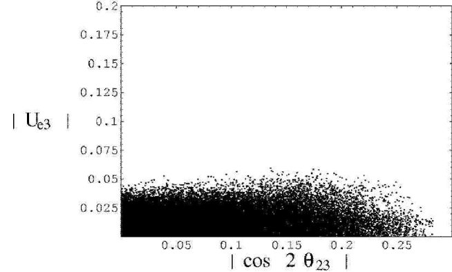
Figure 2: The allowed values $|\cos 2\theta_{23}|$ and $\left|U_{e3}\right|$ for $\rho=\pi/4,\ \sigma=0$ and the normal neutrino mass hierarchy. The other parameters are the same as in Fig. 1.

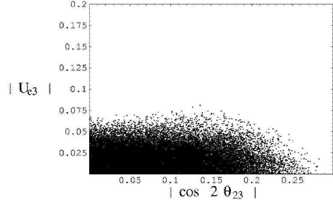
Figure 3: The allowed values $|\cos 2\theta_{23}|$ and $\left|U_{e3}\right|$ for $\rho=\pi/2,\ \sigma=0$ and the normal neutrino mass hierarchy. The other parameters are the same as in Fig. 1.

In order to find the phase dependence of our results, we show the results in the cases of ($\rho=\pi/4,\ \sigma=0$) and ($\rho=\pi/2,\ \sigma=0$). The phase dependence is found in the prediction of $\left|U_{e3}\right|$, which increases up to $0.075$.

The region $\left|U_{e3}\right|>0.07$ is expected to be probed in the long baseline experiments with the conventional or super beams [26] and in the reactor experiments [27]. The smaller values for $\left|U_{e3}\right|\sim 0.025$ can be reached only at the neutrino factory [28]. Most of the region displayed in Figs. 1-3 therefore seem inaccessible to the near future neutrino experiments aimed at searching for $\left|U_{e3}\right|$.

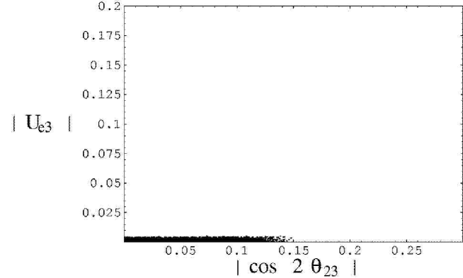
Figure 4: The allowed values of $|\cos 2\theta_{23}|$ and $\left|U_{e3}\right|$ for $\rho=0,\ \sigma=0$ in case of the inverted neutrino mass hierarchy. The $\epsilon,\epsilon^{\prime}$ are varied randomly in the range $-0.3\sim 0.3$ while $m_{3}$ is varied up to $10^{-2}{\rm eV}$.

Scattered plots for the predicted values for $\left|U_{e3}\right|$ and $|\cos 2\theta_{23}|$ are given in Fig. 4 in case of the inverted hierarchy of the neutrino masses. The value of $\left|U_{e3}\right|$ is even more suppressed compared to the corresponding case displayed in Fig. 1. This suppression is due to the strong cancellation between $m_{1}$ and $m_{2}$, which is seen in Table 1. However, the Majorana phases spoil this cancellation, and so $\left|U_{e3}\right|$ could be larger as seen in Figs. 5 and 6, where the two cases ($\rho=\pi/4,\ \sigma=0$) and ($\rho=\pi/2,\ \sigma=0$) are displayed respectively. Thus, the effect of the Majorana phases is very important in the inverted hierarchy. The isolated points in Fig. 6 follows from the tuning of the parameters $\epsilon$ and $\epsilon^{\prime}$. Apart from this tuning, the allowed values of $\left|U_{e3}\right|$ are moderate $\sim 0.1$ but will be explored in the future long baseline and reactor experiments.

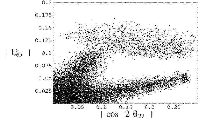
Figure 5: The allowed values of $|\cos 2\theta_{23}|$ and $\left|U_{e3}\right|$ for $\rho=\pi/4,\ \sigma=0$ in case of the inverted neutrino mass hierarchy.

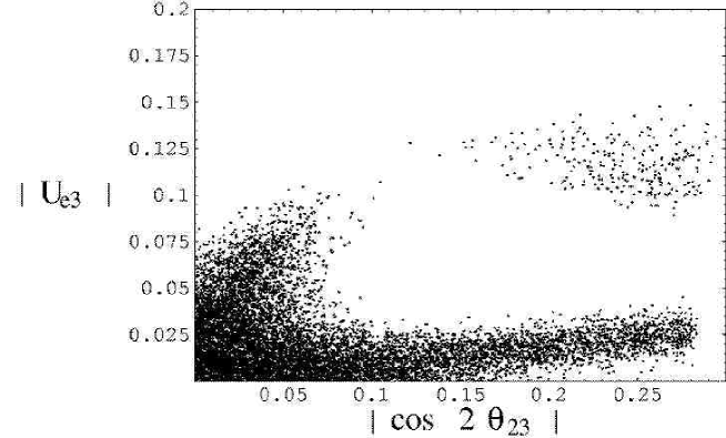
Figure 6: The allowed values of $|\cos 2\theta_{23}|$ and $\left|U_{e3}\right|$ for $\rho=\pi/2,\ \sigma=0$ in case of the inverted neutrino mass hierarchy.

Figure 7: The scattered plots of the allowed values of $|\cos 2\theta_{23}|$ and $\left|U_{e3}\right|$ with $|\epsilon|\leq 0.3$ and $|\epsilon^{\prime}|\leq 0.03$ and the quasi-degenerate neutrino masses. The Majorana phases are chosen as $\rho=0,\ \sigma=0$. The degenerate mass scale is fixed at $m=0.3\ {\rm eV}$.

The parameter $\epsilon^{\prime}$ is constrained strongly $|\epsilon^{\prime}|\leq 0.03$ in case of the quasi-degenerate neutrino masses due to an enhancement factor ${\mathcal{O}}(\frac{m^{2}}{\Delta_{\rm atm}})$ present in this case, as seen in Table 1. $|\epsilon|$ is however not constrained as strongly and we take $|\epsilon|\leq 0.3$. The scattered plots for the predicted values for $\left|U_{e3}\right|$ and $|\cos 2\theta_{23}|$ are given in Fig. 7. The value of $\left|U_{e3}\right|$ is expected to be $O(0.01)$. There are partial cancellations among contributions from $m_{1}$, $m_{2}$, $m_{3}$ when $\rho=\sigma$. However, different choice for the Majorana phases spoil this cancellation and $\left|U_{e3}\right|$ could be large as seen in Figs. 8 and 9, which correspond to ($\rho=\pi/4,\ \sigma=0$) and ($\rho=\pi/2,\ \sigma=0$) respectively. It is found that $\left|U_{e3}\right|$ could increase to $0.1$ in these cases.

Figure 8: The allowed values of $|\cos 2\theta_{23}|$ and $\left|U_{e3}\right|$ in the quasi-degenerate neutrino masses. The Majorana phases are chosen as $\rho=\pi/4,\ \sigma=0$. The degenerate mass scale is fixed at $m=0.3\ {\rm eV}$.

Figure 9: The allowed values of $|\cos 2\theta_{23}|$ and $\left|U_{e3}\right|$ in the quasi-degenerate neutrino masses. The Majorana phases are chosen as $\rho=\pi/2,\ \sigma=0$. The degenerate mass scale is fixed at $m=0.3\ {\rm eV}$.

In the above analyses, we fixed $\sigma=0$ because only the relative phase $\rho-\sigma$ is essential in determining the masses and mixing angles in the case of the hierarchical and inverted hierarchical neutrino masses. However, $\sigma$ dependence is non-trivial for the degenerate masses. We show the results for ($\rho=0,\ \sigma=\pi/2$) and ($\rho=\pi/4,\ \sigma=\pi/2$) in Fig. 10 and Fig. 11 respectively. It is noted that $\left|U_{e3}\right|$ could be as large as $0.2$ for the case $\rho=\pi/4,\ \sigma=\pi/2$ but values $\leq 0.1$ are more probable as seen from the density of points.

Figure 10: The allowed values of $|\cos 2\theta_{23}|$ and $\left|U_{e3}\right|$ in the quasi-degenerate neutrino masses. The Majorana phases are chosen as $\rho=0,\ \sigma=\pi/2$. The degenerate mass scale is fixed at $m=0.3\ {\rm eV}$.

Figure 11: The allowed values of $|\cos 2\theta_{23}|$ and $\left|U_{e3}\right|$ in the quasi-degenerate neutrino masses. The Majorana phases are chosen as $\rho=\pi/4,\ \sigma=\pi/2$. The degenerate mass scale is fixed at $m=0.3\ {\rm eV}$.

Before ending this section, we wish to point out an interesting aspect of this analysis. Since $U_{e3}$ is zero in the absence of the perturbation, the CP violating Dirac phase $\delta$ relevant for neutrino oscillations is undefined at this stage. CP violation is present through the Majorana phases $\rho$ and $\sigma$. Turning on perturbation leads to non-zero $U_{e3}$ and also to a non-zero Dirac phase even if perturbation is real. Moreover, $\delta$ generated this way can be large and independent of the strength of perturbation parameters. This phenomenon was noticed [29] in the specific case of the radiative generation of $U_{e3}$. This occurs here also for a more general perturbation.

As an example, let us consider the limit $\epsilon^{\prime}=0$ and a real $\epsilon$. Since $U_{\mu 3}$ is almost maximal and real, $\delta$ is approximately given by

$$\tan\delta\approx{m_{1}m_{2}\sin 2(\rho-\sigma)-m_{3}m_{1}\sin 2\rho+m_{2}m_{3}\sin 2\sigma+{\mathcal{O}}(\frac{\Delta_{\rm sun}}{\Delta_{\rm atm}})Im({\mathcal{Z}})\over m_{1}^{2}c_{12}^{2}-m_{2}^{2}s_{12}^{2}-m_{1}m_{2}\cos 2\theta_{12}\cos 2(\rho-\sigma)+m_{3}m_{1}\cos 2\rho-m_{2}m_{3}\cos 2\sigma+{\mathcal{O}}(\frac{\Delta_{\rm sun}}{\Delta_{\rm atm}})Re({\mathcal{Z}})}~{},$$ (29)

where ${\mathcal{Z}}\equiv(\hat{m}_{2}^{*}(\hat{m}_{1}-\hat{m_{2}})+m_{3}(\hat{m}_{1}-\hat{m_{2}})^{*})s_{12}^{2}$. It follows from above that irrespective of the specific mass hierarchy, the induced $\delta$ would be large if $\rho$ and $\sigma$ are large and not finetuned.

4 Radiatively generated $U_{e3}$ and $\cos 2\theta_{23}$

The $\epsilon,\epsilon^{\prime}$ were treated as independent parameters so far. They can be related in specific models. We now consider one example which is based on the electroweak breaking of the $Z_{2}$ symmetry in the MSSM. We assume that neutrino masses are generated at some high scale $M_{X}$ and the effective neutrino mass operator describing them is $Z_{2}$ symmetric with the result that $U_{e3}=\cos 2\theta_{23}=0$ at $M_{X}$. This symmetry is assumed to be broken spontaneously in the Yukawa couplings of the charged leptons. This breaking would radiatively induce non-zero $U_{e3}$ and $\cos 2\theta_{23}$ [30]. This can be calculated by using the renormalization group equations (RGEs) of the effective neutrino mass operator [31, 32, 33]. These equations depend upon the detailed structure of the model below $M_{X}$. We assume here that theory below $M_{X}$ is the MSSM and use the RGEs derived in this case. Subsequently we will give an example which realizes our assumptions.

Integration of the RGEs allows us [31, 32, 33] to relate the neutrino mass matrix ${\mathcal{M}}_{\nu f}(M_{X})$ to the corresponding matrix at the low scale which we identify here with the $Z$ mass $M_{Z}$:

$${\mathcal{M}}_{\nu f}(M_{Z})\approx I_{g}I_{t}~{}(I~{}{\mathcal{M}}_{\nu f}(M_{X})~{}I~{})\ ,$$ (30)

where $I_{g,t}$ are calculable numbers depending on the gauge and top quark Yukawa couplings. $I$ is a flavour dependent matrix given by

$$I\approx\mathrm{diag}(1+\delta_{e},1+\delta_{\mu},1+\delta_{\tau})\ ,$$ (31)

with

$$\delta_{\alpha}\approx c\left({m_{\alpha}\over 4\pi v}\right)^{2}\ln{M_{X}\over M_{Z}}~{},$$ (32)

where $c=\frac{3}{2},-\frac{1}{\cos^{2}\beta}$ in case of the Standard Model (SM) and the Minimal Supersymmetric Standard Model (MSSM) respectively [31]. $v$ refers to the vacuum expectation value for the SM Higgs doublet.

We have implicitly neglected possible threshold effects. Inclusion of these effects would not modify the analysis if threshold effects are flavour blind as would be approximately true [34] in case of the minimal supergravity scenario with universal boundary conditions.

${\mathcal{M}}_{\nu f}(M_{X})$ is given by equation (16). From this we can write ${\mathcal{M}}_{\nu f}(M_{Z})$ as follows when the muon and the electron Yukawa couplings are neglected:

$${\mathcal{M}}_{\nu f}(M_{Z}) = \left(\matrix{X&A^{\prime}&A^{\prime}\cr A^{\prime}&B^{\prime}&C^{\prime}\cr A^{\prime}&C^{\prime}&B^{\prime}\cr}\right)+\left(\matrix{0&A^{\prime}\epsilon&-A^{\prime}\epsilon\cr A^{\prime}\epsilon&B^{\prime}\epsilon^{\prime}&0\cr-A^{\prime}\epsilon&0&-B^{\prime}\epsilon^{\prime}\cr}\right)+O(\delta_{\tau}^{2})~{},$$ (33)

where

$$C^{\prime}=C(1+\delta_{\tau})~{}~{},~{}~{}A^{\prime}=A(1+\frac{\delta_{\tau}}{2})~{}~{},~{}~{}B^{\prime}=B(1+\delta_{\tau})~{}~{},~{}~{}\epsilon=\frac{\epsilon^{\prime}}{2}=-\frac{\delta_{\tau}}{2}\ ,$$ (34)

and $A,B,C$ are defined in equation (14). Note that $m_{1}$, $m_{2}$ and $m_{3}$ defined previously are no longer mass eigenvalues because of the changes $A\rightarrow A^{\prime}$, $B\rightarrow B^{\prime}$ and $C\rightarrow C^{\prime}$. Using the above equations, we get from equation (24)

$$U_{e3}\simeq \hskip-14.22636pt-{\delta_{\tau}s_{12}c_{12}\over 2(m_{3}^{2}-m_{1}^{2})}\left[m_{1}^{2}+2m_{3}\hat{m_{1}}^{*}+m_{3}^{2}\right]+{\delta_{\tau}s_{12}c_{12}\over 2m_{3}^{2}-m_{2}^{2}}\left[m_{2}^{2}+2\hat{m_{2}}^{*}m_{3}+m_{3}^{2}\right]\ ,$$

$$\cos 2\theta_{23}\simeq \hskip-14.22636pt{\delta_{\tau}s_{12}^{2}\over m_{3}^{2}-m_{1}^{2}}\left[m_{1}^{2}+2m_{3}\hat{m_{1}}^{*}+m_{3}^{2}\right]+{\delta_{\tau}c_{12}^{2}\over m_{3}^{2}-m_{2}^{2}}\left[m_{2}^{2}+2\hat{m_{2}}^{*}m_{3}+m_{3}^{2}\right]\ .$$ (35)

It is easily seen that the effect of the radiative corrections is enhanced in the case of the quasi-degenerate neutrino masses with opposite phase $|\rho-\sigma|=\pi/2$ as previous works presented [32, 33]. In the MSSM, the parameter $\delta_{\tau}$ is negative and its absolute value can become quite large for large $\tan\beta$, e.g. for $\tan\beta\sim 50,\ |\delta_{\tau}|\sim 0.075$. However, large $\tan\beta$ is not favoured because the renormalization of parameters $A,B,C$ as in equation (34) also shifts the value of the solar angle and solar mass compared to their values in the $\delta_{\tau}\rightarrow 0$ limit. One now gets

$$\Delta_{\rm sun}\cos 2\theta_{\rm sun}\approx\Delta_{21}\cos 2\theta_{12}+2\delta_{\tau}|m_{1}e^{-2i\rho}s_{12}^{2}+m_{2}e^{-2i\sigma}c_{12}^{2}|^{2}~{}.$$ (36)

Here, $\Delta_{21}\equiv m_{2}^{2}-m_{1}^{2}$ and $\theta_{12}$ correspond to the values of the solar scale and angle at $M_{X}$. The radiative corrections add a negative contribution to $\Delta_{\rm sun}\cos 2\theta_{\rm sun}$ in case of the MSSM and can spoil the LMA solution (which need positive $\Delta_{\rm sun}\cos 2\theta_{\rm sun}$) if $\Delta_{21}$ is small or $|\delta_{\tau}|$ is large. This provides a constraint on possible values of $\delta_{\tau}$ and consequently on $|U_{e3}|,|\cos 2\theta_{23}|$ that can be generated in the model. For example, requiring that the first term dominates over the second term in equation (36) implies

$$|\delta_{\tau}|\leq\left({\Delta_{21}\over 2m^{2}\cos 2\theta_{12}}\right)\approx 10^{-3}~{},$$ (37)

where we assumed CP conservation, the quasi-degenerate spectrum, $\sigma=\pi/2;\ \rho=0$ , $m\approx 0.3\ {\rm eV}$, and $\Delta_{21}\sim 8\times 10^{-5}$ eV². The values for $\left|U_{e3}\right|$ and $|\cos 2\theta_{23}|$ implied by the above constraint are quite small. Notice however that one can loosen the bound on $\delta_{\tau}$ by choosing significantly larger value $\Delta_{21}$ than $8\times 10^{-5}{\rm eV}^{2}$. The cancellations between two terms in equation (36) can still lead to physical solar scale.

Figure 12: The scattered plots of the allowed values of $|\cos 2\theta_{23}|$ and $\left|U_{e3}\right|$ in case of the radiatively broken $Z_{2}$ and the quasi-degenerate neutrino masses $m=0.3{\rm eV}$. The Majorana phases are chosen as $\rho=0,\ \sigma=\pi/2$.

Results of the numerical analysis are shown in Fig. 12 in case of the quasi-degenerate spectrum with $m=0.3~{}{\rm eV};\sigma=\pi/2,\rho=0$. The $\theta_{12},\Delta_{21}$ and $\tan\beta$ at high scale are varied randomly, then the allowed choices which reproduce the parameters as in equation (28) at the low scale are determined. Both $\left|U_{e3}\right|$ and $|\cos 2\theta_{23}|$ can reach their respective experimental bound. The near proportionality between the two can be understood from their expressions given in Table 1. We find numerically that $\tan\beta$ is constrained to be lower than $20$ in this case. The forthcoming experiments will be able to test this relationship between $\left|U_{e3}\right|$ and $|\cos 2\theta_{23}|$. It may be useful to note our numerical results of $\left|U_{e3}\right|$ in the cases of the normal-hierarchy and inverted-one of the neutrino masses. In both cases, $\left|U_{e3}\right|$ reaches at most $0.025$. These results are consistent with one in ref.[30].

Let us now give an example which realizes our assumptions. One needs a $Z_{2}$-invariant neutrino mass matrix and a charged lepton mass matrix which break it at the high scale. This breaking is required to be spontaneous. This can be done without invoking additional Higgs doublets provided one introduces several singlet fields. The model below is based on the MSSM augmented with two pairs of the standard model singlet fields denoted by $(\eta_{1},\eta_{2})$ and $(\overline{\eta}_{1},\overline{\eta}_{2})$. We impose a discrete $Z_{4}\times Z_{4}$ symmetry under which various superfields transform as follows:

$$\matrix{(\mu^{c},\tau^{c},\overline{\eta}_{1},\eta_{1}^{*})\sim(i,1),&(D_{e},\eta_{2},\overline{\eta}_{2}^{*})\sim(1,i),&e^{c}\sim(1,-1),&D_{-}\sim(-1,1)\cr}~{},$$ (38)

where $D_{\alpha}(\alpha^{c})$ denote the leptonic doublets (singlets) with flavour $\alpha=e,\mu,\tau$; $D_{\pm}\equiv{D_{\tau}\pm D_{\mu}\over\sqrt{2}}$. The $D_{+}$ and the standard Higgs superfields $H_{u,d}$ transform as singlets. We assume that the $Z_{4}\times Z_{4}$ symmetry is broken by the vacuum expectation values of the $\eta$-fields at a scale only slightly lower than the neutrino mass scale $M_{X}$. As a result, non-renormalizable terms involving these fields can give sizable contributions to Yukawa couplings as in the Froggatt-Nielsen mechanism [35].

The following dimension 5 terms in the superpotential contribute to the charged lepton masses:

$$W_{Y} = D_{+}(\Gamma_{\mu}\mu^{c}+\Gamma_{\tau}\tau^{c}){H_{d}\eta_{1}\over M_{X}}+D_{-}(\Gamma_{\mu}^{\prime}\mu^{c}+\Gamma_{\tau}^{\prime}\tau^{c}){H_{d}\overline{\eta}_{1}\over M_{X}}+\Gamma_{e}D_{e}e^{c}{H_{d}\eta_{2}\over M_{X}}~{}.$$ (39)

The neutrino masses follow from the following non-renormalizable operators invariant under the $Z_{4}\times Z_{4}$ symmetry:

$$W_{\nu}={\alpha\over M_{X}}(D_{+}H_{u})^{T}(D_{+}H_{u})+{\beta\over M_{X}}(D_{-}H_{u})^{T}(D_{-}H_{u})+{\gamma\over M_{X}}(D_{+}H_{u})^{T}(D_{e}H_{u}){\overline{\eta}_{2}\over M_{X}}~{},$$ (40)

where we have suppressed the Lorentz and $SU(2)$ indices. Equation (39) leads to the charged lepton mass matrix

$${\mathcal{M}}_{l} = \left(\matrix{a_{e}&0&0\cr 0&a_{\mu}-a_{\mu}^{\prime}&a_{\tau}-a_{\tau}^{\prime}\cr 0&a_{\mu}+a_{\mu}^{\prime}&a_{\tau}+a_{\tau}^{\prime}\cr}\right)~{},$$ (41)

where

$$a_{e}=\Gamma_{e}\frac{\langle H_{d}^{0}\rangle\langle\eta_{2}\rangle}{M_{X}}~{}~{}~{},~{}~{}~{}a_{\alpha}={\Gamma_{\alpha}\over\sqrt{2}}{\langle H_{d}^{0}\rangle\langle\eta_{1}\rangle\over M_{X}}~{}~{}~{},~{}~{}~{}a^{\prime}_{\alpha}={\Gamma^{\prime}_{\alpha}\over\sqrt{2}}{\langle H_{d}^{0}\rangle\langle\overline{\eta}_{1}\rangle\over M_{X}}\ \ (\alpha=\mu,\tau)~{}.$$ (42)

The neutrino mass matrix has the $Z_{2}$ invariant form of equation (16) but with $X=0$. This together with the charged lepton mass matrix in equation (41) imply that the $U_{e3}=0$ at the tree level. In the limit $a_{\alpha}=a_{\alpha}^{\prime}$, equation (41) leads to a massless muon and also corrections to $\theta_{23}$ from the charged leptons vanish. In this limit, the model is equivalent to the $Z_{2}$ model with $\gamma=\pi/4$. The imposition of equality $a_{\alpha}=a_{\alpha}^{\prime}$ is technically natural in the context of supersymmetric theory. Small departure from it would lead to the muon mass and a contribution $\theta_{23l}\approx{\mathcal{O}}({m_{\mu}\over m_{\tau}})$ from the diagonalization of the charged lepton matrix to $\theta_{23}$. In this case one gets the more general model represented by equation (12). $U_{e3}$ still remains zero at $M_{X}$.

The model discussed above reduces to the MSSM below the $Z_{4}\times Z_{4}$ breaking scale. ${\mathcal{M}}_{\nu f}$ in this case is invariant under a $Z_{2}$ symmetry which interchanges $D_{\mu}$ with $D_{\tau}$. This $Z_{2}$ however is not a symmetry of the charged lepton Yukawa couplings, equation (39). Even in the neutrino sector, the $Z_{2}$ invariance is only approximate one and is broken by the terms of ${\mathcal{O}}(\frac{\langle\eta\rangle^{2}}{M_{X}^{2}})$ where $\langle\eta\rangle$ generically denotes the vacuum expectation value for any of the singlet fields. The parameter $\lambda\sim\frac{\langle\eta\rangle}{M_{X}}$ determines the tau lepton mass in equation (39) and is required to be $\geq{\mathcal{O}}(10^{-2})$ if the Yukawa couplings $\Gamma_{\alpha}$ are to remain below 1. This means that the neglected non-leading terms in equations (39,40) are typically ${\mathcal{O}}(10^{-2})$ smaller than the leading ones.

The breakdown of the $Z_{2}$ symmetry and a non-zero $U_{e3}$ arise in the model from the non-leading terms not displayed in equations (39,40). The charged lepton mass matrix gets additional contributions from the following $Z_{4}\times Z_{4}$ invariant dimension six terms in the super potential:

$$D_{e}(\beta_{e\mu}\mu^{c}+\beta_{e\tau}\tau^{c})H_{d}\frac{\eta_{1}\overline{{\eta}}_{2}}{M_{X}^{2}}+D_{+}e^{c}H_{d}\frac{\beta_{e}\eta_{2}^{2}+\overline{\beta}_{e}\overline{\eta}_{2}^{2}}{M_{X}^{2}}~{}.$$ (43)

The corrected charged lepton mass matrix then has the following form

$${\mathcal{M}}_{l}=\left(\matrix{a_{e}&\lambda_{e\mu}&\lambda_{e\tau}\cr\lambda_{e}&a_{\mu}-a_{\mu}^{\prime}&a_{\tau}-a_{\tau}^{\prime}\cr\lambda_{e}&a_{\mu}+a_{\mu}^{\prime}&a_{\tau}+a_{\tau}^{\prime}\cr}\right)~{}.$$ (44)

Here, $\lambda_{e,e\mu,e\tau}$ can be read-off from equation (43). These are suppressed compared to the leading terms in equation (39) by $\lambda=\frac{\langle\eta\rangle}{M_{X}}$ where $\langle\eta\rangle$ refers to a typical vacuum expectation of any of the singlet fields. An estimate of $\lambda$ can be obtained by noting that it determines the tau lepton mass in equation (39) and is required to be $\geq{\mathcal{O}}(10^{-2})$ if the Yukawa couplings $\Gamma_{\alpha}$ are to remain below 1. This means that the terms $\lambda_{e\alpha},\lambda_{e}$ in equation (44) can be ${\mathcal{O}}(m_{\mu})$ if the relevant Yukawa couplings are ${\mathcal{O}}(1)$. They can therefore significantly affect the $e-\mu$ sector and would lead to a large electron mass and $e-\mu$ mixing. This requires assuming suppression in some of the Yukawa couplings. While different choices are possible, we give an example which is particularly interesting. This corresponds to choosing $a_{e}\ll m_{e};a_{\alpha}=a_{\alpha}^{\prime}\approx{\mathcal{O}}(m_{\tau})~{};\lambda_{e\tau}\sim\lambda_{e\mu}\sim{\mathcal{O}}(m_{e})$ and $\lambda_{e}\sim{\mathcal{O}}(m_{\mu})$. The $\lambda_{e\alpha}$ contribute to the electron mass and the corresponding Yukawa couplings $\beta_{e\alpha}$ need to be suppressed $\beta_{e\alpha}\sim{\mathcal{O}}(\frac{m_{e}}{m_{\mu}})$. One gets correct pattern for the charged lepton masses and a contribution of ${\mathcal{O}}(\frac{m_{e}}{m_{\tau}})$ to $U_{e3}$ from the charged lepton sector. The radiatively induced $U_{e3}$ can be larger than this as seen from Fig. 12.

The non-leading terms break $Z_{2}$ in the neutrino sector also and lead to a direct contribution to $U_{e3}$. This comes from the terms of the type

$$\frac{(\eta_{1}^{2},\overline{\eta}_{1}^{2})}{M_{X}^{3}}(D_{+}H_{u})^{T}D_{-}H_{u}~{}~{};~{}~{}\frac{\overline{\eta}_{2}}{M_{X}^{4}}(\eta_{1}^{2},\overline{\eta}_{1}^{2})(D_{-}H_{u})^{T}D_{e}H_{u}~{}~{};~{}~{}\frac{(\eta_{2}^{2},\overline{\eta}_{2}^{2})}{M_{X}^{3}}(D_{e}H_{u})^{T}D_{e}H_{u}~{}.$$ (45)

These terms are typically suppressed by ${\mathcal{O}}(10^{-2})$ compared to the corresponding leading terms displayed in equation (40).

5 Conclusions

The neutrino mixing matrix contains two small parameters $\left|U_{e3}\right|$ and $\cos 2\theta_{23}$ which would influence the outcome of the future neutrino experiments. This paper was devoted to study of these parameters within a specific theoretical framework. The vanishing of $\left|U_{e3}\right|$ was shown to follow from a class of $Z_{2}$ symmetries of ${\mathcal{M}}_{\nu f}$. This symmetry can be used to parameterize all models with zero $U_{e3}$. A specific $Z_{2}$ in this class also leads to the maximal atmospheric neutrino mixing angle. We showed that breaking of this can be characterized by two dimensionless parameters $\epsilon,\epsilon^{\prime}$ and we studied their effects perturbatively and numerically.

It was found that the magnitudes of $\left|U_{e3}\right|$ and $|\cos 2\theta_{23}|$ are strongly dependent upon the neutrino mass hierarchies and CP violating phases. The $\left|U_{e3}\right|$ gets strongly suppressed in case of the inverted or quasi degenerate neutrino spectrum if $\rho=\sigma$ while similar suppression occurs in the case of normal hierarchy independent of this phase choice. The choice $\rho\not=\sigma$ can lead to a larger values $\sim 0.1$ for $\left|U_{e3}\right|$ which could be close to the experimental value in some cases with inverted or quasi-degenerate spectrum. In contrast, the $|\cos 2\theta_{23}|$ could be large, near its present experimental limit in most cases studied. For the normal and inverted mass spectrum, the magnitude of $\cos 2\theta_{23}$ is similar to the magnitudes of the perturbations $\epsilon,\epsilon^{\prime}$ while it can get enhanced compared to them if the neutrino spectrum is quasi-degenerate.

The phenomenological implications of the present scheme are distinct from various other schemes discussed in the literature [8, 9, 10, 11, 18, 21]. Ref. [21] considered various neutrino mass textures which lead to zero solar scale, $U_{e3}=0$ and $\cos 2\theta_{23}=0$, and applied random perturbations to them. In this approach, both $\left|U_{e3}\right|$ and $|\cos 2\theta_{23}|$ were found to be similar in contrast to the present case which predicts $\left|U_{e3}\right|\leq|\cos 2\theta_{23}|$. The approach of [21] predicts large $|\cos 2\theta_{23}|$ of ${\mathcal{O}}(\sqrt{\frac{\Delta_{\rm sun}}{\Delta_{\rm atm}}})$ for the normal neutrino mass hierarchy and small ${\mathcal{O}}(\frac{\Delta_{\rm sun}}{\Delta_{\rm atm}})$ in the other cases. This is quite different from our results as seen in Table 1.

An alternative proposal is to make assumptions on the leptonic mixing matrices $U_{\nu,l}$. The cases considered correspond to a bi-maximal form for $U_{\nu}$ with a small corrections from $U_{l}$ [9] or its converse [10]. If $U_{\nu}$ is bi-maximal and $U_{l}$ gives small corrections than one finds rather large $\left|U_{e3}\right|$ near the present limit and moderate $|\cos 2\theta_{23}|$, e.g., $|\cos 2\theta_{23}|\leq 0.12$ in the specific scheme considered in [11]. The converse case with the bi-maximal $U_{l}$ and $U_{\nu}$ with a typical form of the CKM matrix is characterized by small $\left|U_{e3}\right|\sim 0.02$ and small $|\cos 2\theta_{23}|\leq 0.08$ [11].

One sees clear distinctions in the predictions of various models and it should be possible to rule out some of them once the challenging task of the experimental determination of $\left|U_{e3}\right|$ and $|\cos 2\theta_{23}|$ is accomplished.

Note: After this work was completed, we found a paper by Mohapatra with the similar discussion based on the $\mu$–$\tau$ interchange symmetry [36] .

Acknowledgments: The work of L.L. has been supported by the Portuguese Fundação para a Ciência e a Tecnologia under the project CFIF–Plurianual. M.T. has been supported by the Grant-in-Aid for Science Research from the Japanese Ministry of Education, Science and Culture No. 12047220, 16028205. S.K. is also supported by the Japan Society for the Promotion of Science (JSPS). A.S.J. would like to thank the JSPS for a grant which made this collaboration possible.

References

[1]
Super-Kamiokande Collaboration (S. Fukuda et al.),
Phys. Rev. Lett. 86 (2001) 5651, 5656;
SNO Collaboration (Q. R. Ahmad et al.),
Phys. Rev. Lett. 87 (2001) 071301;
ibid. 89 (2002) 011301;
ibid. 89 (2002) 011302;
nucl-ex/0309004.
[2]
KamLAND Collaboration (K. Eguchi et al.),
Phys. Rev. Lett. 90 (2003) 0212021;
KamLAND Collaboration (T. Araki et al.), hep-ex/0406035.
[4]
Z. Maki, M. Nakagawa and S. Sakata,
Prog. Theor. Phys. 28 (1962) 870.
[5]
CHOOZ Collaboration (M. Apollonio et al.),
Phys. Lett. B466 (1999) 415.
[6] A. Yu. Smirnov,
Phys. Rev. D48 (1993) 3264;
G. Dutta and A. S. Joshipura,
Phys. Rev. D51 (1995) 3838;
M. Honda, S. Kaneko and M. Tanimoto,
Phys. Lett. B593 (2004) 165;
I. Dorsner and A. Yu. Smirnov, Nucl. Phys. B698 (2004) 386.
[7]
G. L. Fogli, E. Lisi, M. Marrone, D. Montanino, A. Palazzo
and A. M. Rotunno,
Phys. Rev. D67 (2003) 073002;
J. N. Bahcall, M. C. Gonzalez-Garcia and C. Peña-Garay,
JHEP 0302 (2003) 009;
M. Maltoni, T. Schwetz and J. W. F. Valle,
Phys. Rev. D67 (2003) 093003;
P. C. Holanda and A. Yu. Smirnov,
JHEP 0302 (2003) 001;
V. Barger and D. Marfatia,
Phys. Lett. B555 (2003) 144;
M. Maltoni, T. Schwetz, M. Tórtola and J.W.F. Valle,
Phys. Rev. D68 (2003) 113010.
[8]
S. M. Barr and I. Dorsner, Nucl. Phys. B585 (2000) 79.
[9]
C. Guinti and M. Tanimoto,
Phys. Rev. D66 (2002) 113006;
ibid. D66 (2002) 056013;
P. H. Frampton, S. T. Petcov and W. Rodejohann, Nucl. Phys. B687 (2004) 31;
W. Rodejohann, Phys. Rev. D70 (2000) 073010.
[10]
G. Altarelli, F. Feruglio and I. Masina, Nucl. Phys. B689 (2004) 157;
S. Antusch and S. F. King, Phys. Lett. B591 (2004) 104;
A. Romanino, Phys. Rev. D70 (2004) 013003;
M. Raidal, Phys. Rev. Lett. 93 (2004) 161801.
[11]
H. Minakata and A. Yu. Smirnov, Phys. Rev. D70 (2004) 073009.
[12]
S. Nussinov and R. N. Mohapatra,
Phys. Rev. D60 (1999) 013002.
[13]
W. Grimus and L. Lavoura,
Acta Phys. Polon. B34 (2003) 5393;
JHEP 0107 (2001) 045;
E. Ma, Phys. Rev. D66 (2002) 117301;
E. Ma and G. Rajasekaran, Phys. Rev. D68 (2003) 071302.
[14]
W. Grimus and L. Lavoura, Phys. Lett. B572 (2003) 189.
[15]
C. I. Low, Phys. Rev. D70 (2004) 073013.
[16]
W. Grimus, A. S. Joshipura, S. Kaneko, L. Lavoura and M. Tanimoto,
JHEP 0407 (204) 078.
[17]
K. S. Babu, E. Ma and J. W. F. Valle,
Phys. Lett. B552 (2003) 207;
W. Grimus and L. Lavoura, Phys. Lett. B579 (2004) 113.
[18] A. S. Joshipura, hep-ph/0411154.
[19]
A. S. Joshipura, Phys. Rev. D60 (1999) 053002;
A. S. Joshipura and S. D. Rindani, Phys. Lett. B464 (1999) 239;
R. N. Mohapatra et al., Phys. Lett. B474 (2000) 355;
Eur. Phys. J. C14 (2000) 85;
L. Lavoura and W. Grimus, JHEP 0009 (2000) 007;
L. Lavoura, Phys. Rev. D62 (2000) 093011;
W. Grimus and L. Lavoura,
Phys. Rev. D62 (2000) 093062;
H. Nishiura, K. Matsuda and T. Fukuyama, Phys.Rev. D60 (1999) 013006,
D61(2000) 053001;
H. S. Goh, R. N. Mohapatra and S. P. Ng, Phys. Lett. B570 (2003) 215;
M. Bando, S. Kaneko, M. Obara and M. Tanimoto, Phys. Lett. B580(2004)
229.
[20]
M. Frigerio and A. Yu. Smirnov, Phys. Rev. D67 (2003) 013007.
[21]
A. de Gouvêa, Phys. Rev. D69 (2004) 093007.
[22]
O. L. G. Peres and A. Yu. Smirnov, Nucl. Phys. B680 (2004) 479.
[23]
S. Choubey and P. Roy, Phys. Rev. Lett. 93 (2004) 021803.
[24]
M. C. Gonzalez-Garcia, M. Maltoni and A. Yu. Smirnov, Phys. Rev. D70 (2004) 093005.
[25]
H. Minakata, M. Sonoyama and H. Sugiyama, Phys. Rev. D70 (2004) 113012;
H. Minakata, Talk given at the Fujihara Seminar: Neutrino mass and
seesaw mechanism KEK, Japan, Feb. 23-25, 2004;
S. Antusch, P. Huber, J. Kersten, T. Schwetz and W. Winter, Phys. Rev. D70 (2004) 097302.
[26]
M. Komatsu, P. Migliozzi and F. Terranova, J. Phys. G29 (2003) 443;
J. J. Gómez-Cadenas et al., hep-ph/0105297;
D. Ayres et al., hep-ex/0210005;
P. Huber, M. Lindner, M. Rolinec, T. Schwetz and W. Winter, Phys. Rev. D70 (2004) 073014.
[27]
K. Anderson et al., hep-ex/0402041;
H. Minakata, H. Sugiyama, O. Yasuda, K. Inoue and F. Suekane,
Phys. Rev. D68 (2003) 033017;
Double-CHOOZ Collaboration (F. Aedellier et al.), hep-ex/0405032;
KASKA Collaboration (F. Suekane et al.), hep-ex/0407016.
[28]
C. Albright et al., hep-ex/0008064;
M. Apollonio et al., hep-ph/0210192.
[29] A. S. Joshipura, N. Singh and S. Rindani,
Nucl. Phys. B660 (2003) 362;
T. Miura, T. Shindou and E. Takasugi,
Phys. Rev. D66 (2002) 093002.
[30]
S. Antusch, J. Kersten, M. Lindner and M. Ratz,
Nucl. Phys. B674 (2003) 401.
[31]
P. H. Chankowski and Z. Pluciennik, Phys. Lett. B316 (1993) 312;
K. S. Babu, C. N. Leung and J. Pantaleone, Phys. Lett. B319 (1993) 191;
P. H. Chankowski, W. Krolikowski and S. Pokorski,
Phys. Lett. B473 (2000) 109;
J. A. Casas, J. R. Espinosa, A. Ibarra and I. Navarro,
Phys. Lett. B473 (2000) 109.
[32]
M. Tanimoto, Phys. Lett. B360 (1995) 41;
J. Ellis, G. K. Leontaris, S. Lola and D. V. Nanopoulos, Eur. Phys. J.
C9 (1999) 389;
J. Ellis and S. Lola, Phys. Lett. B458 (1999) 310;
J. A. Casas, J. R. Espinosa, A. Ibarra and I. Navarro, Nucl. Phys.
B556 (1999) 3;
JHEP 9909 (1999) 015; Nucl. Phys. B569 (2000) 82;
M. Carena, J. Ellis, S. Lola and C. E. M. Wagner,
Eur. Phys. J. C12 (2000) 507.
[33]
N. Haba, Y. Matsui, N. Okamura and M. Sugiura, Eur. Phys. J. C10 (1999) 677;
Prog. Theor. Phys. 103 (2000) 145;
N. Haba and N. Okamura, Eur. Phys. J. C14 (2000) 347;
N. Haba, N. Okamura and M. Sugiura, Prog. Theor. Phys. 103 (2000) 367.
[34] B. Brahmachari and E. J. Chun,
Phys. Lett. B596 (2004) 184.
[35]
C. D. Froggatt and H. B. Nielsen, Nucl. Phys. B147 (1979) 277.