Tau lepton polarization in quasielastic neutrino-nucleon scattering

Abstract

We derive structure functions for the quasielastic production of octet baryons in $\nu_{\tau}n$ and $\overline{\nu}_{\tau}p$ interactions and study the polarization of $\tau$ leptons produced in the $\Delta{Y}=0$ reactions. Possible impact of the charged second-class currents is investigated by adopting a simple phenomenological parametrization for the nonstandard scalar and tensor nucleon form factors. Our choice of the unknown parameters is made to satisfy the limits obtained in the (anti)neutrino scattering experiments and rigid restrictions derived from the nuclear structure studies.

1 INTRODUCTION

The forthcoming success of many experimental projects for exploring neutrino oscillations, nonstandard neutrino interactions, proton decay and related phenomena hinges on unambiguous reconstruction of $\tau$ lepton events generated in neutrino-matter interactions and detected through secondary particles produced in the $\tau$ decays. Both the energy and angular distributions of these secondaries are functionals of the $\tau$ lepton polarization; the latter will be therefore a substantial input parameter for the data processing in the future experiments. Some aspects of the subject have been extensively studied in several recent papers [1, 2, 3, 4].

In present work, we study the $\tau$ lepton polarization in quasielastic (QE) ${\nu}n$ and $\overline{\nu}p$ collisions with production of an unpolarized $SU(3)$ octet baryon, taking care to include contributions induced by the second-class currents (SCC) [5, 6]. Since the standard model contains the first-class currents (FCC) only, it seems fair to examine the potentially measurable SCC effects.

As the most important particular case, our consideration of course includes the $\Delta{Y}=0$ reactions $\nu_{\tau}n\to\tau^{-}p$ and $\overline{\nu}_{\tau}p\to\tau^{+}n$ and the numerical examples are done just for this case (Sect. 3).

2 QE STRUCTURE FUNCTIONS

The most general form of the electroweak transition current is given by [7]

$$J_{\alpha}=\langle B;p^{\prime}|\widehat{J}_{\alpha}|N;p\rangle=\overline{u}_{B}\left(p^{\prime}\right)\varGamma_{\alpha}\,u_{N}(p),$$ (1)

with the vertex function

$$\varGamma_{\alpha}= \ \gamma_{\alpha}F_{V}+i\sigma_{\alpha\beta}\frac{q^{\beta}}{2M}F_{M}+\frac{q_{\alpha}}{M}F_{S}$$

$$\ +\left(\gamma_{\alpha}F_{A}+\frac{p_{\alpha}+p^{\prime}_{\alpha}}{M}F_{T}+\frac{q_{\alpha}}{M}F_{P}\right)\gamma_{5}$$ (2)

defined through the six, in general complex, form factors $F_{i}\left(q^{2}\right)$: FCC- ($i=V,M,A,P$) and SCC-induced ($i=S,T$). Here $p$ and $p^{\prime}$ are the 4-momenta of the initial nucleon $N$ (with mass $M_{N}$) and final baryon $B$ (with mass $M_{B}$), respectively, $q=p^{\prime}-p$ and $M=\left(M_{N}+M_{B}\right)/2$.

The hadronic tensor can be written as

$$W_{\alpha\beta}=C_{B}\sum_{\text{spins}}J_{\alpha}J_{\beta}^{*}\;\delta\left(W^{2}-M_{B}^{2}\right),$$ (3)

where $C_{B}$ is a dimensionless factor defined by the specific reaction (e.g., for the $\Delta Y=0$ reactions, $C_{B}=\cos^{2}\theta_{C}/4$, where $\theta_{C}$ is the Cabibbo mixing angle [7]), $W^{2}=\left(p+q\right)^{2}$, and the sum is over spins of initial and final hadrons.

Then by applying Eqs. (1), (2) and (3), one can find the structure functions $W_{i}=W_{i}\left(q^{2},W\right)$ involved into the well-accepted presentation of the hadronic tensor [7]

$$W_{\alpha\beta}= \ -g_{\alpha\beta}W_{1}+\frac{p_{\alpha}p_{\beta}}{M^{2}}W_{2}-\frac{i\epsilon_{\alpha\beta\gamma\delta}p^{\gamma}q^{\delta}}{2M^{2}}W_{3}$$

$$\ +\frac{q_{\alpha}q_{\beta}}{M^{2}}W_{4}+\frac{p_{\alpha}q_{\beta}+q_{\alpha}p_{\beta}}{2M^{2}}W_{5}$$

$$\ +\frac{i\left(p_{\alpha}q_{\beta}-q_{\alpha}p_{\beta}\right)}{2M^{2}}W_{6}.$$ (4)

After standard calculations we arrive at

$$W_{i}=4C_{B}M_{N}M_{B}\,\omega_{i}\left(q^{2}\right)\delta\left(W^{2}-M_{B}^{2}\right),$$ (5)

where the functions $\omega_{i}$ are given by

$$\omega_{i}\left(q^{2}\right)=\omega_{i}^{0}\left(q^{2}\right)+r\,\omega_{i}^{1}\left(q^{2}\right)+r^{2}\omega_{i}^{2}\left(q^{2}\right)$$ (6)

and the 15 nonzero coefficient functions $\omega^{k}_{i}$ in (6) are the bilinear combinations of the form factors:

$$\begin{aligned} \omega_{1}^{0}=&\ \left(1+x^{\prime}\right)\left|F_{A}\right|^{2}+x^{\prime}\left|F_{V}+F_{M}\right|^{2},\\ \omega_{1}^{2}=&\ \left|F_{V}+F_{M}\right|^{2},\\ \omega_{2}^{0}=&\ \left|F_{A}\right|^{2}+\left|F_{V}\right|^{2}+x^{\prime}\left|F_{M}\right|^{2}+4x^{\prime}\left|F_{T}\right|^{2},\\ \omega_{2}^{1}=&\ 4\,\text{Re}\left(F_{A}^{*}F_{T}\right),\\ \omega_{2}^{2}=&\ 4\left|F_{T}\right|^{2},\\ \omega_{3}^{0}=&\ -2\,\text{Re}\left[F_{A}^{*}\left(F_{V}+F_{M}\right)\right],\\ \omega_{4}^{0}=&\ \left(1+x^{\prime}\right)\left|\tfrac{1}{2}F_{M}-F_{S}\right|^{2}+x^{\prime}\left|F_{P}+F_{T}\right|^{2}\\ &\ -\text{Re}\left[\left(F_{V}^{*}+F_{M}^{*}\right)\left(\tfrac{1}{2}F_{M}-F_{S}\right)\right.\\ &\ \left.+F_{A}^{*}\left(F_{P}+F_{T}\right)\right],\\ \omega_{4}^{1}=&\ \text{Re}\left[\left(F_{V}^{*}+F_{M}^{*}\right)\left(\tfrac{1}{2}F_{M}-F_{S}\right)\right.\\ &\ \left.+F_{A}^{*}\left(F_{P}+F_{T}\right)\right],\\ \omega_{4}^{2}=&\ \left|F_{P}+F_{T}\right|^{2},\\ \omega_{5}^{0}=&\ \omega_{2}^{0}+2\,\text{Re}\left[F_{S}^{*}\left(F_{V}-x^{\prime}F_{M}\right)\right.\\ &\ \left.-F_{T}^{*}\left(F_{A}-2x^{\prime}F_{P}\right)\right],\\ \omega_{5}^{1}=&\ \omega_{2}^{1}+\text{Re}\left[F_{M}^{*}\left(F_{V}+F_{M}\right)+2F_{A}^{*}F_{P}\right],\\ \omega_{5}^{2}=&\ \omega_{2}^{2}+4\,\text{Re}\left(F^{*}_{P}F_{T}\right),\\ \omega_{6}^{0}=&\ 2\,\text{Im}\left[F_{S}^{*}\left(F_{V}-x^{\prime}F_{M}\right)\right.\\ &\ \left.+F_{T}^{*}\left(F_{A}-2x^{\prime}F_{P}\right)\right],\\ \omega_{6}^{1}=&\ -\text{Im}\left(F_{M}^{*}F_{V}+2F_{A}^{*}F_{P}\right),\\ \omega_{6}^{2}=&\ 4\,\text{Im}\left(F^{*}_{P}F_{T}\right);\end{aligned}$$

$$r=\left(M_{B}-M_{N}\right)/(2M),\quad x^{\prime}=-q^{2}/\left(4M^{2}\right).$$

With the formulas for $W_{i}$ at hand, one can find the lepton polarization density matrix $\boldsymbol{\rho}=\frac{1}{2}\left(1+\boldsymbol{\sigma\mathcal{P}}\right)$ and the polarization vector $\boldsymbol{\mathcal{P}}=\left(\mathcal{P}_{P},\mathcal{P}_{T},\mathcal{P}_{L}\right)$ by applying the generic relations given in Ref. [2] (after fixing an unphysical phase and putting $W_{6}=0$, these relations reduce to those of Hagiwara et al. [1]).

In the $r=0$ limit, our results agree with those of Ref. [2] and the differential cross section which follow from the obtained formulas in the standard model limit ($F_{S}=F_{T}=0$) reduces to the recent result of Strumia and Vissani [8] derived for the inverse $\beta$ decay taking account the proton-neutron mass difference.

Let us note that the traditional parametrization (2) is not symmetric relative to transformation $F_{M}\leftrightarrow\gamma_{5}F_{T}$. The more symmetric choice, $\frac{i}{2}\sigma_{\alpha\beta}q^{\beta}F_{T}^{\prime}$ instead of $\left(p+p^{\prime}\right)_{\alpha}F_{T}$, would result in the following redefinition of the axial-vector and tensor form factors: $F_{A}\mapsto F_{A}+rF_{T}^{\prime}$ and $F_{T}\mapsto-2F_{T}^{\prime}$. Clearly, after such a redefinition, the functions $\omega_{i}$ remain quadratic in $r$.

3 SCC EFFECTS

For the numerical implementation, we apply the extended Gari–Krüempelmann model for the Sachs form factors of proton and neutron [9]. Specifically we choose the so-called “GKex(02S)” fit advocated by Lomon, which is very close numerically to the “BBA-2003” parametrization by Budd et al. [10]. We use the standard dipole parametrization for the axial form factor $F_{A}$ with the axial mass $M_{A}=1$ GeV$/c^{2}$ and the PCAC inspired relation between the pseudoscalar form factor $F_{P}$ and $F_{A}$ suggested by Llewellyn Smith [7].

To get some feeling for how big the SCC effects could be, let us consider the following toy model of the scalar and tensor form factors:

$$F_{S}\left(q^{2}\right) =\xi_{S}e^{i\phi_{S}}F_{V}(0)\left(1-\frac{q^{2}}{M^{2}_{S}}\right)^{-2},$$ (7)

$$F_{T}\left(q^{2}\right) =\xi_{T}e^{i\phi_{T}}F_{A}(0)\left(1-\frac{q^{2}}{M^{2}_{T}}\right)^{-2}.$$ (8)

The model includes six free parameters, $\xi_{S,T}\geq 0$, $\phi_{S,T}$ and $M_{S,T}$ and is a straightforward generalization of the models adopted by several experimental groups [11, 12] to constrain the SCC couplings from the measurements of $\nu/\overline{\nu}$ scattering.

The strongest 90% C.L. upper limit on the axial SCC strength $\xi_{T}$ has been obtained at the Brookhaven AGS experiment with a $\overline{\nu}_{\mu}$ beam [12] as a function of the “tensor mass” $M_{T}$, assuming CVC ($\xi_{S}=0$), $M_{A}=1.09$ GeV$/c^{2}$ and the simple dipole form of the electromagnetic form factors. The limit ranges from about 0.78 at $M_{T}=0.5$ GeV$/c^{2}$ to about 0.11 at $M_{T}=1.5$ GeV$/c^{2}$.

Considering that the $F_{S}$ contribution into the QE cross section is suppressed by $\left(m_{\mu}/m_{p}\right)^{2}\sim 0.01$, the constraint to the vector SCC (violating the CVC principle) is not so strong. Assuming $\xi_{T}=0$ and $M_{S}=1.0$ GeV$/c^{2}$ yields $\xi_{S}<1.8$ (90% C.L.) [12]. Although CVC violation is not only of academic interest (see, e.g., Ref. [6] and references therein), in this short paper we will have to avoid its further discussion and concentrate on the axial SCC effects. A few examples of the nonzero $\xi_{S}$ impact can be found in our recent paper [3].

The choice of the remaining unknown parameters in our numerical patterns is made to fulfil the BNL-AGS limits [12] (very sensitive to $M_{T}$) and the more robust restrictions on the axial SCC coupling constant from studies of $\beta$ decay of complex nuclei [5] (almost insensitive to $M_{T}$). As a conservative upper limit, we accept $\xi_{T}<0.1$ for any $M_{T}$ varying between 0.5 and 1.5 GeV$/c^{2}$. The phase $\phi_{T}$ is not constrained, neither by nuclear structure data nor by measurements of the unpolarized (anti)neutrino-nucleon cross sections. But the lepton polarization vector is, in general, quite sensitive to $\phi_{T}$, even though the strength parameter $\xi_{T}$ is small. So we vary $\phi_{T}$ between $0^{\circ}$ and $180^{\circ}$.

In figures 1, 2 and 3 we show, respectively, the degree of polarization, $\left|\boldsymbol{\mathcal{P}}\right|=\sqrt{\mathcal{P}_{P}^{2}+\mathcal{P}_{T}^{2}+\mathcal{P}_{L}^{2}}$, longitudinal polarization, $\mathcal{P}_{L}$, and perpendicular polarization, $\mathcal{P}_{P}$, of $\tau^{\pm}$ leptons generated quasielastically in the $\Delta{Y}=0$ reactions, as functions of the lepton momentum $P_{\tau}$ (starting from its lowest, kinematically allowed value) for several scattering angles $\theta$. We do not show here the transversal component, $\mathcal{P}_{T}$, which is nontrivial due to the nonzero phase $\phi_{T}$ but comparatively small. The (anti)neutrino energy is uniquely defined by the kinematics for each allowed pair $(P_{\tau},\theta)$. The filled areas depict variations of the unknown parameters $\xi_{T}$, $M_{T}$ and $\phi_{T}$ in Eq. (8) within the limits described above and assuming $\xi_{S}=0$. The curves are for the standard values of $\left|\boldsymbol{\mathcal{P}}\right|$, $\mathcal{P}_{L}$ and $\mathcal{P}_{P}$ calculated with $\xi_{T}=\xi_{S}=0$.

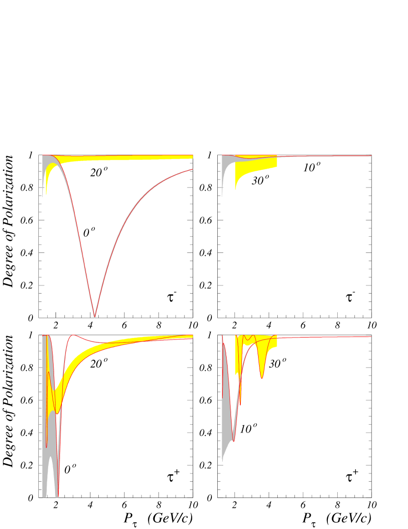
Figure 1: Degree of polarization, $\left|\boldsymbol{\mathcal{P}}\right|$, of $\tau$ leptons produced in reactions $\nu_{\tau}n\to\tau^{-}p$ and $\overline{\nu}_{\tau}p\to\tau^{+}n$, as a function of the lepton momentum for scattering angles $\theta=0^{\circ},10^{\circ},20^{\circ}$ and $30^{\circ}$. The meaning of the curves and filled areas is explained in the text.

The axial SCC contributions are rather responsive to variation of each of the parameters $\xi_{T}$, $M_{T}$ and $\phi_{T}$.

As is seen from the figures, the SCC may essentially affect the polarization vector, particularly at low lepton momenta and large scattering angles; more sizably in case of $\tau^{+}$. However, in the kinematic regions for which the cross section of lepton production is comparatively large, the SCC effects are not too dramatic and (especially in case of $\tau^{+}$) they are more sensitive to small variations of the standard axial and pseudoscalar form factors. This is a disadvantage for experimental investigation of the SCC effects but a clear advantage for the future neutrino oscillation experiments since the relevant uncertainties are not very significant. Recall that our analysis is only valid within the adopted ad hoc model for the SCC induced tensor form factor, including somewhat optional range for the tensor mass values.

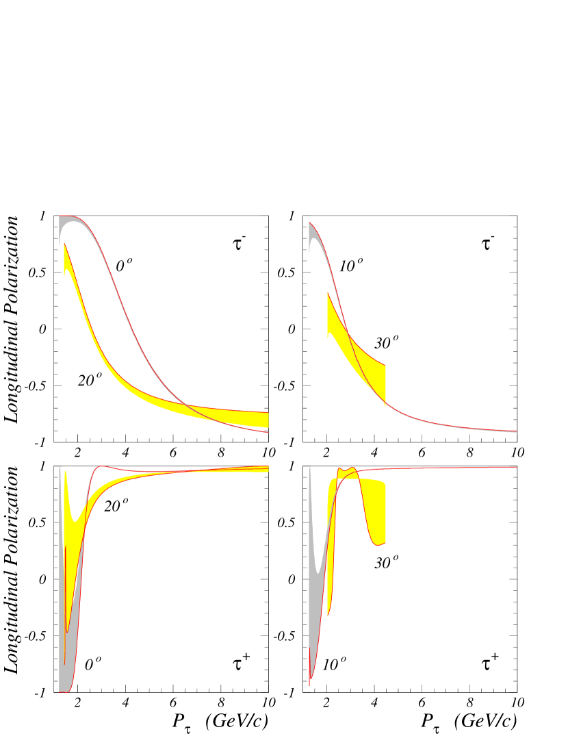
Figure 2: Longitudinal polarization of $\tau^{\pm}$ leptons. The notation is the same as in Fig. 1.

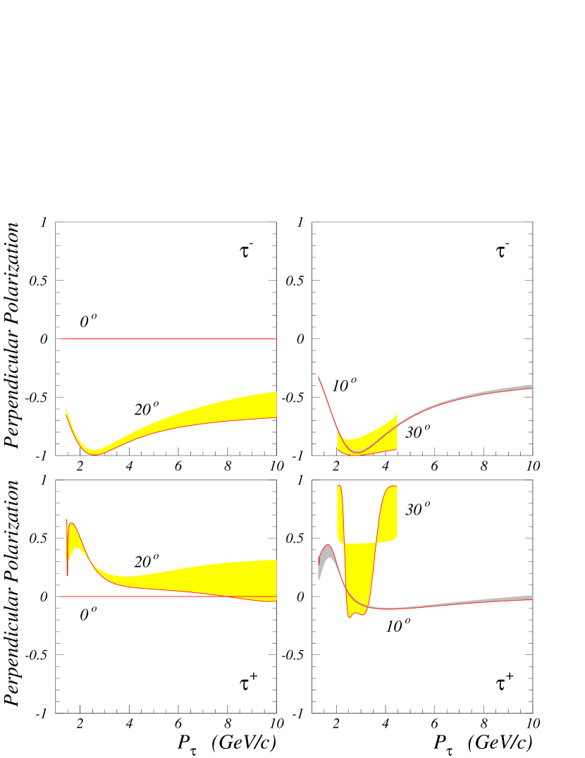
Figure 3: Perpendicular polarization of $\tau^{\pm}$ leptons. The notation is the same as in Fig. 1.

4 SUMMARY

We derived the most general formulas for the structure functions describing the QE production of octet baryons in CC $\nu_{\tau}n$ and $\overline{\nu}_{\tau}p$ interactions; both standard (FCC induced) and nonstandard (SCC induced) contributions were taken into account. As an example of application of our result, we studied the axial SCC effects to the polarization of $\tau$ leptons produced in the $\Delta{Y}=0$ reactions.

References

• [1] K. Hagiwara, K. Mawatari, H. Yokoya, Nucl. Phys. B 668 (2003) 364 (hep-ph/0305324).
• [2] K.S. Kuzmin, V.V. Lyubushkin, V.A. Naumov, in Proc. of “SPIN-03”, Dubna, 16–20 September, 2003 (hep-ph/0312107).
• [3] K.S. Kuzmin, V.V. Lyubushkin, V.A. Naumov, in Proc. of “SCYSS-04”, Dubna, 2–6 February, 2004 (hep-ph/0403110).
• [4] K. Hagiwara, K. Mawatari, H. Yokoya, Phys. Lett. B 591 (2004) 113 (hep-ph/0403076); C. Bourrely, J. Soffer, O.V.Teryaev, Phys. Rev. D 69 (2004) 114019 (hep-ph/0403176); K.M. Graczyk, hep-ph/0407275; see also these proceedings and hep-ph/0407283.
• [5] D.H. Wilkinson, Eur. Phys. J. A 7 (2000) 307; Nucl. Instrum. Meth. A 455 (2000) 656; ibid., A 469 (2001) 286.
• [6] S. Gardner, C. Zhang, Phys. Rev. Lett. 86 (2001) 5666 (hep-ph/0012098).
• [7] C.H. Llewellyn Smith, Phys. Rept. 3 C (1972) 261.
• [8] A. Strumia, F. Vissani, Phys. Lett. B 564 (2003) 42 (astro-ph/0302055).
• [9] E.L. Lomon, Phys. Rev. C 66 (2002) 045501 (nucl-th/0203081).
• [10] H. Budd, A. Bodek, J. Arrington, hep-ex/0308005; see also these proceedings.
• [11] N.J. Baker et al., Phys. Rev. D 23 (1981) 2499; M.J. Murtagh, in Proc. of “Neutrino-81”, Wailea, Hawaii, 1–8 July, 1981, Vol. 2, p. 388 (report BNL-30082); S.V. Belikov et al., Z. Phys. A 320 (1985) 625.
• [12] L.A. Ahrens et al., Phys. Lett. B 202 (1988) 284.