Abstract

Using the most recent determinations of several theoretical and experimental parameters, we update the Unitarity Triangle analysis in the Standard Model. The basic experimental constraints come from the measurements of $\varepsilon_{K}$, $\left|V_{ub}/V_{cb}\right|$, and $\Delta m_{d}$, the limit on $\Delta m_{s}$, and the measurement of the CP asymmetry in the $B$ sector through the $J/\psi K^{0}$ channel. In addition we also include in our analysis the direct determination of $\sin{2\alpha}$, $\gamma$, and $\sin(2\beta+\gamma)$ from the measurements of new CP-violating quantities, recently coming from the B-Factories. We also discuss the opportunities offered by improving the precision of the measurements of the various physical quantities entering in the determination of the Unitarity Triangle parameters.
The results and the plots presented in this paper can be also found at the URL http://www.utfit.org, where they are continuously updated with the newest experimental and theoretical results [1].

1 Introduction

The analysis of the Unitarity Triangle (UT) and CP violation represents one of the most stringent tests of the Standard Model (SM) and, for this reason, it is also an interesting window on New Physics (NP). The most precise determination of the parameters governing this phenomenon is obtained using B decays, $\rm{B^{0}}-\overline{\rm{B}^{0}}$ oscillations and CP asymmetries in the kaon and in the B sectors.

Up to now, the standard analysis [2, 3] relies on the following measurements: $\left|V_{ub}\right|/\left|V_{cb}\right|$, $\Delta{m_{d}}$, the limit on $\Delta{m_{s}}$, and the measurements of CP-violating quantities in the kaon ($\varepsilon_{K}$) and in the B ($\sin{2\beta}$) sectors. Inputs to this analysis constitute a large body of both experimental measurements and theoretically determined parameters, where Lattice QCD calculations play a central role. A careful choice (and a continuous update) of the values of these parameters is a prerequisite in this study. The values and errors attributed to these parameters are summarized in Table 1 (Section 2).
The results of the analysis and the determination of the UT parameters are presented and discussed in Section 3 which is an update of similar analyses performed in [2] to which the readers can refer for more details.
New CP-violating quantities have been recently measured by the B-Factories, allowing for the determination of several combinations of UT angles. The measurements of sin2$\alpha$, $\gamma$, and $\sin(2\beta+\gamma)$ are now available using B decays into $\pi\pi$ and $\rho\rho$, D^(∗)K and D${}^{(*)}\pi$ final states, respectively. These measurements are presented in Section 4 and their effect on the UT fit is discussed in Section 4.4.
Finally we also discuss the perspectives opened by improving the precision in the measurements of various physical quantities entering the UT analysis. In particular, we investigate to which extent future and improved determinations of the experimental constraints, such as sin2$\beta$, $\Delta m_{s}$ and $\gamma$, could allow us to invalidate the SM, thus signaling the presence of NP effects.

2 Inputs used for the “Standard” analysis

The values and errors of the relevant quantities entering the standard analysis of the CKM parameters (corresponding to the constraints from $\left|V_{ub}\right|/\left|V_{cb}\right|$, $\Delta{m_{d}}$, $\Delta{m_{s}}/\Delta{m_{d}}$, $\varepsilon_{K}$ and $\sin{2\beta}$) are summarized in Table 1.
The novelties here are the final LEP/SLD likelihood from $\Delta m_{s}$, the value of $|V_{ub}|$ from inclusive semileptonic decays [4], the new value of $\sin{2\beta}$ and a new treatment of the non-perturbative QCD parameters as explained in the following section 2.1.

Parameter	Value	Gaussian ($\sigma$)	Uniform
			(half-width)
$\lambda$	0.2265	0.0020	-
$\left|V_{cb}\right|$(excl.)	$42.1\times 10^{-3}$	$2.1\times 10^{-3}$	-
$\left|V_{cb}\right|$(incl.)	$41.4\times 10^{-3}$	$0.7\times 10^{-3}$	$0.6\times 10^{-3}$
$\left|V_{ub}\right|$(excl.)	$33.0\times 10^{-4}$	$2.4\times 10^{-4}$	$4.6\times 10^{-4}$
$\left|V_{ub}\right|$(incl.-LEP)	$40.9\times 10^{-4}$	$6.2\times 10^{-4}$	$4.7\times 10^{-4}$
$\left|V_{ub}\right|$(incl.-HFAG)	$45.7\times 10^{-4}$	$6.1\times 10^{-4}$	-
$\Delta m_{d}$	$0.503~{}\mbox{ps}^{-1}$	$0.006~{}\mbox{ps}^{-1}$	-
$\Delta m_{s}$	$>$ 14.5 ps-1 at 95% C.L.	sensitivity 18.3 ps-1
$m_{t}$	$167$ GeV	$5$ GeV	-
$f_{B_{s}}\sqrt{\hat{B}_{B_{s}}}$	$276$ MeV	$38$ MeV	-
$\xi=\frac{f_{B_{s}}\sqrt{\hat{B}_{B_{s}}}}{f_{B_{d}}\sqrt{\hat{B}_{B_{d}}}}$	1.24	0.04	$\pm$ 0.06
$\eta_{b}$	0.55	0.01	-
$\hat{B}_{K}$	0.86	0.06	0.14
$\varepsilon_{K}$	$2.280\times 10^{-3}$	$0.013\times 10^{-3}$	-
$\eta_{1}$	1.38	0.53	-
$\eta_{2}$	0.574	0.004	-
$\eta_{3}$	0.47	0.04	-
$f_{K}$	0.159 GeV	fixed
$\Delta m_{K}$	0.5301 $\times 10^{-2}~{}\mbox{ps}^{-1}$	fixed
$\sin{2\beta}$	0.739	0.048	-
$m_{b}$	4.21 GeV	0.08 GeV	-
$m_{c}$	1.3 GeV	0.1 GeV	-
$\alpha_{s}$	0.119	0.03	-
$G_{F}$	1.16639 $\times 10^{-5}\rm{GeV}^{-2}$	fixed
$m_{W}$	80.22 GeV	fixed
$m_{B^{0}_{d}}$	5.279 GeV	fixed
$m_{B^{0}_{s}}$	5.375 GeV	fixed
$m_{K}$	0.493677 GeV	fixed

Table 1: Values of the relevant quantities used in the fit of the CKM parameters. In the third and fourth columns the Gaussian and the flat contributions to the uncertainty are given respectively (for details on the statistical treatment see [2]). The central values and errors are those adopted at the end of the “CKM Unitarity Triangle” Workshops ([5], [6]) and by the HFAG [4].

2.1 Use of $\xi$, $f_{B_{s}}\sqrt{\hat{B}_{B_{s}}}$ and $f_{B_{d}}\sqrt{\hat{B}_{B_{d}}}$ in $\Delta m_{s}$ and $\Delta m_{d}$ constraints

One of the important differences with respect to previous studies is in the use of the information from non-perturbative QCD parameters entering the expressions of $\Delta m_{s}$ and $\Delta m_{d}$. The ${\rm B}^{0}_{s}-\overline{\rm{B}^{0}_{s}}$ time oscillation frequency, which can be related to the mass difference between the light and heavy mass eigenstates of the ${\rm B}^{0}_{s}-\overline{{\rm B}^{0}_{s}}$ system, is proportional to the square of the $|V_{ts}|$ element. Up to Cabibbo suppressed corrections, $|V_{ts}|$ is independent of $\overline{\rho}$ and $\overline{\eta}$. As a consequence, the measurement of $\Delta m_{s}$ would provide a strong constraint on the non-perturbative QCD parameter $f_{B_{s}}^{2}\hat{B}_{B_{s}}$.
For this reason we propose a new and more appropriate way of treating the constraints coming from the measurements of $\Delta m_{s}$ and $\Delta m_{d}$. In previous analyses, these constraints were implemented using the following equations:

$$\Delta m_{d} \propto [(1-\overline{\rho})^{2}+\overline{\eta}^{2}]f_{B_{d}}^{2}\hat{B}_{B_{d}}$$ (1)

$$\Delta m_{s} \propto f_{B_{s}}^{2}\hat{B}_{B_{s}}=f_{B_{d}}^{2}\hat{B}_{B_{d}}\times\xi^{2}$$

where $\xi=f_{B_{s}}\sqrt{\hat{B}_{B_{s}}}/f_{B_{d}}\sqrt{\hat{B}_{B_{d}}}$. In this case the input quantities are $f_{B_{d}}\sqrt{\hat{B}_{B_{d}}}$ and $\xi$. The constraints from $\Delta m_{s}$ and the knowledge of $\xi$ are used to improve the knowledge on $f_{B_{d}}\sqrt{\hat{B}_{B_{d}}}$ which thus makes the constraint on $\Delta m_{d}$ more effective. The main problem of this method is that the quantity that we know best from Lattice calculations is $f_{B_{s}}^{2}\hat{B}_{B_{s}}$, whereas $\xi^{2}$ and $f_{B_{d}}^{2}\hat{B}_{B_{d}}$ are affected by large uncertainties coming from chiral extrapolations. We thus suggest to use a different method which consists in writing the constraints in the following way:

$$\Delta m_{d} \propto [(1-\overline{\rho})^{2}+\overline{\eta}^{2}]\frac{f_{B_{s}}^{2}\hat{B}_{B_{s}}}{\xi^{2}}$$ (2)

$$\Delta m_{s} \propto f_{B_{s}}^{2}\hat{B}_{B_{s}}$$

At present, this new parameterization does not have a large effect on final results but, in the future, the measurement of $\Delta m_{s}$ will allow the elimination of a further theoretical parameter, $f_{B_{s}}^{2}\hat{B}_{B_{s}}$, from the UT fits. To obtain a more effective constraint on $\Delta m_{d}$, also the error on $\xi$ should be improved.

3 Determination of the Unitarity Triangle parameters

In this section, assuming the validity of the Standard Model, we give the results for the quantities defining the Unitarity Triangle: $\overline{\rho}$, $\overline{\eta}$, $\sin{2\beta}$, $\sin{2\alpha}$, $\gamma$, sin$(2\beta+\gamma)$ as well as other quantities such as $\Delta m_{s}$, $f_{B_{s}}\sqrt{\hat{B}_{B_{s}}}$, $\hat{B}_{K}$ and $\xi$. The inputs are summarized in Table 1.

3.1 Fundamental test of the Standard Model in the fermion sector

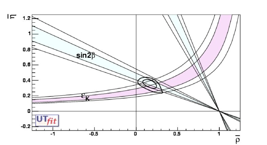
Figure 1: The allowed regions for $\overline{\rho}$ and $\overline{\eta}$ (contours at 68%, 95% probability ranges), as selected by the measurements of $\left|V_{ub}\right|/\left|V_{cb}\right|$, $\Delta{m_{d}}$, and by the limit on $\Delta{m_{s}}/\Delta{m_{d}}$, are compared with the bands (at 68% and 95% probability ranges) from the measurements of CP-violating quantities in the kaon ($\varepsilon_{K}$) and in the B ($\sin{2\beta}$) sectors.

The most crucial test consists in the comparison between the ($\overline{\rho}-\overline{\eta}$) region selected by the measurements which are sensitive only to the sides of the Unitarity Triangle (semileptonic B decays and ${\rm B}^{0}-\overline{{\rm B}^{0}}$ oscillations) and the regions selected by the direct measurements of CP violation in the kaon ($\varepsilon_{K}$) or in the B ($\sin{2\beta}$) sectors. This test is shown in Figure 1. It can be translated quantitatively through the comparison between the value of $\sin{2\beta}$ obtained from the measurement of the CP asymmetry in $J/\psi K^{0}$ decays and the one determined from “sides” measurements:

$$\sin{2\beta}= 0.724\pm 0.049~{}[0.613;0.803]~{}{\rm at}~{}95\%~{}C.L. ~{}~{}\rm{sides~{}only}$$

$$\sin{2\beta}= 0.739\pm 0.048~{}[0.681;0.787]~{}{\rm at}~{}95\%~{}C.L. ~{}~{}\rm J/\psi K^{0}.$$ (3)

The spectacular agreement between these values illustrates the consistency of the Standard Model in describing CP violation phenomena in terms of one single parameter $\overline{\eta}$. It is also an important test of the Operator Product Expansion (OPE), the Heavy Quark Effective Theory (HQET) and Lattice QCD (LQCD) which have been used to extract the CKM parameters. It has to be noted that this test is even more significant because the errors on $\sin{2\beta}$ from the two determinations are comparable.

As a matter of fact, the value of $\sin{2\beta}$ was predicted, before its first direct measurement was obtained, by using all other available constraints, ($\left|V_{ub}\right|/\left|V_{cb}\right|$, $\varepsilon_{K}$, $\Delta m_{d}$ and $\Delta m_{s}$). The “indirect” determination has improved regularly over the years. Figure 2 shows this evolution for the “indirect” determination of sin2$\beta$ which is compared with the recent determinations of $\sin{2\beta}$ from direct measurements.

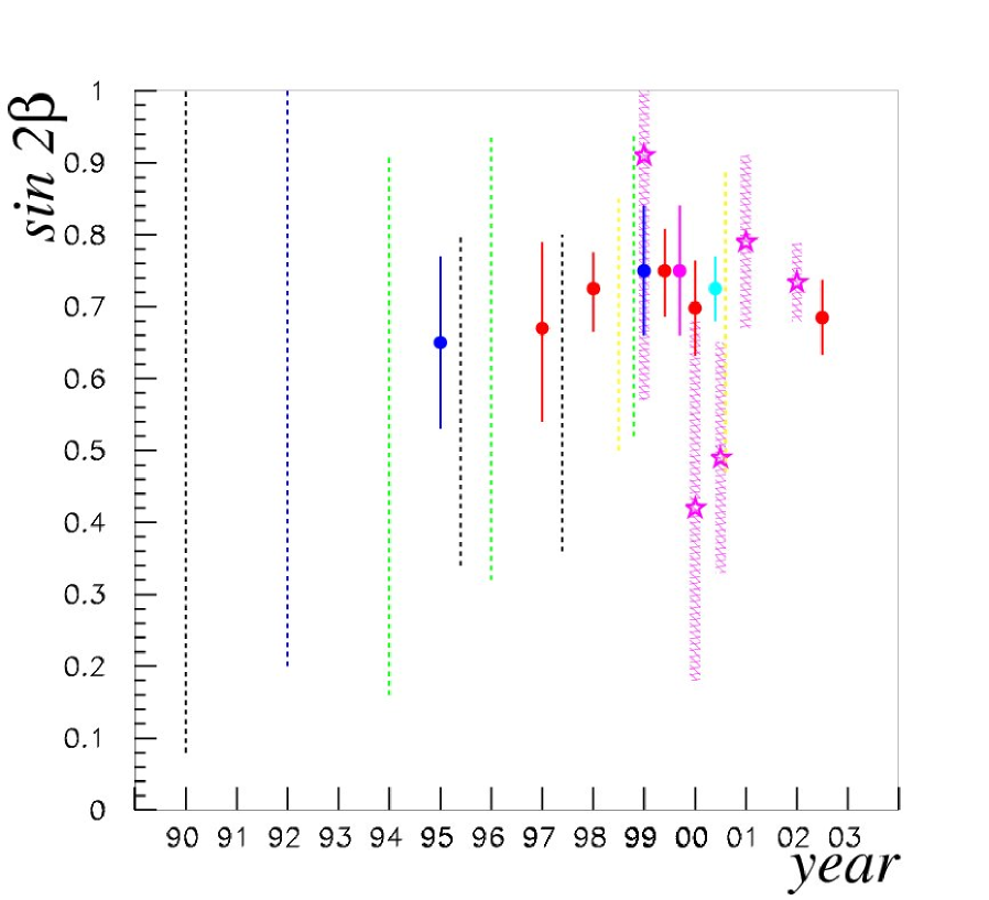
Figure 2: Evolution of the “indirect” determination of $\sin{2\beta}$ over the years (until 2003). From left to right, they correspond to the following papers [3, 7]: DDGN90, LMMR92, AL94, CFMRS95, BBL95, AL96, PPRS97, BF97, BPS98, PS98, AL99, CFGLM99, CPRS99, M99, CDFLMPRS00, B.et.al.00, HLLL00 and CFLPSS [2]. The dotted lines correspond to the 95$\%$ C.L. regions (the only information given in those papers). The larger bands (from year ’99) correspond to values of $\sin{2\beta}$ from direct measurements ($\pm 1\sigma$).

3.2 Determination of the Unitarity Triangle parameters

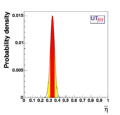
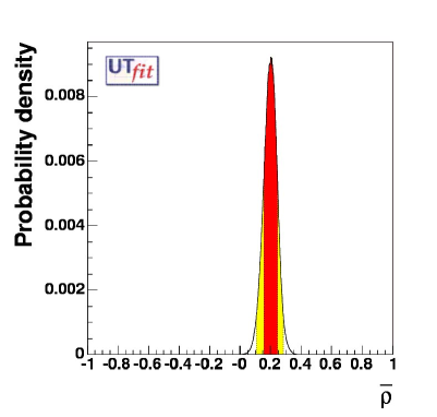
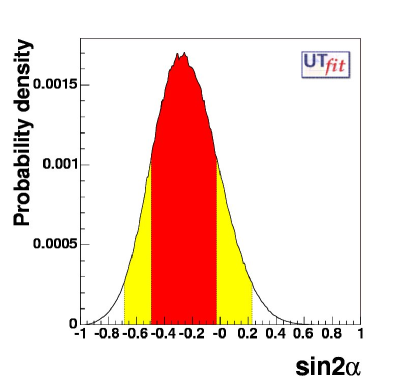
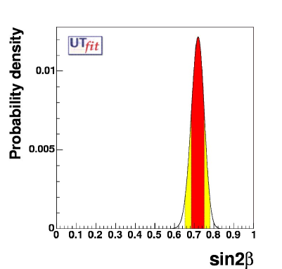
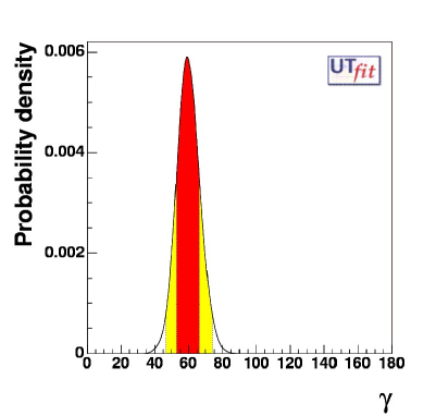
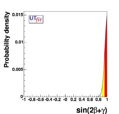
Figure 3: From top left to bottom, the p.d.f.’s for $\overline{\eta}$, $\overline{\rho}$, $\sin{2\alpha}$, $\sin{2\beta}$, $\gamma$ and $\sin(2\beta+\gamma)$. The red (darker) and the yellow (lighter) zones correspond respectively to 68% and 95% of the normalised area. The following contraints have been used: $\left|V_{ub}\right|/\left|V_{cb}\right|$, $\varepsilon_{K}$, $\Delta m_{d}$, $\Delta m_{s}$ and $\sin{2\beta}$ from the measurement of the CP asymmetry in the $J/\psi K^{0}$ decays.

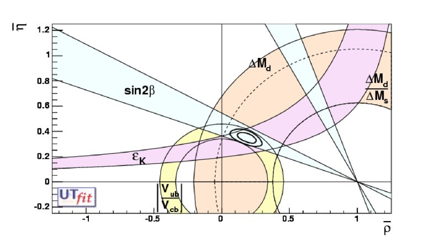
Figure 4: Allowed regions for $\overline{\rho}$ and $\overline{\eta}$ using the parameters listed in Table 1. The closed contours at 68% and 95% probability are shown. The full lines correspond to 95% probability regions for the constraints, given by the measurements of $\left|V_{ub}\right|/\left|V_{cb}\right|$, $\varepsilon_{K}$, $\Delta m_{d}$, $\Delta m_{s}$ and $\sin{2\beta}$ from the measurement of the CP asymmetry in the $J/\psi K^{0}$ decays.

Using the constraints from $\left|V_{ub}\right|/\left|V_{cb}\right|$, $\Delta{m_{d}}$, $\Delta{m_{s}}/\Delta{m_{d}}$, $\varepsilon_{K}$ and $\sin{2\beta}$, we obtain the results given in Table 2.

Parameter	68$\%$	95$\%$	99$\%$
$\overline{\eta}$	0.348 $\pm$ 0.028	[0.293;0.403]	[0.275;0.418]
$\overline{\rho}$	0.172 $\pm$ 0.047	[0.082;0.270]	[0.051;0.302]
$\sin{2\beta}$	0.725 $\pm$ 0.033	[0.645;0.772]	[0.627;0.793]
$\sin{2\alpha}$	-0.16 $\pm$ 0.26	[-0.62;0.35]	[-0.75;0.48]
$\gamma[^{\circ}$]	61.5 $\pm$ 7.0	[47.5;76.6]	[43.3;81.6]
$\sin(2\beta+\gamma)$	$>0.94$	$>0.88$	$>0.84$
$Im{\lambda}_{t}$[$10^{-5}$]	13.5 $\pm$ 1.0	[11.5;15.3]	[10.8;15.9]

Table 2: Values and probability ranges for the Unitarity Triangle parameters obtained by using the following constraints: $\left|V_{ub}\right|/\left|V_{cb}\right|$, $\Delta{m_{d}}$, $\Delta{m_{s}}/\Delta{m_{d}}$, $\varepsilon_{K}$ and $\sin{2\beta}$.

Figures 3 and 4 show, respectively, the p.d.f.’s for the main Unitarity Triangle parameters and the selected region in the $\overline{\rho}-\overline{\eta}$ plane.

3.3 Determination of other important quantities

In the previous sections we have shown that it is possible to obtain the p.d.f.’s for all the various UT parameters. It is instructive to remove from the fitting procedure the external information on the value of one (or more) of the constraints.

In this section we study the distributions of $\Delta m_{s}$ and of the hadronic parameters. For instance, in the case of the hadronic parameters, it is interesting to remove from the fit the constraints on their values coming from lattice calculations and use them as one of the free parameters of the fit. In this way we may compare the uncertainty obtained on a given quantity through the UT fit to the present theoretical error on the same quantity.

3.3.1 The expected distribution for $\Delta m_{s}$

Removing the constraint coming from $\Delta m_{s}$, the probability distribution for $\Delta m_{s}$ itself can be extracted as shown in Figure 5. The results of this exercise are given in Table 3. Present analyses at LEP/SLD have established a sensitivity of 18.3 ps^-1 and they show a higher probability region for a positive signal (see left plot in Fig. 5: a “signal bump” appears around 17.5 ps^-1) well compatible with the range of the $\Delta m_{s}$ distribution from the UT fit (see right plot in Fig. 5). Accurate measurements of $\Delta m_{s}$ are expected from the TeVatron in the next future.

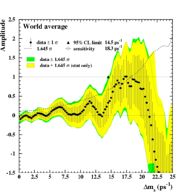
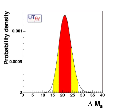
Figure 5: Left plot: combined results [4] from all analyses on the oscillation amplitude, as a function of $\Delta{m}_{s}$. The points with error bars are the data; the lines show the 95% C.L. curves (in dark the systematics have been included). The dotted curve corresponds to the sensitivity. Right plot: $\Delta m_{s}$ probability distributions, obtained without using the information from ${\rm B}^{0}_{s}-\overline{{\rm B}^{0}_{s}}$ mixing.

Parameter	68$\%$	95$\%$	99$\%$
$\Delta m_{s}$(including  $\Delta m_{s}$) [ps-1]	18.3 $\pm$ 1.6	(15.4-23.1)	(15.1-27.0)
$\Delta m_{s}$(without $\Delta m_{s}$) [ps-1]	21.1 $\pm$ 3.1	(15.3-27.7)	(13.7-29.9)

Table 3: Central values and ranges for $\Delta m_{s}$ corresponding to defined levels of probability, obtained by including or not including the information from the experimental amplitude spectrum ${\cal A}(\Delta m_{s})$.

3.3.2 Determination of $f_{B_{s}}\sqrt{\hat{B}_{B_{s}}}$, $\hat{B}_{K}$ and $\xi$

To obtain the p.d.f. for a given quantity, we perform the UT fit imposing as input a uniform distribution of the quantity itself in a range much wider than the expected interval of values assumed by the parameter. Table 4 shows the results of the UT fit when one parameter at the time is taken out of the fit with this procedure (see Figure 6). The central value and the error of each of these quantities has to be compared to the current evaluation from lattice QCD, given in Table 1.

Parameter	68$\%$	95$\%$	99$\%$
$\xi$	1.13${}^{+0.12}_{-0.09}$	[0.95;1.41]	[0.92;1.57]
$f_{B_{s}}\sqrt{\hat{B}_{B_{s}}}$(MeV)	263 $\pm$ 14	[236;290]	[231;320]
$\hat{B}_{K}$	0.65 $\pm$ 0.10	[0.49;0.87]	[0.45;0.99]

Table 4: Values and probability ranges for the non-perturbative QCD parameters, if the external information (input) coming from the theoretical calculation of these parameters is not used in the CKM fits.

Some conclusions can be drawn. The precision on $f_{B_{s}}\sqrt{\hat{B}_{B_{s}}}$ obtained from the fit has an accuracy which is better than the current evaluation from lattice QCD. This proves that the standard CKM fit is, in practice, weakly dependent on the assumed theoretical uncertainty on $f_{B_{s}}\sqrt{\hat{B}_{B_{s}}}$.

The result on $\hat{B}_{K}$ indicates that values of $\hat{B}_{K}$ smaller than $0.45$ are excluded at $99\%$ probability, while large values of $\hat{B}_{K}$ are compatible with the prediction coming from the UT fit using the other constraints. The present estimate of $\hat{B}_{K}$ from lattice QCD, which has a 15$\%$ relative error (Table 1), is still more precise than the indirect determination from the UT fit. Likewise, the present best determination of the parameter $\xi$ comes from lattice QCD.

In the above exercise we have removed from the UT fit individual quantities one by one. It is also interesting to see what can be obtained taking out two of them simultaneously. Figures 6 show the regions selected in the planes ($f_{B_{s}}\sqrt{\hat{B}_{B_{s}}}$, $\hat{B}_{K}$), ($\xi$, $\hat{B}_{K}$) and ($f_{B_{s}}\sqrt{\hat{B}_{B_{s}}}$, $\xi$). The corresponding results are summarized in Table 5.

Parameter	68$\%$	95$\%$	99$\%$
$f_{B_{s}}\sqrt{\hat{B}_{B_{s}}}$(MeV)	252 $\pm$ 13	[228;283]	[219;325]
$\hat{B}_{K}$	0.63$\pm$ 0.10	[0.48;0.87]	[0.44;1.02]
$f_{B_{s}}\sqrt{\hat{B}_{B_{s}}}$(MeV)	-	$>0.23$	$>0.22$
$\xi$	-	$>0.98$	$>0.92$
$\hat{B}_{K}$	$0.53^{+0.19}_{-0.07}$	[0.41,0.99]	[0.39,1.18]
$\xi$	1.33 $\pm$ 0.20	[0.99,1.63]	[0.95,1.70]

Table 5: Values and probability ranges for the non-perturbative QCD parameters, if two external pieces of information (inputs) coming from the theoretical calculation of these parameters are not used in the CKM fits.

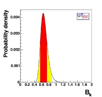
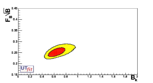
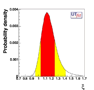
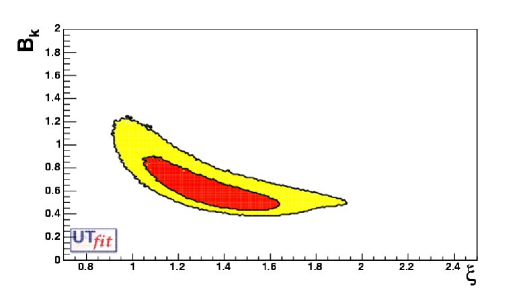
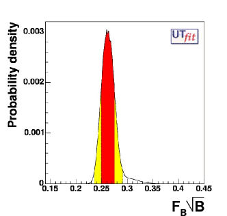
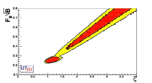
Figure 6: One- and two-dimensional 68% and 95% probability distributions for $\hat{B}_{K}$, $\xi$ and $f_{B_{s}}\sqrt{\hat{B}_{B_{s}}}$ (see Sec. 3.3.2).

4 New Constraints from UT angle measurements

The values for $\sin{2\alpha}$, $\gamma$, and $\sin(2\beta+\gamma)$ given in Table 2 have to be taken as predictions for future measurements. A strong message is given for instance for the angle $\gamma$. Its indirect determination is known with an accuracy of about $10\%$. It has to be stressed that, with present measurements, the probability for $\gamma$ to be greater than $90^{\circ}$ is only $0.0055\%$.

Thank to the huge statistics collected at the B-Factories, new CP-violating quantities have been recently measured allowing for the direct determination of $\sin{2\alpha}$, $\gamma$, and $\sin(2\beta+\gamma)$. In the following we present the UT fit results including these new measurements and their impact on the $\overline{\rho}-\overline{\eta}$ plane.

4.1 Determination of the angle $\gamma$ using DK events

Various methods using $B\rightarrow DK$ decays have been used to determine the Unitarity Triangle angle $\gamma$ [8]. The basic idea in these methods is the following. A charged $B^{-}$ can decay into a $D^{0}(\overline{D}^{0})K^{-}$ final state via a $V_{cb}$($V_{ub})$ mediated process. CP violation occurs if the $D^{0}$ and the $\overline{D}^{0}$ decay in the same final state. The measurement of the direct CP violation is thus sensitive to the $V_{ub}$ and $V_{cb}$ phase difference, $\gamma$. The same argument can be applied to $B\rightarrow D^{*}K$ decays.
The most important aspect of these decays is that they proceed only via tree-level diagrams, implying that the determination of $\gamma$ is not affected by possible New Physics loop contributions.

One of these methods is the “GLW method” and it consists in reconstructing $D^{0}$ mesons in a specific CP (even/odd) mode. The “ADS method” is, instead, based on the fact that $D^{0}(\overline{D}^{0})$ decays can reach the same final state through Doubly Cabibbo Suppressed (DCS) (Cabibbo Allowed (CA)) processes. The following observables are defined in these two methods:

$$R_{C\!P^{+}} = 1+r_{B}^{2}-2r_{B}\sin\gamma\sin\delta_{B}$$ (4)

$$R_{C\!P^{-}} = 1+r_{B}^{2}-2r_{B}\sin\gamma\cos\delta_{B}$$

$$A_{C\!P^{+}} = 2r_{B}\sin\gamma\sin\delta_{B}/R_{C\!P^{+}}$$

$$A_{C\!P^{-}} = -2r_{B}\sin\gamma\sin\delta_{B}/R_{C\!P^{-}}$$

$$R_{ADS} = r_{DCS}^{2}+r_{B}^{2}+2r_{B}r_{DCS}\cos\gamma\cos(\delta_{B}~{}+~{}\delta_{D})$$

where

$$r_{B}=\frac{{\cal A}(B^{-}\rightarrow D^{0}K^{-})}{{\cal A}(B^{-}\rightarrow\overline{D}^{0}K^{-})},$$ (5)

$r_{DCS}=\sqrt{\frac{D^{0}\rightarrow K^{+}\pi^{-}}{D^{0}\rightarrow K^{-}\pi^{+}}}$ and $\delta_{B}$ ($\delta_{D}$) is the difference between the strong phases of the two amplitudes in the B system (B and D systems).
In [9] a new method based on the Dalitz analysis of three-body decays has been proposed and recent results using this new technique applied to the $D^{0}\rightarrow K_{s}\pi^{-}\pi^{+}$ decays have been published by the Belle Collaboration [10]. The advantage of this method is that the full sub-resonance structure of the three-body decay is considered, including interferences such as those used for GLW and ADS methods plus additional interferences because of the overlap of broad resonances in certain regions of the Dalitz plot. The same analysis can also be performed using $B\rightarrow D^{*0}K$ decays. The technique is identical to the one used in $B\rightarrow D^{0}K$ decays but the values for $r_{B}$ and $\delta_{B}$ are different so they will be indicated as $r^{*}_{B}$ and $\delta^{*}_{B}$ in the following. It is also interesting to note that the Dalitz analysis has only a two-fold discrete ambiguity ($\gamma+\pi,\gamma-\pi$) and not a four-fold ambiguity as in case of the GLW and ADS methods. It has to be noted that experimental likelihoods have been used to correctly implement the measurement of $R_{ADS}$ and the Dalitz result.
A summary of the experimental results is given in Table 6.

Observable	World Average
$A_{C\!P^{+}}$	0.07 $\pm$ 0.13
$A_{C\!P^{-}}$	-0.19 $\pm$ 0.18
$R_{C\!P^{+}}$	1.09 $\pm$ 0.16
$R_{C\!P^{-}}$	1.30 $\pm$ 0.25
$R_{ADS}$	0.0054 $\pm$ 0.0124
$r_{B}(r_{B}^{*})$	$0.26^{+0.10}_{-0.14}\pm 0.03\pm 0.04$ ($0.20^{+0.19}_{-0.17}\pm 0.02\pm 0.04$)
$\gamma$	$77^{+19}_{-17}\pm 13\pm 11$ (Belle Dalitz)

Table 6: Summary of the results obtained with $B\rightarrow D^{(*)}K$ decays and using the GLW and the ADS methods. The last two lines give the results from the Dalitz analysis [9], for which the ambiguity $\gamma\to\pi-\gamma$ is implicit.

All measurements in Table 6 are used to extract $\gamma$. The p.d.f.’s of $\gamma$, $r_{B}$ ($r^{*}_{B}$) and the selected region in the $\gamma$ vs $r_{B}$ plane are shown in Figure 7, where also the effect of this measurement in the $\overline{\rho}-\overline{\eta}$ plane is shown.

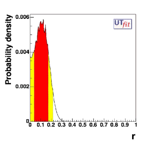
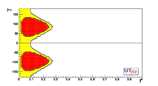
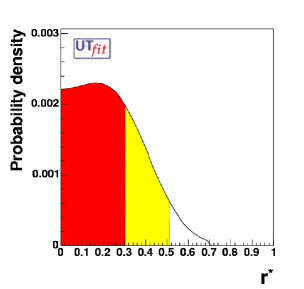
Figure 7: P.d.f.’s for $r_{b}$ from DK (top-left), for $r^{*}_{b}$ from D^∗K (center-left) and for $\gamma$ (bottom-left) using the results from $B\rightarrow D^{(*)}K$ decays. The plots on the right show the measurement of the angle $\gamma$ in the $r^{(*)}_{b}-\gamma$ (top, center) and $\overline{\rho}-\overline{\eta}$ (bottom) planes.

The comparison between the direct and the indirect determination is:

$$\gamma[^{\circ}] = 61.5\pm 7.0~{}[47.5;76.6]~{}{\rm at}~{}95\%~{}C.L.~{}~{}\rm{indirect}$$

$$\gamma[^{\circ}] = 73\pm 27~{}[4;133]~{}~{}{\rm at}~{}95\%~{}C.L.(-107\pm 27~{}~{}[-176;-47])~{}\rm{direct}$$ (6)

An important result of this analysis is also the p.d.f. for $r_{B}$ from which the following result can be given:

$$r_{B} = 0.105\pm 0.065~{}[~{}<~{}0.22]~{}{\rm at}~{}95\%~{}C.L.~{}~{}\rm{direct~{}from~{}}DK.$$ (7)

4.2 Determination of sin2$\alpha$ using $\pi\pi$ and $\rho\rho$ events

In the absence of contributions from penguin diagrams, the measurements of the parameter S of the time-dependent CP asymmetry for $B^{0}\to\pi^{+}\pi^{-}$ and $B^{0}\to\rho^{+}\rho^{-}$ give measurements of the quantity sin(2$\alpha$). Even in presence of penguins, one can use the SU(2) flavour symmetry to connect the measured value of S$\equiv\sin(2\alpha_{eff})$ to the value of sin(2$\alpha$), constraining the contribution from penguin diagrams using the Branching Fractions and the direct CP asymmetry measurements of all the $B\to\pi\pi$ ($B\to\rho\rho$) decays [11]. The decay amplitudes in the $SU(2)$ limit and neglecting electroweak penguins can be written as:

$$A^{+-} = -Te^{-i\alpha}+Pe^{i\delta_{P}}$$

$$A^{+0} = -\frac{1}{\sqrt{2}}\left[e^{-i\alpha}(T+T_{c}~{}e^{i\delta_{T_{c}}})\right]$$

$$A^{00} = -\frac{1}{\sqrt{2}}\left[e^{-i\alpha}T_{c}~{}e^{i\delta_{T_{c}}}+P~{}e^{i\delta_{P}}\right]\,.$$ (8)

They can be expressed in terms of three independent hadronic amplitudes, the absolute values of which are denoted as $T$, $T_{c}$ and $P$. Similarly, $\delta_{P}$ and $\delta_{T_{c}}$ are the strong phases of $P$ and $T_{c}$, once the phase convention is chosen so that $T$ is real. It should be noted that these parameters are different for $B\to\pi\pi$ and $B\to\rho\rho$ decays. For the $B\to\rho\rho$ decays we have in principle to further double the parameters for the longitudinal and the transverse polarization. On the other hand the experimental measurements are compatible with decays which are fully longitudinally polarized. For this reason, in case of $B\to\rho\rho$, we make the assumption of fitting the amplitude with only one set of parameters.
Notice that the number of parameters exceeds the number of available measurements. Nevertheless, one can still extract information on $\alpha$, in the same spirit of the bounds à la Grossman-Quinn.
Using the experimental measurements given in Table 7, we thus constrain all these parameters and the value of the UT angle $\alpha$.

$\pi\pi$ $\rho\rho$ Observable BaBar Belle Average BaBar Belle Average C -0.19 $\pm$ 0.20 -0.58 $\pm$ 0.17 -0.46 $\pm$ 0.13 -0.23 $\pm$ 0.28 -0.23 $\pm$ 0.28 S -0.40 $\pm$ 0.22 -1.00 $\pm$ 0.22 -0.74 $\pm$ 0.16 -0.19 $\pm$ 0.35 -0.19 $\pm$ 0.35 $BR^{+-}(10^{-6})$ 4.7 $\pm$ 0.6 4.4 $\pm$ 0.7 4.6 $\pm$ 0.4 30.0 $\pm$ 6.0 30.0 $\pm$ 6.0 $BR^{+0}(10^{-6})$ 5.5 $\pm$ 1.2 5.0 $\pm$ 1.3 5.2 $\pm$ 0.8 22.5 $\pm$ 8.1 31.7 $\pm$ 9.8 26.4 $\pm$ 6.4 $BR^{00}(10^{-6})$ 2.1 $\pm$ 0.7 1.6 $\pm$ 0.6 1.9 $\pm$ 0.5 0.6 $\pm$ 0.8 0.6 $\pm$ 0.8

Table 7: Experimental inputs from Isospin Analysis in $B\to\pi\pi$ and $B\to\rho\rho$ decays [4]. The $B\to\rho\rho$ decays are assumed to be fully polarized, in agreement with available measurements.

In Figure 8 we show the results in terms of $\sin{2\alpha}$ and of the allowed region in the $\overline{\rho}-\overline{\eta}$ plane, from BaBar measurements only and using the world average. It has to be noted that the unphysical value found by Belle has a strong impact on the selected area. On the other hand, the leading contribution is given by $B\to\rho\rho$ decays.

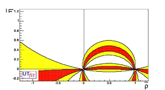
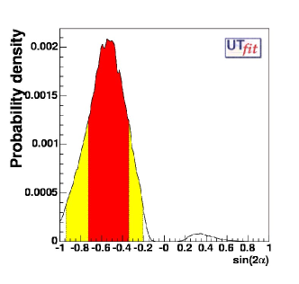
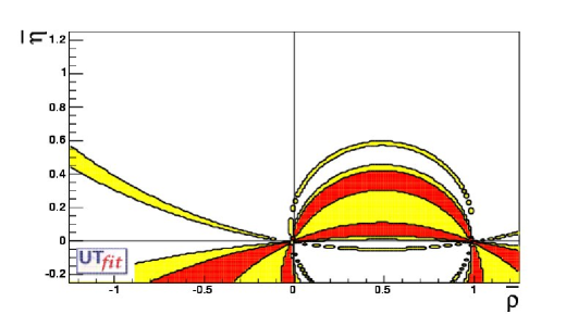
Figure 8: Distribution of sin(2$\alpha$) (left) and relative bound on $\overline{\rho}-\overline{\eta}$ plane (right), using BaBar only (top) and World Average (bottom) [4] values.

The result we get can be compared to the indirect determination from the standard fit:

$$\sin{2\alpha} = -0.16\pm 0.26~{}[-0.62;0.35]~{}{\rm at}~{}95\%~{}C.L.~{}~{}\rm{indirect}$$

$$\sin{2\alpha} = -0.24^{(+0.19)}_{(-0.24)}~{}[-0.75;0.26]~{}{\rm at}~{}~{}95\%~{}C.L.~{}~{}\rm{\pi\pi~{}and~{}\rho\rho~{}BaBar}$$

$$\sin{2\alpha} = -0.55^{(+0.21)}_{(-0.18)}~{}[-0.94;-0.21]~{}{\rm at}~{}~{}95\%~{}C.L.~{}~{}\rm{\pi\pi~{}and~{}\rho\rho~{}(WA)}.$$ (9)

It is important to stress the fact that the main assumptions we are using here, i.e. the validity of SU(2) flavour symmetry and the absence of E.W. penguins. can be directly tested in this framework comparing the experimental and the fitted values of the Branching Fractions (see Table 8). It is clear that all experimental measurements of $B\to\pi\pi$ are in agreement with the SU(2) assumption. On the contrary, we observe from Table 8 a disagreement between the fitted and the experimental value of $BR(B^{+}\to\rho^{+}\rho^{0})$. This discrepancy is shown in Figure 9 and, if confirmed with increased accuracy, it would point towards a violation of the assumptions on which the parameterization of eqs. (8) is based.

$\pi\pi$ $\rho\rho$ Observable Average UTfit Average UTfit $BR^{+-}(10^{-6})$ 4.6 $\pm$ 0.4 4.6 $\pm$ 0.4 30.0 $\pm$ 6.0 32.1 $\pm$ 5.5 $BR^{+0}(10^{-6})$ 5.2 $\pm$ 0.8 5.2 $\pm$ 0.8 26.4 $\pm$ 6.4 20.5 $\pm$ 4.8 $BR^{00}(10^{-6})$ 1.9 $\pm$ 0.5 1.8 $\pm$ 0.5 0.6 $\pm$ 0.8 0.7 $\pm$ 0.8

Table 8: Comparison of input and output values for the Branching Fractions of $B\to\pi\pi$ and $B\to\rho\rho$ decay modes.

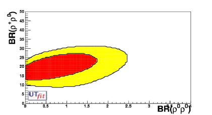
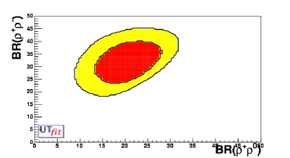
Figure 9: Plots showing the correlation of $BR(B^{+}\to\rho^{+}\rho^{0})$ vs $BR(B^{0}\to\rho^{0}\rho^{0})$(left) and $BR(B^{0}\to\rho^{+}\rho^{-})$ vs $BR(B^{+}\to\rho^{+}\rho^{0})$(right) as obtained from SU(2) parameterizations in UTfit.

4.3 Determination of sin(2$\beta+\gamma$) using $D^{(*)}\pi$ events

$\sin(2\beta+\gamma)$ can be extracted from time-dependent asymmetries in B decays to D^(∗) $\pi$ final states, looking at the interference effects between the decay amplitudes implying $b\rightarrow c$ and $b\rightarrow u$ transitions. The time-dependent rates can be written as:

$$R(B^{0}\rightarrow D^{(*)-}\pi^{+})=N~{}e^{-\Gamma t}~{}{(1+C~{}\cos(\Delta m_{d}t)+S~{}\sin(\Delta m_{d}t)~{})}$$ (10)

$$R(\overline{B}^{0}\rightarrow D^{(*)-}\pi^{+})=N~{}e^{-\Gamma t}~{}{(1-C~{}\cos(\Delta m_{d}t)-S~{}\sin(\Delta m_{d}t)~{})}$$

$$R(B^{0}\rightarrow D^{(*)+}\pi^{-})=N~{}e^{-\Gamma t}~{}{(1+C~{}\cos(\Delta m_{d}t)-\overline{S}~{}\sin(\Delta m_{d}t)~{})}$$

$$R(\overline{B}^{0}\rightarrow D^{(*)+}\pi^{-})=N~{}e^{-\Gamma t}~{}{(1-C~{}\cos(\Delta m_{d}t)+\overline{S}~{}\sin(\Delta m_{d}t)~{})}$$

where S and C parameters are defined as

$$S=2~{}r/(1+r^{2})\sin(2\beta+\gamma-\delta)$$ (11)

$$\overline{S}=2~{}r/(1+r^{2})\sin(2\beta+\gamma+\delta)$$

$$C=(1-r^{2})/(1+r^{2})$$

and r and $\delta$ are the absolute value and the phase of the amplitude ratio $A(\overline{B}^{0}\rightarrow D^{-}\pi^{+})/A(B^{0}\rightarrow D^{-}\pi^{+})$. This ratio $r$ is rather small being of the order of $|V_{ub}/V_{cb}|\simeq$ 0.02.

There is a correlation between the tag side and the reconstruction side in time dependent CP measurements at B-Factories [12]. This is related to the fact that interference between $b\rightarrow c$ and $b\rightarrow u$ transitions in $B\rightarrow DX$ decays can occur also in the tag side. $S$ and $\overline{S}$ entering the time dependent rates can be replaced by

$$a=2r\sin(2\beta+\gamma)\cos(\delta)$$ (12)

$$b=2r^{{}^{\prime}}\sin(2\beta+\gamma)\cos(\delta^{{}^{\prime}})$$

$$c=2\cos(2\beta+\gamma)(r\sin(\delta)-r^{{}^{\prime}}\sin(\delta^{{}^{\prime}}))$$

where $r^{{}^{\prime}}$ and $\delta^{{}^{\prime}}$ are the analogue of $r$ and $\delta$ for the tag side. It is important to stress that this interference on the tag side cannot occur when B mesons are tagged using semileptonic decays. In other words, $r^{{}^{\prime}}$= 0 when only semileptonic decays are considered. In the following we will consider the observables $a$, $c$(lepton), $a^{*}$ and $c^{*}$(lepton), which are functions of $r^{(*)}$, $\delta^{(*)}$ and 2$\beta+\gamma$.

BaBar and Belle provided three different measurements of this channel, with total (both) [13] or partial (BaBar only) [14] reconstruction of the final state, as summarized in Table 9.

Parameters	HFAG average [4]
a	-0.038 $\pm$ 0.021
a∗	0.012 $\pm$ 0.030
c (lepton)	-0.041 $\pm$ 0.029
c∗ (lepton)	-0.015 $\pm$ 0.044

Table 9: Summary of the experimental results from BaBar and Belle, as reported in [4].

We use directly the four experimental quantities: $a^{(*)}$ and $c^{(*)}$(lepton) defined before and we build a global p.d.f. as the product of the p.d.f.’s of these four quantities. We do not make any assumption on $r$ and $r^{*}$ which are extracted in the range [0.0,0.1]. The results on $r$, $r^{*}$, sin(2$\beta+\gamma$) and the impact of this measurement in the $\overline{\rho}-\overline{\eta}$ plane are shown in Figure 10.

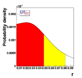
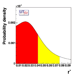
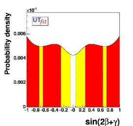
Figure 10: Distributions for $r$ for $D\pi$ (top-left), $r^{*}$ for $D^{*}\pi$ (top-right), $\sin(2\beta+\gamma)$ for $D\pi$ (middle-left), $\sin(2\beta+\gamma)$ for $D^{*}\pi$ (middle-center) and $\sin(2\beta+\gamma)$ combined (middle-right) and bound from $\sin(2\beta+\gamma)$ on the $\overline{\rho}-\overline{\eta}$ plane (bottom).

The comparison between the direct and the indirect determination of sin$(2\beta+\gamma)$ is given below:

$$\sin(2\beta+\gamma) > ~{}~{}0.94~{}~{}{\rm at}~{}68\%~{}C.L.(>0.88~{}{\rm at}~{}95\%~{}C.L.)~{}~{}\rm{indirect}$$

$$\sin(2\beta+\gamma) > ~{}~{}0.28~{}~{}{\rm at}~{}68\%~{}C.L.(>0.08~{}{\rm at}~{}95\%~{}C.L.)~{}~{}\rm D^{(*)}\pi.$$ (13)

4.4 Determination of the Unitarity Triangle parameters using also the new UT angle measurements

It is interesting to see the selected region in $\overline{\rho}-\overline{\eta}$ plane from the measurements of the UT angles in the B sector. The plot is shown in Figure 11. In Table 10 we report the results we get using these constraints.

Figure 11: Allowed regions for $\overline{\rho}$ and $\overline{\eta}$ obtained using the measurements of the UT angles in the B sector: $\sin{2\beta}$, $\sin{2\alpha}$, $\sin(2\beta+\gamma)$ and $\gamma$. The closed contours at $68\%$ and $95\%$ probability are shown. The full zones correspond to $95\%$ probability regions from individual constraints.

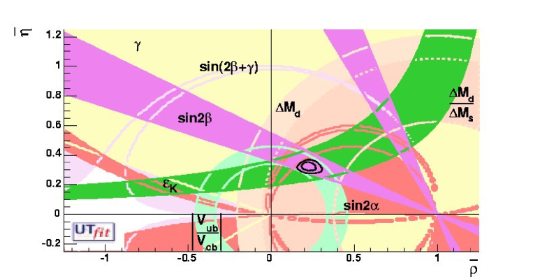
Figure 12: Allowed regions for $\overline{\rho}$ and $\overline{\eta}$ using the parameters listed in Table 1. The closed contours at $68\%$ and $95\%$ probability are shown. The full lines correspond to $95\%$ probability regions for the constraints, given by the measurements of $\left|V_{ub}\right|/\left|V_{cb}\right|$, $\varepsilon_{K}$, $\Delta m_{d}$, $\Delta m_{s}$ and $\sin{2\beta}$,$\gamma$, $\sin(2\beta+\gamma)$ and $\sin{2\alpha}$.

Parameter	68$\%$	95$\%$	99$\%$
$\overline{\eta}$	0.265${}^{+0.120}_{-0.070}$	[0.165;0.869]	[0.052;0.980]
$\overline{\rho}$	0.315${}^{+0.40}_{-0.51}$	[0.040;0.378]	[0.004;0.437]
$\sin{2\beta}$	0.733 $\pm$ 0.049	[0.636;0.828]	[0.606;0.858]
$\sin{2\alpha}$	-0.66 $\pm$ 0.26	$<$0.48	$<$0.59
$\gamma[^{\circ}$]	50.0${}^{+9.2}_{-14.9}$	$<$61.5	$<$79.6
$Im{\lambda}_{t}$[$10^{-5}$]	12.1 $\pm$ 1.6	[5.8,14.3]	[5.1,16.0]

Table 10: Values and probability ranges for the Unitarity Triangle parameters obtained by using $\sin{2\beta}$, $\gamma$, $\sin(2\beta+\gamma)$ and $\sin{2\alpha}$.

The results given in Table 11 are obtained using all the available constraints: $\left|V_{ub}\right|/\left|V_{cb}\right|$, $\Delta{m_{d}}$, $\Delta{m_{s}}/\Delta{m_{d}}$, $\varepsilon_{K}$, $\sin{2\beta}$, $\gamma$, $\sin(2\beta+\gamma)$ and $\sin{2\alpha}$. Figure 12 shows the corresponding selected region in the $\overline{\rho}-\overline{\eta}$ plane.

Parameter	68$\%$	95$\%$	99$\%$
$\overline{\eta}$	0.324 $\pm$ 0.020	[0.283,0.359]	[0.268,0.373]
$\overline{\rho}$	0.225 $\pm$ 0.030	[0.171,0.288]	[0.151,0.326]
$\sin{2\beta}$	0.710 $\pm$ 0.032	[0.645,0.773]	[0.624,0.792]
$\sin{2\alpha}$	-0.44${}^{+0.17}_{-0.09}$	[-0.68,-0.18]	[-0.81,-0.13]
$\gamma[^{\circ}$]	53.9${}^{+5.5}_{-2.4}$	[46.6,62.4]	[41.1,64.6]
Im ${\lambda}_{t}$[$10^{-5}$]	12.4 $\pm$ 0.8	[11.0,14.0]	[10.5,14.5]

Table 11: Values and probability ranges for the Unitarity Triangle parameters obtained by using all the available constraints: $\left|V_{ub}\right|/\left|V_{cb}\right|$, $\Delta{m_{d}}$, $\Delta{m_{s}}/\Delta{m_{d}}$, $\varepsilon_{K}$ and $\sin{2\beta}$, $\gamma$, $\sin(2\beta+\gamma)$ and $\sin{2\alpha}$.

5 Compatibility plots, or how to discover New Physics in the flavour sector

In this section we discuss the interest of measuring the various physical quantities entering the UT analysis with a better precision. We investigate, in particular, to which extent future and improved determinations of the experimental constraints, such as $\sin{2\beta}$, $\Delta m_{s}$ and $\gamma$, could allow us to possibly invalidate the SM, thus signaling the presence of NP effects.

5.1 Compatibility between individual constraints. The pull distributions.

In CKM fits based on a $\chi^{2}$ minimization, a conventional evaluation of compatibility stems automatically from the value of the $\chi^{2}$ at its minimum. The compatibility between constraints in the Bayesian approach is simply done by comparing two different p.d.f.’s. For example, compare the value for $\sin{2\beta}$ obtained from the measurement of the sides of the Unitarity Triangle (the random variable $\bf x_{1}$) with the one obtained from the direct measurement of the CP violation asymmetry (the random variable $\bf x_{2}$). In this case the distribution of the random variable $\bf{y}=\bf{x_{1}}-\bf{x_{2}}$ has to be constructed and the integral of this distribution above (or below) zero gives the one side probability of compatibility. The advantage of this approach is that the full overlap between the p.d.f.’s is evaluated instead of a single number.
If two constraints turn out to be incompatible, further investigation is necessary to tell if this originates from a “wrong” evaluation of the input parameters or from a New Physics contribution.

5.2 Pull distribution for $\sin{2\beta}$. Role of $\sin{2\beta}$ from Penguin processes.

We start this analysis by considering the measurement of sin2$\beta$. The plots in Figure 13 show the compatibility (“pull”) between the direct and indirect distributions of $\sin{2\beta}$, in the SM, as a function of the measured value (x-axis) and error (y-axis) of $\sin{2\beta}$.

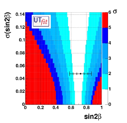
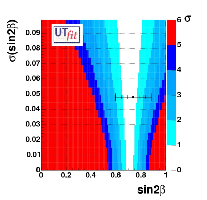
Figure 13: The compatibility (“pull”) between the direct and indirect determination of $\sin{2\beta}$ as a function of the value and error of $\sin{2\beta}$ measured from CP asymmetry in $J/\psi K^{0}$ decays. The indirect distribution of $\sin{2\beta}$ is computed without using the direct measurement (left plot) or using the measurement of $\sin{2\beta}$ from CP asymmetry in $J/\psi K^{0}$ decays (right plot). The compatibility regions from 1 to 6 $\sigma$ are also displayed.

¿From the left plot in Figure 13, it can be seen that, considering the actual precision of about 0.05 on the measured value of $\sin{2\beta}$, the 3$\sigma$ compatibility region is between [0.49-0.87]. Values outside this range would be, therefore, not compatible with the SM prediction at more than $3\sigma$ level. To get these values, however, the presently measured central value should shift by more than $4\sigma$.

The conclusion that can be derived from Figure 13 is the following: although the improvement of the error on sin2$\beta$ has an important impact on the accuracy of the UT parameter determination, it is very unlikely that in the near future we will be able to use this measurement to detect any failure of the SM, unless the other constraints entering the fit improve substantially or, of course, in case the central value of the direct measurement move away from the present one by several standard deviations.

The right plot in Figure 13 shows the compatibility of the direct and indirect distributions of $\sin{2\beta}$ as a function of the measured value and error of $\sin{2\beta}$. The difference with respect to the left plot is that, in this case, all the available constraints have been used to obtain the indirect distribution of $\sin{2\beta}$, including the direct measurement of $\sin{2\beta}$ from $J/\psi K^{0}$.

It was pointed out some time ago that the comparison of the time-dependent CP asymmetries in various $B$ decay modes could provide evidence of NP in B decay amplitudes [15]. Since $\sin{2\beta}$ is known from $J/\psi K^{0}$, a significant deviation of the time-dependent asymmetry parameters of penguin dominated channels $B^{0}\to\phi K^{0}$ and $B^{0}\to K^{0}\pi^{0}$ from their expected values would indicate the presence of NP.

These asymmetries have been recently measured at B-Factories [16] and are reported in Table 12.

Observable BaBar Belle Average $S_{\phi K^{0}_{S}}$ 0.47 $\pm$ 0.34${}^{+0.08}_{-0.06}$ -0.96 $\pm$ 0.50${}^{+0.09}_{-0.11}$ 0.02 $\pm$ 0.29 $C_{\phi K^{0}_{S}}$ 0.01 $\pm$ 0.33 $\pm$ 0.10 0.15 $\pm$ 0.29 $\pm$ 0.08 0.09 $\pm$ 023 $S_{K^{0}_{S}\pi^{0}}$ 0.48${}^{+0.38}_{-0.47}$ $\pm$ 0.11 - 0.48${}^{+0.38}_{-0.47}$ $\pm$ 0.11 $C_{K^{0}_{S}\pi^{0}}$ 0.40${}^{+0.27}_{-0.28}$ $\pm$ 0.10 - 0.40${}^{+0.27}_{-0.28}$ $\pm$ 0.10

Table 12: Experimental inputs for S and C in $B^{0}\to\phi K^{0}_{S}$ and $B^{0}\to K^{0}_{S}\pi^{0}$ decays [4].

In a naïve approach, one expects S $\sim\sin 2\beta$ and C $\sim$ 0, but the theoretical uncertainties related to hadronic physics can change this expectation. Starting from the value of sin2$\beta$ of the standard analysis, we used the Charming Penguins model [17] to take into account these hadronic uncertainties and quantify the sensitivity of future measurements with the compatibility plots shown in Figure 14. It has to be noted that, including these hadronic uncertainties, the theoretical predictions of $S$ and $C$ in Table 12 have a typical uncertainty of $\sim 0.09$ [18].

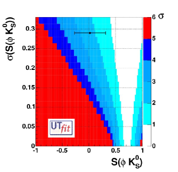
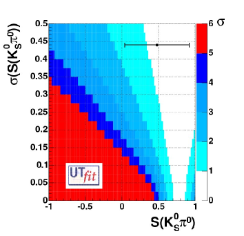
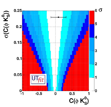
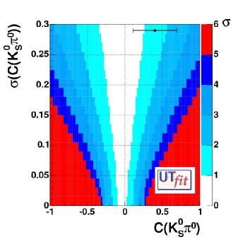
Figure 14: Compatibility plot for S (top) and C (bottom) for $\phi K^{0}_{S}$ (left) and $K^{0}_{S}\pi^{0}$ (right), using UTfit result and Charming Penguins model. Experimental measurements are superimposed.

5.3 Pull distribution for $\Delta m_{s}$

The plot in Figure 15 shows the compatibility of the indirect determination of $\Delta m_{s}$ with a future determination of the same quantity, obtained using or ignoring the experimental information coming from the present bound.

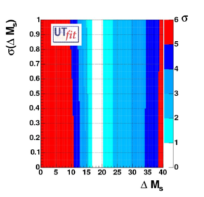
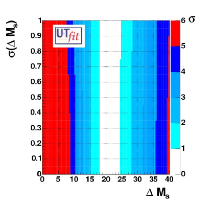
Figure 15: The compatibility of the direct and indirect determination of $\Delta m_{s}$, as a function of the value of $\Delta m_{s}$, using (left) or ignoring (right) the present experimental bound.

¿From the plot in Figure 15 it can be concluded that, once a measurement of $\Delta m_{s}$ with the expected accuracy of $\sim 1$ ps^-1 is available, a value of $\Delta m_{s}$ greater than $32$ ps^-1 would imply New Physics at $3~{}\sigma$ level.

5.4 Pull distribution for the angle $\gamma$

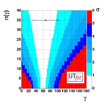
Figure 16: The compatibility of the direct and indirect determination of $\gamma$, as a function of the value and the error of $\gamma$, using the UT fit results.

The plot in Figure 16 shows the compatibility of the indirect determination of $\gamma$ with a future determination of the same angle obtained from B decays. It can be noted that even in case the angle $\gamma$ can be measured with a precision of 10^∘ from B decays, the predicted 3$\sigma$ region is still rather large, corresponding to the interval [25-100]^∘. Values beyond 100^∘ would clearly indicate physics beyond the Standard Model. The actual determination of the angle $\gamma$ is not yet precise enough to test the validity of the Standard Model as shown by the point with the error bar in Figure 16 and given in equation (6). Nevertheless, a direct determination of $\gamma$ is of crucial importance to test NP models [19].

6 Conclusions

Flavour physics in the quark sector has entered its mature age. Today the Unitarity Triangle parameters are known with good precision. A crucial test has been already done: the comparison between the Unitarity Triangle parameters, as determined with quantities sensitive to the sides of the triangle (semileptonic B decays and oscillations), and the measurements of CP violation in the kaon ($\epsilon_{K}$) and in the B (sin2$\beta$) sectors. The agreement is “unfortunately” excellent. The Standard Model is “Standardissimo”: it is also working in the flavour sector. This agreement is also due to the impressive improvements achieved on OPE, HQET and LQCD theories which have been used to extract the CKM parameters.

Many B decay Branching Fractions and relative CP asymmetries have been measured at B-Factories. The outstanding result is the determination of sin 2$\beta$ from B hadronic decays into charmonium-$K^{0}$ final states. On the other hand many other exclusive hadronic rare B decays have been measured and constitute a gold mine for weak and hadronic physics, allowing in principle to extract different combinations of the Unitarity Triangle angles.

Besides presenting an update of the standard UT analysis, we have shown in this paper that new measurements at B-Factories start to have an impact on the overall picture of the Unitarity Triangle determination. In the following years they will provide further tests of the Standard Model in the flavour sector to an accuracy up to the per cent level.

Finally, introducing the compatibility plots, we have studied the impact of future measurements on testing the SM and looking for New Physics.

7 Acknowledgements

We would like to warmly thank people which provide us the experimental and theoretical inputs which are an essential part of this work and helped us with useful suggestions for the correct use of the experimental information. We thank: A. Bevan, T. Browder, C. Campagnari, G. Cavoto, M. Danielson, R. Faccini, F. Ferroni, M. Legendre, O. Long, F. Martinez, L. Roos, A. Poulenkov, M. Rama, Y. Sakai, M.-H. Schune, W. Verkerke, M. Zito. We also thank P. Gambino and A. Soni for useful discussions. Finally, we thank M. Baldessari, C. Bulfon, and all the BaBar Rome group for help in the realization and for hosting the web site.

References

-
[1]
UTfit Collaboration : M. Bona, M.
Ciuchini, G. D’Agostini, E. Franco, V. Lubicz, G. Martinelli,
F.Parodi, M. Pierini, P. Roudeau, C.
Schiavi, L. Silvestrini, A. Stocchi.
http://www.utfit.org -
[2]
M. Ciuchini, E. Franco, V. Lubicz, F. Parodi, L.
Silvestrini and A. Stocchi, “Unitarity Triangle in the Standard
Model and sensitivity
to new physics” (hep-ph/0307195);
M. Ciuchini, G. D’Agostini, E. Franco, V. Lubicz, G. Martinelli, F. Parodi, P. Roudeau, A. Stocchi, “2000 CKM-Triangle Analysis A Critical Review with Updated Experimental Inputs and Theoretical Parameters”, JHEP 0107 (2001) 013. (hep-ph/0012308); A. J. Buras, F. Parodi, A. Stocchi, “The CKM Matrix and The Unitarity Triangle: another Look” JHEP 0301 (2003) 029 (hep-ph/0207101). - [3] M. Lusignoli, L. Maiani, G. Martinelli and L. Reina, Nucl. Phys. B 369, 139 (1992); A. Ali and D. London, arXiv:hep-ph/9405283; arXiv:hep-ph/9409399; Z. Phys. C 65, 431 (1995); S. Herrlich and U. Nierste, Phys. Rev. D 52, 6505 (1995); M. Ciuchini, E. Franco, G. Martinelli, L. Reina and L. Silvestrini, Z. Phys. C 68, 239 (1995); A. Ali and D. London, Nuovo Cim. 109A, 957 (1996); A. Ali, Acta Phys. Polon. B 27, 3529 (1996); A. J. Buras, arXiv:hep-ph/9711217; A. J. Buras and R. Fleischer, Adv. Ser. Direct. High Energy Phys. 15, 65 (1998); R. Barbieri, L. J. Hall, S. Raby and A. Romanino, Nucl. Phys. B 493, 3 (1997); A. Ali and B. Kayser, arXiv:hep-ph/9806230; P. Paganini, F. Parodi, P. Roudeau and A. Stocchi, Phys. Scripta 58, 556 (1998); F. Parodi, P. Roudeau and A. Stocchi, Nuovo Cim. A 112, 833 (1999); F. Caravaglios, F. Parodi, P. Roudeau and A. Stocchi, arXiv:hep-ph/0002171; S. Mele, Phys. Rev. D 59, 113011 (1999); A. Ali and D. London, Eur. Phys. J. C 9, 687 (1999); M. Ciuchini, E. Franco, L. Giusti, V. Lubicz and G. Martinelli, Nucl. Phys. B 573, 201 (2000); M. Bargiotti et al., La Rivista del Nuovo Cimento Vol. 23N3 (2000) 1; S. Plaszczynski and M. H. Schune, arXiv:hep-ph/9911280; S. Mele, in Proc. of the 5th International Symposium on Radiative Corrections (RADCOR 2000) ed. Howard E. Haber, arXiv:hep-ph/0103040; A. Hocker, H. Lacker, S. Laplace and F. Le Diberder, Eur. Phys. J. C 21 (2001) 225; M. Ciuchini, Nucl. Phys. Proc. Suppl. 109B (2002) 307; A. Hocker, H. Lacker, S. Laplace and F. Le Diberder, AIP Conf. Proc. 618 (2002) 27; F. Caravaglios, P. Roudeau and A. Stocchi, Nucl. Phys. B 633 (2002) 193; A. J. Buras, arXiv:hep-ph/0210291; G. P. Dubois-Felsmann, D. G. Hitlin, F. C. Porter and G. Eigen, arXiv:hep-ph/0308262; arXiv:hep-ex/0312062; A. Stocchi, arXiv:hep-ph/0405038; J. Charles et al. [CKMfitter Group Collaboration], arXiv:hep-ph/0406184.
- [4] HFAG: http://www.slac.stanford.edu/xorg/hfag/
- [5] “THE CKM MATRIX AND THE UNITARITY TRIANGLE”. Based on the First Workshop on “CKM Unitarity Triangle” held at CERN, 13-16 February 2002. Edited by: M. Battaglia, A. Buras, P. Gambino and A. Stocchi. To be published as CERN Yellow Book (hep-ph/0304132).
- [6] Proceedings of the Second Workshop on “CKM Unitarity Triangle” held in Durham, 5-9 April 2003. Edited by: P. Ball, P. Kluit, J. Flynn and A. Stocchi.
- [7] C. Dib, I. Dunietz, F. Gilman, Y. Nir, Phys. Rev. D41 (1990) 1522; G. Buchalla, A.J. Buras and M.E. Lautenbacher, Rev. Mod. Phys. 68 (1996) 1125; A. Ali and D. London, in Proceeding of “ECFA Workshop on the Physics of a Meson Factory”, Ed. R. Aleksan, A. Ali (1993); A. Ali and D. London, Nucl. Phys. 54A (1997) 297.
- [8] M. Gronau and D. London, Phys. Lett. B253, 483 (1991); M. Gronau and D. Wyler, Phys. Lett. B265, 172 (1991); I. Dunietz, Phys. Lett. B270, 75 (1991); I. Dunietz, Z. Phys. C56, 129 (1992); D. Atwood, G. Eilam, M. Gronau and A. Soni, Phys. Lett. B341, 372 (1995); D. Atwood, I. Dunietz and A. Soni, Phys. Rev. Lett. 78, 3257 (1997).
- [9] A. Giri, Yu. Grossman, A. Soffer and J. Zupan, Phys. Rev. D68, 054018 (2003).
- [10] A. Poluektov et al. [Belle Collaboration], arXiv:hep-ex/0406067.
- [11] M. Gronau and D. London, Phys. Rev. Lett. 65 (1990) 3381.
- [12] O. Long, M. Baak, R. N. Cahn and D. Kirkby, Phys. Rev. D 68 (2003) 034010 [arXiv:hep-ex/0303030].
- [13] B. Aubert et al. [BABAR Collaboration], arXiv:hep-ex/0309017. K. Abe et al. [BELLE Collaboration], arXiv:hep-ex/0308048.
- [14] B. Aubert et al. [BABAR Collaboration], Phys. Rev. Lett. 92 (2004) 251802 [arXiv:hep-ex/0310037].
- [15] Y. Grossman and M. P. Worah, Phys. Lett. B 395 (1997) 241 [arXiv:hep-ph/9612269]; M. Ciuchini, E. Franco, G. Martinelli, A. Masiero and L. Silvestrini, Phys. Rev. Lett. 79 (1997) 978 [arXiv:hep-ph/9704274]; Y. Grossman, G. Isidori and M. P. Worah, Phys. Rev. D 58 (1998) 057504 [arXiv:hep-ph/9708305].
- [16] B. Aubert et al. [BABAR Collaboration], arXiv:hep-ex/0403026. K. Abe et al. [Belle Collaboration], Phys. Rev. Lett. 91 (2003) 261602 [arXiv:hep-ex/0308035]. B. Aubert et al. [BABAR Collaboration], arXiv:hep-ex/0403001.
- [17] M. Ciuchini, E. Franco, G. Martinelli, M. Pierini and L. Silvestrini, Phys. Lett. B 515 (2001) 33 [arXiv:hep-ph/0104126].
- [18] M. Ciuchini, E. Franco, G. Martinelli, A. Masiero, M. Pierini and L. Silvestrini, arXiv:hep-ph/0407073.
- [19] M. Ciuchini, E. Franco, F. Parodi, V. Lubicz, L. Silvestrini and A. Stocchi, eConf C0304052 (2003) WG306 [arXiv:hep-ph/0307195].