Model-independent search for the Abelian $Z^{\prime}$ boson in the Bhabha process

Abstract

Model-independent observables to pick out the Abelian $Z^{\prime}$ signal in the Bhabha process are introduced at energies $\sqrt{s}\geq 200$ GeV. They measure separately the $Z^{\prime}$-induced vector and axial-vector four-fermion contact couplings. The analysis of the LEP2 data constrains the value of the $Z^{\prime}$-induced vector four-fermion coupling at the $2\sigma$ confidence level that corresponds to the Abelian $Z^{\prime}$ boson with the mass of order 1 TeV.

I Introduction

The LEP2 experiments have successfully confirmed the predictions of the Standard model (SM). At the same time, they inspire numerous estimations of possible new heavy particles beyond the SM. In particular, searching for “new physics” has already become an obligatory part of the reports on modern experiments in high energy physics. To describe possible signals of new physics beyond the SM the LEP2 collaborations apply both the model-dependent and the model-independent analysis of experimental data. The former approach means the comparison of experimental data with the predictions of some specific models which extend the SM at high energies. In this way a number of grand unified theories, the supersymmetry models were discussed and their parameters have been restricted. These model-dependent bounds are adduced in the reports EWWG .

In the model-independent approach one fits some low-energy parameters such as the four-fermion contact couplings. To establish a model-independent fit one has to take into consideration all possible coupling constants of a new heavy particle with the SM particles and introduce the observables which pick only one of these parameters. To find the expected signals the LEP collaborations have applied a “helicity model fit”. In this analysis an effective Lagrangian describing contact interactions of massless fermion states with one specific helicity (axial-axial (AA) model, vector-vector (VV) model, etc.) was introduced and the corresponding couplings have been restricted. This approach, giving a possibility to detect the signals of new physics, does not discern the specific state (its quantum numbers) responsible for them. This is because the particle interactions are described by a number of structures which contribute to different “helicity models”. Therefore a specific particle contributes to a number of the “models”.

In this regard, it seems resonable to develop an approach allowing to pick out in a model-independent way the parameters of new heavy particles with specified quantum numbers. In the previous papers PRD00 ; ZprTHDM ; YAF04 we established a model-independent search for manifestations of a heavy Abelian $Z^{\prime}$ boson beyond the SM. The key point of this analysis was the fact that for any theory beyond the SM which is renormalizable one (but unspecified in other respects) some relations between the unknown low energy $Z^{\prime}$ couplings with fermions hold PRD00 . In particular, they require an universal value of the $Z^{\prime}$ couplings to the axial-vector fermion currents. Taking into account these model-independent relations as well as the kinematics features of the processes $e^{+}e^{-}\to\mu^{+}\mu^{-},\tau^{+}\tau^{-}$, we introduced the unique sign-definite observable to select the signal of the virtual $Z^{\prime}$ state PRD00 . The value of the observable measures the $Z^{\prime}$-induced four-fermion coupling of the axial-vector currents. The analysis of the LEP2 data set on $e^{+}e^{-}\to\mu^{+}\mu^{-},\tau^{+}\tau^{-}$ processes has shown that the mean value of the observable is in an accordance with the signal although the accuracy is at the 1$\sigma$ confidence level (CL). Clearly, this could not be regarded as the actual observation of the particle.

As numerous estimates for various scattering processes showed the LEP2 data set is not too large to detect the signals of new physics at more then the $1\sigma$ CL (see, for instance, Refs. EWWG ; bourilkov ). Such an accuracy is insufficient for a real discovery. However, one may believe that the signals would appear more evidently if the statistics increases. One of the ways to ensure that within the existing data set is to follow the third of the described approaches and investigate other processes where the virtual states of the chosen new heavy particles contribute and can be identified. If again the observables to single out them are introduced and the data set is treated accordingly, one obtains an independent information about the states. Then, dependently on the results, one is able to conclude about the existence of the states and their characteristics by accounting for both of experiments that increases statistics.

These speculations served as a motivation for investigations carried out in the present paper in order to search for the Abelian $Z^{\prime}$ gauge boson in the Bhabha processes $e^{+}e^{-}\rightarrow e^{+}e^{-}(\gamma)$. We introduce new model-independent observables sensitive to the vector, $v_{f}$, and axial-vector, $a_{f}$, $Z^{\prime}$ couplings to the electron (positron) currents. They can be constructed from differential cross-sections at the LEP2 energies as well as at the energies of future electron-positron colliders ($\geq 500$ GeV). As an application, we analyse the existing in the literature LEP2 data on the Bhabha process and derive limits on fitted parameters. The comparison with the results obtained already for the $e^{+}e^{-}\rightarrow\mu^{+}\mu^{-},\tau^{+}\tau^{-}$ processes is done. We also confront our results with other analysises for Bhabha process. The paper is organized as follows. In sect. II we introduce the effective Lagrangian describing the $Z^{\prime}$-boson interaction with fermions at low energies as well as other necessary information on the model-independent search for this state at low energies. In sect. III we investigate the differential cross-sections with taking into consideration the relations between $a_{f}$ and $v_{f}$ parameters peculiar for the Abelian $Z^{\prime}$ that gives a possibility to identify this virtual state. In sects. IV, V the observables to pick out $v^{2}_{f}$ and $a^{2}_{f}$ are introduced. The last two sections are devoted to the analysis of the LEP2 data and discussion.

II The Abelian $Z^{\prime}$ couplings to the SM particles

The $Z^{\prime}$-boson can be introduced in a phenomenological way by specifying its effective low-energy couplings to the known SM particles leike . Considering the $Z^{\prime}$ effects at energies much below the $Z^{\prime}$ mass, it is enough to parametrize the tree-level $Z^{\prime}$ interactions of renormalizable types, only. Such a possibility is provided by the decoupling theorem decoupling from which, in particular, it follows that the non-renormalizable $Z^{\prime}$ interactions are produced by loops at higher energies and suppressed by powers of the inverse $Z^{\prime}$ mass. The SM gauge group $SU(2)_{L}\times U(1)_{Y}$ is usually considered as a subgroup of an underlying theory gauge group, so the vector-boson interactions of types $Z^{\prime}W^{+}W^{-}$, $Z^{\prime}ZZ$, … are absent at a tree level arzt . Thus, to investigate the $Z^{\prime}$ effects in the leptonic processes at the energies of LEP experiments ($\sqrt{s}\sim 200$ GeV) or future electron-positron colliders ($\sqrt{s}\geq 500$ GeV) we use the Lagrangian:

$${\cal L} = \left|\left(D^{{\rm ew,}\phi}_{\mu}-\frac{i\tilde{g}}{2}\tilde{Y}(\phi)\tilde{B}_{\mu}\right)\phi\right|^{2}+$$ (1)

$$i\sum\limits_{f=f_{L},f_{R}}\bar{f}{\gamma^{\mu}}\left(D^{{\rm ew,}f}_{\mu}-\frac{i\tilde{g}}{2}\tilde{Y}(f)\tilde{B}_{\mu}\right)f,$$

where $\phi$ is the SM scalar doublet, $\tilde{B}_{\mu}$ denotes the $Z^{\prime}$ field before the spontaneous breaking of the electroweak symmetry, and summation over the all SM left-handed fermion doublets, $f_{L}=\{(f_{u})_{L},(f_{d})_{L}\}$, and the right-handed singlets, $f_{R}=(f_{u})_{R},(f_{d})_{R}$, is assumed. The notation $\tilde{g}$ stands for the charge corresponding to the $Z^{\prime}$ gauge group, $D^{{\rm ew,}\phi}_{\mu}$ and $D^{{\rm ew,}f}_{\mu}$ are the electroweak covariant derivatives. Diagonal $2\times 2$ matrices $\tilde{Y}(\phi)={\rm diag}(\tilde{Y}_{\phi,1},\tilde{Y}_{\phi,2})$, $\tilde{Y}(f_{L})={\rm diag}(\tilde{Y}_{L,f_{u}},\tilde{Y}_{L,f_{d}})$ and numbers $\tilde{Y}(f_{R})=\tilde{Y}_{R,f}$ mean the unknown $Z^{\prime}$ generators characterizing the model beyond the SM.

The Lagrangian (1) generally leads to the $Z$–$Z^{\prime}$ mixing of order $m^{2}_{Z}/m^{2}_{Z^{\prime}}$ which is proportional to $\tilde{Y}_{\phi,2}$ and originated from the diagonalization of the neutral vector boson mass matrix. This mixing contributes to the scattering amplitudes and plays an important role at the LEP2 energies NPB .

The low energy $Z^{\prime}$ couplings to a fermion $f$ are parameterized by two numbers $\tilde{Y}_{L,f}$ and $\tilde{Y}_{R,f}$. Alternatively, the couplings to the axial-vector and vector fermion currents, $a^{l}_{Z^{\prime}}\equiv(\tilde{Y}_{R,l}-\tilde{Y}_{L,l})/2$ and $v^{l}_{Z^{\prime}}\equiv(\tilde{Y}_{L,l}+\tilde{Y}_{R,l})/2$, are often used. Their specific values are determined by the unknown model beyond the SM. Assuming an arbitrary underlying theory one usually supposes the parameters $a_{f}$ and $v_{f}$ are to be independent numbers. However, as it was proved in Ref. ZprTHDM , for any renormalizable theory beyond the SM these parameters content some relations which follow from the renorlalization group equations and the decoupling theorem. In case of the $Z^{\prime}$ boson this is reflected in correlations between $a_{f}$ and $v_{f}$. These correlations are model-independent in sense that they do not depend on an particular underlying model. The detailed discussion of these issues and the derivation of the RG relations are presented in Ref. ZprTHDM . Therein, in particular, it is shown that the low energy Abelian $Z^{\prime}$ couplings are constrained by the relations

$$v_{f}-a_{f}=v_{f^{\star}}-a_{f^{\star}},\quad\tilde{Y}_{\phi,1}=\tilde{Y}_{\phi,2}\equiv\tilde{Y}_{\phi},$$

$$a_{f}=T_{3,f}\tilde{Y}_{\phi},$$ (2)

where $T^{3}_{f}$ is the third component of the fermion weak isospin, and $f^{\star}$ means the isopartner of $f$ (namely, $l^{\star}=\nu_{l},\nu^{\star}_{l}=l,\ldots$).

The correlations (II) result in important properties of the Abelian $Z^{\prime}$ couplings. They ensure, in particular, the invariance of the Yukawa terms with respect to the effective low-energy $\tilde{U}(1)$ subgroup corresponding to the Abelian $Z^{\prime}$ boson. As it follows from the relations, the couplings of the Abelian $Z^{\prime}$ to the axial-vector fermion currents have the universal absolute value proportional to the $Z^{\prime}$ coupling to the scalar doublet. So, we will use the short notation $a=a_{l}=-\tilde{Y}_{\phi}/2$.

The relations (II) allow to reduce the number of independent parameters of new physics. The leading-order differential cross-section of the Bhabha process depends on five different combinations of $Z^{\prime}$ couplings: $a_{e}^{2}$, $v_{e}^{2}$, $a_{e}v_{e}$, $a_{e}\tilde{Y}_{\phi}$, and $v_{e}\tilde{Y}_{\phi}$. Taking into account these correlations reduce them to three actual parameters $a_{e}^{2}$, $v_{e}^{2}$, and $a_{e}v_{e}$. As it will be shown, the factors at $a_{e}^{2}$ and $v_{e}^{2}$ are dominant. Therefore, with a high accuracy the differential cross-section is a two-parametric function.

In Refs. PRD00 ; YAF04 we showed for the processes $e^{+}e^{-}\to\mu^{+}\mu^{-},\tau^{+}\tau^{-}$, that the many-parametric differential cross section can be integrated over a special range of the scattering angles in order to select only one of the unknown parameters. It seems resonable to apply similar approach in order to measure separately the couplings $a_{e}^{2}$ and $v_{e}^{2}$ by using the differential cross-section of the Bhabha process. Such kind of observables can be fitted by means of treating of modern experimental data that provides the bounds on the low energy vector and the axial-vector $Z^{\prime}$ couplings to electron. Due to the mentioned above universality of the axial-vector coupling $a^{2}$ it is possible to compare the estimates derived in different independent processes.

III Cross-section

Figure 1: Factors at $\bar{v}^{2}$, $\bar{a}^{2}$, and $\bar{a}\bar{v}$ in the differential cross-section $\Delta\,d\sigma/dz$ for $\sqrt{s}=200$ and 500 GeV.

The contributions to the cross-section of the process $e^{+}e^{-}\to e^{+}e^{-}(\gamma)$ in the so-called improved Born approximation are described by the tree-level plus one-loop diagrams with the neutral vector boson exchange in the $s$ and $t$ channels. The virtual states of the Abelian $Z^{\prime}$ boson cause the differential cross-section to differ from its SM value:

$$\Delta\,\frac{d\sigma}{dz} = \frac{d\sigma}{dz}-\frac{d\sigma^{\rm SM}}{dz}={\cal F}_{v}(\sqrt{s},z)\bar{v}^{2}+$$ (3)

$$+{\cal F}_{a}(\sqrt{s},z)\bar{a}^{2}+{\cal F}_{av}(\sqrt{s},z)\bar{a}\bar{v}+\ldots,$$

where $z=\cos\theta$, $\theta$ – scattering angle and we introduced the dimensionless couplings

$$\bar{a}=a_{e}\sqrt{\frac{\tilde{g}^{2}}{4\pi}\frac{m_{Z}^{2}}{m_{Z^{\prime}}^{2}}},\quad\bar{v}=v_{e}\sqrt{\frac{\tilde{g}^{2}}{4\pi}\frac{m_{Z}^{2}}{m_{Z^{\prime}}^{2}}}.$$ (4)

Due to the correlations (II) the cross-section contains only three different combinations of the $Z^{\prime}$ couplings $a_{e}^{2}$, $v_{e}^{2}$, and $a_{e}v_{e}$. The factors ${\cal F}(\sqrt{s},z)$ standing at them depend on the SM couplings and particle masses. For the purposes of the present investigation the values of running couplings were taken at $\sqrt{s}\sim 200$ GeV. The dots in Eq. (3) denote the neglected contributions of the box diagrams and diagrams describing emission of soft photons in the initial and final states. These terms can be estimated to be of the order of a few percents of the total and are inessential for what follows. The explicit expressions for the tree-level functions ${\cal F}(\sqrt{s},z)$ are adduced in the Appendix. Their plots are shown in Fig. 1. As it is seen, each factor is infinitely increasing at $z\to 1$. This is caused by the photon exchange in the $t$-channel.

Figure 2: The function $f_{\mathrm{mix}}(\sqrt{s},z)$ for the center-of-mass energy $\sqrt{s}=200$ GeV (solid curve) and $\sqrt{s}=500$ GeV (dashed curve).

Figure 3: The ratio ${\cal F}_{a}(z)/{\cal F}_{v}(z)$ of the factors at $\bar{a}^{2}$ and $\bar{v}^{2}$ in the differential cross-section $\Delta\,d\sigma/dz$ at various hypothetic values of $\tilde{Y}_{\phi}/a_{e}$. The plots correspond to $\tilde{Y}_{\phi}/a_{e}=-4$ (curve a), $-2$ (curve b, the Abelian $Z^{\prime}$), 0 (curve c), and 2 (curve d). The center-of-mass energy is $\sqrt{s}=200$ GeV.

As it was mentioned above, the $Z$–$Z^{\prime}$ mixing is expressed in terms of the axial-vector coupling. So, it influences the factors ${\cal F}_{a}(\sqrt{s},z)$ and ${\cal F}_{av}(\sqrt{s},z)$. Without taking into consideration the correlations (II) the contribution of the mixing to the cross-section has the form

$$\left.\Delta\,\frac{d\sigma}{dz}\right|_{\mathrm{mix}}=-\frac{\alpha_{\mathrm{em}}}{144s(1-z)}\frac{\tilde{g}^{2}m_{Z}^{2}}{m_{Z^{\prime}}^{2}}\tilde{Y}_{\phi}\,a_{e}\,f_{\mathrm{mix}}(\sqrt{s},z).$$ (5)

The dimensionless function $f_{\mathrm{mix}}(\sqrt{s},z)$ is adduced in the Appendix. For definiteness we show its angular dependence at the center-of-mass energies 200 and 500 GeV in Fig. 2. The factor $f_{\mathrm{mix}}(\sqrt{s},z)$ is a non-zero quantity which is almost an energy-independent constant at $z<0.5$. The contribution of the mixing (5) decreases when the center-of-mass energy grows. At LEP2 energies the account of the $Z$–$Z^{\prime}$ mixing plays an important role. Actually, because of the correlation (II) the mixing terms essentially influence the factors at axial-vector couplings in the cross-section. The Abelian $Z^{\prime}$ signal is charachterized by the value $\tilde{Y}_{\phi}=-2a_{e}$. The function ${\cal F}_{a}(\sqrt{s},z)$ corresponding to this number is close to zero almost in all $z$ interval and qualitatively distinguishable among the factors for other hypothetic values of $\tilde{Y}_{\phi}/a_{e}$ (see Fig. 3). Hence, it is impossible to search for the signals of the Abelian $Z^{\prime}$ boson omitting the $Z^{\prime}$–scalar coupling $\tilde{Y}_{\phi}$. Setting $\tilde{Y}_{\phi}$ to zero, one obtains ${\cal F}_{a}(\sqrt{s},z)$ which behavior does not reflect in general the virtual state under consideration.

In order to study the deviations from the SM cross-section inspired by the heavy virtual state of the Abelian $Z^{\prime}$ boson, we introduce the functions which are finite at all values of the scattering angle. They are determined by means of dividing the differential cross-section by some known monotonic function.

The factor ${\cal F}_{v}(z)$ is positive monotonic function of $z$ plotted in Fig. 4 for the center-of-mass energies $\sqrt{s}=200$ and 500 GeV. For intermediate energies the curves are in between these very close located curves (in the chosen energy scale). This type of behavior is typical for all other functions. So, in what follows, as illustration, we shall present our results for these two energies.

Figure 4: Factor ${\cal F}_{v}(z)$ at the vector-vector four-fermion coupling $\bar{v}^{2}$ in the deviation of the differential cross-section of the Bhabha process from the SM value, $\Delta\,d\sigma/dz$, for $\sqrt{s}=200$ GeV (solid) and $500$ GeV (dashed).

Such a property allows one to choose ${\cal F}_{v}(z)$ as a normalization factor for the differential cross section. Then the normalized differential cross-section reads

$$\frac{d\tilde{\sigma}}{dz} = {\cal F}_{v}^{-1}(\sqrt{s},z)\Delta\,\frac{d\sigma}{dz}=$$ (6)

$$\bar{v}^{2}+F_{a}(\sqrt{s},z)\bar{a}^{2}+F_{av}(\sqrt{s},z)\bar{a}\bar{v}+\ldots,$$

and the normalized factors are shown in Fig 5.

Figure 5: Factors $F_{a}$ (solid) and $F_{av}$ (dashed) in the normalized differential cross-section $\Delta\,d\tilde{\sigma}/dz$ for $\sqrt{s}=200$ and 500 GeV.

Now these factors are finite at $z\to 1$. Each of them in a special way influences the differential cross-section.

1. The factor at $\bar{v}^{2}$ is just the unity. Hence, the four-fermion contact coupling between vector currents, $\bar{v}^{2}$, determines the level of the deviation from the SM value.

2. The factor at $\bar{a}^{2}$ depends on the scattering angle in a non-trivial way. It allows to recognize the Abelian $Z^{\prime}$ boson, if the experimental accuracy is sufficient.

3. The factor at $\bar{a}\bar{v}$ results in small corrections.

Thus, effectively, the obtained normalized differential cross-section is a two-parametric function. In the next sections we introduce the observables to fit separately each of these parameters.

IV Observables to pick out $\bar{v}^{2}$

To recognize the signal of the Abelian $Z^{\prime}$ boson by analyzing the Bhabha process the differential cross-section deviation from the SM predictions should be measured with a good accuracy. At present, no such deviations have been detected at more than the 1$\sigma$ CL. In this situation it is resonable to introduce integrated observables allowing to pick out $Z^{\prime}$ signals by using the most effective treating of available data. The observables should be sensitive to the separate $Z^{\prime}$ couplings. This admits of search for the $Z^{\prime}$ signals in different processes as well as to perform global fits.

The deviation of the normalized differential cross-section (6) is (effectively) the function of two parameters, $\bar{a}^{2}$ and $\bar{v}^{2}$. We are going to introduce the integrated observables which determine separately the four-fermion couplings $\bar{a}^{2}$ and $\bar{v}^{2}$.

Let us first proceed with the observable for $\bar{v}^{2}$. After normalization the factor at the vector-vector four-fermion coupling becomes the unity. Whereas the factor at $\bar{a}^{2}$ is a sign-varying function of the cosine of the scattering angle. As it follows from Fig. 3, for the center-of-mass energy 200 GeV it is small over the backward scattering angles. So, to measure the value of $\bar{v}^{2}$ the normalized differential cross-section has to be integrated over the backward angles. For the center-of-mass energy 500 GeV the factor at $\bar{a}^{2}$ is already a non-vanishing quantity for the backward scattering angles. The curves corresponding to intermediate energies are distributed in between two these curves. Since they are sign-varying ones at each energy point some interval of $z$ can be chosen to make the integral to be zero. Thus, to measure the $Z^{\prime}$ coupling to the electron vector current $\bar{v}^{2}$ we introduce the integrated cross-section (6)

$$\sigma_{V}=\int_{z_{0}}^{z_{0}+\Delta z}(d\tilde{\sigma}/dz)dz,$$ (7)

where at each energy the most effective interval $[z_{0},z_{0}+\Delta z]$ is determined by the following requirements:

1. The relative contribution of the coupling $\bar{v}^{2}$ is maximal. Equivalently, the contribution of the factor at $\bar{a}^{2}$ is suppressed.

2. The length $\Delta z$ of the interval is maximal. This condition ensures that the largest number of bins is taken into consideration.

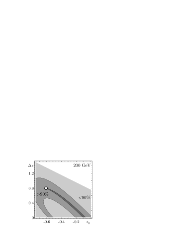
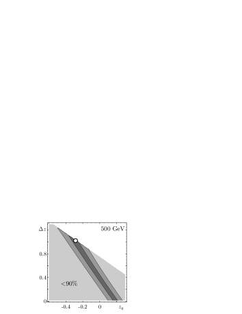
Figure 6: Relative contribution of the factor at $\bar{v}^{2}$ as the function of the left boundary of the angle interval, $z_{0}$, and the interval length, $\Delta z$, at the center-of-mass energy 200 and 500 GeV. The shaded areas correspond to the contributions $>95\%$ (dark), from 90% to 95% (midtone), and $<90\%$ (light).

The relative contribution of the factor at $\bar{v}^{2}$ is defined as

$$\kappa_{V}=\frac{\Delta z}{\Delta z+\left|\int_{z_{0}}^{z_{0}+\Delta z}F_{a}\,dz\right|+\left|\int_{z_{0}}^{z_{0}+\Delta z}F_{av}\,dz\right|}$$ (8)

and shown in Fig. 6 as the function of the left boundary of the angle interval, $z_{0}$, and the interval length, $\Delta z$. In each plot the dark area corresponds to the observables which values are determined by the vector-vector coupling $\bar{v}^{2}$ with the accuracy $>95\%$. The area reflects the correlation of the width of the integration interval $\Delta z$ with the choice of the initial $z_{0}$ following from the mentioned requirements. Within this area we choose the observable which includes the largest number of bins (largest $\Delta z$). The corresponding values of $z_{0}$ and $\Delta z$ are marked by the white dot on the plots in Fig. 6. As the carried out analysis showed, the point $z_{0}$ is shifted to the right with increase in energy whereas $\Delta z$ remains approximately the same.

From the plots it follows that the most efficient intervals are

$$-0.6<z<0.2,\quad\sqrt{s}=200\mbox{ GeV},$$

$$-0.3<z<0.7,\quad\sqrt{s}=500\mbox{ GeV}.$$ (9)

Therefore the observable (7) allows to measure the $Z^{\prime}$ coupling to the electron vector current $\bar{v}^{2}$ with the efficiency $>95\%$.

V Observables to pick out $\bar{a}^{2}$

In order to pick the axial-vector coupling $\bar{a}^{2}$ one needs to eliminate the dominant contribution coming from $\bar{v}^{2}$. Since the factor at $\bar{v}^{2}$ in the $d\tilde{\sigma}/dz$ equals unity, this can be done by summing up equal number of bins with positive and negative weights. In particular, the forward-backward normalized differential cross-section appears to be sensitive mainly to $\bar{a}^{2}$,

$$\tilde{\sigma}_{\rm FB} = \int\nolimits_{0}^{z_{\rm max}}dz\,\frac{d\tilde{\sigma}}{dz}-\int\nolimits_{-z_{\rm max}}^{0}dz\,\frac{d\tilde{\sigma}}{dz}$$ (10)

$$= \tilde{F}_{a,\rm FB}\bar{a}^{2}+\tilde{F}_{av,\rm FB}\bar{a}\bar{v}.$$

The value $z_{\rm max}$ is determined by the number of bins included and, in fact, depends on the data set considered. The LEP2 experiment accepted $e^{+}e^{-}$ events with $|z|<0.72$. In what follows we take $z=0.7$ for definiteness.

The efficiency of the observable is determined as:

$$\kappa=\frac{|\tilde{F}_{a,\rm FB}|}{|\tilde{F}_{a,\rm FB}|+|\tilde{F}_{av,\rm FB}|}.$$ (11)

It can be estimated as $\kappa=0.9028$ for the center-of-mass energy 200 GeV and $\kappa=0.9587$ for 500 GeV. To obtain this value we took typical $z_{\mathrm{max}}=0.7$. Thus, the observable

$$\tilde{\sigma}_{\rm FB}=0.224\bar{a}^{2}-0.024\bar{a}\bar{v},\quad\sqrt{s}=200\mbox{ GeV},$$

$$\tilde{\sigma}_{\rm FB}=0.472\bar{a}^{2}-0.020\bar{a}\bar{v},\quad\sqrt{s}=500\mbox{ GeV}$$ (12)

is mainly sensitive to the $Z^{\prime}$ coupling to the axial-vector current $\bar{a}^{2}$.

Consider a usual situation when experiment is not able to recognize the angular dependence of the differential cross-section deviation from its SM value with the proper accuracy because of loss of statistics. Nevertheless, a unique signal of the Abelian $Z^{\prime}$ boson can be determined. For this purpose the observables $\int_{z_{0}}^{z_{0}+\Delta z}(d\tilde{\sigma}/dz)dz$ and $\tilde{\sigma}_{\rm FB}$ must be measured. Actually, they are derived from the normalized differential cross-section. If the deviation from the SM is inspired by the Abelian $Z^{\prime}$ boson both the observables are to be positive quantities simultaneously. This feature serves as the distinguishable signal of the Abelian $Z^{\prime}$ virtual state in the Bhabha process for the LEP2 energies as well as for the energies of future electron-positron colliders ($\geq 500$ GeV). The observables fix the unknown low energy vector and axial-vector $Z^{\prime}$ couplings to the electron current. Their values have to be correlated with the bounds on $\bar{a}^{2}$ and $\bar{v}^{2}$ derived by means of independent fits for other scattering processes.

VI LEP II data analysis

Let us apply the introduced observables to analysis the experimental data on differential cross-sections of the Bhabha scattering. The LEP2 experiments have measured, in particular, the differential cross-section of this process at a number of energy points. Both the final and preliminary data are available in the literature LEPdata . These data provide an opportunity to estimate possible Abelian $Z^{\prime}$ virtual states.

In the present paper we take into consideration the differential cross-sections measured by the L3 Collaboration at 183-189 GeV, by the OPAL Collaboration at 189-207 GeV, as well as the cross-sections obtained by the DELPHI Collaboration at energies 189-207 GeV.

First, we estimate the value of the vector coupling $\bar{v}^{2}$ by using the observable (7). At the LEP2 energies the appropriate interval of the angular integration of the normalized differential cross-section is $-0.6<z<0.2$. The results are shown in Table 1 as ‘Fit 1’. The L3 and OPAL Collaborations demonstrate positive values of $\bar{v}^{2}$ at the $1\sigma$ CL, whereas the DELPHI Collaboration shows the $2\sigma$ positive deviation. To constrain the value of the $Z^{\prime}$ mass by the derived bounds on the four-fermion coupling $\bar{v}^{2}$ some value of $\tilde{g}$ should be fixed. Let us assume that the coupling $\tilde{g}$ is of order of SM gauge couplings, $\tilde{g}^{2}/(4\pi)\simeq 0.01-0.03$. Then the combined value of $\bar{v}^{2}$ corresponds to $m_{Z^{\prime}}=0.7-1.2$ TeV. It is interesting to note that the mean values of $\bar{v}^{2}$ are a little larger than those obtained for $\bar{a}^{2}$ for $e^{+}e^{-}\to\mu^{+}\mu^{-},\tau^{+}\tau^{-}$ processes YAF04 .

Table 1: Fits of the LEP2 data on the Bhabha process. Fit 1 represents the value of $\bar{v}^{2}$ derived with the observable $\sigma_{V}$ integrated in the angular interval $z\in(-0.6,0.2)$. In Fit 2 the axial-vector coupling $\bar{a}^{2}$ is fitted by the analysis of the observable $\tilde{\sigma}_{\mathrm{FB}}$. In Fit 3 the value of $\bar{a}^{2}=3.6\times 10^{-5}$ from the analysis of the $e^{+}e^{-}\to\mu^{+}\mu^{-}$ scattering process is taken, and the value of vector coupling $\bar{v}^{2}$ is found by fitting the total cross-section ($|z|<0.72$).

$\sqrt{s}$, GeV	$\bar{v}^{2}$, Fit 1	$\bar{a}^{2}$, Fit 2	$\bar{v}^{2}$, Fit 3
	$\times 10^{-4}$
DELPHI
189	$1.0\pm 2.8$	$-23\pm 16$	$0.9\pm 2.0$
192	$3.1\pm 6.5$	$4\pm 34$	$2.5\pm 4.4$
196	$5.1\pm 3.9$	$1\pm 20$	$5.0\pm 2.6$
200	$6.1\pm 3.7$	$-33\pm 20$	$3.0\pm 2.4$
202	$-1.6\pm 4.6$	$6\pm 25$	$0.8\pm 3.2$
205	$2.7\pm 3.4$	$-27\pm 19$	$0.8\pm 2.3$
207	$1.4\pm 2.9$	$-1\pm 15$	$-1.6\pm 1.9$
Combined	$2.39\pm 1.35$	$-12\pm 7$	$1.2\pm 0.9$
OPAL
189	$-2.8\pm 2.2$	$1\pm 12$	$0.2\pm 1.5$
192	$-2.4\pm 6.4$	$20\pm 34$	$1.6\pm 4.2$
196	$0.3\pm 3.1$	$1\pm 15$	$-0.1\pm 2.0$
200	$3.4\pm 3.1$	$-1\pm 16$	$2.9\pm 2.1$
202	$9.1\pm 5.6$	$-9\pm 27$	$3.5\pm 3.4$
205	$7.2\pm 3.1$	$-11\pm 16$	$3.9\pm 2.1$
207	$1.5\pm 2.3$	$-4\pm 13$	$1.7\pm 1.6$
Combined	$1.33\pm 1.14$	$-2\pm 6$	$1.6\pm 0.8$
L3
183	$3.7\pm 5.8$	$-36\pm 35$	$3.8\pm 5.0$
189	$1.9\pm 3.2$	$7\pm 18$	$-1.6\pm 2.6$
Combined	$2.36\pm 2.82$	$-2\pm 16$	$-0.4\pm 2.3$
COMBINED
	$1.82\pm 0.83$	$-6\pm 4$	$1.3\pm 0.6$

The second fit (‘Fit 2’) estimates the observable (V) related to the value of $\bar{a}^{2}$. Since in the Bhabha process the effects of the axial-vector coupling are suppressed with respect to those of the vector coupling, we expect much larger experimental uncertainties for $\bar{a}^{2}$. Indeed, the LEP2 data lead to the significant errors for $\bar{a}^{2}$ of order $10^{-3}-10^{-4}$ (See Table 1). The mean values are negative numbers which are too large to be interpreted as a manifestation of some heavy virtual state beyond the energy scale of the SM.

Finally, we performed also the fit of $\bar{v}^{2}$, assuming the value of the $Z^{\prime}$-induced axial-vector coupling from $e^{+}e^{-}\to\mu^{+}\mu^{-}$ process YAF04 . In this case, putting $\bar{a}^{2}=0.000037$ and computing the total cross-section ($|z|<0.72$), we obtain the observable which depends on one parameter $\bar{v}^{2}$, only. This parameter can be easily fitted. As it follows from Table 1, the results are close to those based on the observable (7) for the vector coupling.

Thus, the LEP2 data constrain the value of $\bar{v}^{2}$ at the $2\sigma$ CL which could correspond to the Abelian $Z^{\prime}$ boson with the mass of the order 1 TeV. In contrast, the value of $\bar{a}^{2}$ is a large negative number with a significant experimental uncertainty. This can not be interpreted as a manifestation of some heavy virtual state beyond the energy scale of the SM.

VII Conclusion

In the present paper we have introduced new observables for model-independent searches for the heavy Abelian $Z^{\prime}$ boson in the Bhabha process at the energies of the LEP and future linear electron-positron colliders. They are based on the specific correlations (II) existing at low energies between the vector and the axial-vector $Z^{\prime}$ couplings to fermions and therefore uniquely identify this virtual state. If, for instance, one does not take into consideration these relations, no estimation of the $v^{2}_{f}$ could be derived at all.

It is interesting to compare the results on the $Z^{\prime}$ search in the Bhabha processes with that of the processes $e^{+}e^{-}\to\mu^{+}\mu^{-},\tau^{+}\tau^{-}$ investigated already in Ref. YAF04 . Cross-sections for those processes involve quadratic combinations of electron couplings $a_{e}$, $v_{e}$ and muon (tau) couplings $a_{\mu}$, $v_{\mu}$ ($a_{\tau}$, $v_{\tau}$). Due to Eq. (II) the axial-vector coupling is universal, $a_{e}=a_{\mu}=a_{\tau}=a_{l}$. Therefore, there is the sign-definite term $a^{2}_{l}$ in the cross-section. A more simple kinematics of the processes $e^{+}e^{-}\to\mu^{+}\mu^{-},\tau^{+}\tau^{-}$ allows to introduce a one-parametric observable which is directly related to the coupling $a_{l}^{2}$. Just the sign of the observable serves as the signal of the Abelian $Z^{\prime}$ in this case. The following estimate has been derived:

$$\mu^{+}\mu^{-}: \bar{a}^{2}_{l}=(3.66\pm 4.89)\times 10^{-5},$$

$$\tau^{+}\tau^{-}: \bar{a}^{2}_{l}=(-2.66\pm 6.43)\times 10^{-5}.$$ (13)

The dimensionless coupling $\bar{a}_{l}$ is related to $a_{l}$ by means of Eq. (4) and actually identical to the parameter $\bar{a}$ admitted in the present paper. The more precise $\mu^{+}\mu^{-}$ data demonstrate the $1\sigma$ deviation whereas the $\tau^{+}\tau^{-}$ data do not specify the sign of the observable. As the value of $v^{2}_{f}$ is concerned, it remained completely unrestricted in that case because of the kinematics specifics. Thus, the results derived in the present paper from the analysis of the Bhabha process are complementary. We see also that the accuracy of the result is of $2\sigma$ CL vs. $1\sigma$ for $e^{+}e^{-}\rightarrow l^{+}l^{-}$.

There is a simple relation of the parameters $\bar{a}$, $\bar{v}$ used in the present paper to the four-fermion couplings $\epsilon_{AA}$, $\epsilon_{AV}$, and $\epsilon_{VV}$ admitted in the reports of the Electroweak Working Group EWWG . They are just normalized by different factors and related as $\epsilon_{AA}=-\bar{a}^{2}m^{-2}_{Z}/4$, $\epsilon_{AV}=-\bar{a}\bar{v}m^{-2}_{Z}/4$, and $\epsilon_{VV}=-\bar{v}^{2}m^{-2}_{Z}/4$. The description of the Abelian $Z^{\prime}$ virtual state in the Bhabha process requires both $\epsilon_{VV}$ and $\epsilon_{AA}$. None of these couplings should be set to zero in searching for $Z^{\prime}$ signals. The separate constraints on $\epsilon_{VV}$ or $\epsilon_{AA}$ could be performed by means of observables $\sigma_{V}$ and $\tilde{\sigma}_{\rm FB}$.

Let us confront our results with that in Ref. bourilkov where the ‘helicity model fit’ was applied for the total cross sections of the Bhabha process. The most interesting result of that analysis is the observation that for the AA-model the $2\sigma$ deviation from the SM has been derived. For other ‘models’ no distinguishable deviations were observed. Since our analysis is based on the properties of differential cross sections, no direct comparisons can be done. We just mention that in the paper YAF04 we showed that the AA-helicity model is mainly responsible for the signal of the Abelian $Z^{\prime}$ gauge boson. So, one may speculate that this fact found its implementation in the significant $2\sigma$ deviations.

As a general conclusion we would like to stress that the observables to search for the Abelian $Z^{\prime}$ signal in Bhabha process can be introduced at the LEP2 energies ($\sqrt{s}\simeq 200$ GeV) as well as at the energies of future electron-positron colliders ($\sqrt{s}\geq 500$ GeV). They are determined by normalized differential cross-section and measure two sign-definite $Z^{\prime}$ couplings, $v^{2}$ and $a^{2}$. The positive signs of the observables are the characteristic feature of the Abelian $Z^{\prime}$ virtual state. The corresponding values of $Z^{\prime}$ couplings could be compared with those obtained in other independent scattering processes.

In the Bhabha process the Abelian $Z^{\prime}$ effects are dominated by the vector coupling $v^{2}$. This process provides mainly constraints on the $Z^{\prime}$-induced vector-vector four-fermion coupling. Therefore it gives complementary information to the constraints on the axial four-fermion coupling $a^{2}$ based on the analysis of $e^{+}e^{-}\to\mu^{+}\mu^{-},\tau^{+}\tau^{-}$. From the carried out investigations we conclude that the $Z^{\prime}$ boson is expected to have the mass of the order $1-1.2$ TeV and has a good chance to be discovered at colliders of next generation.

Appendix

Below we adduce explicitly the factors ${\cal F}_{v}$, ${\cal F}_{a}$, ${\cal F}_{av}$ at the $Z^{\prime}$-induced couplings $\bar{v}^{2}$, $\bar{a}^{2}$ and $\bar{a}\bar{v}$ in the differential cross-section $\Delta\,d\sigma/dz$ (Eq. (3)). These factors are plotted in Fig. 1 at the so-called imroved-Born level. The complete expressions for ${\cal F}_{v}$, ${\cal F}_{a}$, and ${\cal F}_{av}$ are quite bulky. They contain the terms of different order in the small parameters $\mu_{z}=m^{2}_{Z}/s$ and $1-4\sin^{2}\theta_{W}\simeq 0.08$ ($\theta_{W}$ is the Weinberg angle). The terms of order $1-4\sin^{2}\theta_{W}$ influence the total values by a few percents. Therefore we present the contributions of $\mu_{z}=m^{2}_{Z}/s$ only:

$${\cal F}_{v}(\sqrt{s},z)=\frac{\pi\alpha_{\mathrm{em}}[1+O(1-4\sin^{2}\theta_{W},m^{2}_{e}/s)]}{24m_{Z}^{2}(1-z)(1-\mu_{z})(1-z+2\mu_{z})^{2}}\times$$

$$\times\big{[}22+73\mu_{z}+4\mu_{z}^{2}-108\mu_{z}^{3}-z(14-19\mu_{z}-64\mu_{z}^{2}+$$

$$\quad+108\mu_{z}^{3})-2z^{2}(10+3\mu_{z}-68\mu_{z}^{2}+18\mu_{z}^{3})+$$

$$\quad+2z^{3}(2-21\mu_{z}+24\mu_{z}^{2}-18\mu_{z}^{3})-$$

$$\quad-z^{4}(2+35\mu_{z}-36\mu_{z}^{2})+z^{5}(10-9\mu_{z})\big{]},$$

$${\cal F}_{a}(\sqrt{s},z)=\frac{\pi\alpha_{\mathrm{em}}[1+O(1-4\sin^{2}\theta_{W},m^{2}_{e}/s)]}{24m_{Z}^{2}(1-z)(1-\mu_{z})^{2}(1-z+2\mu_{z})^{3}}\times$$

$$\times\big{[}-3(2-3\mu_{z}-53\mu_{z}^{2}-2\mu_{z}^{3}+132\mu_{z}^{4}-40\mu_{z}^{5})+$$

$$\quad+6z(6-3\mu_{z}-36\mu_{z}^{2}+61\mu_{z}^{3}+20\mu_{z}^{4}-12\mu_{z}^{5})-$$

$$\quad-z^{2}(42-131\mu_{z}-135\mu_{z}^{2}+196\mu_{z}^{3}+64\mu_{z}^{4}+216\mu_{z}^{5})$$

$$\quad-4z^{3}(6+51\mu_{z}-2\mu_{z}^{2}-43\mu_{z}^{3}-82\mu_{z}^{4}+6\mu_{z}^{5})+$$

$$\quad+z^{4}(54+47\mu_{z}-99\mu_{z}^{2}-162\mu_{z}^{3}+12\mu_{z}^{4})-$$

$$\quad-2z^{5}(6-15\mu_{z}-8\mu_{z}^{2}-3\mu_{z}^{3})-z^{6}(6-5\mu_{z}+3\mu_{z}^{2})\big{]},$$

$${\cal F}_{av}(\sqrt{s},z)=\frac{\pi\alpha_{\mathrm{em}}O(1-4\sin^{2}\theta_{W},m^{2}_{e}/s)}{6m_{Z}^{2}(1-z)(1-\mu_{z})^{2}(1-z+2\mu_{z})^{3}}.$$

We also adduce the leading-order expression for the function $f_{\mathrm{mix}}(\sqrt{s},z)$ entering Eq. (5):

$$f_{\mathrm{mix}}(\sqrt{s},z)=\frac{1}{(1-z+2\mu_{z})^{2}(1-\mu_{z})^{2}}\times$$

$$\times\big{[}45+81\mu_{z}-243\mu_{z}^{2}+90\mu_{z}^{3}-9z(9-12\mu_{z}-$$

$$\quad-8\mu_{z}^{2}+6\mu_{z}^{3})+z^{2}(18-18\mu_{z}+114\mu_{z}^{2}-162\mu_{z}^{3})-$$

$$\quad-z^{3}(18+108\mu_{z}-192\mu_{z}^{2}+18\mu_{z}^{3})+z^{4}(33-63\mu_{z}+$$

$$\quad+9\mu_{z}^{2})+3z^{5}\big{]}\big{[}1+O(1-4\sin^{2}\theta_{W},m^{2}_{e}/s)\big{]}.$$

This quantity is finite for the all values of scattering angle.

References

- (1) ALEPH Collaboration, DELPHI Collaboration, L3 Collaboration, OPAL Collaboration, LEP Electroweak Working Group, SLD Electroweak Group, SLD Heavy Flavor Group, hep-ex/0312023.
- (2) A.Gulov and V.Skalozub, Phys. Rev. D 61, 055007 (2000).
- (3) A.Gulov and V.Skalozub, Eur. Phys. J. C 17, 685 (2000).
- (4) V.Demchik, A.Gulov, V.Skalozub, and A.Yu.Tishchenko, Yadernaya Fizika 67, 1335 (2004) [Physics of Atomic Nuclei 67, 1312 (2004)].
- (5) D.Bourilkov, Phys. Rev. D 64, 071701 (2001).
- (6) A.Leike, Phys. Rep. 317, 143 (1999).
- (7) T. Appelquist and J. Carazzone, Phys. Rev. D 11, 2856 (1975).
- (8) C.Arzt, M.Einhorn, and J.Wudka, Nucl. Phys. B 433, 41 (1995).
- (9) A.Gulov and V.Skalozub, Nucl. Phys. Proc. Suppl. 102, 363 (2001).
- (10) OPAL Collaboration (G.Abbiendi et al.), Eur. Phys. J. C 33, 173-212 (2004); L3 Collaboration (M.Acciarri et al.), Phys. Lett. B 479, 101-117 (2000).