High-Temperature Limit of Landau-Gauge Yang-Mills Theory

Abstract

The infrared properties of the high-temperature limit of Landau-gauge Yang-Mills theory are investigated. In a first step the high-temperature limit of the Dyson-Schwinger equations is taken. The resulting equations are identical to the Dyson-Schwinger equations of the dimensionally reduced theory, a three-dimensional Yang-Mills theory coupled to an effective adjoint Higgs field. These equations are solved analytically in the infrared and ultraviolet, and numerically for all Euclidean momenta. We find infrared enhancement for the Faddeev-Popov ghosts, infrared suppression for transverse gluons and a mass for the Higgs. These results imply long-range interactions and over-screening in the chromomagnetic sector of high temperature Yang-Mills theory while in the chromoelectric sector only screening is observed. 11-10.KkField theories in dimensions other than four and 11-10.WxFinite-temperature field theory and 11.15.-qGauge field theories and 12.38.-tQuantum chromodynamics and 12.38.AwGeneral properties of QCD and 12.38.LgOther nonperturbative calculations and 12.38.MhQuark-gluon plasma and 14.70.DjGluons

1 Introduction

The infrared structure of Quantum Chromo Dynamics (QCD) governs the dynamics of hadrons as well as the thermodymanic properties of hot and dense hadronic matter and is thus of great current interest. Although our understanding is far from being satisfactory much progress has been made recently using different genuinely non-perturbative techniques. Such methods include lattice Monte-Carlo calculations, Dyson-Schwinger equations (DSEs),renormalization group methods, stochastic quantization, the use of topological arguments, and others.

For QCD, being a gauge theory, it is expected that the description of strong interaction phenomena such as confinement contains gauge dependent aspects. Therefore investigations in a particular gauge will very likely not lead to a full understanding of non-perturbative dynamics but may nevertheless provide important information. It turns out that for the studies to be performed here the Landau gauge is advantageous [1] due to its non-renormalization of the ghost-gluon vertex [2].

One of the most intriguing phenomena measured with extremely high precision is confinement, i.e. the absence of colored objects from the physical spectrum. This is a genuinely non-perturbative effect related to the infrared behavior of QCD. Monte-Carlo lattice calculations provide clear evidence that the confining properties of QCD change above a critical temperature, see e.g. [3]. This has implications for relativistic heavy-ion collisions and the early stages of the universe. Since it is likely that confinement is generated in the Yang-Mills sector of QCD, the behavior of a pure Yang-Mills theory may already reveal the qualitative mechanisms of the deconfinement transition. It is therefore especially interesting to study the properties of Yang-Mills theory above the critical temperature as well as its temperature dependence.

Here we will present the results of such a study. For technical reasons, this is currently done in the infinite-temperature limit, but investigations with finite-temperature corrections are ongoing. (The results of an earlier exploratory study are presented in [4].)

Complementary to this approach also a study at temperatures below the phase transition has been performed. The corresponding results will be presented elsewhere [5]. Both, these and the investigations presented here utilize DSEs [6], the equations of motion of the Yang-Mills theory. They therefore extend successful calculations in the vacuum of the Yang-Mills theory [7] and full QCD [8] to finite temperature.

This paper is organized as follows: To make the presentation self-contained we briefly review some aspects of confinement in Yang-Mills theories in section 2. In section 3 we derive the DSEs to be solved and discuss the truncations made. In section 4 we present analytic solutions for different momentum regimes while section 5 exhibits the full numerical solutions as well as their comparison with lattice calculations. In section 6 we discuss the thermodynamic potential and screening masses. Interpretations of the results with respect to different aspects are given in section 7. In section 8 we conclude and also give an outlook concerning ongoing activities. Technical details are deferred to five appendices.

2 Confinement

A major focus of the present work is the fate of confinement at temperatures far above the phase transition. It is therefore necessary to be able to extract information about confinement. To establish criteria for confinement we study the infrared behavior of the pertinent 2-point functions. Since calculations in Euclidian space-time are significantly simpler than in Minkowski space-time we use in the following three criteria which are applicable in the Euclidian case.

The first criterion is an empirical one. It allows to infer that a particle is confined irrespective of the dynamical origin of confinement. It is based on the fact that no Källén-Lehmann representation of a particle exists if the corresponding propagator does not have a positive semi-definite spectral norm, i.e. for this “particle” the Osterwalder-Schrader axiom of reflection positivity [11] is violated. It is then not part of the physical spectrum and thus confined, c.f. ref. [12]. To test this criterion we will investigate whether the Schwinger function $\Delta(t)$ is positive semi-definite, see section 6.2 below. In case the corresponding propagator $D$ vanishes at zero momentum,

$$\lim_{q^{2}\to 0}D(q^{2})=0,$$ (1)

the respective Schwinger function cannot be positive, and thus positivity is violated. It is important to note that, since positivity violation is only a sufficient condition for confinement, particles may still be confined by other means.

The two remaining criteria describe confinement mechanisms. The Kugo-Ojima scenario [13] puts forward the idea that all colored objects form BRST-quartets and thus do not belong to the physical state space. This scenario is based on a derivation requiring three preconditions which have (yet) to be proven. The first precondition is an unbroken BRST charge also for large and thus non-perturbative field configurations. The second is the failure of the cluster decomposition theorem. This requires that no mass gap exists in the complete state space (although a mass gap has to exist in the physical subspace). The third requirement is an unbroken global color charge. Assuming the validity of these conjectures, the Kugo-Ojima confinement criterion is fulfilled in the Landau gauge if [14]

$$\lim_{q^{2}\to 0}q^{2}D_{G}(q^{2})\to\infty,$$ (2)

where $D_{G}$ is the propagator of the Faddeev-Popov ghosts. This scenario necessarily also implies the condition (1) for the gluon propagator.

In the Zwanziger-Gribov scenario [15], entropy arguments are employed to show the dominance of field configurations close or on the Gribov horizon in field configuration space. It has two consequences that can be investigated. This scenario predicts a behavior of the gluon propagator as in condition (1) and of the ghost propagator as in condition (2). In addition, it is argued that the gauge fixing term dominates the action. Therefore the ghost-loop-only truncation, introduced below, becomes exact in the infrared. Our results, as the ones obtained in the vacuum [7, 8], support this picture in so far as (1) and (2) are satisfied and that in the infrared limit the behavior of the gluon propagator is driven by the ghost loop.

Also intuitively it is clear that a strongly divergent ghost propagator at zero momentum can mediate confinement. Such an infrared divergence relates to long-ranged spatial correlations. These are stronger than the ones induced by a Coulomb force since the divergence in momentum space is stronger than that of a massless particle.

3 Dyson-Schwinger Equations

3.1 Tensor structure of the gluon equation

The DSEs [6, 16, 17, 18] form an infinite tower of coupled non-linear integral equations for the Green’s function of a given theory. Thus it is necessary to truncate this system. The motivation for the specific truncation scheme used here will be given below. In the following we aim at a closed set of equations for the pertinent two-point functions. In Landau gauge and for the vacuum in 3+1 dimensions these are the ghost propagator

$$D_{G}(q^{2})=\frac{-G(q^{2})}{q^{2}}$$ (3)

and the gluon propagator

$$D_{\mu\nu}(q)=P_{\mu\nu}(q)\frac{Z(q^{2})}{q^{2}}$$ (4)

where $P_{\mu\nu}(q)=\delta_{\mu\nu}-q_{\mu}q_{\nu}/q^{2}$ is the transverse projector. Eqs. (3) and (4) define the dimensionless dressing functions $G(q^{2})$ and $Z(q^{2})$, respectively.

We will allow, but not require, ghost-loop dominance in the infrared. In the ultraviolet the one-loop terms are dominant as they are the leading terms in perturbation theory. Thus we follow here ref. [7] and neglect one-particle-irreducible two-loop diagrams. The derivation of these equations at zero temperature can be found e.g. in [17, 18]. The tadpole is not left as a free part of the equations but its non-perturbative behavior is fixed by the requirement that no divergences beyond those allowed by the Slavnov-Taylor identities should occur in the gluon equation. This reflects the behavior of the tadpole in perturbative calculations. This truncation scheme is depicted in Fig. 1.

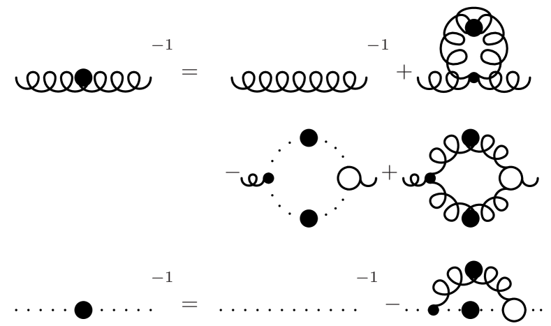
Figure 1: Graphical representation of the truncated system of vacuum DSEs. Wiggly lines represent gluons and dotted lines ghosts. Lines with a full dot are full propagators. Small dots denote bare vertices and open circles represent full vertices.

Finite temperature is introduced in the DSEs using the Matsubara formalism [19]. This entails two independent tensor structures for the gluon, one of them being three-dimensional (3d) transverse and the other one 3d longitudinal [20]

$$D_{\mu\nu}(q)=P_{T\mu\nu}(q)\frac{Z(q_{0}^{2},\vec{q}^{2})}{q^{2}}+P_{L\mu\nu}(q)\frac{H(q_{0}^{2},\vec{q}^{2})}{q^{2}}\;.$$ (5)

Therefore there are two independent dressing functions, $Z$ and $H$. The variable $q_{0}$ denotes the Matsubara frequency and $\vec{q}$ the spatial momentum. Note that Lorentz invariance, although not manifestly visible any more, is not lost in this formalism [21]. The ghost propagator, as a scalar, does not acquire a second independent dressing function. It depends nevertheless also on $q_{0}$ and $\vec{q}$ separately. Therefore three independent functions of two variables each have to be determined.

To obtain from the matrix equation for the gluon propagator two scalar equations for the dressing functions, it is contracted with two tensors [4]

$$P_{L\mu\nu}^{\xi} = \xi P_{L\mu\nu}+(1-\xi)(1+\frac{q_{0}^{2}}{\vec{q}^{2}})\delta_{\mu 0}\delta_{0\nu}$$

$$P_{T\mu\nu}^{\zeta} = \zeta P_{T\mu\nu}+(1-\zeta)(\delta_{\mu\nu}-(1+\frac{q_{0}^{2}}{\vec{q}^{2}})\delta_{\mu 0}\delta_{0\nu}).$$ (6)

where $\xi$ and $\zeta$ are two parameters. They are connected to the truncation scheme and will also be discussed in subsection 3.3. $P_{L}$ and $P_{T}$ are defined as [20]

$$P_{T\mu\nu} = \delta_{\mu\nu}-\frac{q_{\mu}q_{\nu}}{\vec{q}^{2}}+$$ (7)

$$+\delta_{\mu 0}\frac{q_{0}q_{\nu}}{\vec{q}^{2}}+\delta_{0\nu}\frac{q_{\mu}q_{0}}{\vec{q}^{2}}-\delta_{\mu 0}\delta_{0\nu}(1+\frac{q_{0}^{2}}{\vec{q}^{2}})$$

$$P_{L\mu\nu} = P_{\mu\nu}-P_{T\mu\nu}.$$ (8)

Graphically these equations are represented in Fig. 2. The solutions for small temperatures below the phase transition are discussed in [5].

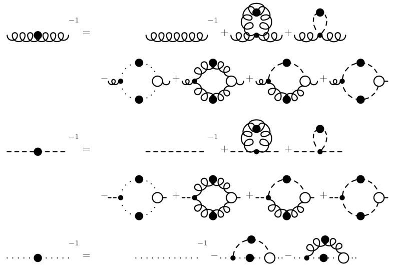
Figure 2: Graphical representation of the truncated system of DSEs at non-vanishing temperature. Wiggly lines represent 3d transverse gluons, dashed lines 3d longitudinal gluons and dotted lines ghosts. Lines with a full dot are full propagators. Small dots denote bare vertices and open circles represent the full vertices which have to be constructed in the truncation discussed in the text.

3.2 Dimensional Reduction

In the next step we take the infinite temperature limit of the truncated DSEs. To this end we note that, neglecting any contributions from Matsubara frequencies different from zero, this yields an effective three-dimensional Yang-Mills theory with an additional adjoint Higgs. This Higgs field is the remnant of the $A_{0}$ field in the four-dimensional theory. Thus the number of degrees of freedom is conserved.

The structure of the projectors (6) simplifies in the case of vanishing Matsubara frequency, i.e. $q_{0}=0$. $P_{L\mu\nu}^{\xi}$ becomes $\delta_{\mu 0}\delta_{0\nu}$ independent of $\xi$. It thus projects onto the time-time component of the propagator. Therefore, the 3d longitudinal part relates to the Higgs and this sector corresponds to the chromoelectric sector of the original theory. The non-vanishing elements of $P_{T\mu\nu}^{\zeta}$ become

$$P_{ij}^{\zeta}=\delta_{ij}-\zeta\frac{p_{i}p_{j}}{p^{2}}\;.$$ (9)

It projects onto the three-dimensional subspace. Therefore the gluons in the 3d reduced theory correspond to the chromomagnetic sector of the four-dimensional theory.

This dimensionally reduction amounts to integrating out the hard modes in tree-level approximation. Contributions from higher Matsubara frequencies can potentially generate additional terms in the Lagrangian of the dimensionally reduced theory [22]. Lattice calculations and matching in the perturbative regime show that this is indeed the case [22, 23]. Especially, a tree-level mass for the Higgs is generated. This also modifies the DSEs: the additional terms occurring stem from the neglected Matsubara frequencies and once included they can be derived from first principles as follows. The Lagrangian which governs the 3d reduced theory is [17, 22]

$${\cal L} = \frac{1}{4}F_{\mu\nu}^{a}F_{\mu\nu}^{a}+\bar{c}^{a}\partial_{\mu}D_{\mu}^{ab}c^{b}$$ (10)

$$+ \frac{1}{2}(D_{\mu}^{ab}\phi^{b}D_{\mu}^{ac}\phi^{c}+m_{h}^{2}\phi^{a}\phi^{a})+\frac{h}{4}\phi^{a}\phi^{a}\phi^{b}\phi^{b}$$

with the field strength tensor $F_{\mu\nu}^{a}$ and the covariant derivative $D_{\mu}^{ab}$ defined as

$$F^{a}_{\mu\nu} =\partial_{\mu}A_{\nu}^{a}-\partial_{\nu}A_{\mu}^{a}-g_{3}f^{abc}A_{\mu}^{b}A_{\nu}^{c}$$ (11)

$$D_{\mu}^{ab} =\delta^{ab}\partial_{\mu}+g_{3}f^{abc}A_{\mu}^{c}\;.$$ (12)

$A_{\mu}^{a}$ is the gauge field, $c^{a}$ the ghost, $\bar{c}^{a}$ the anti-ghost, $\phi^{a}$ the Higgs field, $g_{3}$ the dimensionful gauge coupling, $m_{h}$ is the Higgs mass, $h$ is the Higgs self-coupling and $f^{abc}$ the structure constants of the gauge group. A three-Higgs coupling is not present due to the antisymmetry of the structure constants and the remaining global color symmetry at tree-level.

If appropriate, multiples of $g_{3}^{2}$ are chosen as the fundamental scale and all results in the employed truncation scheme will be independent of $N_{c}$ for gauge groups SU($N_{c}$) in the following sense: In the chosen truncation scheme only the combination $C_{A}g_{3}^{2}$ appears as reference to the gauge group, $C_{A}=N_{c}$ being the second Casimir invariant of the adjoint representation of the group. Hence a change in $N_{c}$ can always be absorbed by a change in $g_{3}^{2}$ as long as the ratio $g_{3}^{2}/m_{h}$ is kept fixed.

The Higgs self-coupling $h$ can be uniquely determined in the 3d reduced theory. Since the Higgs field is a component of the four-dimensional gluon field, no linear divergence of the Higgs self-energy can occur due to the Slavnov-Taylor identities of the four-dimensional theory. Introducing temperature, no novel divergencies arise [19]. Implementation of this requirement fixes the Higgs self-coupling $h$ in leading-order perturbation theory (see appendix C).

All other constants occurring in the Lagrangian (10) are effective constants which arise by integrating out the heavy modes. For any large, although finite, temperature $T$ all remaining dimensionful quantities will scale as the temperature $T$. After rescaling, the precise dependence of $g_{3}$ on $T$ is irrelevant for the solution of the DSEs and the issue will be postponed to subsection 6.1.

The 3d reduced theory is not only superrenormalizable but finite, and all renormalization constants will be set to one in the following.

The DSEs for the Yang-Mills sector are already known, see e.g. [17]. They are rederived in appendix A for completeness. Since no tree level coupling between the Higgs and the ghost is present, the ghost equation will not be modified as compared to pure Yang-Mills theory. The ghost and the gluon DSEs are given by

$$(D_{G}^{-1})^{ab}(p) = -\delta^{ab}p^{2}$$ (13)

$$+ \int\frac{d^{d}q}{(2\pi)^{d}}\Gamma_{\mu}^{tl;c\bar{c}A;dae}(-q,p,q-p)D^{ef}_{\mu\nu}(p-q)$$

$$\qquad\times D^{dg}_{G}(q)\Gamma^{c\bar{c}A;bgf}_{\nu}(-p,q,p-q)\;,$$

$$(D_{H}^{-1})^{ab}(p) = \delta^{ab}(p^{2}+m_{h}^{2})+T^{HG;ab}+T^{HH;ab}$$ (14)

$$+ \int\frac{d^{d}q}{(2\pi)^{d}}\Gamma^{tl;A\phi^{2};eac}_{\nu}(-p-q,p,q)D_{\nu\mu}^{cg}(p+q)$$

$$\qquad\times D^{fc}(q)\Gamma_{\mu}^{gbf}(p+q,-p,-q)\;,$$

$$(D^{-1})^{ab}_{\mu\nu}(p) = \delta^{ab}(\delta_{\mu\nu}p^{2}-p_{\mu}p_{\nu})+T_{\mu\nu}^{GG;ab}+T^{GH;ab}_{\mu\nu}$$

$$- \int\frac{d^{d}q}{(2\pi)^{d}}\Gamma_{\mu}^{tl;c\bar{c}A;dca}(-p-q,q,p)D_{G}^{cf}(q)$$

$$\qquad\times D_{G}^{de}(p+q)\Gamma_{\nu}^{c\bar{c}A;feb}(-q,p+q,-p)$$

$$+ \frac{1}{2}\int\frac{d^{d}q}{(2\pi)^{d}}\Gamma^{tl;A^{3};acd}_{\mu\sigma\chi}(p,q-p,-q)D^{cf}_{\sigma\omega}(q)$$

$$\qquad\times D^{de}_{\chi\lambda}(p-q)\Gamma^{A^{3};bfe}_{\nu\omega\lambda}(-p,q,p-q)$$

$$+ \frac{1}{2}\int\frac{d^{d}q}{(2\pi)^{d}}\Gamma_{\mu}^{tl;A\phi^{2};acd}(p,q-p,-q)D^{de}(q)$$

$$\qquad\times D^{cf}(p-q)\Gamma^{A\phi^{2};bef}_{\nu}(-p,q,p-q)\;,$$

where $T^{i}$ are the tadpole contributions. The first label gives the equation where the tadpole contributes ($G$ for gluon and $H$ for Higgs) and the second the type of tadpole appearing. The index $tl$ denotes the tree-level quantities which are explicitely given in eqs.  (67) - (72) in appendix A. This set of 3d truncated equations is diagrammatically displayed in Fig. 3. Note that all momenta in these equations are three-momenta.

It is important to note that the ghost-gluon vertex function $\Gamma^{c\bar{c}A;abc}_{\nu}(p,q,-p-q)$ becomes bare for vanishing ghost momentum $p$ [2],

$$\lim_{p\to 0}\Gamma^{c\bar{c}A;abc}_{\nu}(p,q,-p-q)=ig_{3}f^{abc}q_{\nu}.$$ (16)

This identity especially ensures that we can choose a bare ghost-gluon vertex without altering qualitative results for the infrared behavior of the propagators. Indeed, at least in four dimensions, the qualitative nature of the infrared solution is independent of the detailed structure of the ghost-gluon vertex to a large extent [24]. Numerical consistency checks also find that the ghost-gluon-vertex does not depart significantly from its tree-level form [25]. Thus we will use a bare ghost-gluon vertex in the following. To complete the description of our truncation we still have to choose the 3-gluon vertex and the Higgs-gluon vertex. As these choices are motivated by more technical considerations we will defer all details concerning these vertex functions to the appropriate sections describing the numerical solutions.

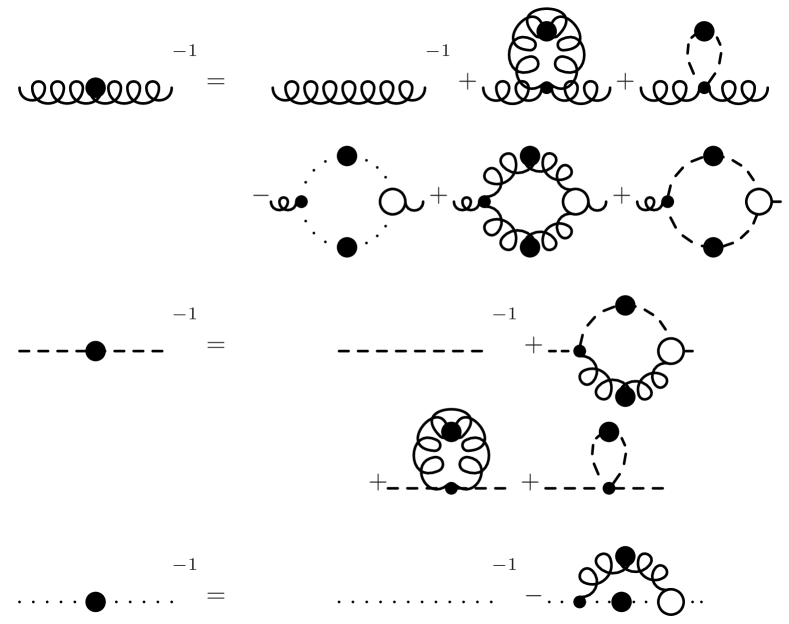
Figure 3: Graphical representation of the truncated system of DSEs in the infinite temperature limit. Wiggly lines represent gluons, dashed lines Higgs and dotted lines ghosts. Lines with a full dot are full propagators. Small dots denote bare vertices and open circles represent full vertices.

To obtain equations for the dressing functions, the color indices are contracted assuming the tree-level color structure for the vertex functions. This assumption is supported by lattice calculations [9]. The gluon DSE is transformed to a scalar equation by contracting it with the tensor (9). Dividing the DSEs by all trivial factors appearing on the l.h.s. these equations read

$${G^{-1}(p^{2})} = 1$$

$$+ \frac{g_{3}^{2}C_{A}}{4\pi^{2}}\int dqd\theta A_{T}(p,q)G(q^{2})Z((p-q)^{2})\;,$$

(17)

$${H^{-1}(p^{2})} = 1+\frac{m_{h}^{2}}{p^{2}}+T^{HG}+T^{HH}$$ (18)

$$+ \frac{g_{3}^{2}C_{A}}{4\pi^{2}}\int dqd\theta\Big{(}N_{1}(p,q)H(q^{2})Z((p+q)^{2})$$

$$\qquad+N_{2}(p,q)H((p+q)^{2})Z(q^{2})\Big{)}\;,$$

$${Z^{-1}(p^{2})} = 1+T^{GH}+T^{GG}$$ (19)

$$+ \frac{g_{3}^{2}C_{A}}{4\pi^{2}}\int dqd\theta\Big{(}R(p,q)G(q^{2})G((p+q)^{2})$$

$$\qquad+M_{L}(p,q)H(q^{2})H((p+q)^{2})$$

$$\qquad+M_{T}(p,q)Z(q^{2})Z((p+q)^{2})\Big{)}\;,$$

where $\theta$ is the angle between $p$ and $q$. For the truncation used in the present investigation, the integral kernels $A_{T}$, $N_{1}$, $N_{2}$, $R$, $M_{L}$ and $M_{T}$ are given in appendix B.

3.3 Constraints on the solutions

Due to the truncation of the DSEs, the Slavnov-Taylor identities are not fulfilled. This violation manifests itself in the appearance of spurious divergences in the gluon self-energy. These can be removed by adjusting either the tadpole terms or by projecting the gluon equation with the tensor (9) and choosing $\zeta=d=3$ in the equation for the 3d transverse gluon propagator [26]. The violation of gauge invariance does not manifest itself in the Higgs equation (14) of the 3d reduced theory. Thus this equation is independent of $\xi$. Furthermore, the Higgs self-energy in 3d is finite since the gluon propagator has only a logarithmic divergence in four dimensions. Therefore the divergencies of the two tadpole terms in (14) have to cancel each other exactly. Nonetheless, as the Higgs has a finite mass, the tadpoles involving a Higgs propagator have a finite contribution which correspond to a finite mass renormalization. This has to be taken into account and will be discussed in detail in section 4.

Varying $\zeta$ while selecting the tadpoles to cancel any spurious divergencies in the Yang-Mills and the Higgs sector of the gluon equation (LABEL:gluon) allows to explore different degrees of gauge violations. Especially the physical case of a transverse projected equation is of interest. If the results do not depend qualitatively and only weakly quantitatively on the value of $\zeta$ it is justified to assume that the effect of the violation of gauge symmetry is small and under control, c.f. refs. [27].

There is another aspect of gauge invariance to be respected in non-perturbative calculations. As the Lorentz condition does not completely fix the gauge field, configurations are over-counted. This is known as the Gribov problem [28]. The region of gauge space which contains no copies and includes the origin is called the fundamental modular region, see e.g. [29]. There is, however, at present no local condition known which defines this region. It is contained in the first Gribov region including the origin and configurations for which the Faddeev-Popov determinant does not change sign. The restriction to the first Gribov region can be formulated at the level of dressing functions as boundary conditions to the solutions of the DSEs as

$$G(q^{2})\geq 0,\quad Z(q^{2})\geq 0,\quad H(q^{2})\geq 0.$$ (20)

The condition on $H$ does not follow from the Gribov condition in three dimensions but only due to the fact that it is a component of the gauge field in four dimensions. The condition (20) does not completely solve the problem since the first Gribov horizon encloses a larger part of gauge space than the fundamental modular region, and therefore contains gauge copies [30]. Nevertheless, for the purpose of calculating propagators it is likely that this condition is sufficient for eliminating Gribov copies [15]. Note that, in lattice calculations, the Gribov ambiguity poses a more severe problem and makes it especially hard to extract the ghost propagator [31].

4 Infrared and ultraviolet behavior of the propagators

4.1 Ultraviolet behavior

The 3d reduced theory is also asymptotically free [32]. Thus the propagators and vertex functions reduce to their tree-level values for sufficiently large momenta. As the 3d reduced theory is finite, corrections are power-like. (In the case of the Higgs this is only true for $k\gg m_{h}$.) Since $g_{3}^{2}$ has the dimension of a mass and does not enter in the loop integrals of eqs. (17), (18) and (19), already by dimensional analysis, one infers that the one-loop contributions are proportional to $g_{3}^{2}/q$. Thus all loop integrals are subleading in the ultraviolet compared to the tree-level contribution. An explicit verification of this behavior is given in appendix C. Leaving aside the possibility of a finite renormalization, one has

$$\lim_{q^{2}\to\infty}G(q^{2})=\lim_{q^{2}\to\infty}Z(q^{2})=\lim_{q^{2}\to\infty}H(q^{2})=1.$$ (21)

For large enough $q^{2}$ the dressing functions are thus approximately given by

$$1+\frac{c_{i}g_{3}^{2}}{\sqrt{q^{2}}}$$ (22)

where the constants $c_{i}$ turn out to be positive for all dressing functions. Hence all dressing functions approach the tree-level behavior from above.

4.2 Infrared behavior

In this subsection we will study the infrared behavior of the dressing functions employing the following general ansätze:

$$G(q) = A_{g}q^{-2g},$$ (23)

$$Z(q) = A_{z}q^{-2t},$$ (24)

$$H(q) = A_{h}q^{-2l}.$$ (25)

For a pure Yang-Mills theory (without a Higgs) and a transversal projected gluon DSE this analysis has already been performed for three space-time dimensions in ref. [33].

The assumption $g=t=0$ and $l=-1$, motivated by the naive idea of a free gas of quarks and gluons in the high-temperature limit, immediately leads to a contradiction due to divergencies in the ghost and the gluon DSEs. Thus no such ’Coulomb phase’ can be realized when taking into account condition (16) on the ghost-gluon vertex. Also $g=0$ and $t=l=-1$, corresponding to a purely perturbative quark-gluon plasma with screening masses in the magnetic and the electric sector, immediately leads to a contradiction. This is also understood from the fact that, in order to obtain such a behavior, the tadpoles would have to dominate. However, for $\zeta=3$, the tadpole in the gluon equation does not contribute. Besides, it is hard to see how the vacuum corresponding to such propagators avoids the violation of Elitzur’s theorem [34] (for further details see ref. [35]). Hence the tadpole cannot be the infrared leading term in the gluon equation and one must have $t\leq-1$. Convergence of the integrals in the DSEs even requires $t<-1$, see appendix E. This is in agreement with the reasoning [15] for infrared dominance of the gauge fixing part of the Lagrangian (10). The inequality

$$t<-1$$ (26)

implies condition (1) and thus gluon confinement. On the one hand, this is no surprise as one expects confinement also in the three-dimensional Yang-Mills theory. On the other hand, it means that real-world chromomagnetic gluons are confined even at infinitely high temperatures! Note that the solution found in ref. [33] also obeys the inequality (26).

In appendix E the infrared limit of the DSEs is derived:

$$\frac{y^{g}}{A_{g}} = y^{-(d-4)/2-g-t}I_{GT}(g,t)A_{g}A_{z}$$ (27)

$$\frac{y^{t}}{A_{z}} = 1+y^{-(d-4)/2-2g}I_{GG}(g,\zeta)A_{g}^{2}$$ (28)

$$\frac{y^{l}}{A_{h}} = 1+\frac{m_{h}^{2}+\delta m^{2}}{y}.$$ (29)

where $y=q^{2}$ and $d$ denote the dimension. A subtraction in (27) has been performed and only the finite part is retained. The expressions for $I_{GT}$ and $I_{GG}$, originating from the ghost-self energy and the ghost-loop, can be found in appendix E. In the Higgs equation, a finite renormalization of the mass has been allowed for. The mass renormalization is given in equation (89) and is discussed in [35]. Eq. (29) possesses only one solution, namely $l=-1$ and

$$A_{h}=\frac{1}{m_{h}^{2}+\delta m^{2}}.$$ (30)

This indicates firstly a qualitative change in the high-temperature limit (as in four dimensions at $T=0$ one has $t=l$) and secondly the decoupling of the Higgs in the infrared. These observations agree with corresponding findings on the lattice [23].

The infrared ghost equation (27) implies the relation (see also [33])

$$g=-\frac{1}{2}(t+\frac{4-d}{2})=_{d\to 3}\;\;-\frac{1}{2}(t+\frac{1}{2}).$$ (31)

The difference to the relation in four dimensions

$$g=_{d\to 4}\;\;-t/2$$ (32)

implies an additional power in momentum which exactly compensates the dimension of the effective coupling constant in three dimensions. A corresponding compensation is expected at high temperatures in four dimensions to cancel the straightforward temperature factor in front of the Matsubara sum.

Due to the inequality (26) $g$ is positive. Thus any solution automatically satisfies (2) and both, the Kugo-Ojima and the Zwanziger-Gribov conditions, are fulfilled.

Using (31) in Eq. (28) one obtains

$$-\Big{(}2^{2g-d}\sqrt{\pi}(\frac{d}{2}+g)(2+d(\zeta-2)-4g(\zeta-1)-\zeta)$$

$$\times\csc(\frac{\pi(d-4g)}{2})\sin(\pi g)\Gamma(\frac{d}{2}+g)\Big{)}\Big{/}$$

$$\Big{/}\Big{(}(d-1)^{2}g\Gamma(\frac{1+d-2g}{2})\Gamma(2g)\Big{)}$$

$$=1.$$ (33)

This equation has at least one solution for $d\geq 1$ and two solutions for $d\geq 2$, see Fig. 4. Eq. (33) simplifies for $d=3$ to

$$1=\frac{32g(1-g)(1-\cot^{2}(g\pi))}{(1+2g)(3+2g)(2+2g(\zeta-1)-\zeta)}.$$ (34)

One of the two solutions in $d=3$ is independent of the projection of the gluon DSE:

$$(g,t)=(\frac{1}{2},-\frac{3}{2})$$ (35)

while the other one depends on the parameter $\zeta$. In the special case of a transverse projection, $\zeta=1$, one has

$$(g,t)=(0.3976,-1.2952)$$ (36)

thus reproducing the results of ref. [33] where only the case $\zeta=1$ has been treated.

Figure 4: The upper panel shows the two solutions for the ghost exponent $g$ for values of $\zeta$ allowed by condition (20) and integral convergence, see Eq. (92) and ref. [33]. This excludes the second branch in $d=2$. The dashed line is for $d=2$, the solid line for $d=3$ and the dashed-dotted line for $d=4$. The lower panel displays the two solutions for the ghost exponent $g$ as a function of $d$ for $\zeta=1$.

Condition (20), the inequality (26) as well as convergence of the integrals in the infrared restrict $g$ in three dimensions to

$$\frac{1}{4}<g\leq\frac{3}{4}.$$ (37)

Requiring furthermore a well-defined Fourier transform of the ghost propagator (at least in the sense of a distribution) leads to the condition $g\leq 1/2$. This restricts the range of allowed $\zeta$-values for the varying branch to

$$1/4\leq\zeta<3.$$ (38)

At the lower boundary both solutions merge into one.

Since in Eqs. (27) and (28) the prefactors $A_{g}$ and $A_{z}$ only appear in the product $A_{g}^{2}A_{z}$ only this combination is determined by the infrared analysis:

$$\frac{1}{A_{z}A_{g}^{2}} = \frac{C_{A}g_{3}^{2}}{(4\pi)^{\frac{3}{2}}}$$

$$\times\frac{2^{4(g-1)}(2+2g(\zeta-1)-\zeta)\Gamma(2-2g)\sin^{2}(\pi g)}{\cos(2\pi g)(g-1)g^{2}\Gamma(\frac{3}{2}-2g)}.$$

Determining these pre-factors turns out to be an essential and unexpectedly complicated part of the numerical method. Thus Eq. (LABEL:ag) is used to check whether a correct numerical solution is found [36].

5 Numerical Results

The numerical solution of the DSEs (17), (18) and (19) will be achieved in three steps: First, we study the ghost-loop only truncation where only diagrams with at least one ghost propagator are kept. Second, we include the gluon loop in the gluon equation. This truncation scheme neglects all Higgs contributions and thus corresponds to a purely three-dimensional Yang-Mills theory. The last step is then to fully implement the complete system. A description of the numerical method is given in refs. [35, 36].

5.1 Ghost-loop-only truncation

Keeping only ghost loops and using a bare ghost-gluon vertex, the system of DSEs is completely specified. The results of the corresponding calculation with $\zeta=3$, for both the ghost and the gluon dressing functions, are shown in Fig. 5. In this case, only the $g=1/2$ infrared solution exists. The gluon propagator exhibits a maximum located at $k/g_{3}^{2}\approx 0.25$.

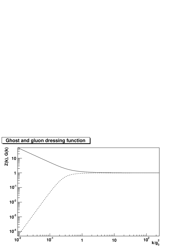
Figure 5: The solutions of the DSEs in the ghost-loop-only truncation scheme at $\zeta=3$. The dashed line refers to the dressing functions of the gluon $Z$ and the solid line to that of the ghost $G$. All quantities have been made dimensionless by dividing out appropriate powers of $g_{3}^{2}$.

The coupling constant is the only dimensionful quantity entering the DSEs. Thus all results can be represented through dimensionless variables when expressed in appropriate powers of $g_{3}^{2}$. Due to this fact, one can infer from Fig. 5 the results of the ghost-loop-only truncation for any positive value of the coupling constant. Even for a very small coupling constants strong non-perturbative effects for momenta smaller than $g_{3}^{2}$ are clearly visible. Therefore, the infrared behavior of the pertinent 2-point functions is never perturbative.

For $\zeta\neq 3$, a spurious divergence appears in the ghost loop of the gluon DSE. To cancel it, an appropriately adjusted tadpole term $T^{GG}$ is included. A subtlety required here comes from the fact that the subtraction due to the tadpole is only effective in the ultraviolet and not in the infrared. A detailed account of this subtraction is given in ref. [35] and the tadpole term $T^{GG}$ is given in appendix D. The solutions for the transverse projection ($\zeta=1$) are displayed in Fig. 6. In this case, solutions for both sets of infrared exponents exist. As in the case $\zeta=3$, the solutions show no special features.

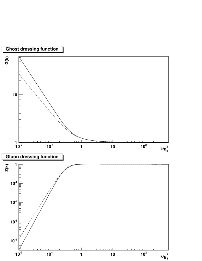
Figure 6: The ghost and gluon dressing function at $\zeta=1$. The upper panel shows the ghost dressing function, the lower panel shows the gluon dressing function. The solid line denotes the solution for $g=1/2$ and the dashed line gives the other solution branch with $g\approx 0.4$.

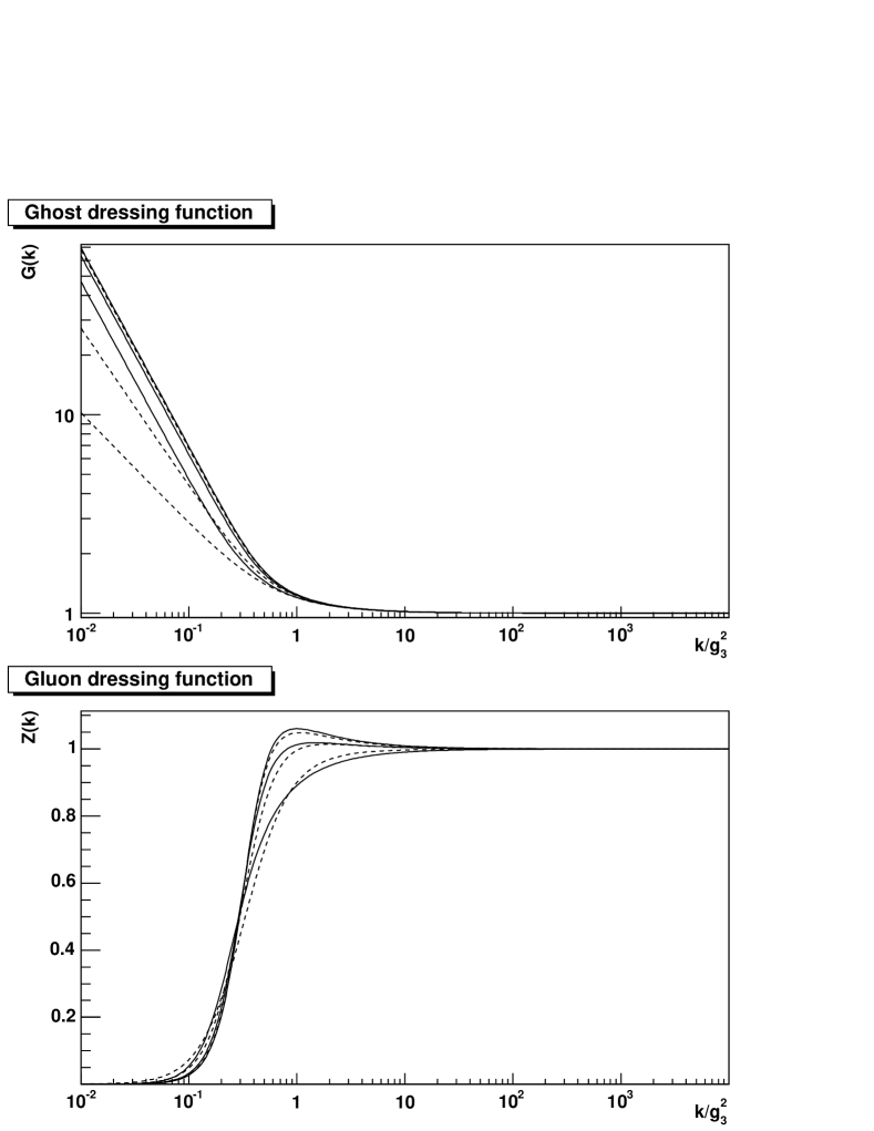
Figure 7: The ghost and gluon dressing function in ghost-loop-only approximation for different values of $\zeta$. The upper panel shows the ghost dressing function, the lower panel the gluon dressing function. The solid lines represent the solutions with a ghost infrared exponent, $g=1/2$, and the dashed lines the ones for the other set of infrared exponents. At the peak in the gluon, the middle lines correspond to solutions at $\zeta=1$. The upper and lower line at mid-momenta give the solutions at $\zeta=0$ and $4$ for the $g=1/2$-branch and at $\zeta=0.25$ and $2.55$ for the other branch.

To estimate the amount of gauge symmetry violation, the DSEs have been solved for different values of $\zeta$, see Fig. 7. To this end we have varied $\zeta$ between 0 and 4 for the set of half-integer infrared exponents. For the other branch, due to numerical uncertainties, $\zeta$ has only been varied from 0.25 to 2.55, the later corresponding to $g=0.2708$ and $t=-1.042$. Within the explored ranges the dependence of the solutions on $\zeta$, i.e. on the projection of the gluon DSE, is reasonably weak.

5.2 Yang-Mills theory

Figure 8: Solution of the Yang-Mills sector at $\zeta=3$. The dashed curve gives the ghost-loop-only solution for comparison. The solid curve gives the full Yang-Mills solution at $\delta=1/4$. Note the linear scale for $Z$ in the lower panel.

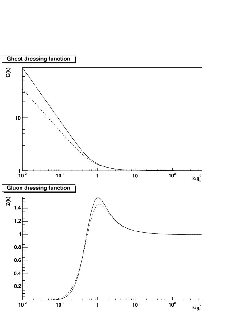
Figure 9: Solution of the Yang-Mills sector at $\zeta=1$. The upper panel shows the ghost dressing function and the lower panel the gluon dressing function. The solid curve denotes the $g=1/2$ solution while the dashed curve displays the $g\approx 0.4$ solution. Both are at $\delta=1/4$.

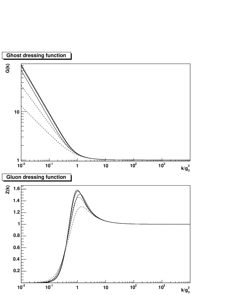
Figure 10: The ghost and gluon dressing of the pure Yang-Mills theory for different values of $\zeta$. The upper panel shows the ghost dressing function, and the lower panel the gluon dressing function. The solid line gives the solution for $g=1/2$ and the dashed line is for the other solution branch. At the peak in the gluon dressing function, the middle lines represent the solution at $\zeta=1$. The upper and lower lines at mid-momenta give the solutions at $\zeta=0$ and $\zeta=4$ for the $g=1/2$-branch and at $\zeta=1/4$ and $\zeta=2.45$ for the other solution branch.

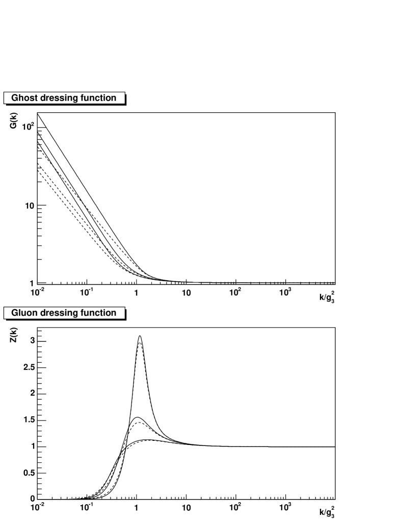
Figure 11: The ghost and gluon dressing functions of the pure Yang-Mills theory for different values of $\delta$. The upper panel shows the ghost dressing function, and the lower panel the gluon dressing function. The solid line gives the solution for $g=1/2$ and the dashed line is the other solution branch. At the peak in the gluon dressing function, the middle lines represent the solution at $\delta=1/4$. The upper and lower lines at mid-momenta give the solutions at $\delta=0.131$ and $\delta=1$ for the $g=1/2$-branch and at $\delta=0.114$ and $\delta=1$ for the other solution branch.

The gluon loop with a bare 3-gluon vertex in the gluon DSE contributes with opposite sign as the ghost-loop. This is correct in the ultraviolet and irrelevant in the infrared where it is subleading. At momenta of the order of $g_{3}^{2}$ the gluon loop calculated with a bare 3-gluon vertex becomes dominant. This leads to zeros on the r.h.s. of the gluon DSE and thus to a violation of the Gribov condition (20). Therefore, within this truncation scheme, the tree-level 3-gluon-vertex is not acceptable. Reasons might be that at momenta around $g_{3}^{2}$ (i) the bare 3-gluon-vertex overestimates the true vertex, (ii) the bare ghost-gluon vertex underestimates the true one and/or (iii) the two-loop graphs are important. These possibilities will be explored in more detail in future work [25]. However, as for the present study the specific reason for this shortcoming is of minor importance, we proceed by constructing an improved 3-gluon vertex. In this we are guided by earlier studies in four dimensions [7, 8] where minimal modifications have been introduced to obtain the correct ultraviolet behavior. To respect the Bose symmetry of the 3-gluon vertex we model it by multiplying the bare 3-gluon vertex with an appropriate product of functions. This leads to the ansatz

$$\Gamma^{A^{3}}_{\beta\sigma\mu}(-q,q+k,-k)\to$$

$$\Gamma_{\beta\sigma\mu}^{tl;A^{3}}(-q,q+k,-k)\;\left(A(q^{2})A((q+k)^{2})A(k^{2})\right)^{-\delta}\;,$$

$$A(q^{2})=Z(q^{2})(G(q^{2}))^{2+1/2g}.$$ (40)

The function $A$ is chosen to be a constant in the infrared. The additional parameter $\delta$ does not change this behavior. On the other hand, it allows to smoothly interpolate between a large suppression and the tree-level value by tuning it from large positive values to zero. Stable solutions have been found for $\delta\geq 0.114$. In the following, we employ mostly $\delta=1/4$ which yields a mild suppression of the 3-gluon vertex without effecting the stability of the numerical calculation.

The resulting dressing functions, using $\zeta=3$, are shown in comparison to the ghost-loop-only result in Fig. 8. For $\zeta\not=3$ tadpole terms have again to be subtracted. Their construction is detailed in ref. [35] and the corresponding expressions are given in appendix D. The results for $\zeta=1$ and $\delta=1/4$ are shown in Fig. 9. The dependence on $\zeta$ which provides a measure of gauge invariance violation, can be inferred from Fig. 10 and the one on $\delta$ from Fig. 11. The only qualitative difference in these functions, when compared to the ones of the ghost-loop-only truncation, is a maximum in the gluon dressing function which is now present for all employed values of $\zeta$. The location and height of this maximum depends on the vertex construction. For most values of $\delta$ this dependence is weak, however. Nevertheless, we have to conclude that the behavior of the dressing functions is sensitive to the structure of the 3-gluon vertex and additional information about this vertex function is highly desirable and will be studied in the future. In the context of this paper we will rely on the comparison to lattice data (see subsection 5.4) to justify our ansatz.

Being confident that these technical issues do not invalidate our results we note that the infrared behavior of the gluon and ghost propagators in three-dimensional Yang-Mills theory is very similar to the ones within four-dimensional Yang-Mills theory. Differences are of minor, quantitative nature. This is not surprising since the three-dimensional Yang-Mills theory is expected to be also a strongly interacting, confining theory [32].

5.3 Including the Higgs

Finally, we add the Higgs, i.e. we implement the full system of equations (17), (18) and (19). Although the Higgs loop in the gluon DSE provides a positive contribution it is not sufficient to allow for solutions with a bare 3-gluon vertex. Thus, the ansatz (40) will also be used for the full system. On the other hand, the tree-level gluon-Higgs vertex will be employed in this section. (In subsection 6.2 also a modified gluon-Higgs vertex will be studied.)

As stated already, a tree level Higgs mass is induced when integrating out the higher Matsubara modes in the process of dimensional reduction [22]. For the current analysis, the origin and the exact value of the Higgs mass are not of direct importance. Hence this mass will be fixed to a value extracted from lattice calculations and we use $m_{h}/g_{3}^{2}=0.8808$ [23] in the following.

As can be inferred from Fig. 2 three additional tadpole contributions arise when the Higgs is included, see also appendix A. Since the Higgs has a tree-level mass, two of the tadpoles can already have a non-vanishing finite part in leading-order perturbation theory, see appendix C. The self-energy of a Higgs field in a three-dimensional theory would be in general linearly divergent. This is not the case here. The Higgs, being a component of the gluon field in the four-dimensional theory, protects its self-energy from being divergent at the expense of fixing at leading-order perturbation theory the tree-level coupling $h$ to be

$$h=-2g_{3}^{2}\frac{C_{A}}{C_{A}+2},$$ (41)

see appendix C.

As can be seen from Fig. 12, the influence of the Higgs on the Yang-Mills sector is small. This is in agreement with results from lattice calculations [23]. The resulting Higgs propagator, see Fig. 13, behaves similar to a massive tree-level propagator.

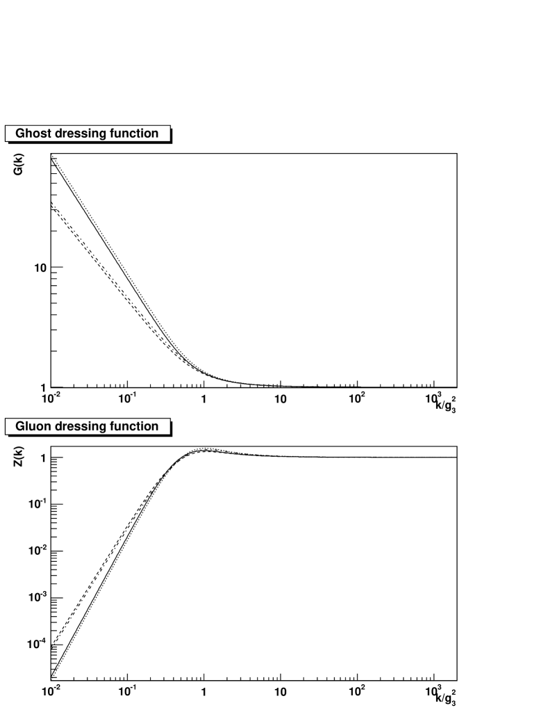
Figure 12: The solution of the Yang-Mills system compared to the full system at $\zeta=1$. The solid line denotes the full solution at $g=1/2$ while the dotted line is the corresponding Yang-Mills solution. The dashed line gives the full solution for the $g\approx 0.4$ solution while the dashed-dotted line is the corresponding Yang-Mills solution.

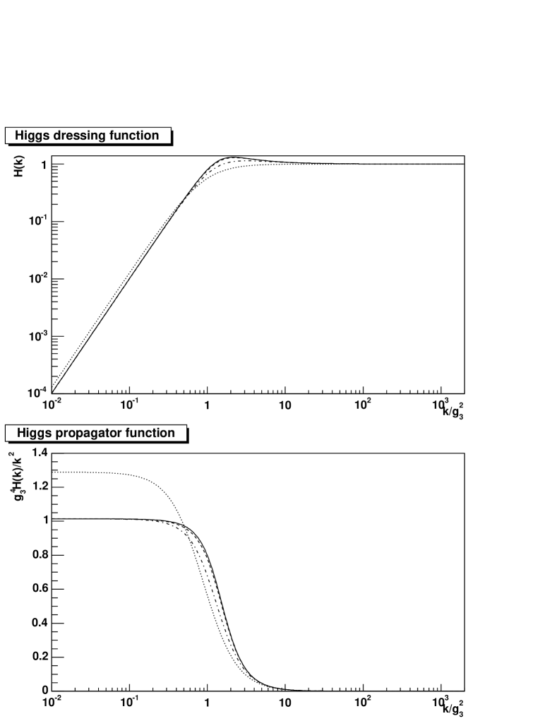
Figure 13: The Higgs dressing function and propagator at $\zeta=1$. The solid line gives the solution for $g=1/2$, the dashed line for $g\approx 0.4$, the dashed-dotted line denotes the leading-order perturbative result and the dotted line the tree-level behavior.

Although the Higgs mass is fixed in the current setting to be $m_{h}=0.8808g_{3}^{2}$, the Higgs mass dependence of the gluon and ghost propagators, especially for decreasing values of the Higgs mass, would be of interest. However, already after a slight decrease in the Higgs mass, the solution ceases to exist. For masses below $m_{h}\approx 0.6g_{3}^{2}$ no solution is found (at least, for $\delta\leq 1$).

The dependence of the Higgs on $\zeta$ is very small, deviations between solutions for different values of $\zeta$ not exceeding more than a few percent. However, the Higgs dressing function, at momenta $k\approx g_{3}^{2}$, is sensitive to the parameter $\delta$, see Fig. 14. Similar to what happens in the gluon dressing function, also the maximum of the Higgs dressing function increases with decreasing $\delta$. This is understandable from the fact that the Higgs self-energy depends on the strength of the gluon propagator.

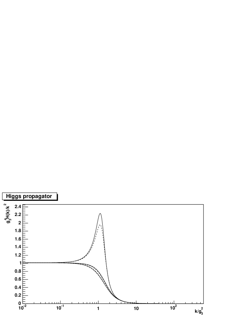
Figure 14: The Higgs propagator as a function of $\delta$ at $\zeta=1$. The solid line denotes the solution for $g=1/2$ and the dashed line for $g\approx 0.4$. The higher the peak the smaller $\delta$. The lowest peak corresponds to $\delta=1$, the middle one to $\delta=1/4$ and the largest one to $\delta=0.0862$ and $\delta=0.061$, respectively.

Although the analysis reveals some dependence on the parameters $\zeta$ and $\delta$ at intermediate momenta, it is important to note that infrared properties are only weakly dependent on these superficial quantities. Only one of the two exponents depends mildly on $\zeta$ as already discussed. In Fig. 15 we display the infrared coefficient $A_{g}$ as function of $\zeta$ or $\delta$. (Note that $A_{h}$ is fixed by the renormalized mass and $A_{z}$ depends uniquely on $A_{g}$.) Besides some dependence on $\delta$ for small values of this parameter (where the solutions cease to exist, as well) the infrared coefficients are rather robust up to the edges of numerical stability.

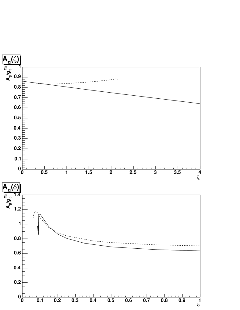
Figure 15: The dependence of the infrared coefficient $A_{g}$ on $\zeta$ in the upper panel and on $\delta$ in the lower panel. Solid lines represent the $g=1/2$ solution and dashed lines the other solution branch.

5.4 Comparison to lattice results

Recently lattice results for the gluon and the Higgs propagator [23] have become available. As the gluon propagator shows almost no sensitivity to the Higgs, not only in our but also in these lattice calculations, we additionally compare to the gluon propagator computed within three-dimensional lattice Yang-Mills theory [37].

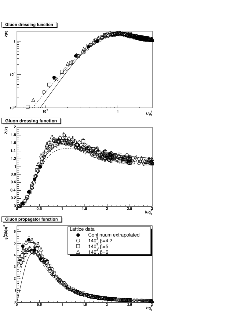
Figure 16: The gluon propagator and dressing function in pure Yang-Mills theory from the lattice and from subsection 5.2. The continuum-extrapolated values are from [23], the others from [37]. The errors indicated are statistical. The solid line denotes the $g=1/2$ solution and the dashed line the $g\approx 0.4$ solution. Both are at $\zeta=1$ and $\delta=1/4$.

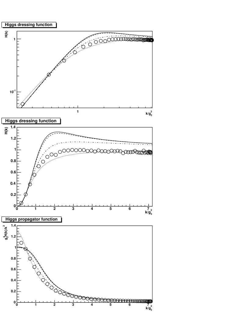
Figure 17: The Higgs propagator and dressing function in the full theory from the lattice and from subsection 5.3. The lattice data are from [23]. The errors indicated are statistical. The solid lines give the $g=1/2$ solution and the dashed lines the $g\approx 0.4$ solution, both at $\zeta=1$ and $\delta=1/4$. The dotted lines represent the tree-level result while the dashed-dotted lines give the leading-order perturbative results.

As can be inferred from Fig. 16, our results for the gluon propagator agree astonishingly well with the corresponding lattice results. As for the infrared behavior, the lattice results are in favor of the $g\approx 0.4$ solution. Note that, at momenta $k\approx g_{3}^{2}$, our truncation scheme is not trustworthy and the better agreement of the $g=1/2$ solution with the lattice gluon dressing function is not conclusive. As displayed in Fig. 17 the DSE results for the Higgs propagator show clear deviations from the corresponding lattice results, the latter being closer to the leading-order perturbative results than to the DSE results. We will return to a discussion of this point in subsection 6.3.

6 Towards observables

In a first step towards a calculation of observables from the propagators we determine an approximative form of the thermodynamic potential. Furthermore, we investigate screening masses via the calculation of the Schwinger functions from the propagators. In the following, the results for $\zeta=1$, $\delta=1/4$ and $C_{A}=N_{c}=3$ will always be used.

6.1 Thermodynamic potential

Knowledge of all Green’s functions as functions of the temperature would allow to calculate the thermodynamic potential and therefore all thermodynamic quantities. Since not all of these are known, it is not possible to calculate an exact thermodynamic potential. Knowledge of the propagators is however sufficient to compute an approximation to the thermodynamic potential, the Luttinger-Ward or Cornwall-Jackiw-Tomboulis (LW/CJT) effective action [38].

This effective action can be extended to abelian and non-abelian gauge theories, see e.g. [39, 40]. Its calculation is, however, prohibitively complicated when using constructed instead of bare or exact vertices. Therefore we will only extract here some qualitative features using the simplest approximation to the thermodynamic potential. It only depends on the propagators, and one has

$$\Omega= \frac{1}{2}d(G)T\sum\int\frac{d^{3}p}{(2\pi)^{3}}\Big{(}-\ln(Z(q))+(Z(q)-1)$$ (42)

$$+\ln(G(q))-(G(q)-1)$$

$$-\frac{1}{2}\ln(\frac{H(q)}{H_{0}(q)})+\frac{1}{2}(\frac{H(q)}{H_{0}(q)}-1)\Big{)}.$$

where $d(G)=\delta^{aa}$ is the dimension of the gauge group. $H_{0}$ is the tree-level Higgs dressing function

$$H_{0}(q)=\frac{q^{2}}{q^{2}+m_{h}^{2}}\;.$$ (43)

Working in the infinite-temperature limit we are eventually interested in the energy density divided by $T^{4}$. This motivates a rescaling of the integration momenta and one obtains

$$\frac{\Omega}{T^{4}}=\frac{g_{3}^{6}}{T^{3}}a$$ (44)

where the dimensionless constant $a$ depends only on the dimensionless ratio $m_{h}/g_{3}^{2}$ and thus becomes independent of temperature in the limit $T\to\infty$. In the simplest case, $g_{3}^{2}\sim g_{4}^{2}(\mu)T$ with the four dimensional coupling constant $g_{4}$ depending on the renormalization scale $\mu$. Herein enters the way in which the limit $T\to\infty$ is performed. When keeping $g_{3}(\mu)$ fixed by appropriately choosing $\mu(T)$, one has $g_{3}^{2}\sim\Lambda_{QCD}$. Hence (44) scales as $1/T^{3}$ and does not contribute to the thermodynamic pressure significantly compared to the hard modes. The Stefan-Boltzman behavior must then be obtained from the hard modes alone, requiring

$$\frac{\Omega}{T^{4}}=g^{6}_{4}(\mu)\bigl{(}a+\frac{b}{g_{4}^{6}(\mu)}\bigr{)}=\frac{g_{3}^{6}}{T^{3}}a+b$$ (45)

where $b$ stems from the hard modes [35]. However, the soft modes may still contribute significantly to thermodynamic properties, especially the trace anomaly, near the phase transition [41].

The calculation of (42) turns out to be plagued by spurious divergences, since the DSEs with the modified 3-gluon-vertex are no longer exact stationary solutions of (42). After carefully subtracting these [35], $a$ turns out to be within errors of ${\cal O}(1)$, but significantly depending on the truncation and large numerical uncertainties. The best value for the full solution is 3.6 for the $g=1/2$ solution and 3.5 for the $g\approx 0.4$ solution, contributed mostly from the Higgs-sector. The difference of two phases can be extracted with better accuracy, as the leading spurious divergence cancels. The result is

$$a_{g=1/2}-a_{g\approx 0.4}=0.053~{}.$$ (46)

Thus the $g\approx 0.4$ solution is thermodynamically preferred, in agreement with the lattice results in subsection 5.4.

6.2 Schwinger functions

Screening masses are most directly extracted from the analytic structure of the propagators. To obtain access to these analytic properties we calculate the Schwinger function related to the propagator $D$, defined as [10]

$$\Delta(t)=\frac{1}{\pi}\int_{0}^{\infty}dp_{0}\cos(tp_{0})D(p_{0}),$$ (47)

i.e. the Fourier transform of the propagator with respect to (Euclidean) time. Note that this definition is independent of the dimensionality of the underlying theory. Negative values for the Schwinger function can be traced to violations of positivity and therefore to absence of the particle, represented by $D$, from the physical spectrum [10].

Using a sufficiently sophisticated FFT-algorithm together with at least 512 or more frequencies, it is possible to calculate the Schwinger functions. The result for the gluon, presented in Fig. 18, clearly exhibits positivity violations. This is in accordance with the Oehme-Zimmermann super-convergence relation (1) and thus has been expected. Furthermore, the position of the zeros can be interpreted as the confinement scale. For the $g=1/2$ solution, the zero occurs at $g_{3}^{2}t\approx 3.29$ and at $g_{3}^{2}t\approx 3.98$ for the other branch. This result is in agreement with recent lattice results [42].

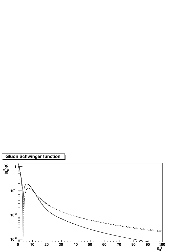
Figure 18: The Schwinger function of the gluon. The solid line gives the numerical result for $g=1/2$ while the dashed line is for $g\approx 0.4$. The dotted and dash-dotted line denote their respective fits using the ansatz (6.2).

To be able to perform an analytic continuation of the gluon propagator into the complex $q^{2}$-plane we first fit the Schwinger function. This is performed by using the ansatz

$$Z_{f}(q) =\frac{A_{z}q^{4g+1}}{1+f+A_{z}q^{4g+1}}(1+\frac{f}{1+fa_{u}q})$$

$$=\frac{A_{z}q^{4g+1}(1+f+a_{u}fq)}{(1+a_{u}fq)(1+f+A_{z}q^{4g+1})}$$

for the dressing function. $A_{z}$ is the infrared coefficient determined previously, and $a_{u}$ is the ultraviolet coefficient of leading-order resummed perturbation theory, as calculated in appendix C. The fit parameters for both solutions are given in table 1. As demonstrated in Fig. 18 the Schwinger function is fitted very well. The gluon propagator and dressing function are also reasonably well described by the fit, see Fig. 19.

Solution	$A_{z}g_{3}^{-2t}$	$a_{u}g_{3}^{2}$	$f$
$g=1/2$	20.3	$64/27$	1.32511
$g\approx 0.4$	13.4	$64/27$	1.03148

Table 1: The coefficients for the gluon fit (6.2).

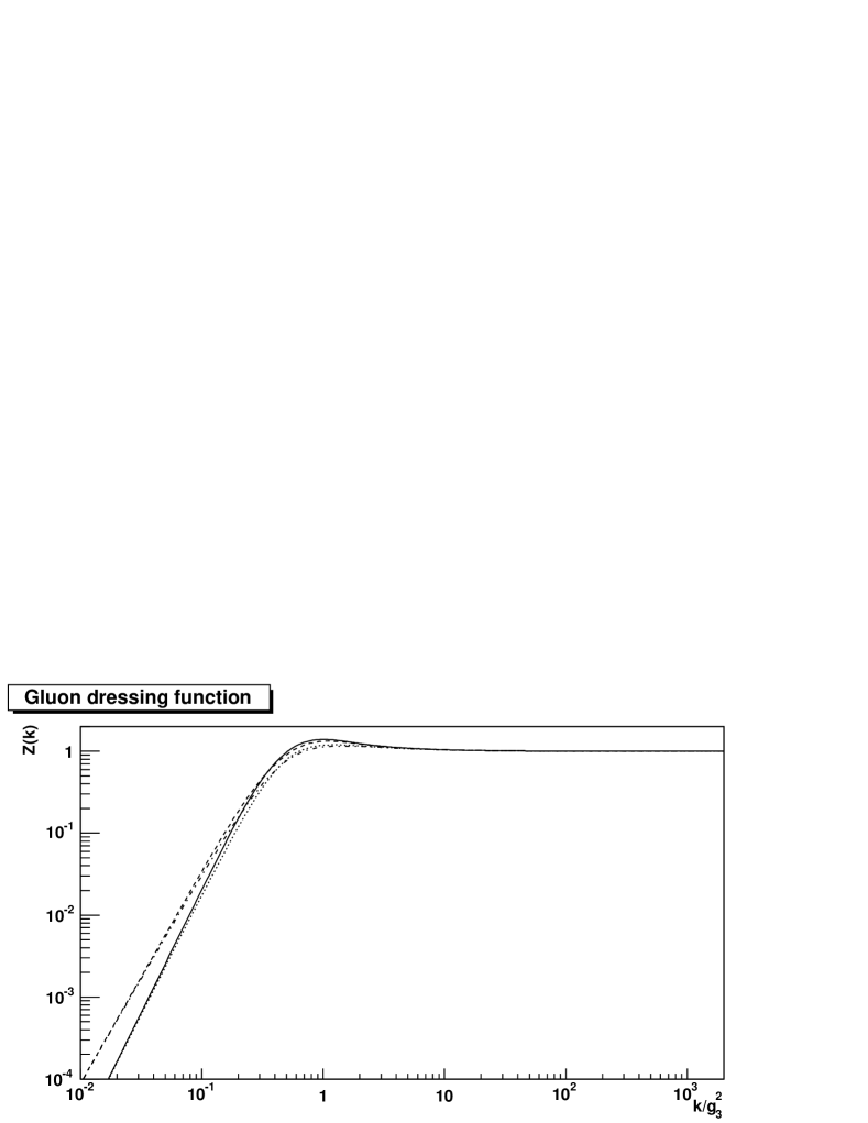
Figure 19: Comparison of the fit-function (6.2) to the full solutions of the dressing function. The solid line indicates the $g=1/2$ solution and dotted line its fit. The dashed line represents the $g\approx 0.4$ solution and the dashed-dotted line its fit.

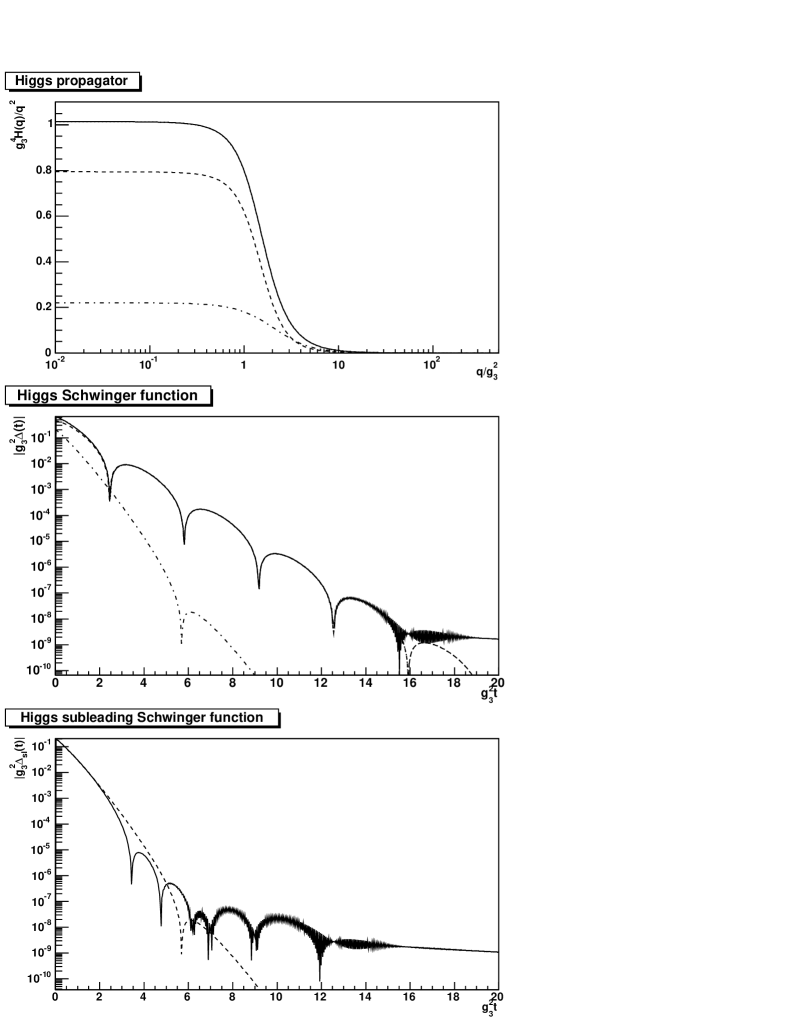
Figure 20: The Higgs propagator in the top panel and its Schwinger function in the middle panel compared to their fits for $g=1/2$. The solid lines represent the numerical solution, the dashed lines give the leading contribution and the dashed-dotted lines the first subleading contribution. The dotted lines underneath the solid lines give the sum of the leading and subleading contribution. The bottom panel shows the comparison of the numerical (solid) and the fitted (dashed) subleading Higgs contribution, see text.

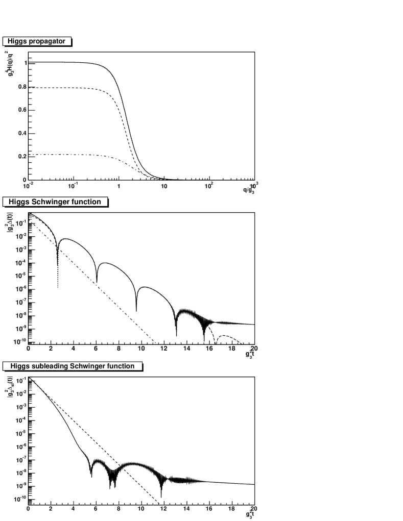
Figure 21: The Higgs propagator in the top panel and its Schwinger function in the middle panel compared to their fits for $g\approx 0.4$. The solid lines represent the numerical solution, the dashed lines give the leading contribution and the dashed-dotted lines the first subleading contribution. The dotted lines underneath the solid lines give the sum of the leading and subleading contribution. The bottom panel shows the comparison of the numerical (solid) and the fitted (dashed) subleading Higgs contribution, see text.

Similar to a meromorphic fit ansatz used in ref. [10] we will describe the Higgs propagator and its Schwinger function, the latter being analytically calculated from the former, as follows

$$H_{f}(q)=\frac{e+fq^{2}}{q^{4}+2m^{2}\cos(2\phi)q^{2}+m^{4}}\;,$$ (49)

$$\Delta_{f}(t)=\frac{e}{2m^{3}\sin(2\phi)}e^{-tm\cos(\phi)}$$

$$\times(\sin(\phi+tm\sin(\phi))+\frac{fm^{2}}{e}\sin(\phi-tm\sin(\phi)))\;.$$

As demonstrated in Figs. 20 and 21 these fits already describe the Schwinger function quite well, but miss around 20% of the propagator at zero momentum. This indicates that further massive modes are present. Indeed, for the $g=1/2$ solution, a further term of the form (49) has to be added. For the $g\approx 0.4$ solution, adding a term with one pole,

$$H_{f}(q)=\frac{e}{q^{2}+m^{2}}\;,$$ (50)

$$\Delta_{f}(t)=\frac{e}{2m}e^{-mt}\;,$$

allows to improve the fit in this case, as well. Both subleading fits are not very accurate for large $t$, and the results have to be taken with care. They indicate, nevertheless, the existence of subleading contributions due to the presence of further massive-particle-like contributions. The fit parameters of both solutions can be found in table 2.

Solution	$e$	$fg_{3}^{4}$	$\phi$	$m/g_{3}^{2}$
$g=1/2$	4.0199	0.3545	-0.67078	1.4998
subleading	9.4493	0.6736	-0.18387	2.561
$g\approx 0.4$	4.0697	0.37793	-0.63975	1.5045
subleading	0.81188			1.9223

Table 2: The coefficients for the Higgs fit (49) and the subleading one (49) and (50), respectively.

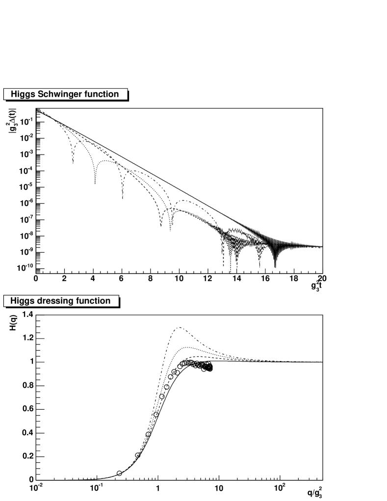
Figure 22: The top panel shows the Higgs propagator of the $g\approx 0.4$ solution for various suppression factors $\omega$ of the Higgs-gluon vertex. The bottom panel shows the corresponding Schwinger functions. The lattice data are the same as in fig. 17. The solid line is for $\omega=1/4$, the dashed line for $\omega=1/2$, the dotted line is for $\omega=3/4$ and the dashed-dotted line for $\omega=1$.

As can be seen from fig. 17 the result for the Higgs propagator deviates significantly from the lattice results, the self-energy being significantly overestimated. While the gluon Schwinger function is reasonably independent of the truncation, this turns out not to be the case for the Higgs Schwinger function. In order to show this we study the solution for a bare Higgs-gluon vertex suppressed via a scaling factor $\omega$. First, we note that the gluon Schwinger function, in contrast to the Higgs one, is not susceptible to such a change.

Fig. 22 displays corresponding results for different values of $\omega$. The position of the first zero tends to increase for decreasing $\omega$. At $\omega\approx 1/4$ any oscillation, at least within the available numerical precision, seems to be gone altogether. A fit to the Schwinger function using (50) reveals again additional structure at very small $t$ which cannot be captured by such a simple fit. As the fit also does miss some strength at zero momentum for the propagator this again indicates the presence of further massive contributions in the propagator.

6.3 Analytic properties

Although the high-temperature limit of the four-dimensional Minkowski theory is a genuinely Euclidian theory, it will be of interest for other applications to extract the analytic structure of the propagators investigated.

The gluon propagator exhibits similar behavior for both solutions but there are also some significant differences. The denominator of the ansatz (6.2) contains two factors, both of which could possibly give rise to a non-trivial analytic structure. The first part stems from the fit of the perturbative tail necessary to generate the maximum in the gluon dressing function. Since all fit parameters are positive, this factor does not give rise to a pole on the first Riemann sheet. However, it generates a pole on the second Riemann sheet, which will occur at $1/a_{u}f$, that is, at Euclidian momenta. This pole does not have a physical interpretation, and may well be an artifact of the fit, since (6.2) is tailored to generate the correct leading-order perturbative behavior. Thus it generates most likely a structure which has the Landau pole of perturbation theory on the second Riemann sheet. We expect that this pole vanishes when using a more sophisticated fit.

The second factor generates a genuine isolated pole at $(-(1+f)/A_{z})^{-1/t}$. This expression has only one value on the first Riemann sheet given by $(-0.0933+0.1615i)g_{3}^{4}$ for the $g=1/2$ and $(-0.1462+0.1248i)g_{3}^{4}$ for the other solution. In both cases a pole close to the origin is generated with an imaginary part larger than the real part in one case. For the first solution, the pole is found for an angle significantly above $\pi/4$ while in the second case somewhat below. In addition, the first solution generates two more poles on two more Riemann sheets, while the second solution, with a (most likely) irrational exponent, generates an infinite number of further poles on an infinite number of Riemann sheets. In both cases, the residue is complex. In addition, there is a cut along the complete negative real axis starting at zero. In this way it is similar to the results in four dimensions [10].

From this analysis we infer that the gluon propagator is positivity violating, and thus satisfies the requirements of the Kugo-Ojima and Zwanziger-Gribov confinement scenario.

Solution	Order	Pole$/g_{3}^{4}$
$g=1/2$	Leading	$-0.5112\pm 2.191i$
$g=1/2$	Subleading	$-6.11972\pm 2.35777i$
$g\approx 0.4$	Leading	$-0.650078\pm 2.16822i$
$g\approx 0.4$	Subleading	$-3.69539$

Table 3: Location of the poles of the Higgs propagator for $\omega=1$.

On the other hand, the Higgs propagator very likely does not have a branch cut but a number of simple poles whose locations are given in table 3. The sensitivity to the Higgs-gluon vertex, however, necessitates further investigations before a firmer conclusion can be drawn. We only note here that for smaller values of the suppression factor $\omega$ the Higgs propagator agrees better with lattice results, and its poles are then close to or on the real axis.

7 Discussion

Eqs. (17), (18) and (19) describe the infinite-temperature limit of Landau-gauge Yang-Mills theory. The resulting gluon propagator exhibits the characteristic behavior of a confined particle. The Yang-Mills subsector is satisfying both, the Kugo-Ojima scenario (1) and the Zwanziger-Gribov scenario (2), thus describing a confined theory. These properties are very stable against the assumptions made: the result of confined gluons is nearly independent of the truncation and of the properties of the Higgs. Hence, in accordance with corresponding lattice results, the presence of long-range chromomagnetic forces is found.

The chromoelectric sector is simpler in that it is close to a perturbative behavior. However, as the comparison to lattice calculations shows, at least next-to-leading-order perturbative effects or even genuinely non-perturbative effects play a role.

Combing these findings with the results from the vacuum [7] and from the low-temperature calculations [5] has impact on the understanding of the phase transition. The main difference between the low and the high-temperature phase is not primarily one between a strongly interacting and confining system and one with only quasi-free particles. The chromoelectric gluons, whose infrared behavior change from over-screening to screening, comes somewhat close to such a picture. The chromomagnetic gluons stay over-screened in the infrared and thus confined. The order parameter for the phase transition is then necessarily only a chromoelectric one. From the studies of Wilson loops it is known that only the temporal (electric) Wilson lines show a behavior typical of deconfinement while the spatial (magnetic) ones do not [43]. Note that the order parameters used to study the deconfinement transition on the lattice are typically chromoelectric ones like the Polyakov lines [3]. Using the corresponding magnetic Polyakov lines we conjecture that almost no change will be found. This point of view is also supported by recent lattice calculations [44] which observe even at $6T_{c}$ an over-screened magnetic and a screened electric propagator, albeit on rather small lattices.

The results presented here may have also consequences for the thermodynamic potential. In the analysis of the Higgs propagator indications for further particle-like poles have been found. These could contribute to the pressure. The way in which over-screened gluons contribute to the energy density but not to the pressure has been very recently discussed in ref. [41].

Another topic related to the investigations presented here is the recently established connection between four-dimensional Yang-Mills theory in Coulomb gauge and three-dimensional Yang-Mills theory in Landau gauge [46]. The time-time component of the Coulomb-gauge gluon propagator is on the one hand directly linked to the static quark-quark potential and on the other hand to the connected parts of expectation values of the Faddeev-Popov operator. From this one concludes that the potential is approximatively given by the ghost dressing function. The infrared behavior of the Coulomb-gauge ghost propagator in four dimensions and the Landau-gauge ghost propagator in three dimensions are determined from identical equations and one obtains identical infrared exponents. While the solution $g\approx 0.4$ generates a potential which behaves as $\sim 1/k^{3.6}$ and is thus a little less than linear with distance, the second branch generates a solution proportional to $1/k^{4}$ for small momenta, thus generating the behavior expected for a linear confining potential.

8 Conclusions and Outlook

We have analyzed the DSEs of three-dimensional Yang-Mills theory with and without an additional massive adjoint Higgs field and solved them in a given truncation scheme. The investigated theory can be regarded as the high-temperature limit of a four-dimensional Yang-Mills theory. Besides the propagators we considered the corresponding Schwinger functions. Although the resulting Higgs function behaves nearly perturbative it does not have a simple structure and experiences higher-order or even non-perturbative effects. The chromomagnetic gluons are over-screened. The Faddeev-Popov ghost propagator is infrared enhanced similar to the four-dimensional one. The corresponding long-range correlations thus imply confinement of chromomagnetic modes as they imply confinement of transverse gluons in four dimensions.

We have given an approximate expression for the thermodynamic potential. At the current stage it allows to discriminate which of the two sets of solutions is the preferred one. Of course, it is our goal to extend our formalism such that physical observables such as the energy density, pressure and entropy can be calculated reliably.

The next steps, however, also in connection with the results found in [5], will be to include the higher Matsubara frequencies to introduce the effects of a finite temperature into the system. This will hopefully allow us to determine the critical temperature and other aspects of the phase transition. Including quarks will allow to address the chiral phase transition. An extension to finite quark chemical potential is feasible  [18, 47], and thus investigations of the QCD phase diagram based on a calculation of the infrared behavior of QCD Green’s functions will become possible as well.

The authors are grateful to Christian S. Fischer for his help in the early stages of this work. They thank Michael Buballa, Peter Petreczky, Craig D. Roberts, and Daniel Zwanziger for valuable discussions and Attilio Cucchieri for a critical reading of the manuscript and helpful remarks. This work is supported by the BMBF under grant number 06DA917, by the European Graduate School Basel-Tübingen (DFG contract GRK683) and by the Helmholtz association (Virtual Theory Institute VH-VI-041).

Appendix A Derivation of the Dyson-Schwinger equations

The Dyson-Schwinger equations are the equations of motions for a quantum field theory. They can be derived [16, 17, 18] for the Euclidian version from

$$\left(\left(-\frac{\delta S}{\delta\phi^{a}(x)}|_{\phi=\frac{\delta}{\delta j^{a}(x)}}+j^{a}(x)\right)Z[j^{a}(x)]\right)_{j=0}=0$$ (51)

where $\phi$ is the field variable, $j$ the corresponding source term and $a$ a generic multi-index. $S$ is the Euclidian action and $Z$ is the generating functional,

$$Z=\int{\cal D}\phi^{a}e^{-S[\phi^{a}]+\int dx\phi^{a}(x)j^{a}(x)}$$ (52)

that can be written as $Z=\exp(W)$, $W$ being a function of the external sources. The effective action, i.e. the Legendre transform of $W$, is defined by

$$W(j^{a})=-\Gamma(\phi^{a})+\int d^{d}xj^{a}(x)\phi^{a}(x)$$ (53)

which implies

$$\phi^{a}=\frac{\delta W}{\delta j^{a}}\;,$$ (54)

$$j^{a}=\frac{\delta\Gamma}{\delta\phi^{a}}\;.$$ (55)

In the case of Grassmann fields, $c$, such as ghosts and fermions, two independent sources are necessary. This modifies the above to

$$Z=\int{\cal D}c^{a}{\cal D}\bar{c}^{a}e^{-S[c^{a},\bar{c}^{a}]+\int d^{d}x(\bar{\eta}^{a}(x)c^{a}(x)+\bar{c}^{a}(x)\eta^{a}(x))}$$ (56)

$$c^{a}(x)=\frac{\delta W}{\delta\bar{\eta}^{a}(x)}\quad\quad\quad\quad\bar{c}^{a}(x)=-\frac{\delta W}{\delta\eta^{a}(x)}$$

$$W(\eta^{a},\bar{\eta}^{a})$$

$$=-\Gamma(u^{a},\bar{u}^{a})+\int d^{d}x(\bar{\eta}^{a}(x)c^{a}(x)+\bar{c}^{a}(x)\eta^{a}(x))$$ (57)

$$\eta^{a}(x)=\frac{\delta\Gamma}{\delta\bar{c}^{a}(x)}\quad\quad\quad\quad\bar{\eta}^{a}(x)=-\frac{\delta\Gamma}{\delta c^{a}(x)}$$

where all derivatives with respect to Grassmann variables act in the direction of ordinary derivatives.

The general procedure to obtain the corresponding Dyson-Schwinger equations is to calculate the expression (51) for a given action and then perform once more a functional derivative with respect to the field or with respect to the conjugate field in case of anti-commuting fields. The additional source term then yields the propagator while the right-hand-side of the equations are found by the derivative of the action.

In general, propagators and their inverse are defined as

$$\frac{\delta^{2}\Gamma}{\delta\phi^{b}(y)\delta\phi^{a}(x)} =D^{ab}(x-y)^{-1}$$ (58)

$$\frac{\delta^{2}W}{\delta\phi^{b}(y)\delta\phi^{a}(x)} =D^{ab}(x-y)$$ (59)

while full $n$-point vertices are defined by a $n$-fold derivative of $\Gamma$. For the ghost-gluon vertex which is defined as

$$\frac{\delta^{3}\Gamma}{\delta c^{a}(x)\delta\bar{c}^{b}(y)\delta A^{c}_{\mu}(z)}=\Gamma_{\mu}^{c\bar{c}A;abc}(x,y,z)\;,$$ (60)

the sequence of derivatives is relevant (in contrast to the gluon vertex functions).

Using the identities

$$\frac{\delta^{2}W}{\delta j^{e}_{\mu}(x)\delta\bar{\eta}^{d}(x)}$$

$$=-\int d^{d}zd^{d}w\frac{\delta^{2}W}{\delta j_{\nu}^{f}(z)\delta j^{e}_{\mu}(x)}\frac{\delta^{2}\Gamma}{\delta\bar{c}^{g}(w)\delta A_{\nu}^{f}(z)}\frac{\delta^{2}W}{\delta\eta^{g}(w)\delta\bar{\eta}^{d}(x)}$$ (61)

$$\partial_{\mu}^{x}\frac{\delta}{\delta\eta^{c}(x)}=\int d^{d}z\Big{(}\partial_{\mu}^{x}\frac{\delta\Gamma}{\delta\eta^{c}(x)\delta\bar{c}^{e}(z)}\Big{)}\frac{\delta}{\delta\eta^{e}(z)}$$ (62)

$$\frac{\delta^{3}W}{\delta A_{\nu}^{b}(y)\delta j^{c}_{\sigma}(x)\delta^{e}_{\sigma}(x)}=$$

$$-\int dzdw\frac{\delta^{2}W}{\delta j_{\sigma}^{c}(x)\delta j_{\rho}^{f}(z)}\frac{\delta^{3}\Gamma}{\delta A_{\nu}^{b}(y)\delta A_{\rho}^{f}(z)\delta A_{\omega}^{g}(w)}\frac{\delta^{2}W}{\delta j_{\omega}^{g}(w)\delta j_{\sigma}^{e}(x)},$$ (63)

it is straightforward (although tedious) to derive the DSEs in position space. Performing a Fourier transformation to momentum space, where all momenta are defined as incoming and momentum conservation at the vertices is taken into account, the DSEs in momentum space are derived. To make the appearance of the tree-level vertices explicit, it is necessary to add in general permuted versions of each diagram and using the (anti-)symmetry of the vertices in their respective fields. The ghost propagator equation reads

$$D^{ab-1}_{G}(p)=-\delta^{ab}p^{2}$$

$$+\int\frac{d^{d}q}{(2\pi)^{d}}\Gamma_{\mu}^{tl;c\bar{c}A;dae}(-q,p,q-p)D^{ef}_{\mu\nu}(p-q)D^{dg}_{G}(q)\cdot$$

$$\cdot\Gamma^{c\bar{c}A;bgf}_{\nu}(-p,q,p-q)\;,$$ (64)

the gluon one is given by

$$D^{ab-1}_{\mu\nu}(p)=\delta^{ab}(\delta_{\mu\nu}p^{2}-p_{\mu}p_{\nu})$$

$$-\int\frac{d^{d}q}{(2\pi)^{d}}\Gamma_{\mu}^{tl;c\bar{c}A;dca}(-p-q,q,p)D_{G}^{cf}(q)D_{G}^{de}(p+q)\cdot$$

$$\cdot\Gamma_{\nu}^{c\bar{c}A;feb}(-q,p+q,-p)$$

$$+\frac{1}{2}\int\frac{d^{d}q}{(2\pi)^{d}}\Gamma^{tl;A^{3};acd}_{\mu\sigma\chi}(p,q-p,-q)D^{cf}_{\sigma\omega}(q)D^{de}_{\chi\lambda}(p-q)\cdot$$

$$\cdot\Gamma^{A^{3};bfe}_{\nu\omega\lambda}(-p,q,p-q)$$

$$+\frac{1}{2}\int\frac{d^{d}q}{(2\pi)^{d}}\Gamma_{\mu}^{tl;A\phi^{2};acd}(p,q-p,-q)D^{de}(q)D^{cf}(p-q)\cdot$$

$$\cdot\Gamma^{A\phi^{2};bef}_{\nu}(-p,q,p-q)$$

$$+\frac{1}{2}\int\frac{d^{d}q}{(2\pi)^{d}}\Gamma_{\mu\nu\sigma\rho}^{tl;A^{4};abcd}(p,-p,q,-q)D^{cd}_{\sigma\rho}(q)$$

$$+\frac{1}{6}\int\frac{d^{d}qd^{d}k}{(2\pi)^{2d}}\Gamma_{\mu\sigma\xi\chi}^{tl;A^{4};acde}(p,-q,-p+q-k,k)\cdot$$

$$\cdot D_{\chi\lambda}^{dh}(p-q-k)D_{\xi\rho}^{cf}(q)D_{\sigma\omega}^{eg}(k)\Gamma^{A^{4};hbfg}_{\lambda\nu\rho\omega}(p-q-k,-p,q,k)$$

$$+\frac{1}{2}\int\frac{d^{d}qd^{d}k}{(2\pi)^{2d}}\Gamma^{tl;A^{4};acde}_{\mu\delta\gamma\sigma}(p,-q,q-k-p,k)D_{\gamma\lambda}^{dh}(k+p-q)\cdot$$

$$\cdot\Gamma_{A^{3};\nu\rho\omega}^{bfg}(-p,p+k,-k)\Gamma_{A^{3};\lambda\chi\xi}^{hij}(k+p-q,q,-k-p)\cdot$$

$$\cdot D_{\rho\xi}^{fj}(p+k)D_{\sigma\omega}^{eg}(k)D_{\delta\chi}^{ci}(q)$$

$$+\frac{1}{2}\int\frac{d^{d}q}{(2\pi)^{d}}\Gamma^{tl;A^{2}\phi^{2};abdf}_{\mu\nu}(p,-p,q,-q)D^{df}(q)$$

$$-\frac{1}{2}\int\frac{d^{d}qd^{d}k}{(2\pi)^{2d}}\Gamma_{\mu\sigma}^{tl;A^{2}\phi^{2};aedf}(p,q-p-k,-q,k)D^{fi}(k)$$

$$\cdot D_{\sigma\rho}^{eg}(p-q+k)D^{dh}(q)\Gamma_{\rho\nu}^{A^{2}\phi^{2};gbhi}(p-q+k,-p,q,-k)$$

$$+\int\frac{d^{d}qd^{d}k}{(2\pi)^{2d}}\Gamma_{\mu\sigma}^{tl;A^{2}\phi^{2};aedf}(p,q-p-k,-q,k)D_{\mu\rho}^{eg}(p+k-q)\cdot$$

$$\cdot D^{fi}(k)D^{hk}(k+p)D^{dj}(q)\Gamma^{A\phi^{2};gjk}_{\rho}(p+k-q,q,-k-p)\cdot$$

$$\cdot\Gamma^{A\phi^{2};bhi}_{\nu}(-p,k+p,-k)\;,$$ (65)

and finally the one for the Higgs is

$$D^{ab}(p)^{-1}=\delta^{ab}(p^{2}+m_{h}^{2})$$

$$+\int\frac{d^{d}q}{(2\pi)^{d}}\Gamma^{tl;A\phi^{2};eac}_{\nu}(-p-q,p,q)D_{\nu\mu}^{cg}(p+q)\cdot$$

$$\cdot D^{fc}(q)\Gamma_{\mu}^{gbf}(p+q,-p,-q)$$

$$+\frac{1}{2}\int\frac{d^{d}q}{(2\pi)^{d}}\Gamma_{\mu\nu}^{tl;A^{2}\phi^{2};cdab}(q,-q,p,-p)D_{\mu\nu}^{cd}(q)$$

$$-\frac{1}{2}\int\frac{d^{d}qd^{d}k}{(2\pi)^{d}}\Gamma_{\mu\sigma}^{tl;A^{2}\phi^{2};cdae}(-p-q+k,-k,p,q)\cdot$$

$$\cdot D_{\mu\nu}^{cg}(p+q-k)D_{\rho\sigma}^{id}(k)D^{eh}(q)\cdot$$

$$\cdot\Gamma_{\rho\nu}^{A^{2}\phi^{2};igbh}(-k,p+q-k,-p,q)$$

$$+\frac{1}{2}\int\frac{d^{d}qd^{d}k}{(2\pi)^{2d}}\Gamma_{\mu\sigma}^{tl;A^{2}\phi^{2};cdae}(-q,k,p,-p+q-k)D_{\mu\nu}^{cg}\cdot$$

$$\cdot D^{ej}(p-q+k)(q)D_{\rho\sigma}^{id}(k)\Gamma_{\nu}^{A\phi^{2};gjk}(q,p-q+k,-p-k)\cdot$$

$$\cdot D^{kh}(p+k)\Gamma_{\rho}^{A\phi^{2};ibh}(-k,-p,p+k)$$

$$+\frac{1}{2}\int\frac{d^{d}qd^{d}k}{(2\pi)^{2d}}\Gamma_{\mu\chi}^{tl;A^{2}\phi^{2};cdae}(-q,q+k,p,-p-k)D^{cg}_{\mu\nu}(q)\cdot$$

$$\cdot D^{eh}(p+k)D_{\lambda\chi}^{kd}(q+k)\Gamma_{\sigma\nu\lambda}^{A^{3};jgk}(k,q,-q-k)\cdot$$

$$\cdot D_{\rho\sigma}^{ij}(k)\Gamma_{\rho}^{A\phi^{2};ibh}(-k,-p,p+k)$$

$$+\frac{1}{2}\int\frac{d^{d}q}{(2\pi)^{d}}\Gamma^{tl;\phi^{4};abcd}(p,-p,q,-q)D^{cd}(q)$$

$$-\frac{1}{6}\int\frac{d^{d}qd^{d}k}{(2\pi)^{2d}}\Gamma^{tl;\phi^{4};agch}(p,-p+q-k;k;-q)D^{he}(q)\cdot$$

$$\cdot D^{gd}(p-q+k)D^{fc}(k)\Gamma^{\phi^{4};debf}(p-q+k,q,-p,-k)$$

$$+\frac{1}{3}\int\frac{d^{d}qd^{d}k}{(2\pi)^{2d}}\Gamma^{tl;\phi^{4};aicj}(p,-p-k+q,k,-q)D^{id}(p+k-q)\cdot$$

$$\cdot D^{jg}(q)D^{fc}(k)\Gamma^{\phi^{3};gdh}(q,p+k-q,-k-p)\cdot$$

$$\cdot D^{eh}(p+k)\Gamma^{\phi^{3};ebf}(p+k,-p,-k)\;.$$ (66)

The tree-level vertices for the ghost-gluon-, 3-gluon-, 4-gluon-, 2-gluon-Higgs-, 2-gluon-2-Higgs- and 4-Higgs- interactions have been used. They are given by

$$\Gamma_{\mu}^{tl;c\bar{c}A;abc}(p,q,k) = ig_{3}f^{abc}q_{\mu}$$ (67)

$$\Gamma_{\mu\nu\rho}^{tl;A^{3};abc}(p,q,k) = -ig_{3}f^{abc}((q-k)_{\mu}\delta_{\nu\rho}+(k-p)_{\nu}\delta_{\mu\rho}$$ (68)

$$+(p-q)_{\rho}\delta_{\mu\nu})$$

$$\Gamma_{\mu\nu\sigma\rho}^{tl;A^{4};abcd}(p,q,k,l) = g_{3}^{2}(f^{eab}f^{ecd}(\delta_{\mu\sigma}\delta_{\nu\rho}-\delta_{\mu\rho}\delta{\nu\sigma})$$ (69)

$$+f^{gac}f^{gbd}(\delta_{\mu\nu}\delta_{\sigma\rho}-\delta_{\mu\rho}\delta_{\nu\sigma})$$

$$+f^{gad}f^{gbc}(\delta_{\mu\nu}\delta_{\sigma\rho}-\delta_{\mu\sigma}\delta_{\nu\rho}))$$

$$\Gamma_{\mu}^{tl;A\phi^{2};abc}(p,q,k) = ig_{3}f^{abc}(q-k)_{\mu}$$ (70)

$$\Gamma_{\mu\nu}^{tl;A^{2}\phi^{2};abcd}(p,q,k,l) = g_{3}^{2}\delta_{\mu\nu}(f^{eac}f^{ebd}+f^{ead}f^{ebc})$$ (71)

$$\Gamma^{tl;\phi^{4};abcd}(p,q,k,l) = 2h(\delta_{ab}\delta_{cd}+\delta_{ac}\delta_{bd}+\delta_{ad}\delta_{bc}),$$ (72)

where the momentum conserving $\delta$-functions have been suppressed. The complete graphical representation of (64), (65), and (66) is shown in Fig. 23.

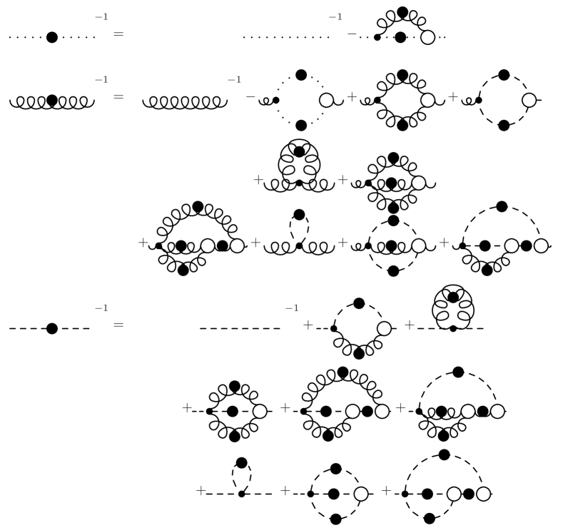
Figure 23: The DSEs of the propagators of the Yang-Mills theory with an adjoint Higgs given in (64), (65), and (66). The same conventions apply as in Fig. 3.

Appendix B Integral kernels

The integral kernels in eqs. (17), (18) and (19) are obtained by using tree-level vertices and performing the corresponding contractions. The ghost kernel is given by

$$A_{t}(k,q,\theta)=-\frac{q^{2}\sin^{3}(\theta)}{(k^{2}+q^{2}-2kq\cos\theta)^{2}}.$$ (73)

The contributions in the Higgs equation are

$$N_{1}(k,q,\theta)=-\frac{2q^{2}\sin^{3}(\theta)}{(k^{2}+q^{2}+2kq\cos\theta)^{2}}$$ (74)

$$N_{2}(k,q,\theta)=-\frac{2\sin^{3}(\theta)}{k^{2}+q^{2}+2kq\cos\theta}.$$ (75)

The kernels in the gluon equations are finally

$$R(k,q,\theta)=-\frac{((\zeta-1)kq\cos(\theta)-q^{2}+\zeta q^{2}\cos^{2}(\theta))\sin\theta}{2k^{2}(k^{2}+q^{2}+2kq\cos\theta)}$$ (76)

$$M_{L}(k,q,\theta)=$$

$$\frac{((\zeta-1)(k^{2}+4kq\cos\theta)-4q^{2}+4q^{2}\zeta\cos^{2}(\theta))\sin\theta}{4k^{2}(k^{2}+q^{2}+2kq\cos\theta)}$$ (77)

$$M_{T}(k,q,\theta)=\frac{\sin\theta}{4k^{2}(k^{2}+q^{2}+2kq\cos\theta)}\cdot$$

$$\cdot\Big{(}(k^{2}+2q^{2})((\zeta-9)k^{2}-4q^{2})+8(\zeta-3)(k^{2}+q^{2})kq\cos\theta$$

$$+(8\zeta q^{4}+(\zeta+7)k^{4}+4(5\zeta-1)k^{2}q^{2})\cos^{2}(\theta)$$

$$+4(4\zeta q^{2}+(\zeta+3)k^{2})\cos^{3}(\theta)+4\zeta k^{2}q^{2}\cos^{4}(\theta)\Big{)}$$ (78)

The modified gluon vertex is introduced by multiplying $M_{T}$ with (40).

Appendix C Perturbative expressions

Replacing all full quantities in the truncated DSEs (17), (18) and (19) by their tree-level values, i.e. one for all dressing functions and the tree-level vertices (67-72) instead of the full vertices, the standard perturbation theory to one-loop order is obtained. It is then possible to calculate the leading-order perturbative dressing functions. For the ghost this becomes

$$G(k)^{-1}=1-\frac{g_{3}^{2}C_{A}}{16k}$$ (79)

to leading order, independent on the presence of a Higgs. Note that a Landau pole at $k={\cal O}(g_{3}^{2})$ is present.

The calculation of the gluon self-energy is a little more tricky since, although finite in three dimensions due to a Slavnov-Taylor identity, each single contribution is linearly divergent. Corresponding problems are most easily circumvented when contracting the gluon equation with the Brown-Pennington projector. Performing the calculation in pure Yang-Mills theory yields

$$Z(k)^{-1}=1-\frac{11g_{3}^{2}C_{A}}{64k}.$$ (80)

Including the Higgs one obtains

$$Z(k)^{-1}=1-\frac{11g_{3}^{2}C_{A}}{64k}$$

$$+\frac{g_{3}^{2}C_{A}}{16\pi k}\Big{(}2\frac{m_{h}}{k}-\frac{k^{2}+4m_{h}^{2}}{k^{2}}\csc^{-1}\sqrt{1+\frac{4m_{h}^{2}}{k^{2}}}\Big{)}.$$ (81)

Since non-perturbative effects already arise at order $1/k^{2}$ in the present truncation scheme, the only interesting part is for $k\gg g_{3}^{2},m_{h}$ leading to

$$Z(k)^{-1}=1-\frac{9g_{3}^{2}C_{A}}{64k}.$$ (82)

Finally the Higgs self-energy is

$$H(k)^{-1}=1+\frac{m_{h}^{2}}{k^{2}}+\frac{g_{3}^{2}C_{A}}{k}\frac{m_{h}}{4\pi k}$$

$$+\frac{g_{3}^{2}C_{A}}{k}\frac{1}{2\pi k}\left(-m_{h}+\left(\frac{m_{h}^{2}+k^{2}}{k}-2k\right)\arcsin(\sqrt{\frac{k^{2}}{m_{h}^{2}+k^{2}}})\right)$$ (83)

where the third term is the tadpole contribution. The leading contribution is

$$H(k)^{-1}=1-\frac{g_{3}^{2}C_{A}}{4k}.$$ (84)

The coupling constant $h$ is determined by requiring that the sum of the tadpole kernels already generate a finite integral, i.e. independent of the regularization scheme. This is obtained by requiring (41).

Note that, in three dimensions, resummation has only effects from order $g_{3}^{4}$ on since, by dimensional arguments alone, only tree-level expressions in the loops can contribute at order $g_{3}^{2}$. Therefore (79), (82) and (84) already constitute the resummed solution. This is confirmed by the numerical calculations presented in section 5.

Note further that this also ensures that gauge symmetry is intact to one-loop order in the regime of applicability of leading-order resummed perturbation theory. The violation of gauge symmetry in this approach is, at least, not stronger than in ordinary leading-order perturbation theory.

Appendix D Tadpoles

The tadpoles used for the ghost-loop-only system read:

$$T^{GG}= -\frac{g_{3}^{2}C_{A}}{(2\pi)^{2}}\int dqd\theta\Big{(}R_{D}(k,q)(G(q)G(k+q)$$ (85)

$$-A_{g}^{2}q^{-2g}(k+q)^{-2g})+R_{3}(k,q)\big{(}G(q)G(k+q)$$

$$-A_{g}^{2}q^{-2g}(k+q)^{-2g}-1\big{)}\Big{)}.$$

Here the kernel $R$ has been split into its convergent, $\zeta$-independent part $R_{0}$, its finite $\zeta$-dependent part $R_{3}$ and its divergent part $R_{D}$ as

$$R=R_{0}+R_{3}+R_{D}.$$ (86)

For the pure Yang-Mills theory this is altered to

$$T^{GG}= -\frac{g_{3}^{2}C_{A}}{(2\pi)^{2}}\int dqd\theta\Big{(}R_{D}(k,q)(G(q)G(k+q)$$ (87)

$$-A_{g}^{2}q^{-2g}(k+q)^{-2g})$$

$$+R_{3}(k,q)\big{(}G(q)G(k+q)-A_{g}^{2}q^{-2g}(k+q)^{-2g}$$

$$-1\big{)}+M_{TD}(k,q)Z(q)Z(k+q)\Big{)},$$

where $M_{TD}$ contains the divergent part of $M_{T}$, including the alterations due to the dressed 3-gluon-vertex (40). For the full theory the additional tadpole in the gluon equation is given by

$$T^{GH}=-\frac{g^{2}C_{A}}{(2\pi)^{2}}\int dqd\theta\Big{(}M_{LD}(k,q)H(q)H(k+q)\Big{)}.$$ (88)

In the Higgs equation, the tadpoles are set to

$$T^{HG}+T^{HH}=\frac{g_{3}^{2}C_{A}}{k^{2}}\frac{m}{4\pi}=:\frac{\delta m^{2}}{k^{2}}.$$ (89)

A detailed account for the construction of the tadpoles is given in ref. [35].

Appendix E Infrared expressions

As already argued in section 4.2, the only solution without further assumption is that of ghost dominance. This then requires the calculation of $I_{GT}$ and $I_{GG}$ in (27) and (28) only. The latter can be obtained straightforwardly when using the ansatz (25) and the general formula

$$\int\frac{d^{d}q}{(2\pi)^{d}}x^{\alpha}z^{\beta}$$

$$=\frac{1}{(4\pi)^{\frac{d}{2}}}\frac{\Gamma(-\alpha-\beta-\frac{d}{2})\Gamma(\frac{d}{2}+\alpha)\Gamma(\frac{d}{2}+\beta)}{\Gamma(d+\alpha+\beta)\Gamma(-\alpha)\Gamma(-\beta)}y^{\frac{d}{2}+\alpha+\beta}$$ (90)

valid for finite integrals, where $x=q^{2}$, $z=(q-k)^{2}$ and $y=k^{2}$. It yields

$$I_{GG}=-\frac{g_{3}^{2}C_{A}\pi}{(4\pi)^{\frac{d}{2}}}\cdot$$

$$\cdot\frac{2^{4g-2d}(d-4g)(2+d(\zeta-2)-4g(\zeta-1)-\zeta)\Gamma(d-2g)\Gamma(2g-\frac{d}{2})}{(d-1)g^{2}\Gamma(\frac{1+d-2g}{2})^{2}\Gamma(g)^{2}}$$ (91)

Note that the integral is convergent iff

$$\frac{d-1}{2}\geq g>\frac{d-2}{4}$$ (92)

where the equality on the upper boundary requires the result to exist only in the sense of a distribution.

Performing the same calculation for the ghost self-energy is more complicated. Since it is, in general, a divergent quantity Eq. (90) cannot be applied directly. It is necessary to regularize and then renormalize the expression. This can be done in a momentum subtraction scheme [33] or via dimensional regularization. Here, the later has been performed by applying the standard rules of dimensional regularization [48]. This then immediately gives a finite result. However, by doing so a divergent quantity has been removed which is formally eliminated by setting $-\widetilde{Z}_{3}$ equal to this quantity. This procedure yields the same result as the momentum subtraction scheme. The range allowed for $g$ in (92) renders $I_{GT}$ not only to have a divergence of logarithmic or linear order in even or uneven dimensions, but also quadratic or cubic divergences. Using a subtraction scheme, it would be necessary to include the next term in the Taylor expansion. On the other hand, dimensional renormalization directly yields

$$I_{GT}=\frac{g_{3}^{2}C_{A}}{(4\pi)^{\frac{d}{2}}}\cdot$$

$$\cdot\frac{2^{1-2g}(4^{g}(d-3)d+2^{1+2g}(1+g-dg))\Gamma(\frac{d}{2}-g)\Gamma(-g)\Gamma(2g)}{(2-d+2g)(d+2g)\Gamma(\frac{d}{2}-2g)\Gamma(g)\Gamma(\frac{d}{2}+g)}$$ (93)

Note that this expression becomes negative already for values allowed by (92), e.g. for $g\geq 3/4$ in three dimensions, thus reducing the allowed range and leading to the plots in Fig. 4.

References

- [1] R. Alkofer, C. S. Fischer, H. Reinhardt and L. von Smekal, Phys. Rev. D 68 (2003) 045003 [arXiv:hep-th/0304134].
- [2] J. C. Taylor, Nucl. Phys. B 33 (1971) 436. W. J. Marciano and H. Pagels, Phys. Rept. 36 (1978) 137.
- [3] F. Karsch and E. Laermann, arXiv:hep-lat/0305025; and references therein.
- [4] A. Maas, B. Grüter, R. Alkofer and J. Wambach, Proceedings of the 40th International School of Subnuclear Physics, August 29th - September 7th, Erice, Italy, Ed.: A. Zichichi, World Scientific 2003; arXiv:hep-ph/0210178.
- [5] B. Grüter, R. Alkofer, A. Maas, J. Wambach, to be published; see also B. Grüter, R. Alkofer, A. Maas, J. Wambach, Proceedings of the Erice summer school on Nuclear Physics, Sept. 16 – 24, 2003, Erice, Italy; arXiv:hep-ph/0401164
- [6] F. J. Dyson, Phys. Rev. 75 (1949) 1736, J. S. Schwinger, Proc. Nat. Acad. Sci. 37 (1951) 452, Proc. Nat. Acad. Sci. 37 (1951) 455.
- [7] L. von Smekal, A. Hauck and R. Alkofer, Annals Phys. 267 (1998) 1 [arXiv:hep-ph/9707327]; L. von Smekal, R. Alkofer and A. Hauck, Phys. Rev. Lett. 79 (1997) 3591 [arXiv:hep-ph/9705242].
- [8] C. S. Fischer and R. Alkofer, Phys. Rev. D 67 (2003) 094020 [arXiv:hep-ph/0301094].
- [9] P. Boucaud, J. P. Leroy, J. Micheli, O. Pene and C. Roiesnel, JHEP 9812 (1998) 004 [arXiv:hep-ph/9810437]. P. Boucaud, J. P. Leroy, J. Micheli, O. Pene and C. Roiesnel, JHEP 9810 (1998) 017 [arXiv:hep-ph/9810322]. H. Nakajima and S. Furui, arXiv:hep-lat/0309165. S. Furui and H. Nakajima, arXiv:hep-lat/0309166.
- [10] R. Alkofer, W. Detmold, C. S. Fischer and P. Maris, Phys. Rev. D 70 (2004), 014014 [arXiv:hep-ph/0309077]; arXiv:hep-ph/0309078.
- [11] K. Osterwalder and R. Schrader, Commun. Math. Phys. 31 (1973) 83. K. Osterwalder and R. Schrader, Commun. Math. Phys. 42, 281 (1975).
- [12] R. Oehme and W. Zimmermann, Phys. Rev. D 21 (1980) 1661. R. Oehme and W. Zimmermann, Phys. Rev. D 21 (1980) 471.
- [13] T. Kugo and I. Ojima, Prog. Theor. Phys. Suppl. 66 (1979) 1.
- [14] T. Kugo, arXiv:hep-th/9511033.
- [15] D. Zwanziger, Phys. Rev. D 69 (2004) 016002 [arXiv:hep-ph/0303028].
- [16] R. J. Rivers, “Path Integral Methods In Quantum Field Theory” (Cambridge University Press, Cambridge, 1987).
- [17] R. Alkofer and L. von Smekal, Phys. Rept. 353 (2001) 281 [arXiv:hep-ph/0007355].
- [18] C. D. Roberts and S. M. Schmidt, Prog. Part. Nucl. Phys. 45 (2000) S1 [arXiv:nucl-th/0005064].
- [19] A. K. Das, “Finite Temperature Field Theory” (World Scientific, Singapore, 1997).
- [20] J. I. Kapusta, “Finite Temperature Field Theory” (Cambridge University Press, Cambridge, 1989).
- [21] H. A. Weldon, Phys. Rev. D 26 (1982) 1394.
- [22] K. Kajantie, M. Laine, K. Rummukainen and M. E. Shaposhnikov, Nucl. Phys. B 458 (1996) 90.
- [23] A. Cucchieri, F. Karsch and P. Petreczky, Phys. Rev. D 64 (2001) 036001 [arXiv:hep-lat/0103009].
- [24] C. Lerche and L. von Smekal, Phys. Rev. D 65 (2002) 125006 [arXiv:hep-ph/0202194].
- [25] W. Schleifenbaum, A. Maas, J. Wambach, R. Alkofer (in preparation)
- [26] N. Brown and M. R. Pennington, Phys. Rev. D 38 (1988) 2266.
- [27] C. S. Fischer and R. Alkofer, Phys. Lett. B536, 177 (2002) [arXiv:hep-ph/0202202]; C. S. Fischer, R. Alkofer and H. Reinhardt, Phys. Rev. D65, 094008 2002 [arXiv:hep-ph/0202195]; R. Alkofer, C. S. Fischer and L. von Smekal, Acta Phys. Slov. 52, 191 (2002) [arXiv:hep-ph/0205125]; C. S. Fischer, PhD thesis, U. of Tuebingen, arXiv:hep-ph/0304233.
- [28] V. N. Gribov, Nucl. Phys. B 139 (1978) 1.
- [29] D. Zwanziger, Nucl. Phys. B 412 (1994) 657.
- [30] P. van Baal, arXiv:hep-th/9711070.
- [31] A. Cucchieri, Nucl. Phys. B 521 (1998) 365. T. D. Bakeev, E. M. Ilgenfritz, V. K. Mitrjushkin and M. Mueller-Preussker, arXiv:hep-lat/0311041.
- [32] R. P. Feynman, Nucl. Phys. B 188 (1981) 479.
- [33] D. Zwanziger, Phys. Rev. D 65 (2002) 094039 [arXiv:hep-th/0109224].
- [34] S. Elitzur, Phys. Rev. D 12 (1975) 3978.
- [35] A. Maas, PhD thesis, Darmstadt University of Technology end of 2004, to be published
- [36] A. Maas (in preparation)
- [37] A. Cucchieri, T. Mendes and A. R. Taurines, Phys. Rev. D 67 (2003) 091502 [arXiv:hep-lat/0302022].
- [38] J. M. Luttinger and J. C. Ward, Phys. Rev. 118 (1960) 1417; J. M. Cornwall, R. Jackiw and E. Tomboulis, Phys. Rev. D 10 (1974) 2428.
- [39] B. J. Haeri, Phys. Rev. D 48 (1993) 5930 [arXiv:hep-ph/9309224].
- [40] M. E. Carrington, G. Kunstatter and H. Zaraket, arXiv: hep-ph/0309084. M. E. Carrington, arXiv:hep-ph/0401123.
- [41] D. Zwanziger, arXiv:hep-ph/0407103.
- [42] A. Cucchieri, T. Mendes and A. R. Taurines, arXiv:hep-lat/0406020.
- [43] G. S. Bali, J. Fingberg, U. M. Heller, F. Karsch and K. Schilling, Phys. Rev. Lett. 71 (1993) 3059 [arXiv:hep-lat/9306024].
- [44] A. Nakamura, T. Saito and S. Sakai, Phys. Rev. D 69 (2004) 014506 [arXiv:hep-lat/0311024].
- [45] T. Appelquist and R. D. Pisarski, Phys. Rev. D 23 (1981) 2305.
- [46] D. Zwanziger, arXiv:hep-ph/0312254; C. Feuchter and H. Reinhardt, arXiv:hep-th/0402106.
- [47] D. Epple, diploma thesis, University of Tübingen, 2003
- [48] M. E. Peskin and D. V. Schroeder, “An Introduction To Quantum Field Theory” (Perseus Books, Massachusetts, 1997).