Study of the semileptonic decay $\Lambda_{b}^{0}\to\Lambda_{c}^{+}l^{-}\bar{\nu}_{l}$

Abstract

Within the framework of a nonrelativistic quark model we evaluate the six form factors associated to the $\Lambda_{b}^{0}\to\Lambda_{c}^{+}l^{-}\bar{\nu}_{l}$ semileptonic decay. The baryon wave functions were evaluated using a variational approach applied to a family of trial functions constrained by Heavy Quark Symmetry (HQS). We use a spectator model with only one-body current operators. For these operators we keep up to first order terms on the internal (small) heavy quark momentum, but all orders on the transferred (large) momentum. Our result for the partially integrated decay width is in good agreement with lattice calculations. Comparison of our total decay width to experiment allows us to extract the $V_{cb}$ Cabbibo-Kobayashi-Maskawa matrix element for which we obtain a value of $|V_{cb}|=0.047\pm 0.005$ in agreement with a recent determination by the DELPHI Collaboration. Furthermore, we obtain the universal Isgur-Wise function with a slope parameter $\rho^{2}=0.98$ in agreement with lattice results.

1 INTRODUCTION

Since the discovery of the $\Lambda_{b}$ baryon at CERN [1], and the discovery of most of the charmed baryons [2] of the SU(3) multiplet on the second level of the SU(4) 20-plet, a great deal of theoretical work has been devoted to their study [3]-[8].

On the other hand, HQS has shown itself as an excellent tool to understand charm and bottom physics  [9]. It has extensively been used to describe systems containing a heavy quark ($c$ or $b$), being, for instance, one of the basis in lattice QCD simulations of bottom systems. HQS is an approximate SU($N_{F}$) symmetry of QCD, being $N_{F}$ the number of heavy flavours, which appears in systems containing heavy quarks with masses much larger than any other energy scale ($q$ = $\Lambda_{QCD}$, $m_{u}$, $m_{d}$, $m_{s}$,…) controlling the dynamics of the remaining degrees of freedom. For baryons containing a heavy quark, and up to corrections of the order ${\cal O}(\frac{q}{m_{h}})$, HQS guarantees that the heavy baryon light degrees of freedom quantum number are always well defined.

However, HQS has not been systematically used within the context of nonrelativistic constituent quark models (NRCQM). Very recently, we have proposed [10] a simple method to solve the nonrelativistic three body problem for baryons with a heavy quark, where we have made full use of the consequences of HQS for that systems. Thanks to HQS, the method proposed provides us with simple wave functions, while the results obtained for the spectrum and other observables compare quite well with more sophisticated Faddeev calculations done in [11].

The purpose of the present work is the calculation of the semileptonic decay $\Lambda_{b}^{0}\to\Lambda_{c}^{+}l^{-}\bar{\nu}_{l}$ within the context of NRCQM and HQS by making use of the wave functions obtained in Ref. [10].

This manuscript is organized as follows: In section 2 we provide a general overview of the calculational details needed to evaluate the different observables. In section 3 we give some preliminary results and, finally, the conclusions are presented in section 4.

2 THE MODEL

2.1 BARYON WAVE FUNCTION

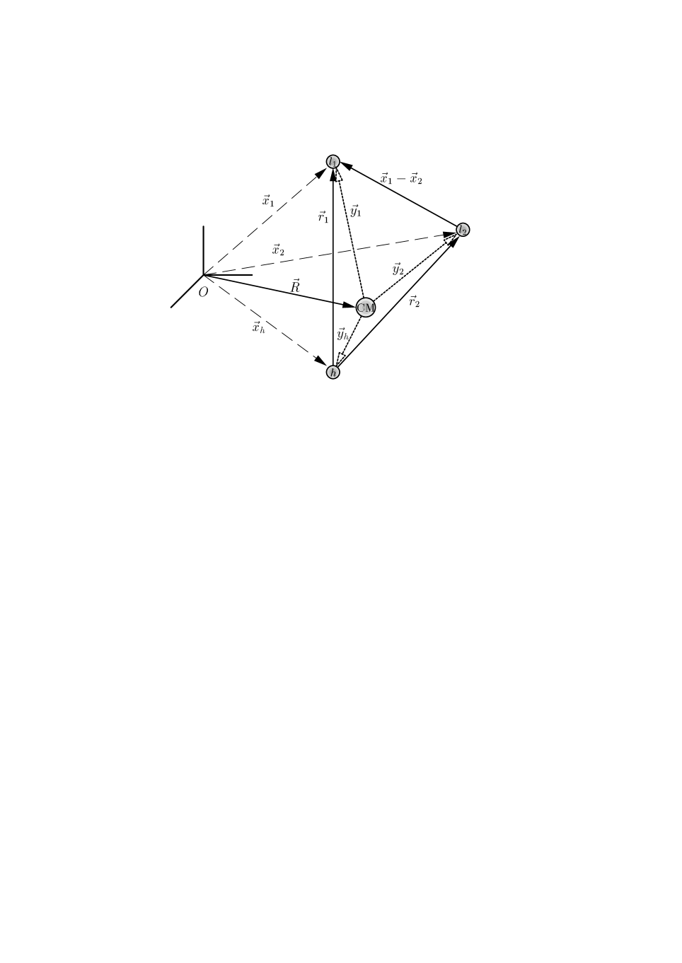
Figure 1: Definition of different coordinates used.

Working with the coordinates $\vec{R}$, $\vec{r}_{1}$ and $\vec{r}_{2}$ (see Fig. 1) we can separate the centre of mass motion and the Hamiltonian of the three quark system reads

$$H=-\frac{\vec{\nabla}_{\vec{R}}^{2}}{2M}+H^{\rm int}$$ (1)

$$H^{\rm int} = \sum_{i=1,2}\ H_{i}^{sp}+V_{l_{1}l_{2}}(\vec{r}_{1}-\vec{r}_{2},spin)$$

$$-\frac{\vec{\nabla}_{1}\cdot\vec{\nabla}_{2}}{m_{h}}+M$$

$$H_{i}^{sp} = -\frac{\vec{\nabla}_{i}^{2}}{2\mu_{i}}+V_{hl_{i}}(\vec{r}_{i},spin),\ \ i=1,2$$ (2)

The suffix $h$ stands for the heavy quark while $l_{1,2}$ refer to the light quarks. $M=(m_{l_{1}}+m_{l_{2}}+m_{h})$, $\mu_{i}=(1/m_{l_{i}}+1/m_{h})^{-1}$ and $\vec{\nabla}_{i}$ is the gradient with respect to $\vec{r}_{i}$. The internal wave function for a $\Lambda_{h}$ baryon ($h=b,c$) with spin projection $s$, isospin $I=0$ and total spin $S_{light}=0$ for the light degrees of freedom is given by

$$\left|\Lambda_{h};s\right> = \left\{\left|00\right>_{Iso.}\otimes\left|00\right>_{S_{light}}\right\}$$ (3)

$$\otimes\left|h;s\right>\psi(\vec{r}_{1},\vec{r}_{2})$$

The spatial wave function is obtained by using a simple variational ansatz

$$\psi(\vec{r}_{1},\vec{r}_{2}) = \varphi(r_{1},r_{2},r_{12})$$ (4)

$$= N\phi_{l_{1}}^{h}(r_{1})\phi_{l_{2}}^{h}(r_{2})F(r_{12})$$

where $N$ is a normalization factor and $F(r_{12})$ is a Jastrow-type correlation function

$$F(r_{12})=\sum_{j=1}^{4}a_{j}e^{-b_{j}^{2}(r_{12}+d_{j})^{2}}$$ (5)

being $a_{1}=1$ and $a_{i\neq 1},b_{i},d_{i}$ free parameters. $\phi_{l_{1}}^{h}(r_{1})$ and $\phi_{l_{2}}^{h}(r_{2})$ are essentially fixed by the s-wave ground state wave functions of the single particle Hamiltonians $H_{1,2}^{sp}$ for the relative motion of a light quark with respect to the heavy one. These wave functions are corrected at large distances where modifications coming from the presence of the other light quark are expected. This modification introduces two extra variational parameters.

Further details concerning wave functions, two-quark potentials used and the fixing of the parameters can be found in Ref. [10].

2.2 DECAY WIDTH

Neglecting lepton masses the differential cross section can be written as

$$\frac{d\,\Gamma}{d\omega} = \frac{G_{F}^{2}}{12\pi^{3}}\,|V_{cb}|^{2}\,M_{\Lambda_{c}}^{3}\,q^{2}\sqrt{\omega^{2}-1}$$ (6)

$$(-g^{\alpha\beta}+\frac{q^{\alpha}q^{\beta}}{q^{2}})\,H_{\alpha\beta}(q)$$

where $\omega$ is the product of four velocities $\omega=(p/M_{\Lambda_{b}})\cdot(p^{\prime}/M_{\Lambda_{c}})$, $q=p-p^{\prime}$ and $H_{\alpha\beta}(q)$ is the hadronic tensor defined as

$$H_{\alpha\beta}(q)$$

$$=\overline{\sum_{s,s^{\prime}}}\ \langle\Lambda_{c};s^{\prime},\vec{p}\,^{\prime}=-\vec{q}\,|(j_{cc})_{\alpha}(0)|\Lambda_{b};s,\vec{p}=\vec{0}\rangle$$

$$(\langle\Lambda_{c};s^{\prime},\vec{p}\,^{\prime}=-\vec{q}\,|(j_{cc})_{\beta}(0)|\Lambda_{b};s,\vec{p}=\vec{0}\rangle)^{*}$$ (7)

where $(j_{cc})^{\alpha}(0)=\bar{c}(0)\gamma^{\alpha}(1-\gamma_{5})b(0)$, and where $\vec{p}$ ($\vec{p}\,^{\prime}$) stands for the three-momentum of the $\Lambda_{b}$ ($\Lambda_{c}$) baryon. We have taken the $\Lambda_{b}$ baryon at rest and we have averaged (summed) over the spin $s$ ($s^{\prime}$) of the $\Lambda_{b}$ ($\Lambda_{c}$) baryon. Baryon states are normalized to “ E/M ”.

The matrix element of the weak charged current between hadronic states is parametrized in the usual way

$$\left<\Lambda_{c};s,\vec{p}\,^{\prime}|(j_{cc})^{\alpha}(0)|\Lambda_{b};s,\vec{p}\right>$$

$$\hskip 14.22636pt=\bar{u}_{\Lambda_{c}}^{(s^{\prime})}(\vec{p}\,^{\prime})\left[\ \gamma^{\alpha}(F_{1}-\gamma_{5}G_{1})\right.$$

$$\hskip 62.59596pt\left.+v^{\alpha}(F_{2}-\gamma_{5}G_{2})\right.$$

$$\hskip 62.59596pt\left.+v^{\prime\alpha}(F_{3}-\gamma_{5}G_{3})\ \right]u_{\Lambda_{b}}^{(s)}(\vec{p}\,)$$ (8)

where $v^{\alpha}=p/M_{\Lambda_{b}}$ ($v^{\prime\alpha}=p^{\prime}/M_{\Lambda_{c}}$) is the four- velocity of the $\Lambda_{b}$ ($\Lambda_{c}$) baryon.
In our nonrelativistic calculation we evaluate

$$\sqrt{\frac{M_{\Lambda_{b}}}{E_{\Lambda_{b}}(\vec{p})}}\sqrt{\frac{M_{\Lambda_{c}}}{E_{\Lambda_{c}}(\vec{p}\,^{\prime})}}\left<\Lambda_{c};s,\vec{p}\,^{\prime}|(j_{cc})^{\alpha}(0)|\Lambda_{b};s,\vec{p}\right>$$

which in momentum space is given by

$$\int d^{3}q_{1}d^{3}q_{2}d^{3}q_{h}d^{3}q_{h}^{\prime}\$$

$$\sqrt{\frac{m_{b}}{E_{b}(\vec{q}_{h})}}\sqrt{\frac{m_{c}}{E_{c}(\vec{q}\,^{\prime}_{h})}}[\bar{u}_{c}^{(s^{\prime})}(\vec{q}\,^{\prime}_{h})\gamma^{\mu}(1-\gamma_{5})u_{b}^{(s)}(\vec{q}_{h})]$$

$$\phi^{*(c)}(\vec{p}\,^{\prime};\vec{q}_{1},\vec{q}_{2},\vec{q}\,^{\prime}_{h})\ \phi^{(b)}(\vec{p};\vec{q}_{1},\vec{q}_{2},\vec{q}_{h})$$ (10)

with $\vec{p}\,^{\prime}=\vec{p}-\vec{q}$. The wave functions in momentum space appearing in the above equation are the Fourier transformed of those in coordinate space

$$\psi_{p}(\vec{x}_{1},\vec{x}_{2},\vec{x}_{h})=\frac{e^{i\vec{p}\cdot\vec{R}}}{(2\pi)^{\frac{3}{2}}}\psi(\vec{r}_{1},\vec{r}_{2})$$ (11)

with $\psi(\vec{r}_{1},\vec{r}_{2})$ described in the previous subsection.

The actual calculations are done in coordinate space. For that we need to expand the $b\to c$ transition operator in Eq.(2.2). In this expansion we shall keep up to terms in first order on $\vec{q}_{h}$. Being the $\Lambda_{b}$ baryon at rest, $\vec{q}_{h}$ is an internal momenta which is much smaller than any of the heavy quark masses. On the other hand the transferred momentum $\vec{q}$ can be large so that we do an exact expansion on $\vec{q}$.

3 PRELIMINARY RESULTS

Figure 2: Differential decay width

We present here the results obtained with the use of the wave functions that derive from the AL1 two-quark interaction potential (see Ref. [10] and references therein for details).

In Fig. 2 we show the differential decay width $d\Gamma(\omega)/d\omega$ in terms of $\omega$ (lower $x$-axis) and $q^{2}$ (upper $x$-axis).

The partially integrated value

$$\int_{1}^{1.2}d\omega\ \frac{d\Gamma(\omega)}{d\omega}=1.49\left|V_{cb}\right|^{2}\cdot 10^{13}s^{-1}$$ (12)

agrees nicely with a previous lattice calculation [3] which gives for this integral the value $1.4_{-4}^{+5}\left|V_{cb}\right|^{2}\cdot 10^{13}s^{-1}$. Our total width is given by

$$\int_{1}^{\omega_{max}}d\omega\frac{d\Gamma(\omega)}{d\omega}=3.41\left|V_{cb}\right|^{2}\cdot 10^{13}s^{-1}$$ (13)

Comparing to experimental data in Ref. [12] we can extract the value for the CKM matrix element

$$|V_{cb}|=0.047\pm 0.005$$ (14)

where we quote the error that derives from the experimental uncertainties. This value is in agreement with the recent determination by the DELPHI Collaboration [13] $|V_{cb}|=0.0414\pm 0.0012\pm 0.0021\pm 0.0018$, obtained from the analysis of the $\overline{B^{0}_{d}}\to D^{*+}l^{-}\bar{\nu}_{l}$ reaction.

Figure 3: Form factor $G_{1}(\omega)$ (solid line) and the sum $F_{1}(\omega)+F_{2}(\omega)+F_{3}(\omega)$ (dashed line). Data points are lattice calculations extrapolated down to the chiral limit as obtained in Ref. [3]

In Fig. 3 we show the results for the form factor $G_{1}(\omega)$ and the combination of form factors $F_{1}(\omega)+F_{2}(\omega)+F_{3}(\omega)$. Both quantities are protected by Luke’s theorem [14] from ${\cal O}(1/m_{h})$ corrections and are thus very close to the universal Isgur-Wise function [15]. As we see from the figure the two quantities are almost identical. We also show in the figure lattice results for the Isgur-Wise function obtained in Ref. [3] when the extrapolation to zero light quark masses is done. The value for the slope parameter $\rho^{2}$ defined as minus the slope at $\omega=1$ is given by

$$\hskip 42.67912pt\rho^{2}=0.98$$ (15)

and it is in good agreement with the central value obtained in the lattice determination which gives $\rho^{2}=1.1\pm 1.0$.

4 CONCLUSIONS

We have presented a calculation of the $\Lambda_{b}^{0}\to\Lambda_{c}^{+}l^{-}\bar{\nu}_{l}$ reaction within the context of NRCQM. We use manageable wave functions that were obtained in Ref. [10] using a simple variational ansatz based on HQS.

Our results for the partially integrated decay width and the Isgur-Wise function are in good agreement with previous lattice determinations. Comparison of our total decay width to experimental data allows us to obtain a value for $|V_{cb}|$ in agreement with a recent determination by the DELPHI Collaboration.

References

• [1] C. Albajar et al., Phys. Lett. B273, 540 (1991); G. Bari et al., Nuovo Cimento A10, 1787 (1991)
• [2] K. Hagiwara et al., Phys. Rev. D66, 010001 (2002).
• [3] K. C. Bowler et al., Phys. Rev. D57 6948 (1998).
• [4] M-Q Huang, J-P Lee, C. Liu and H.S. Song, Phys. Lett. B502 133 (2001).
• [5] F. Cardarelli and S. Simula, Nucl. Phys. A663 931 (2000); Phys. Rev. D60 074018 (1999); Phys. Lett. B421 295 (1998).
• [6] M. A. Ivanov, J. G. KΓΆrner, V. E. Lyubovitskij and A. G. Rusetsky, Phys. Rev. D59 074016 (1999).
• [7] J-P Lee, C. Liu and H.S. Song, Phys. Rev. D58 014013 (1998).
• [8] I. Dunietz, Phys. Rev. D58 094010 (1998).
• [9] N. Isgur and M. B. Wise, Phys. Lett.B232, 113 (1989); M. Neubert, Phys. Rep. 245 259 (1994); J. G. KΓΆrner, M. KrΓ€mer and D. Pirjol, Prog. Part. Nucl. Phys. 33, 787 (1994).
• [10] C. Albertus, J. E. Amaro, E. HernΓ‘ndez, J. Nieves. Nucl. Phys. A 740 (2004) 333-361
• [11] B. Silvestre-Brac, Few-Body Systems 20 (1996) 1.
• [12] S. Eidelman et al., Phys. Lett. B592, 1 (2004).
• [13] J. Abdallah et al. (DELPHI Collaboration), Eur. Phys. J. C33, 213 (2004)
• [14] M.E. Β Luke, Phys. Lett. B252, 447 (1990).
• [15] N.Β Isgur and M. B.Β Wise, Nucl. Phys. B348 (1991) 292.