The Abelianization of QCD Plasma Instabilities

Abstract

QCD plasma instabilities appear to play an important role in the equilibration of quark-gluon plasmas in heavy-ion collisions in the theoretical limit of weak coupling (i.e. asymptotically high energy). It is important to understand what non-linear physics eventually stops the exponential growth of unstable modes. It is already known that the initial growth of plasma instabilities in QCD closely parallels that in QED. However, once the unstable modes of the gauge-fields grow large enough for non-Abelian interactions between them to become important, one might guess that the dynamics of QCD plasma instabilities and QED plasma instabilities become very different. In this paper, we give suggestive arguments that non-Abelian self-interactions between the unstable modes are ineffective at stopping instability growth, and that the growing non-Abelian gauge fields become approximately Abelian after a certain stage in their growth. This in turn suggests that understanding the development of QCD plasma instabilities in the non-linear regime may have close parallels to similar processes in traditional plasma physics. We conjecture that the physics of collisionless plasma instabilities in SU(2) and SU(3) gauge theory becomes equivalent, respectively, to (i) traditional plasma physics, which is U(1) gauge theory, and (ii) plasma physics of U(1)$\times$U(1) gauge theory.

I Introduction

At high enough energy, heavy ion collisions are presumed to create a quark-gluon plasma in local equilibrium. The physics associated with the creation and equilibration of this plasma is rather complicated, involving many different physical processes playing important roles at different stages of the collision. It is theoretically useful to try to understand the collision in the formal limit of arbitrarily high energies, for which the running coupling constant $\alpha_{\rm s}$ is arbitrarily small due to asymptotic freedom. In this limit, it is believed that very early times are described by the saturation scenario gribov ; blaizot ; qiu ; larry ; krasnitz1 ; krasnitz2 , in which the non-equilibrium plasma starts out at early times $\tau_{0}\sim 1/Q_{\rm s}$ as a gas of gluons with (i) non-perturbatively large phase-space density $f\sim 1/\alpha_{\rm s}$ and (ii) momenta of order a scale $Q_{\rm s}$ known as the saturation scale. In the weak coupling limit $\alpha_{\rm s}(Q_{\rm s})\ll 1$, Baier, Mueller, Schiff and Son BMSS attempted to find the parametric dependence of the equilibration time $\tau_{\rm eq}$ on $\alpha_{\rm s}$ and found $\tau_{\rm eq}\sim\alpha^{-13/5}Q_{\rm s}^{-1}$. Their analysis is known as the bottom-up thermalization scenario, and the result arises from a complicated interplay of (i) the one-dimensional expansion of the plasma between the large, Lorentz-contracted, nuclear pancakes after the collision and (ii) a variety of individual collisional processes which relax the plasma toward equilibrium. However, collective processes are often more important in plasmas than individual collisions. In particular, Mrówczyński and others mrow0 ; mrow1 ; mrow2 ; mrow3 ; mrow&thoma ; randrup&mrow ; heinz_conf ; selikhov1 ; selikhov2 ; selikhov3 ; pavlenko have long suggested that plasma instabilities might play an important role in the equilibration of quark-gluon plasmas. Arnold, Lenaghan, and Moore alm showed that this is indeed the case for the bottom-up analysis. That means that the bottom-up scenario of Baier et al. needs to be completely reanalyzed. The theory of quark-gluon plasma equilibration in heavy-ion collisions is currently in the embarrassing state of not even knowing how the equilibration time depends on $\alpha_{\rm s}$ in the weak coupling limit — that is, not even the power $n$ is known in the parametric relation

$$\tau_{\rm eq}\sim\alpha^{-n}Q_{\rm s}^{-1}.$$ (1)

For ultra-relativistic, homogeneous, parity-invariant, collisionless plasmas, a long-wavelength magnetic instability known as the Weibel or filamentary instability generically arises whenever the momentum-distribution of charged particles in the plasma is anisotropic. A proof (and a more precise statement) may be found in Ref. alm . Reviews in the quark-gluon plasma literature of the physical origin of the instability may be found in Refs. mrow3 ; alm . The actual quark-gluon plasma in heavy-ion collisions is not collisionless, nor precisely homogeneous, but Ref. alm showed that the instabilities that plague the original bottom-up scenario are associated with small enough distance and time scales that collisions and inhomogeneity can be ignored. The analysis of such instabilities in the quark-gluon plasma literature has generally been restricted to linearized analysis, which treats the amplitude of the unstable long-wavelength magnetic field as perturbatively small. This is adequate for calculating the linear growth rate of the instability. In order to understand how instabilities affect equilibration, however, we need to know just how big the unstable long-wavelength magnetic field grows and what happens next. In particular, does the presence of this non-perturbatively large, long-wavelength field cause rapid isotropization and equilibration of the system? And what (parametrically) are the time scales involved? These questions cannot be answered by a linear analysis of the instability. In this paper, we will modestly focus on the very first question: How big does the instability grow? In answering this question, we will also learn important lessons concerning the qualitative nature of what happens to the unstable modes of the theory once they have grown large.

To investigate collective effects, it is both standard and convenient to describe the non-equilibrium quark-gluon plasma using kinetic theory in the form of Vlasov equations. We split the system into two parts: short wavelength (“hard”) momentum excitations which are described by a Boltzmann equation, and long-wavelength (“soft”) modes which are described by classical Maxwell equations. Hard excitations are treated as a collection of particles with phase-space density $f({\bm{p}},{\bm{x}},t)$. For an Abelian theory, the corresponding (collisionless) Boltzmann equation would be

$$\left[\partial_{t}+{\bm{v}}\cdot{\bm{\nabla}}_{\bm{x}}+g({\bm{E}}+{\bm{v}}\times{\bm{B}})\cdot{\bm{\nabla}}_{\bm{p}}\right]f=0,$$ (2)

where ${\bm{v}}$ is the velocity associated with ${\bm{p}}$, and ${\bm{E}}$ and ${\bm{B}}$ represent the fields of the long-wavelength modes (those not described by $f$). The corresponding Maxwell equations for the soft modes are

$$\partial_{\nu}F^{\mu\nu}=j^{\mu}=g\int_{\bm{p}}v^{\mu}f,$$ (3)

where there is an implicit sum over particle species on the right-hand side and $v^{\mu}\equiv(1,{\bm{v}})$. We use the $({-}{+}{+}{+})$ metric convention. One can generalize these fully non-linear Vlasov equations to non-Abelian plasmas. However, for the discussion in this paper, it is simpler to discuss the linearization of the equations in small fluctuations $\delta f({\bm{p}},{\bm{x}},t)$ of the distribution functions about some initial homogeneous distribution $f_{0}({\bm{p}})$. In this case,

$$(\partial_{t}+{\bm{v}}\cdot{\bm{\nabla}}_{\bm{x}})\,\delta f+g({\bm{E}}+{\bm{v}}\times{\bm{B}})\cdot{\bm{\nabla}}_{\bm{p}}f_{0}=0,$$ (4a)

$$\partial_{\nu}F^{\mu\nu}=j^{\mu}=g\int_{\bm{p}}v^{\mu}\,\delta f$$ (4b)

for the Abelian theory, assuming that $f_{0}$ carries no net charge or current. The non-Abelian generalization which describes the dynamics of long wave-length color electromagnetic fields is mrowKinetic ; HeinzKinetic ; BIkinetic

$$(D_{t}+{\bm{v}}\cdot{\bm{D}}_{\bm{x}})\,\delta f+g({\bm{E}}+{\bm{v}}\times{\bm{B}})\cdot{\bm{\nabla}}_{\bm{p}}f_{0}=0,$$ (5a)

$$D_{\nu}F^{\mu\nu}=j^{\mu}=cg\int_{\bm{p}}v^{\mu}\,\delta f,$$ (5b)

where $f_{0}$ is colorless and $\delta f$ takes values in the adjoint color representation. $D$ is the adjoint-representation covariant derivative, and $c$ is a constant that depends on the color representation of the hard particles. Note that we have linearized in $\delta f$ but not in the strength of the soft gauge field $A$. This is the usual starting point for kinetic theory discussions of hard thermal loops (HTLs) braaten&pisarski in non-Abelian plasmas, whether for isotropic or anisotropic $f_{0}$.

There are a number of conditions that must be met for collisionless Vlasov equations to give an accurate approximation to the underlying physical situation. The distance scales of interest must be (i) large compared to the deBroglie wavelength of the hard particles, so that hard particle propagation can be treated classically, and (ii) small compared to the mean free path for individual hard particle collisions, so that hard particle collisions may be ignored. The soft fields must be large enough that they can be treated as classical fields (i.e. the energy in each mode $k$ of interest should be large compared to the frequency $\omega_{k}$ of that mode). The last assumption will not be a problem for a growing unstable mode, once it has grown to significant size.

In the application to the thermalization of the quark-gluon plasma, the “hard particles” are the gluons with momenta of order the saturation scale $Q_{\rm s}$. The “soft” fields will refer to unstable modes of the gauge fields with much smaller momentum. (Note that hard and soft are relative terms, and, in much of the literature on saturation, the momentum scale $Q_{\rm s}$ would normally be thought of as a “soft” scale.) In order to keep the discussion of this paper somewhat general, we will henceforth refer to the hard momentum scale as $p_{\rm hard}$ or simply $p$ rather than $Q_{\rm s}$, and we will refer to the soft momentum scale as $k_{\rm soft}$ or simply $k$. We will assume $k_{\rm soft}\ll p_{\rm hard}$. This is the case for the plasma instabilities of the original bottom-up scenario at times $\tau\gg 1/Q_{\rm s}$ alm .

Though the precise value is not important to our discussion, the constant $c$ in (5b) is $c=2C_{\rm A}=6$ for hard gluons if $f$ represents the density of hard gluons per helicity and color state. $C_{\rm A}$ is the quadratic Casimir of the adjoint color representation, with $C_{\rm A}=N$ for SU($N$).

We can now lay out more precisely the basic question we will discuss in this paper. There are two distinct natural scales associated with the question of how big soft fields can grow before their effects can no longer be treated perturbatively in Eqs. (5). The first has to do with the Boltzmann equation (5a) and with when soft fields have a large effect on the trajectories of the hard particles—that is, with when the assumption $\delta f\ll f_{0}$ breaks down. Consider a soft magnetic field $B$. The hard particles will follow nearly straight-line (i.e. nearly free) trajectories if the Larmor radius $R\sim p_{\rm hard}/gB$ is large compared to the wavelength $\lambda\sim 1/k_{\rm soft}$ of the magnetic field. That is, the effects of the soft field on the hard particle trajectories are perturbative if

$$B\ll\frac{k_{\rm soft}\,p_{\rm hard}}{g}\,.$$ (6)

If one picks a “reasonable” gauge, where the gauge fields $A$ are relatively smooth and do not have variation on scales different from $k_{\rm soft}$, then $B\sim kA$, and this condition can be restated as

$$A\ll\frac{p_{\rm hard}}{g}\,.$$ (7)

In non-Abelian plasmas, however, we also have to think about the interaction of soft modes with each other. A quick way to estimate when these are important is to consider the covariant derivative $D=\partial-igA$ in the non-Abelian Maxwell equation (5b). When applied to the soft field strength $F$, we have $D\sim k_{\rm soft}-gA$. The $gA$ term can only be treated as a perturbation when $gA\ll k_{\rm soft}$, which is

$$A\ll\frac{k_{\rm soft}}{g}\,.$$ (8)

Which of these parametrically different scales determines how large the instabilities grow? Is it

$$A\sim\frac{p_{\rm hard}}{g}\,,$$ (9)

giving $B\sim kp/g$, or

$$A\sim\frac{k_{\rm soft}}{g}\ll\frac{p_{\rm hard}}{g}\,,$$ (10)

giving $B\sim k^{2}/g\ll kp/g$ ? That is, is the growth stopped by large effects on hard particle trajectories, or stopped earlier by non-Abelian interactions between the growing soft modes?

In the next section, we will briefly review the linearized theory of plasma instabilities. In section III, we then evaluate the effective potential for a certain class of unstable configurations and argue that, when non-linear interactions of the soft modes are considered, the instabilities will grow beyond the non-Abelian scale (10) by evolving toward Abelian configurations. In section IV, we check this assertion in a 1+1 dimensional toy model, which we simulate numerically. We find that the growing instabilities indeed evolve into gauge configurations living in the maximal Abelian sub-algebra of the gauge theory, which is U(1)$\times$U(1) for QCD. In section V, we briefly review what is known about the fate of plasma instabilities from studies of traditional plasmas, based on U(1) electromagnetism, once they grow large enough to saturate the Abelian bound (9). As an aside, in section VI we point out that there is a simple lower bound on the exponent $n$ in the parametric relation (1) for the equilibration time. Finally, we offer our conclusions in section VII. A number of topics briefly discussed in the main text are expanded upon in various appendices.

II Review of linear instability

One may formally solve the linearized Boltzmann equation (5a) for $\delta f$ and then insert the solution into Maxwell’s equation (5b) to obtain an effective equation of motion for the soft gauge fields:

$$D_{\nu}F^{\mu\nu}=-cg^{2}\int_{\bm{p}}v^{\mu}(D_{t}+{\bm{v}}\cdot{\bm{D}}_{\bm{x}}+\epsilon)^{-1}({\bm{E}}+{\bm{v}}\times{\bm{B}})\cdot{\bm{\nabla}}_{\bm{p}}f_{0},$$ (11)

where $\epsilon$ is a positive infinitesimal that selects the retarded solution. This equation simplifies enormously if one specializes to small gauge fields by linearizing in $A$. This limit has been analyzed by many authors, and the result is similar to that for an Abelian plasma of charged particles. Henceforth dropping the subscript on $f_{0}$, linearization yields

$$\partial_{\nu}F^{\mu\nu}\simeq-cg^{2}\int_{\bm{p}}v^{\mu}(\partial_{t}+{\bm{v}}\cdot{\bm{\nabla}}_{\bm{x}}+\epsilon)^{-1}({\bm{E}}+{\bm{v}}\times{\bm{B}})\cdot{\bm{\nabla}}_{\bm{p}}f.$$ (12)

Fourier transforming from $(t,{\bm{x}})$ to $K=(\omega,{\bm{k}})$, this can be put in the form

$$iK_{\nu}F^{\mu\nu}\simeq-\Pi^{\mu\nu}A_{\nu}$$ (13)

or equivalently

$$S^{\mu\nu}A_{\nu}=0,$$ (14)

where

$$S^{\mu\nu}(\omega,{\bm{k}})\equiv(-\omega^{2}+k^{2})g^{\mu\nu}-K^{\mu}K^{\nu}+\Pi^{\mu\nu}(\omega,{\bm{k}})$$ (15)

and

$$\Pi^{\mu\nu}(\omega,{\bm{k}})=cg^{2}\int_{\bm{p}}\frac{\partial f({\bm{p}})}{\partial p^{k}}\left[-v^{\mu}g^{k\nu}+\frac{v^{\mu}v^{\nu}k^{k}}{v\cdot K-i\epsilon}\right].$$ (16)

We will assume that $f({\bm{p}})$ is parity-invariant in what follows.

One can now investigate whether there are unstable solutions to (14), meaning solutions where $\omega$ has a positive imaginary part. Ref. alm uses continuity arguments to show that a sufficient condition for the existence of such an instability with a given wavenumber ${\bm{k}}$ is that the spatial part $S_{ij}$ of $S(\omega,{\bm{k}})$ have a negative eigenvalue at zero frequency. That is,

$$\varepsilon_{i}\bigl{[}k^{2}\delta_{ij}-k_{i}k_{j}+\Pi_{ij}(0,{\bm{k}})\bigr{]}\varepsilon_{j}<0$$ (17)

for some spatial polarization ${\bm{\varepsilon}}$ (which may be assumed transverse to ${\bm{k}}$ without loss of generality). This is a generalization of what’s known in plasma physics as the Penrose criterion. (See also the earlier discussion in Ref. mrow2 .) Roughly speaking, Ref. alm showed that this condition is satisfied for some ${\bm{k}}$ when $f({\bm{p}})$ is anisotropic. Note that a negative eigenvalue for $S_{ij}(0,{\bm{k}})$ requires a negative eigenvalue for the spatial self-energy $\Pi_{ij}(0,{\bm{k}})$.

Ref. alm also studied in detail a specific case relevant to the early stages of the original bottom-up scenario, where $f({\bm{p}})$ is axially symmetric and extremely anisotropic, with typical $p_{z}\ll p_{x},p_{y}$, as depicted schematically in Fig. 1a. Such a distribution has a flat pancake shape in ${\bm{p}}$ space. Qualitatively, the resulting set of soft, unstable modes arising from (14) was found to look like the region of ${\bm{k}}$ space depicted in Fig. 1b, which has a narrow cigar shape aligned along the $z$ axis. In this particular situation, typical unstable modes have ${\bm{k}}$’s which are almost parallel to the $z$ axis. Whether such extreme anisotropy will persist in the theory of quark-gluon plasma equilibration, once the effect of plasma instabilities are fully incorporated into the bottom-up scenario, is not yet known.

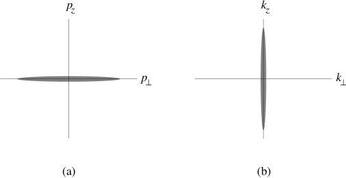
Figure 1: (a) Flat pancake shape of the distribution of hard particle momenta ${\bm{p}}$ in the early stages of the original bottom-up scenario. (b) Associated narrow cigar shape of the set of soft momenta ${\bm{k}}$ of unstable modes of the soft gauge fields. The scales in the two figures are not the same: $k_{\rm soft}\ll p_{\rm hard}$.

Before moving beyond the linearized effective theory of the soft gauge fields, it will be useful to note that the linearized equation of motion (14) can be associated with a corresponding effective action for the linearized theory:

$$S_{\rm eff}^{\rm(linearized)}=\int_{x}\left[-{\textstyle{\frac{1}{4}}}\,{\cal F}^{a}_{\mu\nu}{\cal F}^{a\mu\nu}-{\textstyle{\frac{1}{2}}}\,A^{a}_{\mu}\Pi^{\mu\nu}A^{a}_{\nu}\right],$$ (18)

where $x$ stands for $(t,{\bm{x}})$, and ${\cal F}_{\mu\nu}=\partial_{\mu}A_{\nu}-\partial_{\nu}A_{\mu}$ is the linear piece of the non-Abelian field strength $F_{\mu\nu}$. Note that the action is non-local because $\Pi^{\mu\nu}$, given by (16), is a non-local operator in $x$. In $A_{0}=0$ gauge, the action takes the form

$$S_{\rm eff}^{\rm(linearized)}=\int_{x}\left[{\textstyle{\frac{1}{2}}}|\partial_{t}{\bm{A}}|^{2}-{\textstyle{\frac{1}{2}}}|{\bm{\nabla}}\times{\bm{A}}|^{2}-{\textstyle{\frac{1}{2}}}\,A_{\mu}\Pi^{\mu\nu}A_{\nu}\right].$$ (19)

Studying the condition (17) for instability is equivalent to looking for unstable directions of the “potential energy” defined by considering the effective action (19) for static (that is, $\omega{=}0$) gauge fields:

$$V[{\bm{A}}] = \int_{\bm{x}}\left[{\textstyle{\frac{1}{2}}}|{\bm{\nabla}}\times{\bm{A}}|^{2}+{\textstyle{\frac{1}{2}}}A_{i}\,\Pi_{ij}(\omega{=}0)\,A_{j}\right]$$ (20)

$$= \int_{\bm{k}}{\textstyle{\frac{1}{2}}}\,A_{i}({\bm{k}})^{*}\bigl{[}k^{2}\delta_{ij}-k_{i}k_{j}+\Pi_{ij}(0,\hat{\bm{k}})\bigr{]}A_{j}({\bm{k}}).$$

In (20), we have written $\Pi_{ij}(0,\hat{\bm{k}})$ instead of $\Pi_{ij}(0,{\bm{k}})$. This is because the formula (16) for $\Pi(\omega,{\bm{k}})$ depends only on the direction $\hat{\bm{k}}$ (and not the magnitude) of ${\bm{k}}$ when $\omega=0$. We write $\Pi(0,\hat{\bm{k}})$ to emphasize this. In the limit $k\to 0$, the instability condition that $S_{ij}(0,{\bm{k}})$ have a negative eigenvalue is equivalent to $\Pi_{ij}(0,\hat{\bm{k}})$ having a negative eigenvalue.

Before continuing, we should mention some limitations of the effective potential. Note that, in $A_{0}{=}0$ gauge, the action for a free electromagnetic field $\int d^{4}x[{\textstyle{\frac{1}{2}}}|\partial_{t}{\bm{A}}|^{2}+{\textstyle{\frac{1}{2}}}|{\bm{B}}|^{2}]$ looks like a kinetic energy term ${\textstyle{\frac{1}{2}}}|\partial_{t}{\bm{A}}|^{2}$ which gives the electric energy, plus a potential energy term ${\textstyle{\frac{1}{2}}}|{\bm{B}}|^{2}$ which gives the magnetic energy. Generally, the effective potential in $A_{0}=0$ gauge represents magnetic potential energy, and electric effects are dynamical effects. As a result, one does not see electric effects such as Debye screening looking only at the effective potential (20). But one can use the effective potential as a way of understanding instabilities that manifest as negative eigenvalues of $\Pi_{ij}(0,\hat{\bm{k}})$.

III The effective potential

III.1 Hard particle effects

In order to investigate whether self-interactions of the soft gauge fields can stop the growth of the instabilities, we wish to analyze the effective potential energy without linearizing the effective theory in the gauge field $A^{\mu}$. Mrówczyński, Rebhan, and Strickland mrs have derived the effective action which gives the non-linear equation of motion (11). Their action for anisotropic $f$ is a generalization of the simple form of the HTL effective action derived by Braaten and Pisarski Sbp for isotropic $f$. It is given by

$$S_{\rm eff}=-\int_{x}{\textstyle{\frac{1}{4}}}{F^{a}}_{\mu\nu}F^{a\mu\nu}-cg^{2}\int_{x}\int_{\bm{p}}\frac{f({\bm{p}})}{p}\,{F^{a}}_{\alpha\mu}(x)\left(\frac{v^{\mu}v^{\nu}}{(v\cdot D)^{2}}\right)_{ab}{{F^{b}}_{\nu}}^{\alpha}(x).$$ (21)

To get the potential energy, we evaluate this action for static configurations ${\bm{A}}({\bm{x}})$ in $A_{0}=0$ gauge, as in the previous section. Even with these restrictions, the formula (21) remains a rather formal and complicated expression. However, it simplifies tremendously if we restrict attention to a certain sub-class of gauge field configurations inspired by Fig. 1. Because typical unstable ${\bm{k}}$’s in Fig. 1b have $k_{z}\gg k_{\perp}$, generic combinations of these modes will vary much more rapidly with $z$ than with $x$ or $y$. Let us therefore consider the extreme case of gauge field configurations that depend only on $z$:

$${\bm{A}}={\bm{A}}(z).$$ (22)

Making use of some observations by Blaizot and Iancu BIwaves , we show in Appendix A.1 that, for ${\bm{A}}={\bm{A}}(z)$, the effective action (21) reduces to the simple, local form

$$V[{\bm{A}}(z)] = \int_{\bm{x}}\left[{\textstyle{\frac{1}{4}}}F^{a}_{ij}F^{a}_{ij}+{\textstyle{\frac{1}{2}}}A^{a}_{i}\,\Pi_{ij}(0,\hat{\bm{e}}_{z})\,A^{a}_{j}\right]$$ (23)

$$= \int_{\bm{x}}\left[{\textstyle{\frac{1}{2}}}\,{\bm{B}}^{a}\cdot{\bm{B}}^{a}+{\textstyle{\frac{1}{2}}}A^{a}_{i}\,\Pi_{ij}(0,\hat{\bm{e}}_{z})\,A^{a}_{j}\right],$$

where $\Pi$ is the self-energy (16) of the linearized theory, and $\hat{\bm{e}}_{z}$ is the unit vector in the $z$ direction. ${\bm{B}}$ represents the full non-Abelian magnetic field. This is exactly the same as the result (20) of the linearized theory applied to configurations ${\bm{A}}={\bm{A}}(z)$ except that the quadratic $|{\bm{\nabla}}\times{\bm{A}}|^{2}$ term has been replaced by the full, non-Abelian $B^{2}$, which contains cubic and quartic interactions. The term ${\bm{A}}\Pi{\bm{A}}$ representing the effects of hard particles remains quadratic, however, even though we are no longer linearizing the theory in ${\bm{A}}$.

In field theory, one generally investigates questions of stability by studying the effective potential for low-momentum modes, taking $k\to 0$. If we take this limit in (23), we obtain the potential energy density

$${\cal V} = -{\textstyle{\frac{1}{4}}}\,g^{2}[A_{i},A_{j}]^{a}[A_{i},A_{j}]^{a}+{\textstyle{\frac{1}{2}}}A^{a}_{i}\,\Pi_{ij}(0,\hat{\bm{e}}_{z})\,A^{a}_{j},$$ (24)

$$= {\textstyle{\frac{1}{4}}}\,g^{2}f^{abc}f^{ade}A^{b}_{i}A^{c}_{j}A^{d}_{i}A^{e}_{j}+{\textstyle{\frac{1}{2}}}A^{a}_{i}\,\Pi_{ij}(0,\hat{\bm{e}}_{z})\,A^{a}_{j},$$

where $f^{abc}$ are the usual gauge-group structure constants. We can now investigate the topography of this potential in the space of $A^{a}_{i}$’s. We will assume that the hard particle distribution functions $f({\bm{p}})$ are axially symmetric about the $z$ axis and that $\Pi_{ij}(0,\hat{\bm{e}}_{z})$ has a negative eigenvalue, which is the case for oblate distributions like Fig. 1a. Using the transversality $K_{\mu}\,\Pi^{\mu\nu}(K)=0$ of the HTL self-energy (16), we can then write

$${\cal V}={\textstyle{\frac{1}{4}}}\,g^{2}f^{abc}f^{ade}A^{b}_{i}A^{c}_{j}A^{d}_{i}A^{e}_{j}-{\textstyle{\frac{1}{2}}}\,\mu^{2}(A^{a}_{x}A^{a}_{x}+A^{a}_{y}A^{a}_{y}),$$ (25)

where

$$\mu^{2}\equiv-\Pi_{xx}(0,\hat{\bm{e}}_{z})=-\Pi_{yy}(0,\hat{\bm{e}}_{z})>0.$$ (26)

In the linearized analysis, the unstable modes are those with $k<\mu$, and the typical unstable modes have $k_{\rm soft}\sim\mu$ (that is, $k<\mu$ but typically not $k\ll\mu$).

The potential (25) is unbounded below. Specifically, consider any “Abelian” configuration, by which we mean a gauge field where all the components $A_{i}$ of ${\bm{A}}$ commute. (For instance, this happens if the gauge field points in a single direction in adjoint color space, such as $A^{a}_{i}=A_{i}\delta^{a1}$.) Then the quartic term in the potential vanishes, leaving ${\cal V}=-{\textstyle{\frac{1}{2}}}\,\mu^{2}(A^{a}_{x}A^{a}_{x}+A^{a}_{y}A^{a}_{y})$, which clearly runs away to $-\infty$ as the magnitude of $A$ increases. Note that this picture can no longer be trusted when $A$ gets so large that the assumption $\delta f\ll f$ used to derive the effective action breaks down. That is, the runaway growth of Abelian configurations should stop when the size of $A$ is given by the scale $p_{\rm hard}/g$ of (9), as discussed in the introduction.

We can get a simple picture of the topography of ${\cal V}$ for non-Abelian configurations if we make some simplifying restrictions on ${\bm{A}}$. We will consider the case where both (i) ${\bm{A}}$ lies in an SU(2) subgroup of color SU(3) and (ii) $A_{z}=0$. With these assumptions, we show in Appendix A.2 that we can always make a combination of spatial and color rotations to put ${\bm{A}}(k\to 0)$ in the following form:

$$A_{i}^{a}=\phi_{1}\delta_{ix}\delta_{a1}+\phi_{2}\delta_{iy}\delta_{a2}.$$ (27)

The potential (25) is then

$${\cal V}(\phi_{1},\phi_{2})={\textstyle{\frac{1}{2}}}\,g^{2}\phi_{1}^{2}\phi_{2}^{2}-{\textstyle{\frac{1}{2}}}\,\mu^{2}(\phi_{1}^{2}+\phi_{2}^{2}).$$ (28)

This potential is depicted in Fig. 2. The Abelian configurations correspond to the $\phi_{1}$ axis ($\phi_{2}=0$) and the $\phi_{2}$ axis ($\phi_{1}=0$). One can see that there exist static non-Abelian solutions, indicated by the intersection points of the four straight lines in the figure. At these points, the amplitude of the gauge field is $A\sim\mu/g$. Recalling that unstable modes typically have $k_{\rm soft}\sim\mu$, this corresponds to the non-Abelian scale $A\sim k_{\rm soft}/g$ discussed in the introduction. However, these solutions are unstable to rolling down and subsequently growing in amplitude along one of the axis. The picture suggests that, if we start from $A$ near zero, the system might possibly at first roll toward one of these configurations with $A\sim k_{\rm soft}/g$, but its trajectory would eventually roll away and approximately “Abelianize,” growing along either the $\pm\phi_{1}$ or $\pm\phi_{2}$ axis until the effective action breaks down at $A\sim p_{\rm hard}/g$.

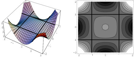
Figure 2: Two equivalent depictions of the potential $V(\phi_{1},\phi_{2})$ of (28). The $\phi_{1}$ and $\phi_{2}$ axis are in units of $\mu/g$, and the values of $V$ are in units of $\mu^{4}/g^{2}$. There is a local maximum with ${\cal V}=0$ at the origin. The four straight lines in the plots correspond to the equipotential $V=-\mu^{4}/2g^{2}$, and the four intersection points of those lines are saddle points corresponding to static, unstable, non-Abelian configurations.

We have been focusing on soft configurations ${\bm{A}}(z)$ in the arbitrarily long wavelength limit ${\bm{k}}\to 0$. In Appendix B, we show that the static, unstable, non-Abelian solutions discussed above have analogs with finite wavelength as well. These new solutions are also unstable and are merely a curiosity: they do not affect the current discussion.

III.2 Soft mode effects

So far, we have constructed the effective action and the effective potential by integrating out the effects of the hard particles. We have not yet, however, completely considered the effect that various soft field excitations with different ${\bm{k}}$’s can have on the instability. In order to illuminate the remaining issues, let us consider a very simple, warm-up toy model for the effective Lagrangian for the soft fields, which is a scalar field theory with the potential ${\cal V}(\phi_{1},\phi_{2})$ of (28):

$${\cal L}=-{\textstyle{\frac{1}{2}}}(\partial\phi_{1})^{2}-{\textstyle{\frac{1}{2}}}(\partial\phi_{2})^{2}-{\cal V}(\phi_{1},\phi_{2}).$$ (29)

As an example of a concern one might have about our previous discussion of instability, imagine that the soft sector were at some finite temperature $T\gg\mu$. What happens to our discussion when we account for the effects of interactions with modes with momenta of order $T$? It is well known that such interactions give a contribution of order $g^{2}T^{2}$ to the effective scalar mass-squared $m^{2}$. This effective $\Delta m^{2}$ is generated though diagrams such as Fig. 3a, which physically represent the forward scattering of particles off of the thermal bath, as in Fig. 3b. As a result,

$$-\mu^{2}\to-\mu^{2}+O(g^{2}T^{2})$$ (30)

in the effective potential (28). If $T$ were large enough, this would stabilize the potential near the origin and prevent runaway growth of the fields. This is the standard picture of high-temperature symmetry restoration in scalar field theories linde ; weinberg ; dolan&jackiw .

Figure 3: (a) 1-loop mass correction in finite-temperature diagrammatic perturbation theory. (b) Forward scattering off of a particle in the plasma.

Can anything similar happen in the problem of interest, where we consider an initial state that has very little energy in soft modes, but these modes subsequently grow because of the instability? In our toy scalar model, the answer is no. For the scalar theory, we give simple qualitative arguments (in any number of dimensions) in Appendix C. But a more straightforward way to verify our assertion is by explicit numerical simulation, which we discuss in the next section for 1+1 dimensions with a more sophisticated toy model than the scalar theory (29).

IV Numerical analysis of Abelianization in a toy model

There are several uses for performing a numerical simulation of a representative toy model of the physics we have been discussing. One is simply to verify our claim in Sec. III.2 that soft excitations produced during instability growth cannot stabilize the system from growth beyond the non-Abelian scale (10). Another is to better understand whether Abelianization is a global phenomena. We have suggested that the system, in searching to minimize its potential energy as the fields grow large, seeks configurations where commutators $[A_{i},A_{j}]$ are small, since these would otherwise contribute substantially to the non-Abelian magnetic field energy $B^{2}$. But is this a local statement or a global statement? Can one necessarily find a gauge where all $A_{i}({\bm{x}})$ commute with all $A_{j}({\bm{y}})$ for well-separated ${\bm{x}}$ and ${\bm{y}}$? That is, over what distance scale can one say that the non-Abelian gauge configurations are well approximated by purely Abelian gauge configurations, and does this distance scale grow with time? In this section, we will address these questions by numerical simulations of the real-time evolution of a 1+1 dimensional gauge theory.

IV.1 1+1 dimensional gauge theory toy model

Consider the full effective theory (21) of soft modes but restrict attention to gauge fields of the form

$$A_{\mu}=A_{\mu}(z,t).$$ (31)

This is similar to the restriction $A=A(z)$ of the last section, except that we now allow for time dependence. In addition, we will ignore time dependence in the second term of (21) so that it becomes the simple local ${\textstyle{\frac{1}{2}}}A_{i}^{a}\Pi_{ij}(0,\hat{\bm{e}}_{z})A^{a}_{j}$ of (25). This last approximation is not in general justified, which is why this will only be a toy model calculation, and we will discuss some of its deficiencies in Sec. IV.5. We hope it will qualitatively capture the physics of interest. In 1+1 dimensional language, $A_{0}$ and $A_{z}$ are the gauge fields, and $A_{x}$ and $A_{y}$ behave as adjoint-representation scalars. To emphasize this distinction, we will refer to $A_{x}$ and $A_{y}$ as $\phi_{x}$ and $\phi_{y}$ in what follows. The toy model Lagrangian is then

$${\cal L}={\textstyle{\frac{1}{2}}}E_{z}^{a}E_{z}^{a}+\sum_{\alpha=x,y}{\textstyle{\frac{1}{2}}}[(D_{0}\phi_{\alpha})^{a}(D_{0}\phi_{\alpha})^{a}-(D_{z}\phi_{\alpha})^{a}(D_{z}\phi_{\alpha})^{a}]-{\cal V}(\phi_{x},\phi_{y}),$$ (32)

where ${\cal V}(\phi_{x},\phi_{y})$ is the potential of (25). By writing $\phi=T^{a}\phi^{a}$, where $T^{a}$ are fundamental representation color generators with the usual normalization $\operatorname{tr}(T^{a}T^{b})={\textstyle{\frac{1}{2}}}\delta^{ab}$, we can also write this in the form

$${\cal L}=\operatorname{tr}(E_{z}^{2})+\operatorname{tr}[(D_{0}\phi_{x})^{2}-(D_{z}\phi_{x})^{2}]+\operatorname{tr}[(D_{0}\phi_{y})^{2}-(D_{z}\phi_{y})^{2}]-{\cal V}(\phi_{x},\phi_{y}),$$ (33)

$${\cal V}(\phi_{x},\phi_{y})=-\mu^{2}\operatorname{tr}(\phi_{x}^{2}+\phi_{y}^{2})+g^{2}\operatorname{tr}\left(\bigl{(}i[\phi_{x},\phi_{y}]\bigr{)}^{2}\right).$$ (34)

In $A_{0}=0$ gauge, the equations of motion are

$$\ddot{\phi}_{1} = (D_{z}^{2}+\mu^{2})\phi_{1}-g^{2}[\phi_{2},[\phi_{2},\phi_{1}]],$$ (35a)

$$\ddot{\phi}_{2} = (D_{z}^{2}+\mu^{2})\phi_{2}-g^{2}[\phi_{1},[\phi_{1},\phi_{2}]],$$ (35b)

$$\ddot{A}_{z} = ig[\phi_{x},D_{z}\phi_{x}]+ig[\phi_{y},D_{z}\phi_{y}],$$ (35c)

with $D_{z}\phi=\partial_{z}\phi-ig[A_{z},\phi]$. Gauss’s Law, which is a constraint equation preserved by the equations of motion, is

$$D_{z}\dot{A}_{z}=ig[\phi_{x},\dot{\phi}_{x}]+ig[\phi_{y},\dot{\phi}_{y}].$$ (36)

Classical evolution does not depend in any essential way on the value of $g$. One can remove $g$ by a simple rescaling of fields, $A_{\mu}\to A_{\mu}/g$ (including $A_{x}=\phi_{x}$ and $A_{y}=\phi_{y}$). This is equivalent to setting $g=1$ in the equations (35). Recall that the typical unstable modes have momenta of order $\mu$. It is therefore also natural to work in units where $\mu=1$, so that the condition (10) for when non-Abelian interactions between growing unstable modes first becomes important is simply $A_{\mu}\sim 1$. However, we will retain factors of $g$ and $\mu$ in what follows simply so that our notation and discussion is consistent with the conventions used earlier in this paper. Readers are encouraged to ignore these factors if so inclined, setting $g=1$ and $\mu=1$ in what follows.

Our goal will be to evolve the system (35) classically, starting from small, random initial conditions for the fields. Note that $A_{0}{=}0$ gauge is preserved by time-independent gauge transformations. In particular, in infinite volume, one can always find a time-independent gauge transformation to put the fields in axial gauge $A_{z}=0$ at a particular time $t_{1}$. We will use this freedom to choose our initial condition at $t=0$ to have $A_{z}=0$. We want tiny initial fluctuations in our soft fields to provide seeds for the soft-mode instabilities we wish to simulate. For $A_{x}=\phi_{x}$ and $A_{y}=\phi_{y}$, we choose their initial values to be zero and their initial time derivatives to be Gaussian random white noise with a very small amplitude $\Delta$. Gauss’s Law (36) then determines that $E_{z}=-\dot{A}_{z}$ must be $z$ independent at $t=0$. Since we are not interested in background electric fields, we take $E_{z}$ to be initially zero. In summary, our initial conditions (written in continuum notation) are

$$A_{z}(z,0)=\phi_{x}(z,0)=\phi_{y}(z,0)=0,\qquad E_{z}(z,0)=0,$$ (37a)

$$\bigl{\langle}\dot{\phi}^{a}_{\alpha}(z,0)\,\dot{\phi}^{b}_{\beta}(z^{\prime},0)\bigr{\rangle}=\frac{\Delta^{2}}{\mu}\,\delta^{ab}\delta_{\alpha\beta}\,\delta(z-z^{\prime}).$$ (37b)

In our simulations, we work on a 1-dimensional periodic spatial lattice with lattice spacing $a=0.05\,\mu^{-1}$ and length $L=250\,\mu^{-1}=5000\,a$. To evolve the system in time, we use a leapfrog time algorithm with time step $\epsilon=0.001\,\mu^{-1}$. Our algorithm very closely follows that of Refs. krasnitz ; ambjorn&krasnitz . Our discrete-time lattice evolution equations, along with the discretized version of our initial conditions, are given explicitly in Appendix D. We choose $\Delta$, which parametrizes the size of the initial fluctuations of $\dot{\phi}$, to be $\Delta=0.01\,(a\mu)^{1/2}\mu^{2}/g\simeq 0.002236\,\mu^{2}/g$. We evolve a single, representative, random initial field from the ensemble defined by (37b).

In addition to simulating the model for SU(3) gauge theory, we have also simulated it for SU(2) gauge theory. The color structure of SU(2) is slightly easier to discuss pedagogically because its maximal Abelian subgroup is U(1). If two adjoint fields commute in SU(2), they must be pointing in the same color direction. SU(3) is more complicated. For this reason, we start by discussing SU(2).

IV.2 Simulation Results: SU(2) gauge theory

Fig. 4 shows how the amplitude of the fields grows with time. Specifically, it shows the growth of the rms average

$$|\phi|_{\rm rms}\equiv\left[\int_{0}^{L}\frac{dz}{L}\>(\phi_{x}^{a}\phi_{x}^{a}+\phi_{y}^{a}\phi_{y}^{a})\right]^{1/2}=\left[\int_{0}^{L}\frac{dz}{L}\>2\operatorname{tr}(\phi_{x}^{2}+\phi_{y}^{2})\right]^{1/2}.$$ (38)

The figure also shows the volume average of the relative size of the local commutator $[\phi_{x},\phi_{y}]$ of the fields $A_{x}=\phi_{x}$ and $A_{y}=\phi_{y}$, as measured by

$$\overline{C}\equiv\int_{0}^{L}\frac{dz}{L}\>C(z),\qquad C\equiv\frac{\left\{\operatorname{tr}\left(\bigl{(}i[\phi_{x},\phi_{y}]\bigr{)}^{2}\right)\right\}^{1/2}}{\operatorname{tr}(\phi_{x}^{2}+\phi_{y}^{2})}\,.$$ (39)

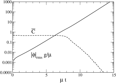
Figure 4: The average amplitude $|\phi|_{\rm rms}$ (solid) and the relative size $\overline{C}$ of commutators (dashed) as a function of time for gauge group SU(2).

As one can see, there is a stage of the instability growth, around $\phi\sim\mu/g$, where the original, random, non-Abelian fluctuations suddenly change character and $\phi_{x}$ and $\phi_{y}$ become, at least locally, aligned in the same color direction. We will analyze soon how global is this alignment.

Before continuing, we should note that quantities such as $\operatorname{tr}(A_{x}^{2}+A_{y}^{2})$ and $\operatorname{tr}([A_{x},A_{y}]^{2})$ are gauge-invariant under 1+1 dimensional gauge transformations, but they would not be be gauge-invariant in the original 3+1 dimensional theory under general 3+1 dimensional gauge transformations. This makes the construction of gauge-invariant observables easier in the 1+1 dimensional theory than in 3+1 dimensions. In particular, we can directly probe statements about the relative size of the commutator $[A_{x},A_{y}]$ without having to either (i) rely on the vague, qualitative statements like “in a reasonable gauge” which we used earlier in this paper, or (ii) construct more indirect observables, like commutators of magnetic fields. We shall take advantage of this feature of the 1+1 dimensional theory.

We have shown what happens to the relative size of $[\phi_{x},\phi_{y}]$. Readers may wonder about the other possible commutators of the basic fields of our model, $[A_{z},\phi_{x}]$ and $[A_{z},\phi_{y}]$. The value of $[A_{z},\phi_{\alpha}]$ at a particular moment is not physical because we can make it vanish everywhere by gauge transforming so that $A_{z}=0$ at that moment. We can think of fixing axial gauge at a particular time $t$ as the 1+1 dimensional analogue of a “smooth” gauge choice for that time slice.

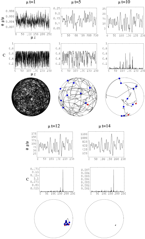
Figure 5: Snapshots in time of the evolution of SU(2) field configurations. Each column corresponds to a different time, labeled at the top: $\mu t=$ 1, 5, 10, 12, 14. For each time, the first row shows the total field strength (40), in units of $\mu/g$, as a function of $\mu z$. The second row shows the relative size $C$ of commutators as a function of $\mu z$. The third row shows the the color directions swept out in axial gauge as one varies $z$ from $0$ to $L$, as described in the text. The circles mark the points on these curves where $\mu z$ is a multiple of 50, and squares indicate the endpoints $z=0$ and $z=L$.

Snapshots of the field configurations are shown at five different times in Fig. 5. The first row shows the field strength

$$\Phi\equiv(\phi_{x}^{a}\phi_{x}^{a}+\phi_{y}^{a}\phi_{y}^{a})^{1/2}=\left[2\operatorname{tr}(\phi_{x}^{2}+\phi_{y}^{2})\right]^{1/2}$$ (40)

as a function of $z$. The second row shows the relative size $C$ of commutators, as defined in (39), again as a function of $z$. Note that the scales used in the graphs change with time.

We have learned that $\phi_{x}$ and $\phi_{y}$ point in the same color direction at late times. We would now like to address whether this direction “changes” with $z$. That is, is it possible to find a gauge where the fields all live in an Abelian sub-algebra of SU(2), e.g. all pointing in the $T^{3}$ direction:

$$A^{a}_{z}(z,t)=A_{z}(z,t)\,\delta^{a3},\qquad\phi^{a}_{\alpha}(z,t)=\phi_{\alpha}(z,t)\,\delta^{a3}.$$ (41)

A gauge-invariant way to compare the color directions of $\phi_{\alpha}(z)$ for different $z$ is to parallel transport all of the $\phi_{\alpha}(z)$ to some reference point $z_{0}$. We will pick $z_{0}=0$. Equivalently, one can simply gauge transform to $A_{z}{=}0$ gauge on the particular time slice of interest, in which case parallel transport is trivial and the color directions at different $z$ can be compared directly.

In SU(2), the color direction of an adjoint field $\phi^{a}$ can be represented as a unit 3-vector $(\phi^{1},\phi^{2},\phi^{3})/(\phi^{a}\phi^{a})^{1/2}$. It therefore lives on a 2-sphere $S^{2}$. However, the fields of an Abelian configuration (41) can take both positive and negative values, corresponding, for example, to color directions $(0,0,\pm 1)$. So, to test how much a given configuration deviates from being Abelian, we should not differentiate between a given color direction and its negative. The relevant color space is therefore $S^{2}$ with antipodal points identified ($S^{2}/Z_{2}$). The third row of Fig. 5 shows the (parallel transported) color directions swept out as $z$ varies from $0$ to $L$. The color direction is represented in the following way. Consider a color direction represented as a point on the unit sphere, as shown in Fig. 6. If it is in the lower hemisphere, use the identification of antipodal points to replace it by a point in the upper hemisphere. Then project the points in the upper hemisphere down to the plane passing through the equator. The plots in Fig. 5 show that plane. The dashed circles represent the equator, for which antipodal points are identified.

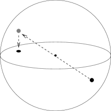
Figure 6: Projection of the space $S^{2}$ of SU(2) adjoint color directions into the plane, with the identification of antipodal points.

One can see from the color direction plots in Fig. 5 that the color directions globally align as $t$ gets large. At $\mu t=14$, the configuration is to very good approximation Abelian over the entire simulation volume. However, other aspects of the field remain uncorrelated. Fig. 7 shows the angle corresponding to the direction in the $xy$ plane of the essentially Abelian ${\bm{\phi}}\equiv(\phi_{x},\phi_{y})$ at $\mu t=14$, as a function of $z$. So, the SU(2) configurations at late times are homogeneous in color and look like a random superposition of unstable Abelian modes.

Figure 7: The angle in the $xy$ plane of the vector ${\bm{\phi}}\equiv(\phi_{x},\phi_{y})$, as a function of $\mu z$ at $\mu t=14$, for SU(2) simulations (taking ${\bm{\phi}}$ projected onto the color direction indicated in the last plot of Fig. 5).

IV.3 Abelianization Length: results for SU(2)

The adjoint color space of SU(3) is more complicated than that of SU(2). When we study SU(3) in the next section, we will not be able to make simple, visual plots of color direction as in Fig. 5. Also, the maximal Abelian subgroup of SU(2) is U(1), but the maximal Abelian subgroup of SU(3) is U(1)$\times$U(1). In SU(3), colors need not point in a single color direction in order to be Abelian. It will therefore be useful to replace our pictorial analysis by an appropriate correlation length that measures over what distance scales fields commute with each other. Consider the following correlation, which measures whether fields commute over a given distance $\xi$:

$$\chi_{\rm A}(\xi)\equiv\\ \frac{d_{\rm A}}{2C_{\rm A}}\int_{0}^{L}\frac{dz}{L}\frac{\operatorname{tr}\Bigl{\{}i\bigl{[}\phi_{\alpha}(z+\xi),\,{\cal U}(z+\xi,z)\,\phi_{\beta}(z)\bigr{]}\,i\bigl{[}\phi_{\alpha}(z+\xi),\,{\cal U}(z+\xi,z)\,\phi_{\beta}(z)\bigr{]}\Bigr{\}}}{\operatorname{tr}\left\{\phi_{\alpha}(z+\xi)\,\phi_{\alpha}(z+\xi)\right\}\,\operatorname{tr}\left\{\phi_{\beta}(z)\,\phi_{\beta}(z)\right\}}\,,$$ (42)

where ${\cal U}(z^{\prime},z)$ represents adjoint-representation parallel transport from $z$ to $z^{\prime}$. Specifically,

$${\cal U}(z^{\prime},z)\,\phi_{\beta}(z)=U(z^{\prime},z)\,\phi_{\beta}(z)\,\bigl{[}U(z^{\prime},z)\bigr{]}^{\dagger},$$ (43)

where $U(z^{\prime},z)$ is the fundamental-representation transporter

$$U(z^{\prime},z)={\cal P}\exp\left[ig\int_{z}^{z^{\prime}}dz^{\prime\prime}\>A_{z}(z^{\prime\prime})\right],$$ (44)

and ${\cal P}$ indicates path ordering (with $z^{\prime}$ on the left and $z$ on the right). Alternatively, one may transform to $A_{z}{=}0$ gauge and dispense with the parallel transporters. In (42), $d_{\rm A}$ and $C_{\rm A}$ are the dimension and quadratic Casimir of the adjoint color representation.

If commutators vanish locally, as we have seen they do for late times, then $\chi_{\rm A}(0)=0$. The correlation $\chi_{\rm A}$ has been normalized so that if the colors are completely uncorrelated over a distance $\xi$, then $\chi(\xi)=1$. We define the “Abelianization correlation length” $\xi_{\rm A}$ as the smallest distance $\xi$ for which $\chi_{\rm A}(\xi)\geq 0.5$. A plot of $\xi_{\rm A}$ vs. time for SU(2) is shown in Fig. 8. When $\xi_{\rm A}$ exceeds $L/2$ (indicated by the top of the plot), then the correlation does not drop below 0.5 anywhere on the lattice. One can see that this correlation length begins to grow rapidly at roughly the same time the relative size $\bar{C}$ of commutators begins to drop in Fig. 4.

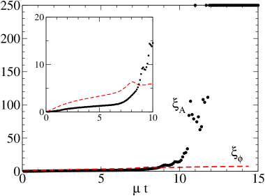
Figure 8: The solid lines and circles show the Abelianization correlation length $\xi_{\rm A}$ as a function of time, measured every $\delta t=0.1\,\mu^{-1}$. Individual points, rather than a continuous line, are shown simply because $\xi_{\rm A}$ jumps around quickly once it becomes a sizable fraction of the lattice. The dashed line shows the ordinary correlation length $\xi_{\phi}$. The topmost axis of the outer graph is $L/2$ and represents correlation lengths which exceed the size of our lattice. The inset provides an expanded view of the behavior for $\mu t<10$.

For comparison, we also plot in Fig. 8 a correlation length defined in terms of the full correlation (not just color) between the parallel-transported fields, defined by

$$\chi_{\phi}(\xi)\equiv\frac{\int_{0}^{L}\frac{dz}{L}\operatorname{tr}\left\{\phi_{\alpha}(z+\xi)\,{\cal U}(z+\xi,z)\,\phi_{\alpha}(z)\right\}}{\int_{0}^{L}\frac{dz}{L}\operatorname{tr}\left\{\phi_{\alpha}(z)\,\phi_{\alpha}(z)\right\}}\,.$$ (45)

This correlation is normalized so that $\chi(0)=1$, and $\chi(\xi)$ vanishes if the fields are uncorrelated over distance $\xi$. We define a correlation length $\xi_{\phi}$ by when this correlation first drops below 0.5. Note that this correlation length does not grow enormously like the Abelianization length $\xi_{\rm A}$ does.

IV.4 Simulation Results: SU(3) gauge theory

We are now ready to discuss simulation results for the QCD version of our 1+1 dimensional model. Simulation results for $|\phi|_{\rm rms}$, $\bar{C}$, $\xi_{\rm A}$ and $\xi_{\phi}$ for SU(3) are shown as a function of time in Figs. 9 and 10. The results are qualitatively similar to the SU(2) case, and we can draw the same conclusion from the rapid growth of $\xi_{\rm A}$: the configurations Abelianize as the field strength grows large compared to the natural non-Abelian scale $A\sim\mu/g$.

Plots of $\Phi$ and $C$ vs. $z$ are qualitatively similar to those of the SU(2) simulations shown in the first two rows of Fig. 5, and we will refrain from displaying them.

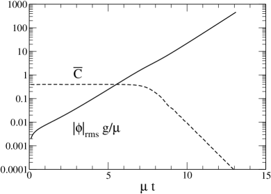
Figure 9: As Fig. 4 but for SU(3) gauge theory.

Figure 10: As Fig. 8 but for SU(3) gauge theory.

The Abelianization in SU(3) is slightly different than in SU(2) because the fields do not have to point in a single color direction. The maximal Abelian subgroup of SU(2) is U(1)$\times$U(1) and, after an appropriate gauge transformation, can be considered to be spanned by the diagonal generators

$$T^{3}=\frac{1}{2}\begin{pmatrix}1&&\\ &-1&\\ &&0\end{pmatrix},\qquad T^{8}=\frac{1}{\sqrt{12}}\begin{pmatrix}1&&\\ &1&\\ &&-2\end{pmatrix},$$ (46)

in the standard Gell-Mann representation. The analog of (41) for Abelian configurations is that they can be put in the form

$$A^{a}_{z}(z,t)=A^{3}_{z}(z,t)\,\delta^{a3}+A^{8}_{z}(z,t)\delta^{a8},\qquad\phi^{a}_{\alpha}(z,t)=\phi^{3}_{\alpha}(z,t)\,\delta^{a3}+\phi^{8}_{\alpha}(z,t)\,\delta^{a8}.$$ (47)

To investigate whether the late-time SU(3) configurations vary in color with $z$ within the maximal Abelian subgroup, we would like to plot the relative $T^{3}$ and $T^{8}$ components as a function of $z$. $T^{3}$ and $T^{8}$ are somewhat artificial choices, however, because they break the permutation symmetry of the U(1)$\times$U(1) subgroup, treating the first two colors of the fundamental representation differently from the third. In Fig. 11, we plot instead the gauge-invariant measures

$$\eta_{\alpha}(z)=\frac{3\sqrt{6}\,\det\phi_{\alpha}(z)}{\bigl{[}\operatorname{tr}(\phi_{\alpha}(z)\,\phi_{\alpha}(z))\bigr{]}^{3/2}}\qquad\qquad\mbox{(no sum on $\alpha$)}$$ (48)

vs. $z$. These parameters vary in magnitude $|\eta|$ between (i) zero, for color matrices with eigenvalues proportional to $(1,-1,0)$, like $T^{3}$ and its permutations, and (ii) 1, for color matrices with eigenvalues proportional to $(1,1,-2)$, like $T^{8}$ and its permutations. A plot of $\eta_{\alpha}(z)$ vs. $z$ is given for time $\mu t=13$. As one can see, the color direction within the maximal Abelian subgroup remains uncorrelated at this late time, even though the Abelianization correlation length is larger than the size of the lattice.

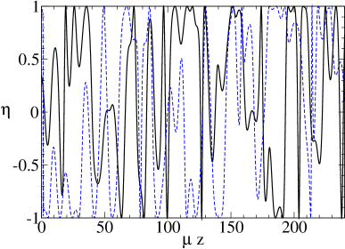
Figure 11: The parameters $\eta_{x}$ (solid) and $\eta_{y}$ (dashed) of (48) vs. $z$ for $\mu t=13$, showing the spatial variation of color within the maximal Abelian subgroup of SU(3).

IV.5 Differences between the toy model and the full effective theory

Before leaving our discussion of simulation results, we should mention one of the qualitative differences between our toy model (35) and the real theory of plasma instabilities. In constructing the toy model, we ignored time dependence in the second term of the effective action (21). Consider a linear analysis of instabilities around zero field. In our toy model, the growth rate of each mode with $k<\mu$ is given by

$$\gamma_{\rm toy}(k)=\sqrt{\mu^{2}-k^{2}},$$ (49)

which is easily derived by linearizing the equations of motion (35). Qualitatively, this growth rate has the form of the long-dashed line in Fig. 12 and is $\gamma_{\rm toy}=\mu$ at $k=0$. In the actual theory, where time dependence is not ignored, $\gamma(k)$ vanishes at $k=0$ mrow2 ; randrup&mrow ; alm ; strickland . For generic hard particle distributions, $\gamma(k)$ then has the qualitative form of the solid line in Fig. 12. The slow response of the system for small $k$ is related to Lenz’s Law: changing magnetic fields create electric fields, which induce currents to oppose the change. For the extremely anisotropic case of pancake distributions, such as shown in Fig. 1, instability growth is relatively slow compared to $\mu$ for all unstable $k$ alm . This is depicted by the short-dashed line in Fig. 12. We find it plausible that slow down of the growth rate will not affect the qualitative conclusions we have drawn: that energetics favors the development of Abelian configurations. However, this is something that should be checked in the future by simulations of the full theory. In particular, one might wonder whether the suppression of the growth of small $k$ modes in the full theory might affect the growth of the color correlation length to scales large compared to $\mu^{-1}$.

Figure 12: Qualitative behavior of linear growth rates of instabilities vs. momentum $k$ for (long-dashed) the toy model, (solid) actual QCD with a generic axi-symmetric hard particle distribution $f({\bm{p}})$, and (short-dashed) actual QCD with a pancake-shaped hard particle distribution.

V Fate of Abelian instabilities

If QCD plasma instabilities indeed Abelianize, then we may be able to learn qualitative lessons about their behavior from studies of traditional electromagnetic plasmas. Indeed, for SU(2) gauge theory, we have seen in our toy model that plasma instabilities grow into configurations of U(1) gauge theory. For QCD, the situation is a little more complicated: we get two copies of “electromagnetism” as U(1)$\times$U(1). Still, we may hope to gain some qualitative insight from what’s known about U(1) gauge theories. In this section, we will review a few relevant results from the traditional plasma literature.

Throughout this paper, we have focused on configurations which are approximately independent of $x$ and $y$, which arise naturally, for example, when the distribution of hard particles is pancake-shaped. One might wonder whether the dynamics continues to maintain the approximate independence of the configurations on $x$ and $y$ once the instabilities grow large enough that their effects on the hard particles become non-perturbative. Could the system settle down into oscillations about some non-linear $z$-dependent magnetic configurations, such as shown in Fig. 13a? Researchers have found examples of time-independent, non-perturbative wave solutions of the full (Abelian) non-linear collisionless Vlasov equations, such as the magnetic Bernstein-Greene-Kruskal (BGK) wave solutions discovered by Davidson et al. davidson&etal ; berger&davidson . However, one might guess that such solutions are inflicted with yet another type of plasma instability, known in different contexts as magnetic tear or reconnection instabilities.

Consider the magnetic field configuration depicted in Fig. 13a. By Ampere’s Law, a stable, time-independent solution of this form requires currents in the $x$ direction, also shown in the figure. Visualize the currents as being carried by wires. Two parallel wires with current in the same direction attract each other through magnetic interaction. There can then be an instability for the wires to dimerize—that is, clump together, as shown in Fig. 13b. The magnetic fields then change correspondingly, as indicated in the figure. In the context of collisionless plasma theory, an analytic analysis of this instability in a similar situation may be found in Ref. galeev . It has been observed in numerical simulations of non-relativistic plasmas by Califano et al. califano , which we will review in a moment. The interesting qualitative feature of the tear/reconnection instability is that it breaks the $xy$ translation invariance! The non-perturbative dynamics of fully grown plasma instabilities therefore has the potential to isotropize the system on relatively short time scales.

Figure 13: (a) Qualitative depiction of a non-linear magnetic BGK wave. The lines represent magnetic field lines. The points and crosses represent the net charged particle current, pointing either out of or into the page. (b) A magnetic tear or reconnection instability for the central region of figure (a).

Califano et al. study the case of a hard particle distribution corresponding to two similar, uniform, counter-streaming beams of electrons which have a tiny thermal spread of velocities around the beam velocities, as depicted in Fig. 14a. Additionally, rather than taking random initial conditions for the seed magnetic fields, they take initial conditions of the form

$${\bm{B}}=\mbox{(small)}\times\sin(k_{0}z)\,{\bm{e}}_{y}~{}~{}+~{}~{}\mbox{(much smaller random noise)}.$$ (50)

The first term seeds a single unstable mode that is $xy$ translation invariant and grows into something like the non-linear magnetic BGK mode discussed earlier. The second term is even smaller, and seeds the subsequent tear/reconnection instability of the magnetic BGK mode. They made the two terms different sizes because they wanted to clearly see a magnetic BGK mode and its subsequent demise, rather than having it all jumbled together. A qualitative depiction of the subsequent evolution, pieced together from Refs. davidson&etal ; califano , is shown in Fig. 14b. $T_{x}$, $T_{y}$, and $T_{z}$ are measures of the total kinetic energies along the $x$, $y$, and $z$ axis respectively, defined in terms of $mv_{x}^{2}$, $mv_{y}^{2}$, and $mv_{z}^{2}$. Initially, almost all of the electron kinetic energy is in the $x$ direction. Due to the Weibel instability, the first term of (50) then seeds the growth of a single, dominant unstable mode. The ${\bm{B}}$ field of that mode points in the $y$ direction and so can deflect the particles in the $xz$ plane but does not affect $v_{y}$. The growth of this instability eventually saturates in a nonlinear magnetic BGK-like state. Then, at late times, the second term of (50) grows due to the tear/reconnection instability. This instability drives the system toward isotropization of $T_{x}$, $T_{y}$, and $T_{z}$. Unfortunately, Califano et al.’s simulations end before one can see for sure whether there is complete isotropization.

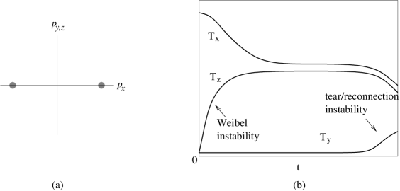
Figure 14: (a) A two-stream initial condition for $f({\bm{p}})$. (b) A qualitative picture of the resulting evolution of the initial magnetic seed field (50). The right half of figure (b) is a smoothed, qualitative sketch of the numerical results of Ref. califano . The left-hand side was not shown specifically in Ref. califano but is pieced together from statements in the text of that reference and from earlier simulations of the Weibel instability in Ref. davidson&etal .

One may wonder whether plasma instabilities always isotropize a collisionless plasma. Refs. honda ; taguchi ; semtoku ; lee&lampe numerically study parity-asymmetric initial conditions which do not isotropize. In particular, Honda et al. honda study the initial condition of a homogeneous beam of fast electrons in a plasma of slow electrons (and slower ions). As time evolves, they find that the Weibel instability causes clumping of the beam in the transverse direction. The resulting current filaments then attract each other magnetically (again just as two parallel wires carrying current in the same direction), and the filaments begin to merge, creating larger and larger filaments. Finally, there is only one filament left in their simulation volume, and the plasma stabilizes in this configuration. This final configuration is clearly anisotropic and corresponds to an equilibrium solution to the Vlasov equations originally found by Bennett in 1934 bennett , which we review for the ultra-relativistic case (where it is simpler) in Appendix E.

Because of the parity-noninvariance of the initial state, the simulations of Honda et al. could end up with a parity-noninvariant final state, described by the Bennett self-pinching filament. It is possible, in contrast, that generic parity-invariant initial conditions may lead to isotropization through collisionless processes, as suggested by the results of Califano et al.

VI Lower bound for the complete thermalization time

In the introduction, we pointed out the embarrassing fact that theory has so far been unable to determine even the power $n$ in the parametric relation $\tau_{\rm eq}\sim\alpha^{-n}Q_{\rm s}^{-1}$ for weak coupling, where $\tau_{\rm eq}$ is the local thermalization time. In this section, we point out that there is a simple lower bound on $n$. Consider the last part of thermalization, where the system is approximately but not fully equilibrated. At this point, we can use near-equilibrium results for the time scales associated with approach to equilibrium. Roughly, the characteristic time scale is then simply the equilibrium time scale for (i) large-angle deflections of a given particle’s direction, and (ii) number-changing processes such as hard gluon bremsstrahlung and $q\bar{q}$ creation or annihilation. Both of these processes have been considered in detail in the literature analyzing near-equilibrium transport processes, such as the calculation of the quark-gluon plasma shear viscosity shear ; shear1 ; shear2 . Parametrically, the time scale for both these types of processes is

$$\bar{t}\sim\frac{1}{\alpha_{\rm s}^{2}T}$$ (51)

up to a factor of $\ln(1/\alpha_{\rm s})$, which we will not bother to keep track of. Full local equilibration cannot happen any faster than this, and so

$$\tau_{\rm eq}\gtrsim\frac{1}{\alpha_{\rm s}^{2}T}\,.$$ (52)

If the system has fully equilibrated at time $\tau_{\rm eq}$ during the 1-dimensional expansion, then the energy density at that time,

$${\cal E}(\tau_{\rm eq})\sim\frac{{\cal E}(0)}{Q_{\rm s}\tau_{\rm eq}}\sim\frac{Q_{\rm s}^{4}}{\alpha_{\rm s}Q_{\rm s}\tau_{\rm eq}}\,,$$ (53)

must be $T^{4}$, so that

$$T\sim\frac{Q_{\rm s}}{(\alpha_{\rm s}Q_{\rm s}\tau_{\rm eq})^{1/4}}\,.$$ (54)

Combining (52) and (54), we obtain the lower bound

$$Q_{\rm s}\tau_{\rm eq}\gtrsim\alpha_{\rm s}^{-7/3}.$$ (55)

Note that the result $Q_{\rm s}\tau_{\rm eq}\sim\alpha_{\rm s}^{-13/5}$ of the original bottom-up scenario BMSS satisfies this bound. In that case, thermalization happened slower than the bound because the energy of the system got hung up for a time in hard modes, before it could equilibrate by cascading down into softer modes. The effects of plasma instabilities might speed up equilibration, and it is conceivable that the real answer could saturate the lower bound. Even if it does, one would still like to know all the various time scales associated with the different stages of equilibration, and what happens at each stage. The time scale for complete local equilibration might not be the most relevant time scale for understanding the physics of heavy ion collisions.

VII Conclusions

In this paper, we have examined the effect of non-Abelian self-interactions on growing plasma instabilities in an anisotropic non-Abelian plasma. By looking at the effective potential for $z$-dependent magnetic fields in the presence of an anisotropic distribution $f({\bm{p}})$ of hard particles, we have given suggestive arguments that non-Abelian interactions drive the growing instabilities to become Abelian once they grow large enough. Numerical simulations of a toy model 1+1 dimensional gauge theory also show this behavior. We conjecture that (i) the plasma instabilities of SU(2) gauge theory grow into those of traditional (relativistic) U(1) gauge theory, and (ii) the plasma instabilities of QCD grow into those of U(1)$\times$U(1) gauge theory, which is like traditional plasma theory but with two copies of electromagnetism. In the introduction, we asked what sets the scale for how large plasma instabilities grow. Our proposed answer is the Abelian one: the scale $A\sim p_{\rm soft}/g$ for hard particles to be affected non-perturbatively, rather than the scale $A\sim k_{\rm soft}/g$ for soft modes to have significant non-Abelian interactions.

Clearly, these conclusions need to be verified in 3+1 dimensional models, and with the full HTL effective action (21). In order to better understand the development of plasma instabilities once they are grown, full simulations of the full non-linear Vlasov equations are needed. Further simulations of traditional U(1) theories would provide useful information. Simulations of U(1)$\times$U(1) theories would be interesting as well. Of course, full simulations of non-linear SU(3) Vlasov equations would be even better. It is also possible that non-equilibrium QCD plasma physics could be studied in simulations of pure classical gauge theories on the lattice, in situations where there is a momentum scale separation so that excitation of some modes can be thought of as hard “particles” and others as soft fields.

Appendix A The effective potential for ${\bm{A}}={\bm{A}}(z)$

A.1 For ${\bm{A}}={\bm{A}}(z)$

In this appendix, we will derive the result (23) for the effective potential when ${\bm{A}}={\bm{A}}(z)$. We will begin, however, with a more general discussion. We find it advantageous to use a slightly different form of the effective action (21):

$$S_{\rm eff}=-\int_{x}{\textstyle{\frac{1}{4}}}{F^{a}}_{\mu\nu}F^{a\mu\nu}-cg^{2}\int_{x}\int_{\bm{p}}\frac{f}{p}\,{W^{a}}_{\alpha}W^{a\alpha},$$ (56a)

where

$$W_{\alpha}=W_{\alpha}(x,{\bm{v}})\equiv\frac{v^{\mu}}{v\cdot D}\,F_{\mu\alpha}(x).$$ (56b)

This form can be obtained from (21) by using the anti-symmetry of the operator ${\bm{v}}\cdot{\bm{D}}$ in $x$/color space to move one factor of $({\bm{v}}\cdot{\bm{D}})^{-1}$ from one $F$ to the other. Here and throughout this appendix, we will not bother keeping track of the $\epsilon$ prescriptions for retarded behavior. We note in passing that, in the isotropic case, Iancu iancuH has discussed a Hamiltonian formulation which is similar to (56).

Evaluating this action for static configurations ${\bm{A}}({\bm{x}})$ in $A_{0}=0$ gauge, we obtain

$$V_{\rm eff}=\int_{\bm{x}}{\textstyle{\frac{1}{4}}}F^{a}_{ij}F^{a}_{ij}+{\Delta V},$$ (57a)

where

$$\Delta V\equiv cg^{2}\int_{\bm{x}}\int_{\bm{p}}\frac{f}{p}\,W^{a}_{k}W^{a}_{k},$$ (57b)

and now

$$W_{k}=W_{k}({\bm{x}},{\bm{v}})=\frac{v_{i}}{{\bm{v}}\cdot{\bm{D}}}\,F_{ik}({\bm{x}}).$$ (57c)

Now we specialize to ${\bm{A}}={\bm{A}}(z)$. One can then make use of an identity noted by Blaizot and Iancu BIwaves , which is that

$$v\cdot D\left(A^{\alpha}-\frac{n^{\alpha}v\cdot A}{n\cdot v}\right)=v^{\nu}{F_{\nu}}^{\alpha}$$ (58)

if $A=A(n\cdot x)$ is only a function of $n\cdot x$, for some constant 4-vector $n$. This identity can be checked by explicitly expanding all the terms on both sides. Now apply $(v\cdot D)^{-1}$ to both sides of (58) to get

$$W^{\alpha}=A^{\alpha}-\frac{n^{\alpha}v\cdot A}{n\cdot v}.$$ (59)

In our case of ${\bm{A}}={\bm{A}}(z)$ with $A_{0}=0$, the identity is

$$W_{k}=A_{k}-\delta_{kz}\,\frac{{\bm{v}}\cdot{\bm{A}}}{v_{z}}.$$ (60)

Substituting into (57b), we then get that $\Delta V$ is quadratic in ${\bm{A}}(z)$. But that means that it must be the same as its expansion to quadratic order in ${\bm{A}}$, and so must be the same as the result in the linearized theory, giving

$$\Delta V{\bm{[}}{\bm{A}}(z){\bm{]}}=\int_{\bm{x}}{\textstyle{\frac{1}{2}}}\,A^{a}_{i}\Pi_{ij}A^{a}_{j}.$$ (61)

In ${\bm{k}}$ space, one may therefore write

$$\Delta V{\bm{[}}{\bm{A}}(z){\bm{]}}=\int_{\bm{k}}{\textstyle{\frac{1}{2}}}\,A^{a}_{i}({\bm{k}})^{*}\,\Pi_{ij}(0,\hat{\bm{k}})\,A^{a}_{j}({\bm{k}}).$$ (62)

Since the Fourier transform of ${\bm{A}}={\bm{A}}(z)$ has support only for ${\bm{k}}$’s proportional to $\hat{\bm{e}}_{z}$, we can replace $\Pi^{ij}(0,\hat{\bm{k}})$ by the matrix of constants $\Pi_{ij}(0,\hat{\bm{e}}_{z})$. The effective potential for ${\bm{A}}={\bm{A}}(z)$ is then local in ${\bm{x}}$ and may be written in the form (23).

A.2 For SU(2) with $k_{\perp}=0$, $k_{z}\to 0$ and $A_{z}=0$

In this section, we will simplify the potential ${\cal V}$ of (25) under the assumptions that (i) ${\bm{A}}$ lies in an SU(2) subgroup of color SU(3) and (ii) $A_{z}=0$. First, let’s consider the restriction to an SU(2) color subgroup. Then $f^{abc}$ can be replaced by $\epsilon^{abc}$, giving

$${\cal V}_{\rm SU(2)} = {\textstyle{\frac{1}{4}}}\,g^{2}\Bigl{[}(A^{b}_{i}A^{b}_{i})^{2}-A^{b}_{i}A^{c}_{j}A^{c}_{i}A^{b}_{j}\Bigl{]}-{\textstyle{\frac{1}{2}}}\,\mu^{2}(A^{a}_{x}A^{a}_{x}+A^{a}_{y}A^{a}_{y})$$ (63)

$$= {\textstyle{\frac{1}{4}}}\,g^{2}\Bigl{\{}[\operatorname{tr}({\cal A}^{\top}{\cal A})]^{2}-\operatorname{tr}[({\cal A}^{\top}{\cal A})^{2}]\Bigl{\}}-{\textstyle{\frac{1}{2}}}\,\mu^{2}\operatorname{tr}({\cal A}^{\top}P^{(xy)}{\cal A}),$$

where ${\cal A}$ is the $3\times 3$ matrix of $A_{ia}$,

$${\cal A}=\begin{pmatrix}A_{x}^{1}&A_{x}^{2}&A_{x}^{3}\\[2.0pt] A_{y}^{1}&A_{y}^{2}&A_{y}^{3}\\[2.0pt] A_{z}^{1}&A_{z}^{2}&A_{z}^{3}\end{pmatrix}.$$ (64)

$P^{(xy)}$ is the projection operator onto the $xy$ subspace of directions $i$,

$$P^{(xy)}=\begin{pmatrix}1&&\\ &1&\\ &&0\end{pmatrix}.$$ (65)

The potential is symmetric under (i) spatial rotations in the $xy$ plane, and (ii) color rotations. These symmetries can be summarized as

$${\cal A}\to R{\cal A}C^{\top},$$ (66)

where $C$ is a color rotation for the adjoint representation of SU(2), represented by any $3\times 3$ real, orthogonal matrix with $\det C=1$, and $R$ is a $3\times 3$ real, orthogonal matrix representing a rotation in the $xy$ plane. By a color transformation, we can assume without loss of generality that the matrix ${\cal A}$ is symmetric. Now make the remaining simplifying restriction that $A_{z}=0$. Then the symmetric ${\cal A}_{ia}$ is zero except for $i=x,y$ and $a=1,2$. We can then diagonalize the symmetric ${\cal A}$ in this $2\times 2$ subspace by a simultaneous space/color rotation of the form ${\cal A}\to R{\cal A}R^{\top}$. So, without further loss of generality, we may write

$${\cal A}=\begin{pmatrix}\phi_{1}&&\\ &\phi_{2}&\\ &&0\end{pmatrix}.$$ (67)

This gives (27).

Appendix B Unstable, non-Abelian, static waves

In this appendix, we show the existence of non-linear, non-Abelian, static wave solutions to the effective theory (56) of the soft modes. These solutions are classically unstable, however, to the Abelianization discussed in this paper. In the zero momentum limit ($k\to 0$), we will see that they correspond to the saddle points in Fig. 2.

The solutions are simple generalizations of propagating non-linear wave solutions found for equilibrium plasmas by Blaizot and Iancu BIwaves . We will look for solutions of the form $A=A(K\cdot x)$, for some 4-vector $K$. [We will shortly specialize to $K$ in the $z$ direction, so that $A=A(z)$.] As discussed in Appendix A, Blaizot and Iancu then showed that, in this case, the only effect of hard particles at leading order is to induce the HTL self-energy for the soft fields. The soft equation of motion is then

$$D_{\nu}F^{\mu\nu}=-\Pi^{\mu\nu}A_{\nu}.$$ (68)

Following one of the possibilities studied by Blaizot and Iancu, let’s focus on an SU(2) subgroup of the gauge group and further restrict attention to gauge fields of the form

$$A^{\mu}_{a}(n\cdot x)=\bigl{[}\epsilon^{\mu}_{(1)}\delta_{a1}+\epsilon^{\mu}_{(2)}\delta_{a2}\bigr{]}h(K\cdot x),$$ (69)

where $\epsilon^{\mu}_{(1,2)}$ is a basis of spatial polarizations orthogonal to ${\bm{k}}$. [This is essentially just (67) with $\phi_{1}=\phi_{2}=h(z)$, if one chooses $K$ along the $z$ axis.] The equation of motion (68) then becomes

$$(\omega^{2}-k^{2})h^{\prime\prime}+\Pi_{T}(\omega,{\bm{p}})\,h+g^{2}h^{3}=0,$$ (70)

where $h^{\prime\prime}$ indicates the second derivative of $h$ with respect to its argument $K\cdot x$.

Blaizot and Iancu considered eq. (70) for $\Pi_{T}$ positive, which is the situation for propagating modes in equilibrium situations. There are no non-trivial static solutions ($\omega=0$) in this case because $\Pi_{T}(0,{\bm{k}})=0$ in equilibrium. The difference in this paper is that we are interested in cases where $\Pi_{T}(0,{\bm{k}})$ can be negative because of the Weibel instability for anisotropic distributions. As a result, static solutions can exist to (70). Taking ${\bm{k}}$ to be in the $z$ direction, and writing $\Pi_{T}(0,{\bm{k}})=-\mu^{2}<0$, the static ($\omega=0$) case of (70) is

$$-\frac{d^{2}h}{dz^{2}}-\mu^{2}h+g^{2}h^{3}=0.$$ (71)

The solutions are

$$h(z)=\frac{\mu}{g}\left(\frac{2m}{1+m}\right)^{1/2}\operatorname{sn}\left(\frac{\mu z}{(1+m)^{1/2}}\,\Big{|}\,m\right),$$ (72)

for any $m$ with $0<m<1$. Here $\operatorname{sn}(u|m)$ is the Jacobi elliptic sine of argument $u$ and parameter $m$.

Now note that (71) is just the equation for static solutions of a scalar theory with potential $V(h)=-{\textstyle{\frac{1}{2}}}\mu^{2}h^{2}+{\textstyle{\frac{1}{4}}}g^{2}h^{4}$. This double-well potential is simply the potential of Fig. 2 along the diagonal $\phi_{1}=\phi_{2}$. The minima of $V(h)$ correspond to the saddle points of $V(\phi_{1},\phi_{2})$. In the ansatz (69), corresponding to $\phi_{1}=\phi_{2}$, we simply cannot see the unstable directions of the saddle point.

For $m\ll 1$ in (72), the solution has small-amplitude variations around $h=0$ as one changes $z$. As $m\to 1$, the solution becomes a regular array of far-separated kinks and anti-kinks, where the standard kink solution, centered on the origin, is $h(z)=(\mu/g)\,\tanh(\mu z/\sqrt{2})$. In this case, the kinks interpolate back and forth diagonally between the saddle points of Fig. 2, and in most of space, the field is nearly constant near one saddle point or the other. And so the constant-field instabilities discussed in the main text will locally afflict these solutions. For smaller $m$, where the kinks and anti-kinks begin to overlap, the potential energy can be further minimized by annihilating pairs of kinks and anti-kinks (that is, by dimerization): so again, these represent unstable solutions.

Appendix C Can soft excitations stop instability growth?

In this appendix, we give some qualitative arguments against the concerns raised in section III.2. We will argue that one should not expect effective masses generated by the soft sector to be able to prevent the growth of the system down along the valleys of the effective potential shown in Fig. 2. Because we discuss theories in different dimensions in this paper, we shall keep the spatial dimension $d$ general. For simplicity, we will restrict our discussion to the purely scalar theory of our warm-up toy model (29).

Imagine that the system starts with very tiny random magnetic noise, and the modes with $k\leq\mu$ then grow due to the instability. In a time of order $\mu^{-1}$ (neglecting factors of logarithms), the instabilities grow to the size of the soft non-perturbative scale $\mu/g$. Let’s start by supposing that the growth of the system did hang up at this scale. That is, suppose that the excitation of soft modes has built up to a point such that their contribution to the effective potential now cancels the destabilizing $-\mu^{2}$ quadratic coefficient contributed by the hard modes, so that, crudely speaking, the total effective potential at this time looks somewhat like Fig. 15 rather than Fig. 2 (which accounted only for the effects of the hard particles). The potential energy density released at this point would be of order $\mu^{4}/g^{2}$, which will also be the kinetic energy density of the soft field. At least initially, this energy would be in Fourier components with $k\sim\mu$ and with non-perturbatively large occupation numbers of order $1/g^{2}$. If the system were hung up, however, then it would quickly start to equilibrate by the strong non-perturbative self-interactions of these modes.

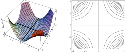
Figure 15: Like Fig. 2 but including a hypothetical contribution from soft modes that cancels the $-\mu^{2}A^{2}$ due to hard particles. This potential is zero along the axis. Qualitatively, the creation of just slightly more power in soft modes would cause it to curve up instead.

If the hung-up system were equilibrated, then the kinetic energy density $\mu^{4}/g^{2}$ would be $T^{d+1}$, giving $T\sim(\mu^{4}/g^{2})^{1/(d+1)}$. This gives $T\gg\mu$ for weakly-coupled theories $\mu^{d-3}g^{2}\ll 1$ in $d$ spatial dimensions. The energy would then be dominated by modes with momentum of order $T\gg\mu$. The drive toward thermalization would therefore push the energy of the system from modes with $k\sim\mu$ to modes with higher and higher momenta, until the system eventually thermalized (if it in fact remained hung up at $\phi\sim\mu/g$).

Let $\Lambda$ be the momentum scale that dominates the total kinetic energy at any time, which starts at order $\mu$. Due to the drive of the system toward thermalization, $\Lambda$ would grow several times in a time of order $\mu^{-1}$. Now consider a time when $\Lambda\gg\mu$. At this time, the kinetic energy density $\mu^{4}/g^{2}$, which must be of order $k^{2}\phi^{2}$, is distributed among modes with momentum $k\sim\Lambda$. So now $\phi\sim\mu^{2}/g\Lambda$. By mean field theory, the corresponding contribution to the squared effective mass is

$$(\Delta m^{2})_{\Lambda}\sim g^{2}\phi^{2}\sim\frac{\mu^{4}}{\Lambda^{2}}.$$ (73)

Were $\Lambda\sim\mu$, this might or might not be enough to compensate for the unstable $-\mu^{2}$ in the potential. However, since thermalization drives $\Lambda$ larger and larger, one will soon have $-\mu^{2}+(\Delta m^{2})_{\Lambda}<0$, and so instability to further growth, in a time scale of order $\mu^{-1}$.

There was an implicit assumption above that the momentum scale $\Lambda$ which dominates the kinetic energy is also the scale giving the dominant contribution to $\Delta m^{2}$. In low dimensions, this need not be the case. But even if all the energy were in modes $k\sim\mu$, corresponding to $\Lambda\sim\mu$ above, we have seen that the resulting $(\Delta m^{2})_{\mu}$ is order $\mu^{2}$. Once most of the energy has left modes $\mu\sim k$, then $(\Delta m^{2})_{\mu}$ will be $\ll\mu^{2}$. So neither $(\Delta m^{2})_{\mu}$ nor $(\Delta m^{2})_{\Lambda}$ will be enough to stop the continued growth of the instability.

Appendix D Lattice version of toy model

The lattice version of our 1+1 dimensional toy model, with spatial lattice spacing $a$, consists of the following elements. There are adjoint scalar fields $\phi_{x}$ and $\phi_{y}$, corresponding to $A_{x}$ and $A_{y}$, which live on the sites of the spatial lattice, represented as $N{\times}N$ traceless Hermitian matrices of su($N$). There are SU($N$) group elements $U$ living on the spatial links, corresponding to $\exp(iaA_{z})$ and represented as $N{\times}N$ unitary matrices. Then there are the conjugate momenta $\Pi_{x}$ and $\Pi_{y}$ (corresponding to $\dot{A}_{x}=-E_{x}$ and $\dot{A}_{y}=-E_{y}$) and $E$ (corresponding to $E_{z}$), which are all represented as $N{\times}N$ traceless Hermitian matrices living on the temporal links. In this appendix, we take $g=1$ and $\mu=1$. For time step $\epsilon$, our evolution equations are

$$\phi_{\alpha,s}(t+\epsilon) = \phi_{\alpha,s}(t)+\epsilon\,\Pi_{\alpha,s}(t+{\textstyle{\frac{1}{2}}}\epsilon),$$ (74)

$$U_{s+{\textstyle{\frac{1}{2}}}}(t+\epsilon) = U_{s+{\textstyle{\frac{1}{2}}}}(t)\>\exp\Bigl{(}-i\epsilon a\,E_{s}(t+{\textstyle{\frac{1}{2}}}\epsilon)\Bigr{)},$$ (75)

$$\Pi_{\alpha,s}(t+{\textstyle{\frac{1}{2}}}\epsilon) = \Pi_{\alpha,s}(t-{\textstyle{\frac{1}{2}}}\epsilon)+\epsilon\biggl{(}a^{-2}\Bigl{(}U_{s+{\textstyle{\frac{1}{2}}}}^{\dagger}\phi_{\alpha,s+1}U_{s+{\textstyle{\frac{1}{2}}}}-2\phi_{\alpha,s}+U_{s-{\textstyle{\frac{1}{2}}}}\phi_{\alpha,s-1}U_{s-{\textstyle{\frac{1}{2}}}}^{\dagger}\Bigr{)}$$ (76)

$$\hskip 90.00014pt+\mu^{2}\phi_{\alpha,s}-[\phi_{\bar{\alpha},s},[\phi_{\bar{\alpha},s},\phi_{\alpha,s}]]\biggl{)}_{t},$$

$$E_{s}(t+{\textstyle{\frac{1}{2}}}\epsilon) = E_{s}(t-{\textstyle{\frac{1}{2}}}\epsilon)-\frac{\epsilon}{a}\sum_{\alpha}i\big{[}\phi_{\alpha,s}\>,\>U_{s+{\textstyle{\frac{1}{2}}}}^{\dagger}\phi_{\alpha,s+1}U_{s+{\textstyle{\frac{1}{2}}}}\big{]}_{t},$$ (77)

where $s$ is an integer site index, $\alpha$ runs over $x$ and $y$, and $\bar{\alpha}$ denotes $y$ and $x$, respectively. Gauss’s Law is

$$a^{-1}\Bigl{(}E_{s}(t-{\textstyle{\frac{1}{2}}}\epsilon)-U_{s-{\textstyle{\frac{1}{2}}}}(t)\,E_{s-1}(t-{\textstyle{\frac{1}{2}}}\epsilon)\,U^{\dagger}_{s-{\textstyle{\frac{1}{2}}}}(t)\Bigr{)}+\sum_{\alpha}i\big{[}\phi_{\alpha,s}(t)\,,\,\Pi_{\alpha,s}(t-{\textstyle{\frac{1}{2}}}\epsilon)\big{]}=0.$$ (78)

The approximately conserved energy (which is exactly conserved for $\epsilon\to 0$) is

$${\cal E}=a\sum_{s}\biggl{[}\operatorname{tr}(E_{s}^{2})+\sum_{\alpha}\operatorname{tr}(\Pi_{\alpha,s}^{2})+\frac{1}{a^{2}}\sum_{\alpha}\operatorname{tr}\left(\Bigl{(}\phi_{\alpha,s}-U_{s-{\textstyle{\frac{1}{2}}}}\phi_{\alpha,s-1}U_{s-{\textstyle{\frac{1}{2}}}}^{\dagger}\Bigr{)}^{2}\right)\\ -\mu^{2}\operatorname{tr}(\phi_{x,s}^{2}+\phi_{y,s}^{2})+\operatorname{tr}\Bigl{(}\bigl{(}i[\phi_{x,s},\phi_{y,s}]\bigr{)}^{2}\Bigr{)}\biggr{]}.$$ (79)

In our simulations, the total energy of the system is very close to zero, because we start with very small initial fields. One can get a measure of how well energy is conserved in our simulations by comparing the change ${\cal E}(t)-{\cal E}(0)$ in the energy with time to the size of the potential energy $V(t)$ given by the last three terms of (79). By this measure, the simulations presented in this paper conserve energy at the level of 0.1%. We have checked that reducing the time step $\epsilon$ from the value $\epsilon=0.001$ used in our simulations (i) does not significantly change any of our simulation results, and (ii) indeed further improves energy conservation.

Our initial conditions (37) are

$$U_{s+{\textstyle{\frac{1}{2}}}}(0)=1,\qquad\phi_{\alpha,s}(0)=0,\qquad E_{s}(-{\textstyle{\frac{1}{2}}}\epsilon)=0,$$ (80)

$$\bigl{\langle}\Pi^{a}_{\alpha,s}(-{\textstyle{\frac{1}{2}}}\epsilon)\,\Pi^{b}_{\beta,s^{\prime}}(-{\textstyle{\frac{1}{2}}}\epsilon)\bigr{\rangle}=\frac{\Delta^{2}}{a}\,\delta^{ab}\delta_{\alpha\beta}\delta_{ss^{\prime}},$$ (81)

where $\langle\xi\xi\rangle=\Delta^{2}/a$ means choose $\xi$ to be a Gaussian random number centered on zero with standard deviation $\sigma=\Delta/a^{1/2}$. In our simulations, $\sigma=0.01$. The initial energy density $\rho_{0}$ is of order

$$\rho_{0}\sim\dot{\phi}^{2}\sim\sigma^{2}$$ (82)

and is dominated by stable UV modes.

We should check that our simulations will not run into a common difficulty in naively applying classical evolution equations to many problems, which is exemplified by the ultraviolet catastrophe of the classical blackbody spectrum. In thermal equilibrium, classical field theory (unlike its quantum counterpart), populates arbitrarily high momentum modes with real excitations. The interaction of these excitations with low-momentum modes of interest can cause arbitrarily large effects, in the continuum limit, on effective masses, damping rates, and other properties of the soft fields. (See, for example, Refs. alpha5 ; hotB .) Our simple white noise spectrum (81) populates arbitrarily high-momentum modes, so one might worry that there could be a similar problem here. As an example, let’s check the effective masses of soft modes due to interacting with UV modes of our lattice. Such masses arise from diagrams like Fig. 3. There are a number of ways to compute their scale. Treating the UV lattice modes with kinetic theory, for example,

$$\Delta m^{2}\sim g^{2}\int_{\bm{p}}\frac{f_{\bm{p}}}{p}\,.$$ (83)

where the integration is restricted to the UV modes whose effects are of interest. Previously in this paper, $f_{\bm{p}}$ has referred to hard particles. In this context, it refers instead to the UV modes of our classical continuum effective field theory of the “soft” modes. The energy density of these UV modes is $\rho\sim\int_{\bm{p}}E_{p}f_{\bm{p}}$. Parametrically, then,

$$\Delta m^{2}\sim\frac{g^{2}\rho}{p^{2}}\sim g^{2}\rho a^{2}.$$ (84)

The effects on the soft physics of interest will be small if $\Delta m^{2}\ll\mu^{2}$. Adopting our conventions $g=1$ and $\mu=1$, and using (82), this condition becomes

$$\sigma^{2}a^{2}\ll 1.$$ (85)

In our simulations, $\sigma^{2}a^{2}=2.5\times 10^{-7}$.

Appendix E Ultra-relativistic Bennett self-pinch

Traditional plasma physics is often complicated by the presence of multiple scales arising from the fact that ions are much heavier than electrons. Such complications vanish for electron-positron plasmas, or quark-gluon plasmas. In this appendix, we will summarize the self-pinching solutions to the collisionless Vlasov equations found by Bennett bennett in the simplifying situation where opposite charges have the same mass. This includes the ultra-relativistic limit, where particle masses are ignored. For simplicity of notation, we will focus on Abelian gauge theory. A class of self-pinching solutions for a plasma of charges $\pm e$ and mass $m$ is given by

$$f_{\pm}({\bm{x}},{\bm{p}})=\rho(r_{\perp})\,F_{\pm}({\bm{p}})$$ (86a)

in cylindrical coordinates $$(r_{\perp},\phi,z) F_{\pm}({\bm{p}})$$, where are boosted thermal distributions

$$F_{\pm}({\bm{p}})=\frac{\exp\left[-\gamma_{u}(E_{p}\mp up_{z})/T\right]}{\gamma_{u}Z_{m}},\qquad Z_{m}=\frac{m^{2}T}{2\pi^{2}}\,K_{2}\!\left(\frac{m}{T}\right)$$ (86b)

(with $$Z_{m}\to Z_{0}=T^{3}/\pi^{2} T\gg m \rho(r_{\perp})$$ in the ultra-relativistic limit ), and is the radial profile

$$\rho(r_{\perp})=\frac{\rho_{0}}{(1+b\rho_{0}r_{\perp}^{2})^{2}}\,,\qquad b=\frac{e^{2}\gamma_{u}u^{2}}{4T}\,.$$ (86c)

The constants $\rho_{0}$, $T$, and $u$ are arbitrary. One may check explicitly that (86) satisfies the time-independent collisionless Vlasov equations

$${\bm{v}}\cdot{\bm{\nabla}}f_{\pm}\pm e({\bm{E}}+{\bm{v}}\times{\bm{B}})\cdot{\bm{\nabla}}_{\bm{p}}f_{\pm}=0,$$ (87)

$${\bm{\nabla}}\cdot{\bm{E}}=e\int_{\bm{p}}(f_{+}-f_{-}),$$ (88)

$${\bm{\nabla}}\times{\bm{B}}=e\int_{\bm{p}}{\bm{v}}(f_{+}-f_{-}),$$ (89)

with ${\bm{E}}=0$ and

$${\bm{B}}=\frac{4Tb\rho_{0}r_{\perp}}{e\gamma_{u}u(1+b\rho_{0}r_{\perp}^{2})}\,{\bm{e}}_{\phi}.$$ (90)

This solution represents a finite-width beam of positively charged particles moving in the $+z$ direction and an exactly similar beam of negatively charged particles moving in the $-z$ direction. At their centers, each of these beams has density $\rho_{0}$ and looks like a thermal distribution with temperature $T$ boosted to a net beam velocity of magnitude $u$. The beam velocity $u$ can take any value $0<u<1$, even in the ultra-relativistic limit, since $u$ is the average velocity of particles in the beam.

References

- (1) L. V. Gribov, E. M. Levin and M. G. Ryskin, “Semihard processes in QCD,” Phys. Rept. 100, 1 (1983).
- (2) J. P. Blaizot and A. H. Mueller, “The early stage of ultrarelativistic heavy ion collisions,” Nucl. Phys. B 289, 847 (1987).
- (3) A. H. Mueller and J. W. Qiu, “Gluon recombination and shadowing at small values of x,” Nucl. Phys. B 268, 427 (1986).
- (4) L. D. McLerran and R. Venugopalan, “Computing quark and gluon distribution functions for very large nuclei,” Phys. Rev. D 49, 2233 (1994) [hep-ph/9309289]; “Green’s functions in the color field of a large nucleus,” Phys. Rev. D 50, 2225 (1994) [hep-ph/9402335].
- (5) A. Krasnitz and R. Venugopalan, “Non-perturbative computation of gluon mini-jet production in nuclear collisions at very high energies,” Nucl. Phys. B 557, 237 (1999) [hep-ph/9809433].
- (6) A. Krasnitz, Y. Nara and R. Venugopalan, “Coherent gluon production in very high energy heavy ion collisions,” Phys. Rev. Lett. 87, 192302 (2001) [hep-ph/0108092].
- (7) R. Baier, A. H. Mueller, D. Schiff and D. T. Son, “ ‘Bottom-up’ thermalization in heavy ion collisions,” Phys. Lett. B 502, 51 (2001) [hep-ph/0009237].
- (8) S. Mrówczyński, “Stream instabilities of the quark-gluon plasma,” Phys. Lett. B 214, 587 (1988).
- (9) S. Mrówczyński, “Plasma instability at the initial stage of ultrarelativistic heavy ion collisions,” Phys. Lett. B 314, 118 (1993).
- (10) S. Mrówczyński, “Color collective effects at the early stage of ultrarelativistic heavy ion collisions,” Phys. Rev. C 49, 2191 (1994).
- (11) S. Mrówczyński, “Color filamentation in ultrarelativistic heavy-ion collisions,” Phys. Lett. B 393, 26 (1997) [hep-ph/9606442].
- (12) S. Mrówczyński and M. H. Thoma, “Hard loop approach to anisotropic systems,” Phys. Rev. D 62, 036011 (2000) [hep-ph/0001164].
- (13) J. Randrup and S. Mrówczyński, “Chromodynamic Weibel instabilities in relativistic nuclear collisions,” Phys. Rev. C 68, 034909 (2003) [nucl-th/0303021].
- (14) U. W. Heinz, “Quark-qluon transport theory,” Nucl. Phys. A 418, 603C (1984).
- (15) Y. E. Pokrovsky and A. V. Selikhov, “Filamentation in a quark-gluon plasma,” JETP Lett. 47, 12 (1988) [Pisma Zh. Eksp. Teor. Fiz. 47, 11 (1988)].
- (16) Y. E. Pokrovsky and A. V. Selikhov, “Filamentation in quark plasma at finite temperatures,” Sov. J. Nucl. Phys. 52, 146 (1990) [Yad. Fiz. 52, 229 (1990)].
- (17) Y. E. Pokrovsky and A. V. Selikhov, “Filamentation in the quark-gluon plasma at finite temperatures,” Sov. J. Nucl. Phys. 52, 385 (1990) [Yad. Fiz. 52, 605 (1990)].
- (18) O. P. Pavlenko, “Filamentation instability of hot quark-gluon plasma with hard jet,” Sov. J. Nucl. Phys. 55, 1243 (1992) [Yad. Fiz. 55, 2239 (1992)].
- (19) P. Arnold, J. Lenaghan and G. D. Moore, “QCD plasma instabilities and bottom-up thermalization,” JHEP 08 (2003) 002 [hep-ph/0307325].
- (20) S. Mrowczynski, “Kinetic theory approach to quark-gluon plasma oscillations,” Phys. Rev. D 39, 1940 (1989).
- (21) H. T. Elze and U. W. Heinz, “Quark-gluon transport theory,” Phys. Rept. 183, 81 (1989).
- (22) J. P. Blaizot and E. Iancu, “Soft collective excitations in hot gauge theories,” Nucl. Phys. B 417, 608 (1994) [hep-ph/9306294].
- (23) P. F. Kelly, Q. Liu, C. Lucchesi and C. Manuel, “Deriving the hard thermal loops of QCD from classical transport theory,” Phys. Rev. Lett. 72, 3461 (1994) [hep-ph/9403403]; “Classical transport theory and hard thermal loops in the quark-gluon plasma,” Phys. Rev. D 50, 4209 (1994) [hep-ph/9406285].
- (24) E. Braaten and R. D. Pisarski, “Resummation and gauge invariance of the gluon damping rate in hot QCD,” Phys. Rev. Lett. 64, 1338 (1990).
- (25) P. Romatschke and M. Strickland, “Collective modes of an anisotropic quark gluon plasma,” Phys. Rev. D 68, 036004 (2003) [hep-ph/0304092].
- (26) S. Mrowczynski, A. Rebhan and M. Strickland, “Hard-loop effective action for anisotropic plasmas,” Phys. Rev. D 70, 025004 (2004) [hep-ph/0403256]; see hep-ph/0403256 for minor correction.
- (27) E. Braaten and R. D. Pisarski, “Simple effective Lagrangian for hard thermal loops,” Phys. Rev. D 45, 1827 (1992).
- (28) J. C. Taylor and S. M. H. Wong, “The effective action of hard thermal loops in QCD,” Nucl. Phys. B 346, 115 (1990).
- (29) J. P. Blaizot and E. Iancu, “Non-Abelian plane waves in the quark-gluon plasma,” Phys. Lett. B 326, 138 (1994) [hep-ph/9401323].
- (30) D. A. Kirzhnits and A. D. Linde, “Macroscopic consequences of the Weinberg model,” Phys. Lett. B 42, 471 (1972); “Symmetry Behavior in Gauge Theories,” Annals Phys. 101, 195 (1976).
- (31) S. Weinberg, “Gauge And global symmetries at high temperature,” Phys. Rev. D 9, 3357 (1974).
- (32) L. Dolan and R. Jackiw, “Symmetry behavior at finite temperature,” Phys. Rev. D 9, 3320 (1974).
- (33) A. Krasnitz, “Thermalization algorithms for classical gauge theories,” Nucl. Phys. B 455, 320 (1995) [hep-lat/9507025].
- (34) J. Ambjorn and A. Krasnitz, “The classical sphaleron transition rate exists and is equal to ,” Phys. Lett. B 362, 97 (1995) [hep-ph/9508202].
- (35) G. D. Moore, “Improved Hamiltonian for Minkowski Yang-Mills theory,” Nucl. Phys. B 480, 689 (1996) [hep-lat/9605001].
- (36) D. Y. Grigoriev, V. A. Rubakov and M. E. Shaposhnikov, “Sphaleron transitions at finite temperatures: numerical study in (1+1)-Dimensions,” Phys. Lett. B 216, 172 (1989).
- (37) J. Ambjorn, T. Askgaard, H. Porter and M. E. Shaposhnikov, “Sphaleron transitions and baryon asymmetry: a numerical real time analysis,” Nucl. Phys. B 353, 346 (1991).
- (38) R. C. Davidson, D. A. Hammer, U. Haber, and C. E. Wagner, “Nonlinear development of electromagnetic instabilities in anisotropic plasmas,” Phys. Fluids 15, 317 (1972).
- (39) R. L. Berger and R. C. Davidson, “Equilibrium and stability of large-amplitude magnetic Bernstein-Greene-Kruskal waves,” Phys. Fluids 15, 2327 (1972).
- (40) A. Galeev and R. Z. Sagdeev, “Current instabilities and anomalous reisistivity of plasma,” in Basic Plasma Physics II (vol. 2 of Handbook of Plasma Physics), eds. A.A. Galeev and R.N. Sudan (North-Holland, 1984).
- (41) T.-Y. B. Yang, J. Arons, A. B. Langdon, “Evolution of the Weibel instability in relativistically hot electron-positron beams,” Phys. Plasmas 1, 3059 (1994).
- (42) F. Califano, N. Attico, F. Pegoraro, G. Bertin, and S. V. Bulanov, “Fast formation of magnetic islands in a plasma in the presence of counterstreaming electrons,” Phys. Rev. Lett. 86, 5293 (2001).
- (43) M. Honda, J. Meyer-ter-Vehn, A. Pukhov, “Two-dimensional particle-in-cell simulation for magnetized transport of ultra-high relativistic currents in plasma,” Phys. Plasmas 7, 1302 (2000).
- (44) T. Taguchi, T. M. Antonsen, C. S. Liu, and K. Mima, “Structure formation and tearing of an MeV cylindrical electron beam in a laser-produced plasma,” Phys. Rev. Lett. 86, 5055 (2001).
- (45) Y. Semtoku, K. Mima, Z. M. Sheng, P. Kaw, K. Nishihara, K. Nishikawa, “Three-dimensional particle-in-cell simulations of energetic electron generation and transport with relativistic laser pulses in overdense plasmas,” Phys. Rev. E 65, 046408 (2002).
- (46) R. Lee and M. Lampe, “Electromagnetic instabilities, filamentation, and focusing of relativistic electron beams,” Phys. Rev. Lett. 31, 1390 (1973).
- (47) W. H. Bennett, “Magnetically self-focusing streams,” Phys. Rev. 45, 890 (1934).
- (48) P. Arnold, G. D. Moore and L. G. Yaffe, “Transport coefficients in high temperature gauge theories. II: Beyond leading log,” JHEP 05 (2003) 051 [hep-ph/0302165].
- (49) H. Hosoyo and K. Kajantie, “Transport coefficients of QCD matter,” Nucl. Phys. B 250, 666 (1985).
- (50) G. Baym, H. Monien, C. J. Pethick and D. G. Ravenhall, “Transverse interactions and transport in relativistic quark-gluon and electromagnetic plasmas,” Phys. Rev. Lett. 64, 1867 (1990).
- (51) E. Iancu, “Effective theory for real-time dynamics in hot gauge theories,” Phys. Lett. B 435, 152 (1998).
- (52) P. Arnold, D. Son and L. G. Yaffe, “The hot baryon violation rate is ,” Phys. Rev. D 55, 6264 (1997) [hep-ph/9609481].
- (53) P. Arnold, “Hot B violation, the lattice, and hard thermal loops,” Phys. Rev. D 55, 7781 (1997) [hep-ph/9701393].