Color Glass Condensate at the LHC:
hadron multiplicities in $pp$, $pA$ and $AA$ collisions

Abstract

We make quantitative predictions for the rapidity and centrality dependencies of hadron multiplicities in $AA$, $pA$ and $pp$ collisions at the LHC energies basing on the ideas of parton saturation in the Color Glass Condensate.

I Introduction

At high energies QCD is expected to enter the new phase : the Color Glass Condensate (CGC) which is characterized by strong coherent gluon fields leading to parton saturation GLR ; hdQCD ; MV ; BK ; JIMWLK . Previously, we have applied this approach KN ; KL ; KLN ; KLM ; KKT to describe the wealth of experimental data Brahms ; Phenix ; Phobos ; Star from RHIC. The LHC will allow to extend further the investigations of QCD in the regime of high parton density. This is because the new scale of the problem, the saturation momentum $Q_{s}$, will become so large ($Q^{2}_{s}\,\approx\,5-10\ {\rm GeV}^{2}$) that a separation of CGC physics from non-perturbative effects should become easier. The main objective of this paper is to give predictions for the global characteristics of the inelastic events in nucleus-nucleus, proton-nucleus and proton-proton collisions at LHC energies basing on the ideas of parton saturation in the Color Glass Condensate (CGC).

To understand better the differences implied by a higher energy of the LHC, let us start with the main assumptions of the approach we used to describe the data from RHIC:

1. At Bjorken $x\,\leq\,10^{-2}\,$ the inclusive production of partons (gluons and quarks) is driven by parton saturation in strong gluon fields as given by McLerran-Venugopalan model MV .

2. The region of $x\,\approx\,10^{-3}$ (accessible at forward rapidities at RHIC) is considered as the low $x$ region in which $\alpha_{S}\,\ln(1/x)\,\approx\,1$ so the quantum evolution becomes important; we assume that $\alpha_{S}\,\ll\,1$ to keep the calculation simple and transparent;

3. We assume that the interaction in the final state does not change significantly the multiplicities of partons resulting from the early stages of the process; this may be a consequence of local parton hadron duality, or of the entropy conservation. Therefore multiplicity measurements are extremely important for uncovering the reaction dynamics. However, we would like to state clearly that we do not claim that the interactions in the final state are unimportant. Rather, we consider the CGC as the initial condition for the subsequent evolution of the system, which can be described for example by means of hydrodynamics (such an approach has been followed in Refs. Eskola ; Hirano ).

Even a superficial glance at these three assumptions reveals that the conditions for the applicability of our approach at the LHC improve. Indeed, at LHC energies the value of $x$ will be two orders of magnitude lower than at RHIC. This makes the use of the well–developed methods of low $x$ physics MV1 ; BK ; JIMWLK ; LL ; IM ; KL ; MUSO better justified. At LHC energies we have a theoretical tool to deal with the high parton density QCD in the mean field approach ( so called Balitsky-Kovchegov non-linear equation BK ), or on a general basis of the JIMWLK equation JIMWLK ; even more general approaches may be possible (see for example the Iancu-Mueller factorization IM ; KLE ). However, despite a number of well developed approaches which could be applied at low $x$ we would like to warn that even the LHC energy is not high enough to apply any of the methods mentioned above without discussing possible ”pre-asymptotic” corrections to them.

Consider for example the determination of the value of the saturation momentum – the key scale in the CGC phase of QCD. As was noticed first in Ref. DIO the value of the saturation scale is affected by the next-to-leading order corrections to the BFKL kernel which were neglected in all of the discussed above approaches. Their numerical significance is so large that they cannot be neglected: if the next-to-leading order BFKL kernel is used, because of a large energy extrapolation interval to the LHC the value of $Q^{2}_{s}$ turns out to be 5 - 10 times smaller than if one uses the leading order kernel ( see detailed discussion in Ref. DUR ). However the good news is that the NLO corrections appear under theoretical control and we can take them into account.

The paper is organized as follows. In the second section we discuss the geometry of nucleus-nucleus and hadron-nucleus collisions and introduce the Glauber formalism we use. In the third section, we review the general formalism which we use to evaluate the multiplicities; we also discuss the influence of higher order corrections and the effects of the running coupling constant on the results. In the fourth section we list the parameters of our approach and justify the values we use; we then give a complete set of predictions for hadron multiplicities at the LHC energies in $Pb-Pb$, $p-Pb$, and $pp$ collisions, including the dependences on rapidity and centrality. We then summarize our results.

II The geometry of nucleus-nucleus and hadron-nucleus collisions and the Glauber approach

At high energies the paths of the colliding nucleons can be approximated by straight lines, since in a typical interaction $t/s\ll 1$ and the typical scattering angle is small. This is the most important approximation underlying the Glauber approach to nuclear interactions. Other approximations which simplify calculations but are in principle unnecessary are the smallness of the nucleon–nucleon interaction radius compared to the typical nuclear size, and the neglect of the real part of the $NN$ scattering amplitude. Many quantities characterizing the geometry of the collision can be readily computed in this approach; a complete set of the relevant formulae can be found e.g. in KNS and we will not reproduce all of them here.

It is customary and convenient to parameterize the centrality of the collision in terms of the ”number of participants” $N_{part}$ – the number of nucleons which underwent at least one inelastic collision. This number can be directly measured experimentally (at least in principle) by detecting in the forward rapidity region the number of ”spectator” nucleons $N_{spect}$ which did not take part in any inelastic collisions; obviously, for a nucleus with mass number $A$, $N_{part}=A-N_{spect}$.

The number of participating nucleons in a nucleus-A–nucleus-B interaction depends on the impact parameter $b$. In the eikonal approximation it can be evaluated as (see WNM ):

$$N_{part}^{AB}(b)=\int d^{2}s\,n_{part}^{AB}({\bf b},{\bf s}) = A\,\int d^{2}s\,T_{A}({\bf s})\left\{1-\left[1-\sigma_{in}\,T_{B}({\bf b}-{\bf s})\right]^{B}\right\}$$ (1)

$$+\,B\,\int d^{2}s\,T_{B}({\bf b}-{\bf s})\left\{1-\left[1-\sigma_{in}\,T_{A}({\bf s})\right]^{A}\right\}\,,$$

with the usual definition for the nuclear thickness function $T_{A}({\bf s})=\int_{-\infty}^{\infty}dz\rho_{A}(z,{\bf s})$, normalized as $\int d^{2}s\,T_{A}({\bf s})=1$; $\sigma_{in}$ is the proton-proton inelastic cross-section without diffractive component. For the LHC energies we assumed $\sigma_{in}=70$ mb (GLMSF ).

From Eq. (1) the definition of the local density of participants $n_{part}^{AB}({\bf b},{\bf s})$ is evident; we will define its average over the transverse plane as

$$\langle n_{part}^{AB}\rangle(b)=\frac{\int d^{2}s\,[n_{part}^{AB}({\bf b},{\bf s})]^{2}}{\int d^{2}s\,n_{part}^{AB}({\bf b},{\bf s})}~{}.$$ (2)

In the following we will need to use the average number of participants computed separately for nucleus-A and nucleus-B; it is given by

$$\langle n_{part,A}^{AB}\rangle(b)=\frac{\int d^{2}s\,n_{part,A}^{AB}({\bf b},{\bf s})\,n_{part}^{AB}({\bf b},{\bf s})}{\int d^{2}s\,n_{part}^{AB}({\bf b},{\bf s})}~{}.$$ (3)

Obviously, one has for their sum

$$\langle n_{part,A}^{AB}\rangle(b)+\langle n_{part,B}^{AB}\rangle(b)=\langle n_{part}^{AB}\rangle(b)$$

where $\langle n_{part,A}^{AB}\rangle(b)$ and $\langle n_{part,B}^{AB}\rangle(b)$ are the integrands of the first term and second term in the r.h.s of Eq. (1) respectively.

In table 1 we give the number of participants and their density (respectively Eqs. (1) and (2)) for Pb-Pb collisions at LHC.

$\begin{array}[]{c}b\\ ({\mathrm{fm}})\end{array}$	$N_{part}^{AB}$	$\begin{array}[]{c}n_{part}^{AB}\\ ({\mathrm{fm}}^{-2})\end{array}$	$\begin{array}[]{c}b\\ ({\mathrm{fm}})\end{array}$	$N_{part}^{AB}$	$\begin{array}[]{c}n_{part}^{AB}\\ ({\mathrm{fm}}^{-2})\end{array}$
0.00	406.9	2.98	8.00	166.8	2.21
1.00	402.4	2.97	9.00	127.5	1.97
2.00	387.8	2.93	10.00	91.9	1.69
3.00	363.2	2.88	11.00	61.1	1.35
4.00	330.3	2.80	12.00	36.2	0.98
5.00	291.9	2.70	13.00	18.3	0.59
6.00	250.6	2.57	14.00	7.5	0.27
7.00	208.3	2.41	15.00	2.5	0.09

Table 1: Mean number of participants and their average density in Pb-Pb collisions at LHC as a function of $b$

The corresponding formulae for the proton–nucleus $pA$ interaction can be deduced by setting $B=1$ and using a delta-function for the proton thickness function (in the point-like approximation for the size of the proton). We get from Eq. (1):

$$N_{part}^{pA}(b)=A\,\sigma_{in}\,T_{A}(b)+\left\{1-\left[1-\sigma_{in}\,T_{A}(b)\right]^{A}\right\}\,=A\,\sigma_{in}\,T_{A}(b)+\left\{1-P_{0}^{pA}(b)\right\}.$$ (4)

In the previous formula the function $P_{0}^{pA}(b)$ is the probability of no interaction in a p-A collision at impact parameter $b$; the integration of $[1-P_{0}^{pA}(b)]$ over $b$ gives the inelastic proton-nucleus cross section $\sigma_{pA}$.

The average number of participants in a p-A collision can be obtained as:

$$\langle N_{part}^{pA}\rangle=\frac{\int\mathrm{d\,}^{2}b\,N_{part}^{pA}(b)}{\int\mathrm{d\,}^{2}b\,[1-P_{0}(b)]}=A\,\frac{\sigma_{in}}{\sigma_{pA}}+1;$$ (5)

the first term in the r.h.s. gives the mean number of participants $\langle N_{part,A}^{pA}\rangle$ in the nucleus. As in the case of nucleus-nucleus collision, we will need to compute the density of participants in nucleus A, defined as:

$$\langle n_{part,A}^{pA}\rangle=\frac{\langle N_{part,A}^{pA}\rangle}{\sigma_{in}}=\frac{A}{\sigma_{pA}}.$$ (6)

In practice, the information about the impact parameter dependence is extracted by analyzing the data in various centrality bins. The physical observable most frequently used to estimate the centrality of the collision is the multiplicity of charged particles $N_{ch}$. We will assume that the average value of $N_{ch}$ produced in a collision at impact parameter $b$ is determined by the number of participating nucleons $N_{part}(b)$. The actual multiplicity will fluctuate around its mean value according to:

$${\mathcal{P}}(N_{ch},\langle N_{ch}(b)\rangle)=\frac{1}{\sqrt{2\pi a\langle N_{ch}(b)\rangle}}\,C(\langle N_{ch}(b)\rangle)\,\mathrm{exp}\left\{-\frac{[N_{ch}-\langle N_{ch}(b)\rangle]^{2}}{2a\langle N_{ch}(b)\rangle}\right\},$$ (7)

where the factor $C(N)\equiv 2/[1+erf(\sqrt{N/2a})]$ is introduced to ensure that the fluctuation function ${\mathcal{P}}(N_{ch},N)$ satisfies $\int_{0}^{\infty}dN_{ch}{\mathcal{P}}(N_{ch},N)=1$. The numerical value of $C(N)$ is 1 with very good accuracy for almost all cases of practical interest (it can exceed 1 for very peripheral collisions, where the number of participants and consequently $N_{ch}$ is small: in such a case it is important to include the factor $C(N)$ to have a correct normalization).

The parameter $a$ gives the width of the fluctuations: its value is dependent on the experimental apparatus, therefore it is not possible for us to predict its value for the LHC experiments. For the experiments at SPS and RHIC the value of $a$ varies from 0.5 to 1.5-2. We will assume $a=0.5$ in the following; uncertainty in this parameter can affect the centrality dependence of our results. In the case of $PbPb$ collisions, we estimate the resulting uncertainty in the density of participants (and thus in the saturation scale, see below) to be about $5\%$; in the case of $pPb$ collisions, this uncertainty can reach $10\div 15\%$ for peripheral collisions.

We will also assume the proportionality between $N_{ch}$ and $N_{part}$ when computing the differential inelastic cross section; this proportionality is not exact, but the shape of minimum bias distribution of events which is normally used to fix the parameter $a$ (and the proportionality constant between $N_{ch}$ and $N_{part}$) has been found insensitive to this assumption (see KN ).

The minimum bias differential cross section can be obtained as ($N(b)\equiv qN_{part}(b)$, where $q$ is a constant):

$$\frac{d\sigma_{mb}}{dN_{ch}}=\int d^{2}b\,{\mathcal{P}}(N_{ch},N(b))\,\left[1-P_{0}(b)\right];$$ (8)

here $P_{0}(b)$ is the probability of no interaction at the impact parameter $b$: for a nucleus-nucleus collision $P_{0}(b)=[1-\sigma_{in}T_{AB}(b)]^{AB}$ where $T_{AB}$ is the overlap function : $T_{AB}(b)=\int d^{2}s\,T_{A}(s)T_{B}({\bf b}-{\bf s})$; in the case of B=1, $P_{0}(b)$ reduces to $P_{0}^{pA}(b)$ defined above. In the following, all of the formulae will refer to A-B collisions; with obvious modifications they are valid also in the p-A case.

The total nucleus-nucleus cross section is then obtained by integrating Eq. (8) over $dN_{ch}$:

$$\sigma_{AB}=\int dN_{ch}\,\frac{d\sigma_{mb}}{dN_{ch}}=\int d^{2}b\,\left[1-P_{0}(b)\right].$$ (9)

The mean value of any physical observable ${\mathcal{O}}$ (given in terms of the impact parameter $b$) can be computed as:

$$\langle{\mathcal{O}}\rangle=\frac{1}{\sigma_{AB}}\int dN_{ch}\,\frac{d\sigma_{mb}}{dN_{ch}}\,{\mathcal{O}}(b)$$ (10)

To obtain the corresponding average for a given centrality cut we have to limit the integrations in the previous formula in the appropriate way, for instance the expression:

$$\left.\langle{\mathcal{O}}\rangle\vphantom{\frac{1}{1}}\right|_{N_{ch}>N_{0}}=\frac{\displaystyle\int_{N_{0}}dN_{ch}\,\frac{d\sigma_{mb}}{dN_{ch}}\,{\mathcal{O}}(b)}{\displaystyle\int_{N_{0}}dN_{ch}\,\frac{d\sigma_{mb}}{dN_{ch}}},$$ (11)

gives the average value of the observable ${\mathcal{O}}$ in the fraction of the total cross section defined by the limit $N_{0}$. In this work the previous formula has been used to compute the mean density of participating nucleons (Eq. (2)) in different centrality bins, as shown in table 2.

centr. cut		$\langle N_{part}^{AB}\rangle$	$\begin{array}[]{c}\langle n_{part,A}^{pA}\rangle\\ ({\mathrm{fm}}^{-2})\end{array}$
0-	100 %	103.2	1.33
0-	6 %	369.0	2.89
0-	10 %	346.6	2.83
0-	25 %	274.2	2.62
25-	50 %	103.7	1.75
50-	75 %	27.0	0.76
75-	100 %	3.9	0.14
0-	50 %	186.7	2.17
50-	100 %	15.7	0.45

Table 2: Mean number of participants and their density in Pb-Pb collisions at LHC for different centrality bins

Table 3 gives the results of Eq. (5) for the case of p-Pb collisions at LHC energy. The corresponding densities are obtained according to Eq. (6).

centr. cut		$\langle N_{part}^{AB}\rangle$
0-	100 %	7.41
0-	20 %	13.07
0-	50 %	11.31
20-	50 %	10.29
50-	100 %	3.58

Table 3: Mean number of participants in p-Pb collisions at LHC for different centrality bins

III The general formulae

Let us discuss the main features of the approach we use to describe the production dynamics. As in our previous papers KL ; KLN ; KLM ; KLN we use the following formula for the inclusive production GLR ; GM :

$$E{d\sigma\over d^{3}p}={4\pi N_{c}\over N_{c}^{2}-1}\ {1\over p_{t}^{2}}\ \times\,\int^{p_{t}}\,dk_{t}^{2}\,\alpha_{s}\ \varphi_{A_{1}}(x_{1},k_{t}^{2})\ \varphi_{A_{2}}(x_{2},(p-k)_{t}^{2}),$$ (12)

where $x_{1,2}=(p_{t}/\sqrt{s})\exp(\mp y)$ and $\varphi_{A_{1},A_{2}}(x,k_{t}^{2})$ is the unintegrated gluon distribution of a nucleus ( for the case of the proton one of $\varphi_{A}$ should be replace by $\varphi_{p}$.) This distribution is related to the gluon density by

$$xG(x,Q^{2})\,\,=\,\,\int^{Q^{2}}\,\,d\,k^{2}_{t}\,\varphi(x,k_{t}^{2}).$$ (13)

We can compute the multiplicity distribution by integrating Eq. (12) over $p_{t}$, namely,

$$\frac{dN}{dy}\,\,=\,\,\frac{1}{S}\,\int\,\,d^{2}p_{t}E{d\sigma\over d^{3}p};$$ (14)

$S$ is either the inelastic cross section for the minimum bias multiplicity, or a fraction of it corresponding to a specific centrality cut.

III.1 Saturation scale

Let us define two saturation scales: one for the nucleus $A_{1}$ and another for the nucleus $A_{2}$. We will see below that even in the case of $A_{1}=A_{2}$ the introduction of two saturation scales will be useful. It is convenient to introduce two auxiliary variables, namely

$$Q_{s,min}(y,W)\,\, = \,\,min\left(Q_{s}(A_{1};x_{1}=\frac{p_{t}}{W}\,e^{-y}),Q_{s}(A_{2};x_{2}=\frac{p_{t}}{W}\,e^{y})\right)\,\,;$$

$$Q_{s,max}(y,W)\,\, = \,\,max\left(Q_{s}(A_{1};x_{1}=\frac{p_{t}}{W}\,e^{-y}),Q_{s}(A_{2};x_{2}=\frac{p_{t}}{W}\,e^{y})\right)\,\,.$$ (15)

To understand the physical meaning of these two scales we start with the explicit formula for $Q_{s}$ which was suggested in Ref. GW for the description of HERA data on deep inelastic scattering and was successfully used to describe the data from RHIC KN ; KL ; KLM ; KLN :

$$Q^{2}_{s}(x)\,\,=\,\,\,Q^{2}_{0}\,\left(\,\frac{x_{0}}{x}\,\right)^{\lambda}$$ (16)

with the central value of $\lambda\,\,=\,\,0.288$ GW ; the value of $\lambda$ has an uncertainty of $5-10\%$. Substituting $x_{1}\,\,=\,\,(Q_{s}/W)\,e^{-y}$ and $x_{2}\,\,=\,\,(Q_{s}/W)\,e^{y}$, where $W$ is the energy of interaction, one can see that the energy and rapidity dependence of the saturation scale can be reduced to a simple formula

$$Q^{2}_{s}(A,y,W)\,\,=\,\,Q_{0}^{2}(A;W_{0})\,\left(\frac{W}{W_{0}}\,e^{y}\right)^{\frac{\lambda}{1+\frac{1}{2}\lambda}}\,\equiv\,Q_{0}^{2}(A;W_{0})\,\left(\frac{W}{W_{0}}\,\right)^{\tilde{\lambda}}\,e^{\tilde{\lambda}\,y}\,\,.$$ (17)

In what it follows we will use the notation $\lambda$ for $\tilde{\lambda}\,=\,\lambda/(1+\frac{1}{2}\lambda)\,=\,0.252$ hoping that it will not lead to misunderstanding.

Using Eq. (17) one can see that for a production of the gluon mini-jet at rapidities $y\neq 0$ there are two different saturation momenta: $Q^{2}_{s}(A;y,W)$ and $Q^{2}_{s}(A;-y,W)$, even for the collision of identical nuclei (see Fig. 1). Fig. 1 shows that the density is quite different in two nuclei since at $y\neq 0$ (say $y>0$) one of the nuclei probed at relatively large $x=x_{1}>x_{2}$ is a rather dilute parton system while the second nucleus has much higher parton density than at $y=0$. Therefore, for an $A+A$ collision at $y>0$ $Q_{s,min}=Q_{s}(A;-y,W)$ while $Q_{s,max}=Q_{s}(A;y,W)$. In the case of a collision of two different nuclei we need to take into account the $A-$dependent values of $Q_{0}(A;W)$ in Eq. (17).

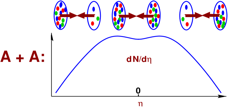
Figure 1: The CGC approach for nucleus - nucleus collision with the saturation of parton density.

The saturation scale is the main parameter of our approach and we need to understand clearly the energy dependence of $Q_{s}$ if we want to make predictions for the LHC energies. The first basic result on the behavior of this scale is the power-like energy dependence which follows directly from QCD for fixed QCD coupling. As was shown in a number of papers GLR ; BALE ; BSB ; BKL ; MUTR ; MP2003 ; DUR the energy dependence of the saturation scale does not depend on the details of the behavior of the parton system in the saturation domain but can be determined just by using the perturbative QCD approach in the BFKL region BFKL . Indeed, consider the dipole-target scattering amplitude in the double Mellin transform representation, namely,

$$N(y,r^{2})\,\,=\,\,\int\,\frac{d\omega\,d\gamma}{(2\pi i)^{2}}\,e^{\omega\,\ln(1/x)\,\,+\,\,(\gamma-1)\,\ln(r^{2}\Lambda^{2}_{QCD})}\,\,N(\omega,\gamma)\,\,.$$ (18)

The BFKL equation determines the value of $\omega$ at which $N(\omega,\gamma)$ has a pole:

$$\omega\,=\,\bar{\alpha}_{S}\,\chi(\gamma)$$ (19)

with a specific function $\chi$ which can be found e.g. in Ref. DUR ; we denote $\bar{\alpha}_{S}\equiv N_{c}\alpha_{S}/\pi$. To find the energy dependence of the saturation scale we first need to find a critical value of $\gamma=\gamma_{cr}$ defined by the equation GLR ; MUTR ; MP2003

$$\frac{\chi(\gamma_{cr})}{1-\gamma_{cr}}\,\,=\,\,-\,\frac{d\chi(\gamma_{cr})}{d\gamma}\,\,.$$ (20)

The meaning of this equation is the following: in the semi-classical approximation (see Ref. BKL and references therein) the scattering amplitude $N(y,\ln(r^{2}\Lambda^{2}_{QCD}))$ has the following form:

$$N(y,\xi\equiv\ln(r^{2}\Lambda^{2}_{QCD}))={\rm const}\times\ \exp\left[\omega(y,\xi)y-(1-\gamma(y,\xi))\xi\right].$$ (21)

The boundary of the saturation region is determined by the unique (critical) trajectory for the non-linear evolution equation in the $(y,\xi)$ plane for which the phase $v_{phase}=\omega(y,\xi)/(1-\gamma(y,\xi))$ and the group $v_{group}=-d\omega(y,\xi)/d\gamma(y,\xi)$ velocities are equal. The physical meaning of this trajectory can be illustrated by an analogy in geometrical optics: the boundary which it defines is similar to the focal reflecting surface (therefore, one can see that the surface of the Color Glass shines!). The equality of phase and group velocities thus gives the equation for the saturation scale:

$$\frac{d\ln(Q^{2}_{s}(x)/\Lambda^{2}_{QCD})}{d\,\ln(1/x)}\,\,=\,\,\bar{\alpha}_{S}\,\frac{\chi(\gamma_{cr})}{1-\gamma_{cr}}\,\equiv\,\lambda$$ (22)

For fixed $\alpha_{S}$ Eq. (22) leads to

$$Q^{2}_{s}(x)\,\,=Q^{2}_{0}\,\left(\frac{x_{0}}{x}\right)^{\lambda}$$ (23)

with $\lambda$ given by Eq. (22). The numerical analysis of the value of $\lambda$ can be found in Ref. DUR . The main conclusion from this analysis is the fact that the value of $\lambda$ is sensitive to higher order correction in $\alpha_{S}$. Therefore in this paper we choose to fix the value of $\lambda$ from the phenomenological approach, see Eq. (17); we consider Eq. (23) as a justification for the use of such a parameterization.

Another observation on the equation for the saturation scale Eq. (22) is that the value of $\gamma_{cr}$ is stable with respect to higher order corrections and almost does not depend on the value of the QCD coupling (see Ref. DUR ). This fact helps us to solve Eq. (22) in the case of running $\alpha_{S}$. The running of the coupling constant $\alpha_{S}$ leads to an additional dependence on $Q_{s}$ in the r.h.s. of Eq. (22); from Eq. (22) using the explicit form of the running coupling constant we find

$$\frac{d\ln(Q^{2}_{s}(W)/\Lambda^{2}_{QCD})}{d\,\ln(W/W_{0})}\,\,=\,\,{4\pi\over\beta_{2}}\,{\chi(\gamma_{cr})\over 1-\gamma_{cr}}\,{1\over\ln(Q^{2}_{s}(W)/\Lambda^{2}_{QCD})}\equiv{\delta\over\ln(Q^{2}_{s}(W)/\Lambda^{2}_{QCD})};$$ (24)

as a result, the dependence on $Q_{s}(W)$ has become explicit. Integrating Eq. (24) we obtain

$$Q^{2}_{s}(W)\,\,=\,\,\Lambda^{2}_{QCD}\,\,\,\exp\left(\sqrt{\,2\,\delta\,\ln(W/W_{0})\,\,+\,\,\ln^{2}(Q^{2}_{s}(W_{0})/\Lambda^{2}_{QCD})}\right),$$ (25)

where $Q^{2}_{s}(W_{0})$ is the saturation scale at the energy $W_{0}$ which we used as an initial condition in integrating Eq. (24). Here as well as in the rest of the paper $\Lambda^{2}_{QCD}$ is defined by $\alpha_{S}=4\pi/\beta_{2}\,\ln(Q^{2}/\Lambda^{2}_{QCD})$ and in numerical applications we took $\Lambda^{2}_{QCD}=0.04\ \ {\rm GeV}^{2}$ with $\beta_{2}=11-2/3\,N_{f}$ where $N_{f}=3$ is the number of fermions (number of colors $N_{c}=3$). We fix the value of $\delta$ through the empirical value of $\lambda$ as given by Eq. (23) and the value of saturation scale for the $Au$ nucleus at fixed energy of $W=130$ GeV, $y=0$, corresponding to the cut of $0-6\%$ of most central collisions, $Q_{s0}^{2}=2$ GeV², so that $\delta=\lambda\ln(Q^{2}_{s0}/\Lambda^{2}_{QCD})$.

The formula Eq. (25) reproduces all general features expected for the case of running QCD coupling; in particular, one can see that the saturation scale (25) does not depend on the mass number of the nucleus in the limit of high energies LERYD ; MUQA – the parton wave functions of different nuclei in this limit become universal. It is easy to generalize Eq. (25) to $y\neq 0$ by replacing $\ln(W/W_{0})$ by $\ln(W/W_{0})+y$; thus we have the following final formula for the case of running $\alpha_{S}$:

$$Q^{2}_{s}(y,W)=\Lambda^{2}_{QCD}\exp\left(\sqrt{2\lambda\ln(Q^{2}_{s0}/\Lambda^{2}_{QCD})[\ln(W/W_{0})+y]+\ln^{2}(Q^{2}_{s}(W_{0})/\Lambda^{2}_{QCD})}\right).$$ (26)

III.2 Formulae for the multiplicities

To derive the final expressions for the multiplicity it is convenient to re-write Eq. (14) using the fact that the main contribution to Eq. (14) is given by two regions of integration over $k_{t}$: $k_{t}\,\ll\,p_{t}$ and $|\vec{p}_{t}\,-\,\vec{k_{t}}|\,\ll\,p_{t}$; this leads to

$${dN\over dy} = {1\over S}\ \ \int dp_{t}^{2}\left(E{d\sigma\over d^{3}p}\right)\,=\,{1\over S}\ \ {4\pi N_{c}\alpha_{S}\over N_{c}^{2}-1}\ \times$$ (27)

$$\times \int{dp_{t}^{2}\over p_{t}^{2}}\ \left(\,\varphi_{A_{1}}(x_{1},p_{t}^{2})\,\,\int^{p_{t}}\,dk_{t}^{2}\ \varphi_{A_{2}}(x_{2},k_{t}^{2})\,\,+\,\,\varphi_{A_{2}}(x_{2},p_{t}^{2})\,\,\int^{p_{t}}\,dk_{t}^{2}\ \varphi_{A_{1}}(x_{1},k_{t}^{2})\,\right)\,\,=$$

$$= {1\over S}\ \ {4\pi N_{c}\alpha_{S}\over N_{c}^{2}-1}\ \,\int^{\infty}_{0}\,\,\frac{d\,p^{2}_{t}}{p^{4}_{t}}\,\,x_{2}G_{A_{2}}(x_{2},p^{2}_{t})\,\,x_{1}G_{A_{1}}(x_{1},p^{2}_{t})\,\,,$$

where we integrated by parts and used Eq. (13). In the KLMN treatment KN ; KL ; KLM ; KLN we assumed a simplified form of $xG$, namely,

$$xG(x;p^{2}_{t})\,\,=\,\,\left\{\begin{array}[]{l}\,\,\,\,{\displaystyle{\kappa\over\alpha_{S}(Q^{2}_{s})}}\,S\,p^{2}_{t}\,\,(1\,-\,x)^{4},\,\,\,\,\quad\quad p_{t}\,<\,Q_{s}(x)\,\,;\\ \\ \,\,\,\,{\displaystyle{\kappa\over\alpha_{S}(Q^{2}_{s})}}\,S\,Q^{2}_{s}(x)\,\,(1\,-\,x)^{4},\,\,\,\,\quad\quad p_{t}\,>\,Q_{s}(x)\,\,;\end{array}\right.$$ (31)

where the normalization coefficient $\kappa$ has been determined from the RHIC data on gold-gold collisions. We introduce the factor $(1\,-\,x)^{4}$ to describe the fact that the gluon density is small at $x\,\rightarrow\,1$ as described by the quark counting rules Brodsky ; Matveev .

We have checked that the simplified form of Eq. (31) is adequate for the calculations of multiplicity since it is dominated by the low momenta region. At high $p_{t}$ and small $x$, it was shown KLM that the quantum effects of the anomalous dimension could be extremely important. However, at moderate values of $x$ the simple form of Eq. (31) was used to calculate the $p_{t}$ spectra in proton-proton and electron-proton collisions in Ref. szc and the results appear very encouraging.

Having in mind Eq. (31), let us divide the $p_{t}$ integration in Eq. (14) in three different regions:

1. $p_{t}\,\,<\,\,Q_{s,min}$

   In this region both parton densities for $A_{1}$ and $A_{2}$ are in the saturation region. This region of integration gives

   $$\frac{dN}{dy}\,\,\propto\,\,\frac{1}{\alpha_{S}}\,S\,Q^{2}_{s,min}\,\,\propto\frac{1}{\alpha_{S}}\,\,N_{part}(A_{1})$$ (32)

   where we have used the fact that the number of participants is proportional to $SQ_{s}^{2}$, where $S$ is the area corresponding to a specific centrality cut.

2. $Q_{s,max}\,\,>\,\,p_{t}\,\,>\,\,Q_{s,min}$

   For these values of $p_{t}$ we have saturation regime for the nucleus $A_{2}$ for all positive rapidities while the nucleus $A_{1}$ is in the normal DGLAP evolution region. Neglecting anomalous dimension of the gluon density below $Q_{s,max}$, we have $\varphi_{A_{1}}(x_{1},k_{t}^{2})\,\,\propto\,\,\frac{1}{\alpha_{S}}\,\,S\,\,Q_{s,min}/k^{2}_{t}$ which for $y>y_{c}$ leads to

   $$\frac{dN}{dy}\,\,\propto\,\,\frac{1}{\alpha_{S}}\,S\,Q^{2}_{s,min}\,\ln\frac{Q^{2}_{s,max}}{Q^{2}_{s,min}}\,\,\propto\frac{1}{\alpha_{S}}\,\,N_{part}(A_{1})\,\,\ln\frac{Q^{2}_{s,max}}{Q^{2}_{s,min}}$$ (33)

   This region of integration will give the largest contribution.

3. $\,p_{t}\,\,>\,\,Q_{s,max}$

   In this region the parton densities in both nuclei are in the DGLAP evolution region.

Substituting Eq. (31) into Eq. (27) we obtain the following formula KL :

$$\frac{dN}{dy}\,\,=\,\,Const\,\times\,S\,\,Q^{2}_{s,min}(W,y)\,\,\frac{1}{\alpha_{S}(Q^{2}_{min}(W,y))}\,\times$$ (34)

$$\left[\left(1-\frac{Q_{s,min}(W,y)}{W}\,e^{y}\right)^{4}\,\,+\,\,\{\,\ln(Q^{2}_{max}(W,y)/Q^{2}_{s,min}(W,y))\,\,+\,\,1\,\}\,\left(1-\frac{Q_{s,max}(W,y)}{W}\,e^{y}\right)^{4}\,\right].$$

One can see two qualitative properties of Eq. (34). For $y\,>\,0$ and close to the fragmentation region of the nucleus $A_{1}$ , $Q_{s,min}=Q(A_{1})$ and the multiplicity is proportional to $N_{part}(A_{1})$, while in the fragmentation region of the nucleus $A_{2}$($y<0$) $Q_{s,min}=Q(A_{2})$ and $dN/dy\,\propto\,N_{part}(A_{2})$. We thus recover some of the features of the phenomenological ‘wounded nucleon’ model WNM .

IV Predictions

IV.1 Choice of the phenomenological parameters

As discussed above our main phenomenological parameter is the saturation momentum. An estimate of the value of the saturation momentum can be found from the following condition: the probability of interaction in the target (or ”the packing factor” of the partonic system) is equal to unity. The packing factor can be written in the following form:

$$P.F.\,\,=\,\,\frac{8\,\pi^{2}\,N_{c}\,\alpha_{S}(Q^{2})}{(N^{2}_{c}-1)\,Q^{2}}\,\,\frac{xG(x,Q^{2})}{\pi\,R^{2}}\,\,=\,\,\sigma\,\,\rho$$ (35)

where $\sigma$ is the cross section for dipole - target interaction (the size of the dipole is about 1/Q) and $\rho$ is the (two-dimensional) transverse density of partons inside the target of size $R$ (see e.g. Refs. KN ; KL for details).

In the case of the nucleon we do not know the value of $R$ or, in other words, we do not know the area which is occupied by the gluons ($S_{N}\,=\,\pi R^{2}$). However, we have enough information to claim that this area is less than the area of the nucleon ( $R$ is less than the electromagnetic radius of the proton). To substantiate this claim, let us recall for example the constituent quark model in which the gluons are distributed in the area determined by the small (relative to the size of the nucleon) size of the constituent quark. Having all these uncertainties in mind we use the phenomenological Golec-Biernat and Wuesthoff model GW to fix the value of the saturation moment in the case of the nucleon target. Namely, the value of the saturation moment for proton is equal $Q_{s}(P;y=0,W=200\,{\rm GeV})\,=\,0.37\,{\rm GeV}^{2}$. In Ref. KLND this value of the proton saturation momentum was used to describe the deuteron-gold collisions at RHIC energies.

In the case of the nuclear target the saturation momentum can be found from the expression for the packing factor

$$P.F.\,=\,\sigma\,\rho_{A}\,=\,\sigma\,\rho_{N}\,\frac{\rho_{part}}{2}\,\frac{S_{N}}{S_{A}}\,=\,Q^{2}_{S}(N)\,\frac{\rho_{part}}{2}\,\frac{S_{N}}{S_{A}}$$ (36)

As we have discussed we do not know the last factor ($S_{N}/S_{A}$) and therefore, Eq. (36) cannot help us to determine the value of the saturation momentum for a nucleus. We fixed the value of the saturation momentum from the description of the RHIC data on the multiplicity in gold-gold collisions, namely, $Q_{s}^{2}({\rm Gold},y=0,W=130\,GeV)\,=\,2.02\,{\rm GeV}^{2}$ for the centrality cut $0-6\%$ (see Refs. KN ; KL for details).

As far as energy dependence of the saturation scale is concerned, we used Eq. (16) and Eq. (26) with $\lambda$ given by the Golec-Biernat and Wuesthoff model ($\lambda=0.252$). However, we have to admit that the perturbative QCD estimates described above would lead to a larger value of $\lambda$ : $\lambda\,\approx\,\,0.37$. Such an uncertainty in the value of $\lambda$ leads to an error of about $12-15\%$ in our prediction for the proton-nucleus and nucleus-nucleus collisions at the LHC energies. For the proton-proton interaction it could generate an error as big as about $50\%$.

In our main formula given by Eq. (34) we have to fix the normalization factor. As discussed in Ref. KL theoretical estimates lead to a value of $Const$ in Eq. (34) which appears quite close to the value extracted by comparison with the RHIC data. In this paper we use the same normalization factor $Const$ as in KL , namely $Const\,S\,Q^{2}_{s,min}(W=200\,GeV,y=0)\,=\,0.615\,N_{part}$. We also need to note that the experimental measurement are done at fixed pseudo-rapidity $\eta$, not rapidity $y$; therefore, as discussed in Ref. KL we have to use the relation between $\eta$ and $y$, and to multiply Eq. (34) by the Jacobian of this transformation $h(\eta,Q_{s})$; see KL for details and explicit expressions.

Proton-proton collisions present an additional problem caused by the deficiency of the geometrical interpretation of $pp$ cross section. As mentioned above (see Eq. (14)) we calculated the ratio of the total inclusive cross section to the geometrical area of the interaction. This ratio is the measured multiplicity in the case of hadron-nucleus and nucleus-nucleus collisions. In the case of hadron-hadron interaction the multiplicity is the ratio of the inclusive cross section divided by the inelastic cross section. As discussed above, for $pp$ interactions we do not know the relation between the interaction area and the value of the inelastic cross section. To evaluate multiplicities in proton-proton interactions we do the following: (i) fix the ratio $S_{N}/\sigma_{in}$ at $W=200\,GeV$ using the data for $dN/dy(y=0)$; and (II) assume $S_{N}/\sigma_{in}\,\,\propto\,1/\sigma_{in}$ as far as the energy dependence is concerned. In other words we assume that the area $S_{N}$ does not depend on energy. The energy dependence of the inelastic cross section, including energies outside of the region accessible experimentally at present, was taken from Ref. GLMSF .

IV.2 Proton - proton collisions

IV.2.1 Rapidity distribution

Fig. 2 shows the calculated pseudorapidity distributions for the proton - proton (antiproton) collisions. The agreement with the experimental data is quite good despite the fact that $pp$ collisions present special difficulties for our approach since the value of the saturation momentum is rather small and non-perturbative corrections could be essential. We would like to point out however that the value of the saturation momentum for the proton reaches $\approx\,\,1\,GeV$ at the LHC energy. Our experience with RHIC data suggests that at such value of the saturation momentum our approach could apply with a reasonable accuracy. We thus expect that the very first $pp$ data from the LHC can provide an important test of the CGC ideas.

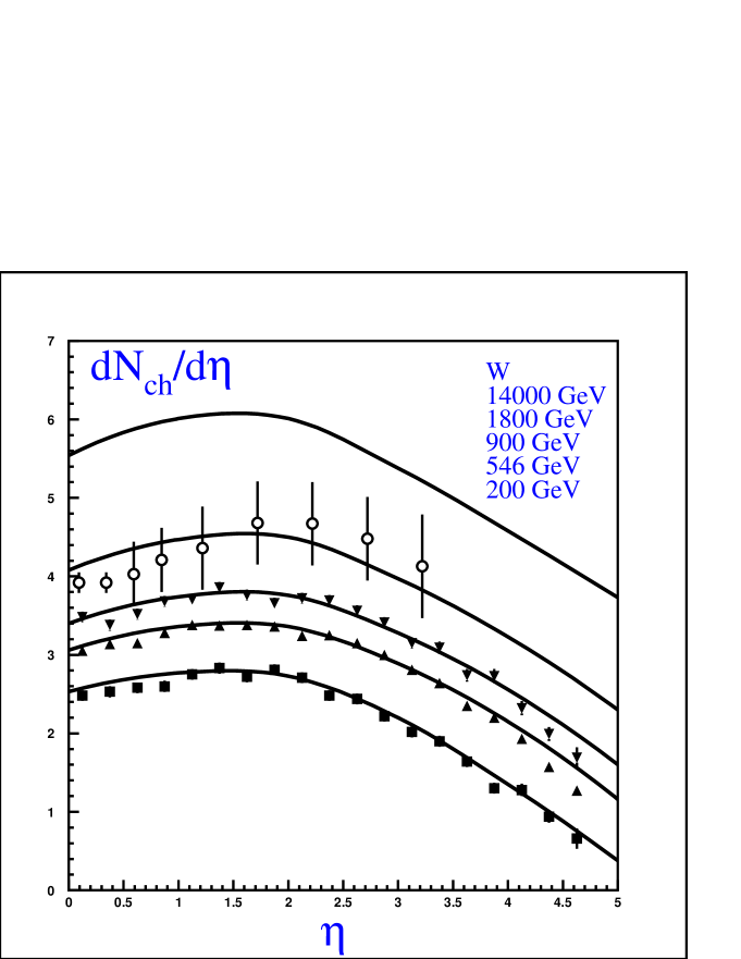
Figure 2: Rapidity dependence $dN/d\eta$ of charged hadron multiplicities in proton - proton (antiproton) collisions as a function of the pseudorapidity at different energies. The data are taken from Ref. RTABL .

In Fig. 3 we plot the value of $dN/d\eta$ at $\eta=0$ as a function of energy (in this plot we included also the available data at lower energies). The agreement with the experiment is seen to be quite good.

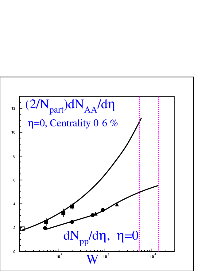
Figure 3: Energy dependence of charged hadron multiplicity $dN/d\eta$ at $\eta=0$ in proton - proton (antiproton) collisions and of charged hadron multiplicities per participant pair $(2/N_{part})\,dN/d\eta$ at $\eta=0$ for central nucleus-nucleus collisions. The vertical dotted lines mark the LHC energies for nucleus-nucleus collisions ($W=5500\,GeV$) and for proton-proton collisions ($W=14000\,GeV$). collisions. The experimental data are from Ref. RTABL ; REF1 .

IV.2.2 Total multiplicity

Integrating Eq. (34) over $\eta$ in the entire region of $\eta=-\ln W\,\div+\ln W$ we can calculate the total multiplicity in proton-proton ( antiproton) collisions. In Fig. 4 we present our calculation together with the experimental data taken from Refs. REF2 ; a good agreement with the data is seen in a wide range of energies. We would like to remind however that our predictions for the LHC energies could be as much as 1.5 times larger due to uncertainties in the energy behavior of the saturation scale discussed above.

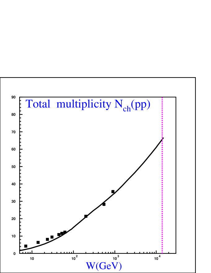
Figure 4: Energy dependence of total multiplicity in proton - proton (antiproton) collisions. The vertical dotted line marks the LHC energies for proton-proton collisions ($W=14000\,GeV$). collisions. The experimental data are taken from Ref. REF2 .

IV.3 Nucleus-nucleus collisions.

IV.3.1 Rapidity distribution $dN/dy$

Our prediction for lead-lead collision at the LHC energy is plotted in Fig. 5. The two sets of curves ( solid and dotted) describe the cases of fixed and running QCD coupling respectively. We consider the two predictions as the natural bounds for our predictions, and expect the data to be in between of these two curves. However, we would like to mention again that our predictions have systematic errors of about $12\div 15\%$ due to uncertainties in the energy dependence of the saturation scale.

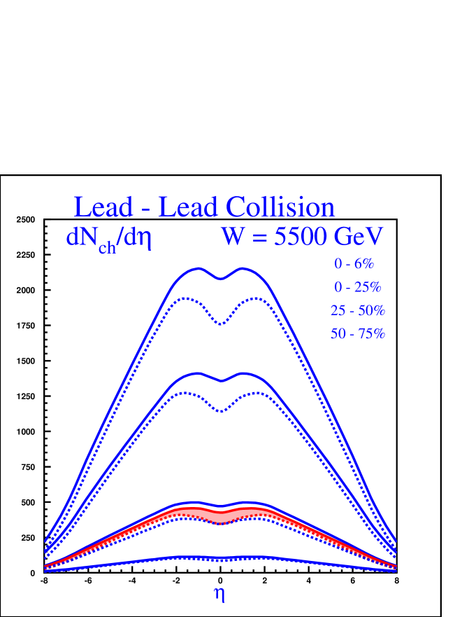
Figure 5: Rapidity dependence of $dN/d\eta$ lead-lead collisions at the LHC energy at different centrality cuts. The solid lines corresponds to the prediction using Eq. (16) for the energy dependence of the saturation scale while the dotted lines show the predictions for Eq. (26) for running QCD coupling. The shadowed area shows the prediction for the minimal bias event.

IV.3.2 Centrality dependence: $(2/N_{part})\,(dN_{ch}/d\eta)$

Fig. 6 shows our predictions for the $N_{part}$ dependence of the $(2/N_{part})\,(dN_{ch}/d\eta)$. This observable provides the most sensitive test of the value of the saturation scale and its dependence on the density of the participants.

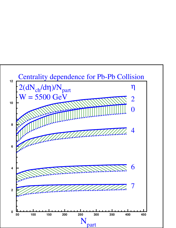
Figure 6: $N_{part}$ dependence of $(2/N_{ch})\,dN/d\eta$ for lead-lead collisions at the LHC energy at different rapidity cuts. The solid lines correspond to the prediction using Eq. (16) for the energy dependence of the saturation scale while the dotted lines show the predictions for Eq. (26) for running QCD coupling. The shadowed areas show the spread of our predictions.

Fig. 3 shows the energy dependence of $(2/N_{ch})\,(dN/d\eta)$ at $\eta=0$. One can see that we are able to describe the current experimental data. Note that if we neglect the difference between rapidity and pseudorapidity, $(2/N_{ch})\,(dN/d\eta)$ at $\eta=0$ is given by a very simple formula KLN :

$$\frac{2}{N_{part}}\,\frac{dN_{ch}}{dy}\,|_{y=0}\,\, = \,\,0.87\,\left(\frac{W}{W_{0}}\right)^{\lambda}\,\ln(Q_{s}^{2}(A,W,y=0)/\Lambda_{QCD}^{2})=$$ (37)

$$= 0.87\,\left(\frac{W}{130}\right)^{0.252}\,\left(3.93\,\,+\,\,0.252\,\,\ln(W/130)\,\right)$$

This formula is in good agreement with the existing experimental data.

IV.4 Proton - nucleus collisions

Fig. 7 shows our prediction for the proton-nucleus collisions at W=5500 GeV. In section 2 we described the procedure of computing the number and density of participants in this case; to evaluate the relevant value of the saturation momentum, we take account of the energy dependence to extrapolate from RHIC to the LHC energy. For example, the density of participants $\rho_{part}\approx 1.84\ {\rm fm}^{-2}$ corresponds to the saturation scale of $Q_{s}^{2}\approx 2\,{\rm GeV}^{2}(5500/200)^{0.252}$  $\approx 4.6\,{\rm GeV}^{2}$.

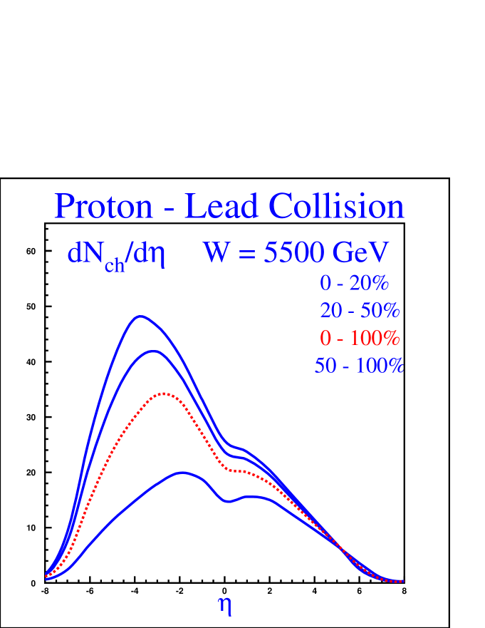
Figure 7: Rapidity dependence of $dN/d\eta$ proton-lead collisions at the LHC energy at different centrality cuts. The dotted line corresponds to the minimal bias event.

V Conclusions

In this paper we have provided a complete set of predictions for the multiplicity distributions at the LHC basing on the CGC approach. In our approach, parton saturation results in a relatively weak, compared to most other approaches, dependence of the multiplicity on energy. As one can see from Fig. 8 we expect rather small number of produced hadrons in comparison with the alternative approaches. What is the uncertainty in our predictions? We would like to recall the estimates for the uncertainty in our calculations at the LHC energies given above: $12\div 15\%$ for nucleus-nucleus and hadron-nucleus collisions, and a large value of $40\div 50\%$ for the proton-proton collisions. These uncertainties arise from the poor theoretical knowledge of the energy dependence of the saturation scale, and in the case of $pp$ collisions also from the uncertainties in the application of the geometrical picture.

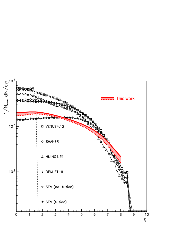
Figure 8: Comparison of our predictions for charged hadron multiplicities in central ($b\leq 3$ fm) $Pb-Pb$ collisions with the results from other approaches, as given in Ref.REVAP

We hope that our estimates will be useful for the interpretation of the first results from LHC experiments. As illustrated in Fig. 8, a measurement of multiplicity at the LHC will provide a very important test of the CGC approach.

VI Acknowledgements

The work of D.K. was supported by the U.S. Department of Energy under Contract No. DE-AC02-98CH10886. E.L. and M.N. are grateful to the RIKEN-BNL Research Center and the Nuclear Theory Group at BNL for hospitality and support during the period when this work was done. The work opf E.L. was supported in part by the grant of Israeli Science Foundation ,founded by Israeli Academy of Science and Humanity.

References

- (1) L. V. Gribov, E. M. Levin and M. G. Ryskin, Phys. Rep. 100 (1983) 1.
-
(2)
A.H. Mueller and J. Qiu, Nucl.Phys. B 268 (1986) 427;
J.-P. Blaizot and A.H. Mueller, Nucl. Phys. B 289 (1987) 847. - (3) L. McLerran and R. Venugopalan, Phys. Rev. D 49 (1994) 2233; 3352; D 50 (1994) 2225.
-
(4)
Ia. Balitsky, Nucl.Phys. B463 (1996) 99;
Yu. Kovchegov, Phys. Rev. D60 (2000) 034008. -
(5)
J. Jalilian-Marian, A. Kovner, A. Leonidov and H. Weigert,
Phys. Rev. D59 (1999) 014014
[arXiv:hep-ph/9706377]; Nucl. Phys. B504 (1997) 415
[arXiv:hep-ph/9701284];
E. Iancu, A. Leonidov and L. D. McLerran, Phys. Lett. B510 (2001) 133 [arXiv:hep-ph/0102009]; Nucl. Phys. A692 (2001) 583 [arXiv:hep-ph/0011241];
H. Weigert, Nucl. Phys. A703 (2002) 823 [arXiv:hep-ph/0004044]. - (6) I. G. Bearden [BRAHMS Collaboration], Phys. Rev. Lett. 87 (2001) 112305; arXiv:nucl-ex/0403050; Phys. Rev. Lett. 88, 202301 (2002) [arXiv:nucl-ex/0112001]; Phys. Lett. B 523, 227 (2001) [arXiv:nucl-ex/0108016]; R. Debbe [BRAHMS Collaboration], arXiv:nucl-ex/0405018; I. Arsene et al. [BRAHMS Collaboration], arXiv:nucl-ex/0403005.
- (7) A. Bazilevsky [PHENIX Collaboration], arXiv:nucl-ex/0304015; Nucl. Phys. A 715, 486 (2003);
- (8) A. Milov [the PHENIX Collaboration], Nucl. Phys. A 698, 171 (2002) [arXiv:nucl-ex/0107006]; K. Adcox et al. [PHENIX Collaboration], Phys. Rev. Lett. 87, 052301 (2001); Phys. Rev. Lett. 86, 3500 (2001).
- (9) B. B. Back et al. [PHOBOS Collaboration], Phys. Rev. Lett. 85, 3100 (2000); Phys. Rev. C 65, 061901 (2002); Phys. Rev. Lett. 87, 102303 (2001); Phys. Rev. Lett. 85, 3100 (2000); arXiv:nucl-ex/0406017; arXiv:nucl-ex/0405027; R. Nouicer et al. [PHOBOS Collaboration], arXiv:nucl-ex/0403033; M. D. Baker [PHOBOS Collaboration], arXiv:nucl-ex/0212009.
- (10) Z. b. Xu [STAR Collaboration], arXiv:nucl-ex/0207019; C. Adler et al. [STAR Collaboration], Phys. Rev. Lett. 87, 112303 (2001); L. S. Barnby [STAR Collaboration], arXiv:nucl-ex/0404027.
- (11) D. Kharzeev and M. Nardi, Phys. Lett. B 507 (2001) 121.
- (12) D. Kharzeev and E. Levin, Phys. Lett. B 523 (2001) 79.
- (13) D. Kharzeev, E. Levin and M. Nardi, “The onset of classical QCD dynamics in relativistic heavy ion collisions,” hep-ph/0111315.
- (14) D. Kharzeev, E. Levin and L. McLerran, Phys. Lett. B 561 (2003) 93.
- (15) D. Kharzeev, Y. V. Kovchegov and K. Tuchin, Phys. Rev. D 68, 094013 (2003); arXiv:hep-ph/0405045.
- (16) K. J. Eskola, H. Niemi, P. V. Ruuskanen and S. S. Rasanen, Nucl. Phys. A 715 (2003) 561 [arXiv:nucl-th/0210005].
- (17) T. Hirano and Y. Nara, “Hydrodynamic afterburner for the color glass condensate and the parton energy loss,” arXiv:nucl-th/0404039.
- (18) Yu.V. Kovchegov, Phys. Rev. D 54 (1996) 5463; J. Jalilian-Marian, A. Kovner, L. McLerran, H. Weigert, Phys.Rev. D55 (1997) 5414; E. Iancu and L. McLerran, Phys.Lett. B510 (2001) 145; A. Krasnitz and R. Venugopalan, Phys. Rev. Lett.84 (2000) 4309; E. Levin and K. Tuchin, Nucl. Phys. B573 (2000) 833; A693 (2001) 787; A691 (2001) 779; A.H. Mueller,“Parton saturation: An overview,” hep-ph/0111244; E. Iancu, A. Leonidov and L. D. McLerran, Nucl. Phys. A692 (2001) 583, hep-ph/0011241; E. Iancu, K. Itakura and L. McLerran, Nucl. Phys. A708 (2002) 327, hep-ph/0203137.
- (19) E. Levin and M. Lublinsky, Nucl. Phys. A730 (2004) 191 [arXiv:hep-ph/0308279].
- (20) E. Iancu and A. H. Mueller, Nucl. Phys. A730 (2004) 460, 494, [arXiv:hep-ph/0308315],[arXiv:hep-ph/0309276].
- (21) M. Kozlov and E. Levin, Nucl. Phys. A 739 (2004) 291 [arXiv:hep-ph/0401118].
- (22) A. H. Mueller and A. I. Shoshi, “Small-x physics beyond the Kovchegov equation,” arXiv:hep-ph/0402193;“Small-x physics near the saturation regime,”. talk at 39th Rencontres de Moriond on QCD and High-Energy Hadronic Interactions, La Thuile, Italy, 28 Mar - 4 Apr 2004 arXiv:hep-ph/0405205.
- (23) E. Laenen and E. Levin, Ann. Rev. Nuc. Part. Sci. 44 (1994) 199; Yu. V. Kovchegov and D. Rischke, Phys. Rev. C56 (1997) 1084; M. Gyulassy and L. McLerran, Phys. Rev. C56 (1997) 2219; Yu. V. Kovchegov and A. H. Mueller, Nucl. Phys. B529 (1998) 451 M. A. Braun, Eur. Phys. J. C16 (2000) 337, hep-ph/0010041, hep-ph/0101070; Yu. V. Kovchegov, Phys. Rev. D64 (2000) 114016; Yu. V. Kovchegov and K. Tuchin, Phys. Rev. D65 (2002) 074026 hep-ph/0111362.
- (24) D. N. Triantafyllopoulos, Nucl. Phys. B 648 (2003) 293 [arXiv:hep-ph/0209121].
- (25) V. A. Khoze, A. D. Martin, M. G. Ryskin and W. J. Stirling, “The spread of the gluon k(t)-distribution and the determination of the saturation scale at hadron colliders in resummed NLL BFKL,” arXiv:hep-ph/0406135.
- (26) A. Bialas, M. Bleszynski and W. Czyz, Nucl.Phys. B111 (1976) 461.
- (27) D. Kharzeev, C. Lourenco, M. Nardi and H. Satz, Z. Phys. C 74 (1997) 307, [arXiv:hep-ph/9612217].
- (28) E. Gotsman, E. Levin and U. Maor, Phys. Lett. B 452 (1999) 387 [arXiv:hep-ph/9901416].
- (29) K. Golec-Biernat and M. Wüsthof, Phys. Rev. D59 (1999) 014017; Phys. Rev. D60 (1999) 114023; A. Stasto, K. Golec-Biernat and J. Kwiecinski, Phys. Rev. Lett. 86 (2001) 596.
- (30) J. Bartels and E. Levin, Nucl. Phys. B387 (1992) 617.
- (31) J. Bartels, G. A. Schuler and J. Blumlein, Z. Phys. C50 (1991) 91; Nucl. Phys. Proc. Suppl. 18C (1991) 147.
- (32) S. Bondarenko, M. Kozlov and E. Levin, Nucl. Phys. A727 (2003) 139 [arXiv:hep-ph/0305150].
- (33) A. H. Mueller and D. N. Triantafyllopoulos, Nucl. Phys. B640 (2002) 331 [arXiv:hep-ph/0205167];
- (34) S. Munier and R. Peschanski, Phys. Rev. Lett. 91, 232001 (2003) [arXiv:hep-ph/0309177].
-
(35)
E. A. Kuraev, L. N. Lipatov, and F. S. Fadin,it Sov. Phys. JETP
45 (1977) 199 ;
Ya. Ya. Balitsky and L. N. Lipatov, Sov. J. Nucl. Phys. 28 (1978) 22 . - (36) E. M. Levin and M. G. Ryskin, Yad. Fiz. 45 (1987) 234 [Sov. J. Nucl. Phys. 45 (1987) 150].
- (37) A. H. Mueller, Nucl. Phys. A 724 (2003) 223 [arXiv:hep-ph/0301109].
- (38) S. J. Brodsky and G. R. Farrar, Phys. Rev. Lett. 31, 1153 (1973).
- (39) V. A. Matveev, R. M. Muradian and A. N. Tavkhelidze, Lett. Nuovo Cim. 7, 719 (1973).
- (40) A. Szczurek, “From unintegrated gluon distributions to particle production in hadronic collisions at high energies,” arXiv:hep-ph/0309146; Acta Phys. Polon. B34 (2003) 3191 arXiv:hep-ph/0304129, B35 (2004) 161 arXiv:hep-ph/0311175.
- (41) D. Kharzeev, E. Levin and M. Nardi, Nucl. Phys. A 730 (2004) 448 [arXiv:hep-ph/0212316].
- (42) S. Eidelman et al. [Particle Data Group Collaboration], “Review of particle physics,” Phys. Lett. B 592 (2004) 1.
-
(43)
B.B.Back et al (Phobos Collab.), Phys. Rev. Lett. 85 (2000)
3100 ;
Quark Matter 2004, Oakland, Jan. 11-17,2004 - (44) B.B.Back et al (Phobos Collab.), nucl-ex/0301017.
- (45) N. Armesto and C. Pajares, Int. J. Mod. Phys. A 15 (2000) 2019 [arXiv:hep-ph/0002163].