Hadronic interactions of the $J/\psi$ and Adler’s theorem

Abstract

Effective Lagrangian models of charmonium have recently been used to estimate dissociation cross sections with light hadrons. Detailed study of the symmetry properties reveals possible shortcomings relative to chiral symmetry. We therefore propose a new Lagrangian and point out distinguishing features amongst the different approaches. Moreover, we test the models against Adler’s theorem, which requires, in the appropriate limit, the decoupling of pions from the theory for the normal parity sector. Using the newly proposed Lagrangian, which exhibits $SU_{L}(N_{f})\times\,SU_{R}(N_{f})$ symmetry and complies with Adler’s theorem, we find dissociation cross sections with pions that are reduced in an energy dependent way, with respect to cases where the theorem is not fulfilled.

I Introduction

The theoretical study of matter under extreme conditions enjoys a wide range of application, from the physics of the early Universe, to that of relativistic nuclear collisions. The latter offer the tantalizing possibility of recreating in the laboratory the conditions that prevailed roughly a microsecond after the Big Bang. The theory of the strong interaction, Quantum Chromodynamics (QCD), predicts a phase transition from normal hadronic matter to a plasma of quarks and gluons kl03 . To find a signature of this new state of matter represents a task which has generated tremendous activity both in theory and in experiment. Of the many signals put forward as probes of the quark-gluon plasma, the suppression of the $J/\psi$ yield enjoys a popular status mat86 .

Indeed, since charmonium is predominantly produced in the early stage of the nuclear collisions through hard processes, it acts as a probe for the subsequent stages. The original idea was that the presence of a quark-gluon plasma (QGP) will screen the long-range confining force between $c$-$\bar{c}$, leading to the decoherence of the pair mat86 . This suppression mechanism was later augmented by the possibility of charmonium dissociation by hard gluons in a deconfined medium ks94 . In the interpretation of the early centrality-dependent $J/\psi$ absorption observed by the NA38 collaboration na38 , those suppression mechanisms were not manifest and nuclear absorption sufficed to understand the data. But, this scenario says nothing about the effects of the late hadronic phase. Indeed, also accounting for final state interactions can go a long way in reproducing the NA50 suppression pattern na50 observed subsequently in Pb + Pb collisions, provided the $J/\psi$ cross-sections with hadronic matter are of the order of one to a few millibarns arm98 ; cap02 . In those experiments, it is fair to say that the presence of a quark-gluon plasma is still ambiguous. Thus, in order to identify the true nature of a possibly new phase, it appears necessary to quantify the $J/\psi$-light hadron interaction. This requirement on the $J/\psi$ cross-sections with light mesons is not a trivial one to satisfy, as there are no direct experimental measurements. One has to rely on theoretical calculations based, for example, on QCD sum-rules dur03 , on quark-potential models mar95 ; won01 , or on effective mesonic Lagrangians mat95 ; kh00 ; hag00 ; lin00 ; oh01 . These lead typically to cross-sections from a few tenths of a millibarn to a few millibarns near threshold dur03 .

Specifically, for the effective mesonic Lagrangians found in hag00 ; lin00 ; oh01 , once form factors have been folded-in to account for short-range interactions, the dissociation cross-section by pions reaches a few millibarns. But concerns have been raised about using such models: (i) the $SU(4)$ symmetry used to describe the pseudoscalar and vector meson interactions is questionable as it is broken, (ii) the form factors accounting for the finite size of the mesons do not proceed from the formalism as in other models dur03 ; won01 , and (iii) the $J/\psi+\pi\rightarrow D^{*}+\bar{D}$ process does not vanish in the soft-pion limit for non-degenerate vector meson masses as expected from Adler’s theorem nav01 . All of those can be addressed, but it is the purpose of this article to expand on the last point and show that, even in the degenerate vector mass limit, the pions’ decoupling in the soft limit does not necessarily follow for amplitudes constructed from the normal parity content of the Lagrangians found in hag00 ; lin00 ; oh01 . Consequently, we propose an alternative charmonium Lagrangian implementing the extended $SU_{L}(4)\times SU_{R}(4)$ chiral symmetry for which the theorem holds for a degenerate vector mass spectrum.
Our paper is organized as follows: we first present two models implementing the $SU_{L}(N_{f})\times SU_{R}(N_{f})$ chiral symmetry and one implementing only the $SU_{V}(N_{f})$ symmetry. Having introduced the pseudoscalar mesons as Goldstone bosons in all these models, we note that for $SU_{L}(N_{f})\times SU_{R}(N_{f})$ invariant normal parity Lagrangians, the pseudoscalars must decouple from the theory in the zero-momentum limit. We explicitly show that at the amplitude level for the process $\rho^{0}+\pi^{+}\rightarrow\rho^{0}+\pi^{+}$, the $SU_{L}(2)\times SU_{R}(2)$ chirally symmetric models obey the soft-pion theorem, while the isospin-only invariant model does not. We then digress on electromagnetic current conservation, and show that it can be implemented in all the models. Bearing in mind that we wish to study the implementation of pions’ decoupling in effective charmonium Lagrangians, we review the most commonly used effective Lagrangians in hadronic $J/\psi$ suppression, and show that they are not invariant under the $SU_{L}(4)\times SU_{R}(4)$ symmetry, but rather only under $SU_{V}(4)$. We explore the consequences of implementing the extended chiral symmetry by comparing the cross-section for the $J/\psi+\pi$ absorption process obtained in our two formulations. Finally, in Appendix A, we show that the amplitude for the $J/\psi+\pi$ absorption process does vanish in the degenerate vector meson mass limit for the extended chiral symmetric case, but not the $SU_{V}(4)$. We re-derive the result of Ref. nav01 for the case of a non-degenerate vector mass spectrum. We then explicitly check in Appendix B that the Ward identity holds for both $SU_{V}(4)$ and $SU_{L}(4)\times SU_{R}(4)$ models. In Appendix C, a discussion about fixing coupling constants is presented.

II EFFECTIVE MESONIC LAGRANGIANS

II.1 $SU_{L}(N_{f})\boldmath{\mbox{$\times$}}SU_{R}(N_{f})$ Lagrangian with pseudoscalar, vector and axial vector mesons

To build a $SU_{L}(N_{f})\times SU_{R}(N_{f})$ symmetric Lagrangian with pseudoscalar, vector and axial vector mesons mei88 , we start with the non-linear $\sigma$ model

$$\mathcal{L}=\frac{1}{8}F_{\pi}^{\,2}{\rm{\rm Tr}}\left(\partial_{\mu}U\partial^{\mu}U^{\dagger}\right),$$ (1)

where $U=\exp(2i\phi/F_{\pi})$ and $\phi=\frac{T^{a}\phi^{a}}{\sqrt{2}}$, $T^{a}$ are the $SU(N_{f})$ generators, and we introduce the vector and axial vector mesons by minimal coupling of the right- and left-handed vector fields

$$A_{L\mu}=\frac{1}{2}\left(V_{\mu}+A_{\mu}\right)$$ (2)

$$A_{R\mu}=\frac{1}{2}\left(V_{\mu}-A_{\mu}\right).$$ (3)

The resulting Lagrangian

$$\mathcal{L}=\frac{1}{8}F_{\pi}^{\/2}{\rm Tr}\left[D_{\mu}UD^{\mu}U^{\dagger}\right]-\frac{1}{2}{\rm{\rm Tr}}\left[F_{\mu\nu L}F^{\mu\nu}_{L}+F_{\mu\nu R}F^{\mu\nu}_{R}\right],$$ (4)

where $D_{\mu}U=\partial_{\mu}U-igA^{L}_{\mu}U+igUA^{R}_{\mu}$, $F^{R,L}_{\mu\nu}$ are the non-Abelian field strength tensors, and $g$ is the universal gauge coupling, is then invariant under a $SU_{L}(N_{f})\times SU_{R}(N_{f})$ transformationkay85

$$U \rightarrow U_{L}UU^{\dagger}_{R}$$ (5)

$$A_{\mu}^{L} \rightarrow U_{L}A^{L}_{\mu}U^{\dagger}_{L}+\frac{i}{g}U_{L}\partial_{\mu}U^{\dagger}_{L}$$ (6)

$$A_{\mu}^{R} \rightarrow U_{R}A^{R}_{\mu}U^{\dagger}_{R}+\frac{i}{g}U_{R}\partial_{\mu}U^{\dagger}_{R}.$$ (7)

We note here that $SU_{V}(N_{f})$ and $SU_{A}(N_{f})$ are subgroups of the full $SU_{L}(N_{f})\times SU_{R}(N_{f})$ group. To account for the right- and left-handed mesons’ masses, we add the symmetry-invariant term

$$m_{0}^{\/2}{\rm Tr}\left[A_{\mu L}A^{\mu}_{L}+A_{\mu R}A^{\mu}_{R}\right].$$ (8)

We could also supplement the Lagrangian with the pseudoscalar mass term mei88

$$\frac{1}{8}F_{\pi}^{\,2}{\rm Tr}\left(M(U+U^{\dagger}-2)\right),$$ (9)

where $M$ is the pseudoscalar mass matrix. But this term explicitly breaks the symmetry, and thus will be considered as a correction (as lifting the mass degeneracy of the vector mesons). Expanding the Lagrangian and removing the mixing between the pseudoscalar and axial vector fields via

$$A_{\mu}\rightarrow A_{\mu}+\frac{g\tilde{F}_{\pi}}{2m_{0}^{2}}\partial_{\mu}\phi,\mbox{ }\phi\rightarrow Z^{-1}\tilde{\phi},\mbox{ }F_{\pi}\rightarrow Z^{-1}\tilde{F}_{\pi},\mbox{ }Z^{2}=\left(1-\frac{g^{2}\tilde{F}_{\pi}^{\,2}}{4m_{0}^{2}}\right)$$ (10)

yields

$$\mathcal{L} = \frac{1}{2}{\rm Tr}\left[\partial_{\mu}\phi\partial^{\mu}\phi\right]-\frac{1}{4}{\rm Tr}\left[F^{V}_{\mu\nu}F^{\mu\nu}_{V}+F^{A}_{\mu\nu}F^{\mu\nu}_{A}\right]$$ (11)

$$+ \frac{1}{2}m_{V}^{2}{\rm Tr}\left[V_{\mu}^{2}\right]+\frac{1}{2}m_{A}^{2}{\rm Tr}\left[A_{\mu}^{2}\right]$$

$$+ \mathcal{L}_{V\phi\phi}+\mathcal{L}_{AV\phi}+\mathcal{L}_{VV\phi\phi}+\cdots\,,$$

where the tildes were dropped for simplicity and the degenerate masses are defined as $m_{V}^{2}=m_{0}^{2}$, and $m_{A}^{2}=m_{V}^{2}/Z^{2}$. To the above Lagrangian other non-minimal terms can be added and are necessary to fit $\pi$, $\rho$, and $a_{1}$ phenomenology gom84 . But the Lagrangian of Eq. (11) will be sufficient for our purposes.

II.2 $SU_{L}(N_{f})\boldmath{\mbox{$\times$}}SU_{R}(N_{f})$ Lagrangian with pseudoscalar and vector mesons

In the previous section the axial mesons were introduced as the chiral partners of the $\rho$ fields resulting in a linear realization of the symmetry gai69 . In the present case, since the desired $SU_{L}(N_{f})\times SU_{R}(N_{f})$ Lagrangian will involve only pseudoscalar and vector mesons, both will then have to transform non-linearly under the symmetry. This is similar to building an effective low-energy theory with the $\pi$ field transforming non-linearly under the axial group, or equivalently by imposing a constraint gai69 ; wei68 . The second approach will be favoured here by gauging-away the axial mesons kay85 . But before doing so, we add to Eq. (4) the locally-invariant term

$$\gamma{\rm Tr}\left(F_{\mu\nu}^{L}UF^{\mu\nu R}U^{\dagger}\right)$$ (12)

and the mass term of Eq. (8) with the further addition

$$B{\rm Tr}\left[A_{L\mu}UA^{\mu}_{R}U^{\dagger}\right].$$ (13)

The second mass term is non-minimal and is introduced to account for $\rho$-meson phenomenology in the final Lagrangian kay85 . To remove the axial mesons we set $U_{L}=U^{1/2}=\zeta$ and $U_{R}=U^{-1/2}=\zeta^{\dagger}$ in Eqs. (5-7) giving

$$U = \zeta 1\zeta$$ (14)

$$A_{\mu}^{L} = \zeta\rho_{\mu}\zeta^{\dagger}+\frac{i}{g}\zeta\partial_{\mu}\zeta^{\dagger}$$ (15)

$$A_{\mu}^{R} = \zeta^{\dagger}\rho_{\mu}\zeta+\frac{i}{g}\zeta^{\dagger}\partial_{\mu}\zeta\,.$$ (16)

This amounts to imposing the $SU_{L}(N_{f})\times SU_{R}(N_{f})$ invariant constraint

$$\mathcal{D}_{\mu}U^{\dagger}=0.$$ (17)

The new vector field $\rho_{\mu}$ then transforms in the usual way under the vector symmetry, namely

$$\rho_{\mu}\rightarrow K\rho_{\mu}K^{\dagger}+\frac{i}{g}K\partial_{\mu}K^{\dagger},$$ (18)

where $K\in SU_{V}(N_{f})$, but transforms non-linearly under the axial-vector subgroup. Substituting the new field definitions and normalizing the vector and pseudoscalar kinetic terms by choosing

$$\gamma = \frac{3}{4},\mbox{ }\frac{2m_{0}^{2}-B}{g^{2}F_{\pi}^{\,2}}=\frac{1}{2}$$ (19)

yields

$$\mathcal{L} = -\frac{1}{4}{\rm Tr}\left[F_{\mu\nu}(\rho)F^{\mu\nu}(\rho)\right]+\frac{1}{2}m_{V}^{2}{\rm Tr}[\rho_{\mu}^{2}]$$ (20)

$$+ \frac{F_{\pi}^{\,2}}{4}(1+k){\rm Tr}\left[\partial_{\mu}\zeta\partial^{\mu}\zeta\right]+i\frac{F_{\pi}^{\,2}\,g_{V\phi\phi}}{2}{\rm Tr}\left[\rho^{\mu}\left(\partial_{\mu}\zeta\zeta^{\dagger}+\partial_{\mu}\zeta^{\dagger}\zeta\right)\right]$$

$$+ \frac{F_{\pi}^{\,2}}{4}(1-k){\rm Tr}\left[\zeta^{\dagger}\partial^{\mu}\zeta^{\dagger}\zeta\partial_{\mu}\zeta\right],$$

where the parameters are defined as $m_{V}^{2}=2B+4m_{0}^{2}$, $g_{V\phi\phi}=m_{V}^{2}/gF_{\pi}^{\,2}$ and $g=g_{V\phi\phi}/k$, and the field strength tensor is $F_{\mu\nu}(\rho)=\partial_{\mu}\rho_{\nu}-\partial_{\nu}\rho_{\mu}-ig[\rho_{\mu},\rho_{\nu}]$ sch86 . Notice the extra parameter $k$, owing to the introduction of the non-minimal vector meson mass term. As with the Lagrangian of Eq. (11), this Lagrangian of pseudoscalars and vector mesons is globally invariant under $SU_{L}(N_{f})\times SU_{R}(N_{f})$, and consequently under the $SU_{V}(N_{f})$ subgroup.

II.3 $SU_{V}(N_{f})\boldmath{\mbox{$\,$}}$ Lagrangian with pseudoscalar and vector mesons

The two preceding Lagrangians encode $SU_{L}(N_{f})\times SU_{R}(N_{f})$ symmetry. For the purpose of reviewing the effective Lagrangian models used to calculate charmonium dissociation, we now build a $SU_{V}(N_{f})$ invariant-only Lagrangian by gauging the non-linear $\sigma$ model with the vector meson field sak69

$$\mathcal{L}=\frac{F_{\pi}^{\,2}}{8}{\rm Tr}\left[D_{\mu}UD^{\mu}U^{\dagger}\right]-\frac{1}{4}{\rm Tr}[F_{V}^{\mu\nu}F^{V}_{\mu\nu}] + \frac{1}{2}m_{V}^{2}{\rm Tr}[V_{\mu}^{2}],$$ (21)

where $D_{\mu}U=\partial_{\mu}U-i\frac{g}{2}[V_{\mu},U]$ and $F^{V}_{\mu\nu}=\partial_{\mu}V_{\nu}-\partial_{\nu}V_{\mu}-i\frac{g}{2}[V_{\mu},V_{\nu}]$. This Lagrangian is invariant under a global $SU_{V}(N_{f})$ transformation, but not under the full $SU_{L}(N_{f})\times SU_{R}(N_{f})$ symmetry group ($SU_{V}(N_{f})$ is a subgroup of this group). It also exhibit a $PPVV$ contact interaction, while Eq. (20) has no such term.

III Adler’s Theorem

A spontaneously broken symmetry not only implies the existence of Goldstone bosons, but also constrains their low-energy behaviour. Here we will consider the transition amplitude for emitting one Goldstone boson (the proof can easily be extended to more than one). Following Weinberg wei95 , we first note that the current operator can create a Goldstone boson

$$\left<0|J^{\mu}(x)|B\right>=i\frac{Fq^{\mu}}{(2\pi)^{3}2E}e^{-iq\cdot x}$$ (22)

where F is the decay constant. We expect the matrix element $\left<\beta|J^{\mu}(x)|\alpha\right>$ to then have a pole term. Indeed, in general, we can write

$$\left<\alpha|J^{\mu}(0)|\beta\right>=N^{\mu}_{\beta\alpha}+i\frac{Fq^{\mu}}{q^{2}}M^{B}_{\beta\alpha},$$ (23)

where $M^{B}_{\beta\alpha}$ is the desired transition amplitude for emitting one Goldstone boson, and $N^{\mu}_{\beta\alpha}$ is assumed to be the pole-free contribution. Applying the current conservation constraint, we then find that

$$M^{B}_{\beta\alpha}=\frac{i}{F}q_{\mu}N^{\mu}_{\beta\alpha}$$ (24)

and we see that as $q\rightarrow 0$ the RHS vanishes. Historically, this property was first studied by Adler adl65 , and rests on the assumption that $N^{\mu}_{\beta\alpha}$ has no singularity as $q\rightarrow 0$. This is not valid in general, since a pole may arise through the insertion of the current operator on an external line sak69 . $M^{B}_{\beta\alpha}$ can then have a non-vanishing contribution in the soft limit due to emission of a soft Goldstone boson off an external line. But this is not the case for $SU_{L}(N_{f})\times SU_{R}(N_{f})$ normal parity mesonic Lagrangians where there are no vertices such as $\phi^{3}$ or $VV\phi$ (see Eq. 20).
Thus, for the normal parity Lagrangians where the underlying symmetry is $SU_{L}(N_{f})\times SU_{R}(N_{f})$, we expect that transition amplitudes will vanish in the pseudoscalar zero-momentum limit bur00 , up to corrections from coupling to other non-symmetric invariant gauge fields, such as the electromagnetic field, and in general any non-invariant terms (e.g. pseudoscalar masses). In the following subsections, we will explicitly check that decoupling occurs for the process $\pi^{+}+\rho^{0}\rightarrow\pi^{+}+\rho^{0}$ in the two chiral-invariant Lagrangians of Eqs. (11-20), but not for the isospin-invariant model of Eq. (21).

III.1 Chiral model with $\pi$, $\rho$, and $a_{1}$ mesons

Figure 1: $\rho^{0}+\pi^{+}\rightarrow\rho^{0}+\pi^{+}$.

The process we want to consider, namely $\pi^{+}(p_{1})+\rho^{0}(q_{1})\rightarrow\pi^{+}(p_{2})+\rho^{0}(q_{2})$, involves 5 tree-level diagrams for the given particle content: $\pi$- and $a_{1}$-mediated exchanges both in $s$ and $t$ channels, and through a 4-point interaction (Fig 1). We start with the relevant interaction terms from the Lagrangian of Eq. (11)

$$\mathcal{L}_{V\phi\phi} = -\frac{ig}{2}{\rm Tr}\Big{[}V^{\mu}[\phi,\partial_{\mu}\phi]\Big{]}+\frac{igZ^{2}}{2m_{V}^{2}}{\rm Tr}\Big{[}(\partial_{\mu}V_{\nu}-\partial_{\nu}V_{\mu})\partial^{\mu}\phi\partial^{\nu}\phi\Big{]}$$ (25)

$$\mathcal{L}_{AV\phi} = \frac{ig^{2}\,F_{\pi}}{4m_{V}^{2}}{\rm Tr}\Big{[}(\partial_{\mu}V_{\nu}-\partial_{\nu}V_{\mu})[A^{\mu},\partial^{\nu}\phi]+(\partial_{\mu}A_{\nu}-\partial_{\nu}A_{\mu})[V^{\mu},\partial^{\nu}\phi]\Big{]}\Big{]}$$ (26)

$$- \frac{ig^{2}F_{\pi}}{4Z^{2}}{\rm Tr}\Big{[}V^{\mu}[A_{\mu},\phi]\Big{]}$$

$$\mathcal{L}_{VV\phi\phi} = \frac{g^{2}}{8}\frac{g^{2}F_{\pi}^{\,2}}{4m_{0}^{4}}{\rm Tr}\Big{[}[V^{\mu},V^{\nu}][\partial_{\mu}\phi,\partial_{\nu}\phi]+[V^{\mu},\partial^{\nu}\phi][\partial_{\mu}\phi,V_{\nu}]+[V^{\mu},\partial^{\nu}\phi][V_{\mu},\partial_{\nu}\phi]\Big{]}$$ (27)

$$- \frac{g^{2}}{8Z^{2}}{\rm Tr}\Big{[}[V_{\mu},\phi]^{2}\Big{]}.$$

From here we extract the off-shell vertex functions

$$\Gamma^{1}_{\mu} = -\frac{g}{\sqrt{2}}\left[k_{\mu}+p_{\mu}-\frac{(1-Z^{2})}{m_{V}^{2}}\left(q\cdot kp_{\mu}-q\cdot pk_{\mu}\right)\right]$$ (28)

$$\Gamma^{2}_{\mu\nu} = -\frac{ig}{\sqrt{2}}\frac{(1-Z^{2})^{\frac{1}{2}}}{m_{V}}\left\{(m_{A}^{2}+q^{2}-k^{2})g_{\mu\nu}-q_{\mu}q_{\nu}+k_{\mu}k_{\nu}\right\}$$ (29)

$$\Gamma^{3}_{\mu\nu} = 2\left[\frac{g^{2}}{2}\frac{(1-Z^{2})}{2m_{V}^{2}}\left\{-2p_{1}\cdot p_{2}g_{\mu\nu}+p_{1\mu}p_{2\nu}+p_{2\mu}p_{1\nu}\right\}+\frac{g^{2}}{2Z^{2}}g_{\mu\nu}\right]$$ (30)

for $\pi^{+}(p)+\rho^{0}(q)\rightarrow\pi^{+}(k)$, $\pi^{+}(p)+\rho^{0}(q)\rightarrow a_{1}^{+}(k)$, and the four-point interaction, respectively. The resulting five off-shell amplitudes are then

$$i\mathcal{M}^{1}_{\mu\nu} = i\Gamma^{1\dagger}_{\mu}\frac{i}{s-m_{\pi}^{2}}i\Gamma^{1}_{\nu}$$ (31)

$$i\mathcal{M}^{2}_{\mu\nu} = i\Gamma^{1\dagger}_{\mu}\frac{i}{t-m_{\pi}^{2}}i\Gamma^{1}_{\nu}$$ (32)

$$i\mathcal{M}^{3}_{\mu\nu} = i\Gamma^{2\dagger}_{\mu\alpha}\frac{-i[g^{\alpha\beta}-(p_{1}+q_{1})^{\alpha}(p_{1}+q_{1})^{\beta}/m_{A}^{2}]}{s-m_{A}^{2}}i\Gamma^{2}_{\nu\beta}$$ (33)

$$i\mathcal{M}^{4}_{\mu\nu} = i\Gamma^{2\dagger}_{\mu\alpha}\frac{-i[g^{\alpha\beta}-(q_{2}-p_{1})^{\alpha}(q_{2}-p_{1})^{\beta}/m_{A}^{2}]}{t-m_{A}^{2}}i\Gamma^{2}_{\nu\beta}$$ (34)

$$i\mathcal{M}^{5}_{\mu\nu} = i\Gamma^{3}_{\mu\nu}.$$ (35)

Having now the full amplitude for the given process, we wish to see if the pseudoscalar decoupling theorem holds. The presence of the contact term in the 4-point interaction leads us to expect cancellations to occur as we let one of the pions’ 4-momentum go to zero. Stated differently, since the $\rho$-meson was introduced in a chirally symmetric way by adding its chiral partner (i.e. $a_{1}$), the transition amplitude relies on help from the $a_{1}$ in what amounts to a delicate cancellation allowing the pion to decouple. To show this, we contract the amplitudes with the appropriate polarization vectors, and then let $p_{2}\rightarrow 0$ (a similar proof can be shown to hold for $p_{1}\rightarrow 0$). First it is seen that the amplitudes involving the $\pi$-exchange go to zero because of transversality (i.e $\epsilon(q)\cdot q$). For $a_{1}$-exchange in the $s$-channel we find (the same result is true for the $t$-channel)

$$i\mathcal{M}_{3} = \epsilon^{*\mu}(q_{2})\left[i\Gamma^{2\dagger}_{\mu\alpha}(p_{2}\rightarrow 0)\frac{-i\left[g^{\alpha\beta}-\frac{q_{2}^{\alpha}q_{2}^{\beta}}{m_{A}^{2}}\right]}{m_{V}^{2}-m_{A}^{2}}i\Gamma^{2}_{\nu\beta}\right]\epsilon^{\nu}(q_{1})$$ (36)

$$= -\frac{ig^{2}}{2}\frac{1}{m_{V}^{2}}\epsilon^{*\mu}(q_{2})\left[m_{A}^{2}g_{\mu\nu}-q_{1\mu}q_{1\nu}+\frac{q_{1}\cdot q_{2}}{m_{A}^{2}}q_{2\mu}q_{1\nu}+\frac{m_{V}^{2}}{m_{A}^{2}}q_{2\mu}q_{2\nu}\right]\epsilon^{\nu}(q_{1})$$

$$= -\frac{ig^{2}}{2Z^{2}}\epsilon^{*}(q_{2})\cdot\epsilon(q_{1}).$$

The last line comes about again due to the orthogonality condition. Finally, the 4-point interaction reads

$$i\mathcal{M}_{5}=\frac{ig^{2}}{Z^{2}}\epsilon^{*}(q_{2})\cdot\epsilon(q_{1}),$$ (37)

and thus the full amplitude is shown to vanish as expected. Note the cancellation between the 4-point interaction and the $a_{1}$ channels. In summary, even though the pions are not coupled through gradient coupling for all interaction terms, the net amplitude still vanishes due to intricate cancellations amongst all the channels.

III.2 Chiral model with $\pi$ and $\rho$ mesons

In this model there are only two diagrams, namely $s\,$- and $t\,$-channels of pion exchange. The relevant interaction Lagrangian is

$$\mathcal{L}_{\rho\pi\pi}=-i\frac{g_{\rho\pi\pi}}{2}{\rm Tr}\left[\rho^{\mu}[\phi,\partial_{\mu}\phi]\right]\,$$ (38)

and the extracted vertex for the s- and t- channels is

$$\Gamma_{\mu}^{{}^{\prime}1}=-\frac{g_{\rho\pi\pi}}{\sqrt{2}}\left(p_{\mu}+k_{\mu}\right),$$ (39)

with $k=p+q$ and $k=p-q$, respectively. The two amplitudes are then

$$i\mathcal{M}^{1}_{\mu\nu}=i\Gamma^{{}^{\prime}1\dagger}_{\mu}\frac{i}{s-m_{\pi}^{2}}i\Gamma^{{}^{\prime}1}_{\nu}$$ (41)

$$i\mathcal{M}^{2}_{\mu\nu}=i\Gamma^{{}^{\prime}1\dagger}_{\mu}\frac{i}{t-m_{\pi}^{2}}i\Gamma^{{}^{\prime}1}_{\nu}\,.$$ (42)

We immediately see that the soft pion theorem holds separately for each amplitude when the proper polarization vectors are contracted with the amplitudes.

III.3 Isospin-invariant model with $\pi$ and $\rho$

Here the interaction Lagrangians are given by

$$\mathcal{L}_{\rho\pi\pi} = -i\frac{g}{2}{\rm Tr}\Big{[}V^{\mu}[\phi,\partial_{\mu}\phi]\Big{]}$$ (43)

$$\mathcal{L}_{\rho\rho\pi\pi} = -\frac{g^{2}}{8}{\rm Tr}\Big{[}[V_{\mu},\phi]^{2}\Big{]}.$$ (44)

We note that the three-point interaction is identical in structure to the ones from the previous sections, and the derived amplitude from these terms disappears in the appropriate limit. The difference lies here in the additional 4-point interaction. Indeed, in the zero-momentum limit for the pion its contribution is non-vanishing, and therefore the pions do not decouple. It is then expected that the behaviour of the cross-section for the process near threshold to be different from the one calculated in the chiral models.

IV ELECTROMAGNETIC CURRENT CONSERVATION

We now wish to add electromagnetism to all three models and to investigate the validity of vector meson dominance (VMD) sak69 .

IV.1 $SU_{L}(N_{f})\boldmath{\mbox{$\times$}}SU_{R}(N_{f})$ Lagrangian with pseudoscalar, vector and axial vector mesons

The fields transform under $U_{EM}(1)$ as sch86 :

$$\delta a_{\mu} = \frac{1}{e}\partial_{\mu}\epsilon$$ (45)

$$\delta U = i\epsilon[Q,U]$$ (46)

$$\delta A_{\mu}^{L,R} = i\epsilon[Q,A_{\mu}^{L,R}]+\frac{1}{g}Q\partial_{\mu}\epsilon,$$ (47)

where $a_{\mu}$ is the electromagnetic field and $Q$ is the appropriate quark charge matrix. Using Witten’s iterative method wit83 , Eq. (11) can be made invariant provided we add the following terms sch86

$$\Delta_{L}=-\frac{2em_{0}^{2}}{g}a^{\mu}{\rm Tr}\left[Q(A_{\mu}^{L}+A_{\mu}^{R})\right]+\frac{2em_{0}^{2}}{g^{2}}a_{\mu}^{2}{\rm Tr}Q^{2}\,.$$ (48)

By explicitly expanding the first term one obtains kro67

$$\mathcal{L}_{\rm VMD}=-\sqrt{2}\frac{e}{g}m_{V}^{2}a^{\mu}\rho^{0}_{\mu}+\cdots\,.$$ (49)

The above interaction term is precisely Sakurai’s original formulation of vector meson dominance.

IV.2 $SU_{L}(N_{f})\boldmath{\mbox{$\times$}}SU_{R}(N_{f})$ Lagrangian with pseudoscalar and vector mesons

We now turn to the non-linear model. Here we must add extra-terms due to the non-minimal mass term introduced in the mesonic Lagrangian of Eq. (20). The counter terms added to make the Lagrangian invariant are

$$\Delta_{NL} = -\frac{2em_{0}^{2}}{g}a^{\mu}{\rm Tr}\left[Q(A_{\mu}^{L}+A_{\mu}^{R})\right]-\frac{B}{g}a^{\mu}{\rm Tr}\left[Q\left(UA_{\mu}^{R}U^{\dagger}+U^{\dagger}A_{\mu}^{L}U\right)\right]$$ (50)

$$+ \frac{2em_{0}^{2}}{g^{2}}a_{\mu}^{2}{\rm Tr}Q^{2}+\frac{Be^{2}}{g^{2}}a_{\mu}^{2}{\rm Tr}\left[QUQU^{\dagger}\right].$$

Then using the expressions for $A_{\mu}^{L}$, $A_{\mu}^{R}$ and $U$ in terms of $\rho$ and $\phi$, we find

$$\Delta_{NL} = -ea^{\mu}\left[kgF_{\pi}^{\,2}{\rm Tr}[Q\rho_{\mu}]+i(1-k/2){\rm Tr}\left[Q[\phi,\partial_{\mu}\phi]\right]-\frac{g_{\rho\pi\pi}}{2}{\rm Tr}\left[Q\left[\phi,[\phi,\rho_{\mu}]\right]\right]\right]+\cdots\,.$$ (51)

We first note that beyond the vector-photon coupling (first term), there can be a direct $\phi\phi\gamma$ contribution (second term). Moreover a 4-point interaction exists (third term) of type $V\phi\phi\gamma$ and is essential for current conservation in processes such as $\rho^{0}+\pi^{+}\rightarrow\pi^{+}+\gamma$.

IV.3 $SU_{V}(N_{f})\boldmath{\mbox{$\,$}}$ Lagrangian with pseudoscalar and vector mesons

Finally, we examine the $SU_{V}(N_{f})$-invariant Lagrangian of Eq. (21). Under the electromagnetic gauge transformations, since the photon couples only to the vector field, the counter terms are also given by $\Delta_{L}$ (Eq. 48).

V CHARMONIUM EFFECTIVE LAGRANGIANS

We now review the effective Lagrangians used to calculate the $J/\psi$ dissociation rate in a hadronic gas hag00 ; lin00 ; oh01 . The underlying hypothesis of all these models is to assume that the pseudoscalar and vector meson fields are in multiplets of $SU(4)$. The interactions are then built from these by using the same techniques outlined in previous sections. Coupling constants for the various interactions are fixed either empirically or using symmetry arguments hag00 ; lin00 ; oh01 . Moreover, to model short range interactions, form factors are introduced (e.g. hag00 ). Overall, the models differ in their methods for fixing the coupling constants, their choice of form factors and implementation, and in their abnormal parity interaction content.
The three approaches can be summarized as Lagrangians where (i) both axial vector and vector mesons are present, but the interaction vertices with axial vector mesons are dropped oh01 , (ii) non-minimal mass terms are added and the axial mesons are gauged-away by imposing a $SU_{L}(4)\times SU_{R}(4)$ symmetric constraint in a similar fashion as in Section II. C hag00 , and (iii) only the vector mesons are introduced through gauge-coupling as in section II. B lin00 . Comparing the Lagrangians in references hag00 ; lin00 ; oh01 , we see that, up to a constant redefinition, they all lead to the same normal parity $SU_{V}(4)$ invariant-only Lagrangian, namely that of Eq. (21) not01 . Indeed, all these approaches lead to the pseudoscalars not decoupling for the $P+V\rightarrow P+V$ process in the zero-momentum pseudoscalar limit for degenerate vector mesons masses. In the first approach, the theorem is not respected because the axial vector mesons are omitted, and as it was shown that virtual axial vector meson exchange plays an essential role in canceling the non-vanishing zero-momentum contribution of the $PPVV$ vertex. In the second approach, the theorem was again not respected because the third non-minimal mass term of Eq. (2.6) in hag00 is not globally invariant under $SU_{L}(4)\times SU_{R}(4)$ symmetry, which leads to a non-vanishing zero-momentum $PPVV$ contribution. And in the third case, the Lagrangian is globally invariant only under $SU_{V}(4)$, but not the extended symmetry lin002 . Thus, none of the amplitudes extracted from these Lagrangians obeys the decoupling theorem in the degenerate vector mass limit, neither for the $J/\psi+\pi\rightarrow D^{*}(\bar{D}^{*})+\bar{D}(D)$ nor the $\rho+\pi\rightarrow\rho+\pi$ processes.

VI Comparative ANALYSIS

We have shown that the effective Lagrangian models found in the literature hag00 ; lin00 ; oh01 are all $SU_{V}(4)$ invariant (in the degenerate mass limit), but not $SU_{L}(4)\times SU_{R}(4)$ invariant. Here we will compare the $J/\psi+\pi$ cross-section as calculated within the models of Eq. (20) and Eq. (21). In the former, we need to consider three diagrams (Fig. 2), while for the latter, the contact interaction is absent (as expected from previous discussions). In Appendix A, we further address the pseudoscalars’ decoupling in the soft momentum limit, and in Appendix B we investigate the electromagnetic current conservation for the related $\gamma+\pi\rightarrow\bar{D}+D^{*}$ process.

Figure 2: $J/\psi+\pi\rightarrow D^{*}(\bar{D}^{*})+\bar{D}(D)$.

VI.1 $SU_{V}(4)$ model

Defining the pseudoscalar and vector field matrices as in hag00 , the relevant interaction terms from Eq. (21) are

$$\mathcal{L}_{J/\psi DD} = ig_{J/\psi DD}\psi^{\mu}(D\partial_{\mu}\bar{D}-\partial_{\mu}D\bar{D})$$ (52)

$$\mathcal{L}_{\pi DD^{*}} = ig_{\pi DD^{*}}D^{*\mu}(\partial_{\mu}\pi\bar{D}-\pi\partial_{\mu}\bar{D})+h.c.$$ (53)

$$\mathcal{L}_{J/\psi D^{*}D^{*}} = ig_{J/\psi D^{*}D^{*}}[\psi^{\mu}(\partial_{\mu}D^{*}_{\nu}\bar{D}^{*\nu}-D^{*\nu}\partial_{\mu}\bar{D}^{*}_{\nu})+\psi^{\mu}(D^{*\nu}\partial_{\nu}\bar{D}^{*}_{\mu}-\partial_{\mu}D^{*}_{\nu}\bar{D}^{*\nu})$$ (54)

$$- \partial_{\mu}\psi_{\nu}(D^{*\mu}\bar{D}^{*\nu}-D^{*\nu}\bar{D}^{*\mu})]$$

$$\mathcal{L}_{J/\psi D^{*}D\pi} = -g_{J/\psi D^{*}D\pi}\psi^{\mu}(D^{*}_{\mu}\pi\bar{D}+D\pi\bar{D}^{*}_{\mu}),$$ (55)

where $\psi$ is the $J/\psi$ field, the isospin doublets are oh01 $\bar{D}^{T}=(\bar{D}^{0},D^{-})$, $D=(D^{0},D^{+})$, and similarly for the vector particles, and $\pi=\frac{1}{\sqrt{2}}\vec{\tau}\cdot\vec{\pi}$. Provided the symmetry is exact, we have also

$$g_{J/\psi DD}=g_{J/\psi D^{*}D^{*}}=\frac{g}{\sqrt{3}},\mbox{ }g_{\pi DD^{*}}=\frac{g}{2},\mbox{ }g_{J/\psi D^{*}D\pi}=\frac{g^{2}}{2\sqrt{3}}\,.$$ (56)

The amplitudes for the absorption process are then

$$i\mathcal{M}^{1}_{\mu\nu} = +ig_{J/\psi DD}g_{\pi DD^{*}}\frac{(2p_{2\nu}-q_{1\nu})(2p_{1\mu}-q_{2\mu})}{(q_{1}-p_{2})^{2}-m_{D}^{2}}$$ (57)

$$i\mathcal{M}^{2}_{\mu\nu} = -ig_{J/\psi D^{*}D^{*}}g_{\pi DD^{*}}\frac{[(2q_{2}-q_{1})_{\nu}g_{\mu\lambda}+(2q_{1}-q_{2})_{\mu}g_{\lambda\nu}-(q_{1}+q_{2})_{\lambda}g_{\mu\nu}](p_{1\lambda}(1+\Delta)+p_{2\lambda}(1-\Delta))}{(q_{1}-q_{2})^{2}-m_{D}^{*2}}$$ (58)

$$i\mathcal{M}^{3}_{\mu\nu} = -ig_{J/\psi D^{*}D\pi}g_{\mu\nu},$$ (59)

where $\Delta=(m_{D}^{2}-m_{\pi}^{2})/m_{D^{*}}^{2}$. In Appendix A we show that for degenerate vector meson masses, the full amplitude does not vanish in the soft-momentum limit. Rather, there is a left-over contact term due to the third diagram.

VI.2 $SU_{L}(4)\boldmath{\mbox{$\times$}}SU_{R}(4)$ model

For the $SU_{L}(4)\times SU_{R}(4)$ invariant Lagrangian of Eq. (20), the interaction terms are given by Eq (52)-(54), but now with

$$g_{J/\psi DD}=\frac{g_{V\phi\phi}}{\sqrt{3}}=\frac{kg}{\sqrt{3}},\mbox{ }g_{J/\psi D^{*}D^{*}}=\frac{2g}{\sqrt{3}},\mbox{ }g_{\pi DD^{*}}=\frac{g_{V\phi\phi}}{2}=\frac{kg}{2}.$$ (60)

With these, the two relevant amplitudes are those of Eqs. (57) and (58). Note that we can map the $SU_{V}(4)$ couplings to those above by letting $k=2$ and setting $g\rightarrow g/2$.

VI.3 Results

The first step is to fix the coupling constants of the two models. This is done in Appendix C. Also, to account for short range interactions form factors would have to be folded in hag00 ; lin00 ; oh01 . But, since we are here interested in the effect of the implementation of the symmetry group, they will not be introduced. The differential isospin-averaged cross-section is then given by

$$\frac{d\sigma}{dt}=\frac{1}{128\pi sp^{2}_{1}}\mathcal{M}^{\mu\nu}\mathcal{M}^{\alpha\beta}\left[g_{\mu\alpha}-\frac{q_{2\mu}q_{2\alpha}}{m^{2}_{D^{*}}}\right]\left[g_{\nu\beta}-\frac{q_{1\nu}q_{1\beta}}{m^{2}_{J/\psi}}\right],$$ (61)

where the appropriate model-dependent squared amplitude is used, an isospin factor of two has been included and the centre of mass momentum is

$$p^{2}_{1}=\frac{1}{4s}\lambda(s,m^{2}_{\pi},m^{2}_{J/\psi})$$ (62)

and the triangle function is $\lambda(x,y,z)=x^{2}-2x(y+z)+(y-z)^{2}$. Integrating over the kinematical range defined by

$$t_{\pm}=m_{\pi}^{2}+m_{D^{*}}^{2}-\frac{1}{2s}(s+m_{\pi}^{2}-m_{J/\psi}^{2})(s+m_{D^{*}}^{2}-m_{D}^{2})\pm\frac{1}{2s}\lambda^{1/2}(s,m_{\pi}^{2},m_{J/\psi}^{2})\lambda^{1/2}(s,m_{D}^{2},m_{D^{*}}^{2})$$ (63)

gives the total cross-section. Carrying this to completion for the two models yields Fig. 3. We see an energy-dependent reduction in the cross sections across the relevant domain and to quote a specific number we note that at $\sqrt{s}=5$ GeV the cross-section is reduced by about 40% going from the $SU_{V}(4)$ model to the $SU_{L}(4)\times SU_{R}(4)$ model.

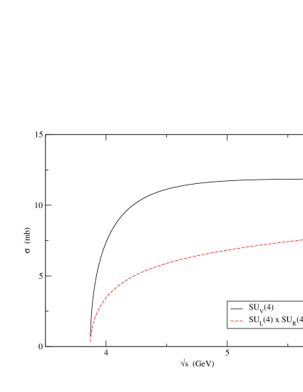
Figure 3: Isospin-averaged cross-section for $J/\psi+\pi\rightarrow(D^{*}+\bar{D})+(\bar{D}^{*}+D)$.

VII CONCLUSION AND OUTLOOK

Modeling low-energy hadron physics is particularly challenging when there is limited experimental input available for constraints. This is the current situation in the charm sector as the only measurement relevant for fixing coupling constants in the model is the decay width for $D^{*}\rightarrow\/D\pi$ cleo . We have therefore invoked symmetries and general theorems. In particular, we have checked for full $SU_{L}(4)\times\/SU_{R}(4)$ symmetry and the appropriate limit to test for compliance with Adler’s theorem. We found that none of the published models can do this, and we therefore proposed a new effective Lagrangian—the first one which does encode complete four-flavour chiral symmetry and Adler’s theorem. Our interest here has been solely to quantify the effect of these. A complete calculation including form factors and a longer list of reactions is a topic for a separate study.

Since Adler’s theorem is relevant at low-energy, the near-threshold cross sections are expected to be affected the most. We found the cross section for $J/\psi+\pi\rightarrow(D^{*}+\bar{D})+h.c.\,$ to be reduced as compared to a choice of Lagrangian which does not encode the full flavour chiral symmetry and does not obey Adler’s theorem. The reduction is energy dependent, but seems to be a few tens of percents from threshold to $\sqrt{s}$ = 5 GeV. In a full calculation the size of this reduction might not persist when one takes into account not only form factors, but also abnormal parity interactions and symmetry breaking effects (e.g. pseudoscalar masses and non-degenerate vector mass spectrum).

Abnormal parity interactions may play an important role near threshold. Indeed, it was shown that Adler’s theorem breaks down if a soft Goldstone boson can be inserted on an external line. This is expected to happen for abnormal parity Lagrangians where a $VV\phi$ vertex exists. The abnormal parity contribution to the $J/\psi+\pi$ amplitude will then not vanish in the soft limit. The problem in including these interactions lies again in the lack of experimental data to fix the coupling strengths.

Symmetry breaking effects are also expected to be important since the underlying $SU_{L}(4)\times SU_{R}(4)$ is broken. Work is currently being done to include the physical mass of the vector meson within this formalism, while insisting that Adler’s theorem hold for pions in normal parity interactions.

It will also be important in the future to take this formalism to completion by implementing covariant hadronic form factors computed within the same effective Lagrangian or perhaps other approaches. Ultimately, the outlook for this line of study is to estimate the dissociation cross sections with all the light hadrons, with finite size effects incorporated, and then to input the results into a dynamical model for heavy ion reactions to finally address the question of $J/\psi$ survivability in the hadronic phase (primarily mesonic matter). For then, one would have a more complete understanding of the $J/\psi$ yield and therefore know what it implies about QGP formation.

Appendix A Decoupling of the pion in the $J/\psi+\pi\rightarrow D^{*}+\bar{D}$ process

Here we look at the soft-momentum limit of the full amplitude for the absorption process $J/\psi+\pi$ under the degenerate-vector meson mass condition. Again, we set one of the pseudoscalars’ 4-momentum to zero (i.e. here $p_{1}$, but the proof is identical for $p_{2}$). As shown in a Section III B, for on-shell vector particles, the first amplitude goes to zero. For the second amplitude we have

$$i\mathcal{M}^{2}_{\mu\nu}(p_{1}\rightarrow 0)=-ig_{J/\psi D^{*}D^{*}}g_{\pi DD^{*}}\frac{[(2q_{2}-q_{1})_{\nu}g_{\mu\lambda}+(2q_{1}-q_{2})_{\mu}g_{\lambda\nu}-(q_{1}+q_{2})_{\lambda}g_{\mu\nu}]p_{2\lambda}(1+\Delta)}{(q_{1}-q_{2})^{2}-m_{D}^{*2}}.\\$$ (64)

Using momentum conservation in the first and second terms and noting that $t=(q_{1}-q_{2})^{2}=(p_{2}-p_{1})^{2}$ yields

$$i\mathcal{M}^{2}_{\mu\nu}(p_{1}\rightarrow 0)=-ig_{J/\psi D^{*}D^{*}}g_{\pi DD^{*}}\frac{[(q_{2}-p_{2})_{\nu}g_{\mu\lambda}+(q_{1}+p_{2})_{\mu}g_{\lambda\nu}-(q_{1}+q_{2})_{\lambda}g_{\mu\nu}]p_{2\lambda}(1+\Delta)}{p_{1}^{2}-2p_{1}\cdot p_{2}+p_{2}^{2}-m_{D}^{*2}},\\$$ (65)

which reduces to

$$i\mathcal{M}^{2}_{\mu\nu}(p_{1}\rightarrow 0) = \frac{ig_{J/\psi D^{*}D^{*}}g_{\pi DD^{*}}}{m_{D^{*2}}-m_{D}^{2}}[q_{2\nu}p_{2\mu}-p_{2\nu}p_{2\mu}+q_{1\mu}p_{2\nu}+p_{2\mu}p_{2\nu}-(q_{1}+q_{2})\cdot p_{2}g_{\mu\nu}](1+\Delta)$$ (66)

$$= \frac{ig_{J/\psi D^{*}D^{*}}g_{\pi DD^{*}}}{m_{D^{*2}}-m_{D}^{2}}[q_{2\nu}p_{2\mu}+q_{1\mu}p_{2\nu}-(q_{1}^{2}-q_{2}^{2})g_{\mu\nu}](1+\Delta)\,.$$

Contracting with the polarization vectors gives

$$i\mathcal{M}^{2}(p_{1}\rightarrow 0) = \frac{ig_{J/\psi D^{*}D^{*}}g_{\pi DD^{*}}}{m_{D^{*2}}-m_{D}^{2}}(1+\Delta)\epsilon^{*\nu}(q_{2})[q_{2\nu}p_{2\mu}+q_{1\mu}p_{2\nu}-(q_{1}^{2}-q_{2}^{2})g_{\mu\nu}]\epsilon^{\mu}(q1)$$ (67)

$$= \frac{ig_{J/\psi D^{*}D^{*}}g_{\pi DD^{*}}}{m_{D^{*2}}-m_{D}^{2}}(1+\Delta)\epsilon^{*}(q_{2})\cdot\epsilon(q_{1})[m_{D^{*}}^{2}-m_{J/\psi}^{2}]$$

$$= 0.$$

In the $SU_{L}(4)\times SU_{R}(4)$ model, the pseudoscalar meson thus decouples. But for the $SU_{V}(4)$, where $\mathcal{M}^{3}$ (contact term) is present, the full amplitude does not disappear. Note also that, as pointed out in nav01 , unless the underlying vector meson masses are degenerate (i.e. the vector mesons are arranged in $SU(4)$ multiplets) we have a residual contact term due to the second amplitude, and consequently the amplitude will not vanish when one of the pseudoscalar momenta goes to zero.

Appendix B Electromagnetic current conservation for the $\gamma+\pi^{+}\rightarrow\bar{D}^{0}+D^{*+}$ process

The proof that the electromagnetic current is conserved for this process in the $SU_{V}(4)$ model is given in hag00 . The authors invoke VMD, which we have shown to be exact in this model. For the $SU_{L}(4)\times SU_{R}(4)$ model, we have five amplitudes to consider (Fig. 4): two which involve three intermediate particles (i.e. $\rho^{0}$, $\omega$, and $J/\psi$), two $s\,$-channel contributions (one dominated by the $\rho$-meson and one through a direct $\gamma\pi\pi$ vertex), and a 4-point interaction.

Figure 4: Diagrams to be considered in the $SU_{L}(4)\times SU_{R}(4)$ model for the process $\gamma+\pi^{+}\rightarrow D^{*+}+\bar{D}^{0}$.

More specifically, the five amplitudes are

$$\mathcal{M}_{\mu\nu}^{1} = -\frac{iekgF_{\pi}^{\,2}\,g^{2}_{V\phi\phi}}{2}\left[\frac{1}{4}+\frac{1}{12}-\frac{1}{3}\right]\frac{[g_{\nu\alpha}-q_{1\nu}q_{1\alpha}/m_{V}^{2}]}{q_{1}^{2}-m_{V}^{2}}\frac{(2p_{2\alpha}-q_{1\alpha})(2p_{1\mu}-q_{2\mu})}{(q_{1}-p_{2})^{2}-m_{D}^{2}}=0$$

$$\mathcal{M}_{\mu\nu}^{2} = -\frac{iekgF_{\pi}^{\,2}g\,g_{V\phi\phi}}{2}\left[\frac{1}{2}-\frac{1}{6}+\frac{2}{3}\right]\frac{[g_{\nu\alpha}-q_{1\nu}q_{1\alpha}/m_{V}^{2}]}{q_{1}^{2}-m_{V}^{2}}$$

$$\left[(2q_{2}-q_{1})_{\alpha}g_{\mu\lambda}+(2q_{1}-q_{2})_{\mu}g_{\lambda\alpha}-(q_{1}+q_{2})_{\lambda}g_{\mu\alpha}\right]\frac{p_{1\lambda}(1+\Delta)+p_{2\lambda}(1-\Delta)}{(q_{1}-q_{2})^{2}-m_{D^{*}}^{2}}$$

$$\mathcal{M}_{\mu\nu}^{3} = -\frac{iekgF_{\pi}^{\,2}\,g^{2}_{V\phi\phi}}{4}\frac{[g_{\nu\alpha}-q_{1\nu}q_{1\alpha}/m_{V}^{2}]}{q_{1}^{2}-m_{V}^{2}}\frac{(2p_{1\alpha}+q_{1\alpha})(2p_{2\mu}+q_{2\mu})}{(q_{1}+p_{1})^{2}-m_{\pi}^{2}}$$

$$\mathcal{M}_{\mu\nu}^{4} = \frac{ie(1-k/2)g_{V\phi\phi}}{2}\frac{(2p_{1\nu}+q_{1\nu})(2p_{2\mu}+q_{2\mu})}{(p_{1}+q_{1})^{2}-m_{\pi}^{2}}$$

$$\mathcal{M}_{\mu\nu}^{5} = -\frac{ieg_{V\phi\phi}}{2}g_{\mu\nu},$$

where the first amplitude vanishes because of the $SU(4)$ structure of the vector meson multiplet. Contracting with $q_{1\nu}$ and $\epsilon^{*}_{\mu}(q_{2})$ we find

$$\epsilon^{*\mu}(q_{2})q^{\nu}_{1}\mathcal{M}_{\mu\nu}^{1} = -ie\frac{kg_{V\phi\phi}}{2}\left[\frac{1}{4}+\frac{1}{12}-\frac{1}{3}\right]2p_{1}\cdot\epsilon^{*}(q_{2})=0$$

$$\epsilon^{*\mu}(q_{2})q^{\nu}_{1}\mathcal{M}_{\mu\nu}^{2} = \frac{ie2g_{V\phi\phi}}{2}\left[-\frac{1}{4}+\frac{1}{12}-\frac{1}{3}\right](p_{1}+p_{2})\cdot\epsilon^{*}(q_{2})=-\frac{ieg_{V\phi\phi}}{2}(p_{1}+p_{2})\cdot\epsilon^{*}(q_{2})$$

$$\epsilon^{*\mu}(q_{2})q^{\nu}_{1}\mathcal{M}_{\mu\nu}^{3} = +\frac{iekg_{V\phi\phi}}{4}2p_{2}\cdot\epsilon^{*}(q_{2})$$

$$\epsilon^{*\mu}(q_{2})q^{\nu}_{1}\mathcal{M}_{\mu\nu}^{4} = \frac{ie(1-k/2)g_{V\phi\phi}}{2}2p_{2}\cdot\epsilon^{*}(q_{2})$$ (68)

$$\epsilon^{*\mu}(q_{2})q^{\nu}_{1}\mathcal{M}_{\mu\nu}^{5} = -\frac{ie2g_{V\phi\phi}}{2}\left[\frac{3}{4}+\frac{1}{12}-\frac{1}{3}\right]q_{1}\cdot\epsilon^{*}(q_{2})=-\frac{ieg_{V\phi\phi}}{2}q_{1}\cdot\epsilon^{*}(q_{2}),$$

where $kg=g_{V\phi\phi}$ and $gF_{\pi}^{\,2}/m_{V}^{2}=1/g_{V\phi\phi}$. Using momentum conservation we see that the Ward identity holds when we add up all the contracted amplitudes. In the case where $k=2$ the Ward identity can be shown to hold for each subset of diagrams with a particular intermediate vector particle as in hag00 .

Appendix C Fixing coupling constants

Since the purpose here is only to compare cross sections calculated within two models, form factors will not be introduced. Clearly, in a complete calculation, these would have to be included. Furthermore, the coupling constants will be fixed by fitting $\rho$ phenomenology and then using symmetry relations. For the interaction term

$$\mathcal{L}=-i\frac{g_{\rho\pi\pi}}{2}{\rm Tr}\left[\rho^{\mu}[\pi,\partial_{\mu}\pi]\right],$$ (69)

the corresponding width is

$$\Gamma(\rho\rightarrow\pi\pi)=\frac{g_{\rho\pi\pi}^{2}}{12\pi}\frac{|p_{\pi}|^{3}}{m_{\rho}^{2}}.$$ (70)

With the measured width of $\Gamma(\rho\rightarrow\pi\pi)=151$ MeV and $\rho$ and $\pi$ masses of $m_{\rho}=770$ MeV and $m_{\pi}=140$ MeV, the coupling constant is evaluated at $g_{\rho\pi\pi}=8.55$. Noting that $g_{SU_{V}(4)}=g_{\rho\pi\pi}$ and $g_{SU_{L}(4)\times SU_{R}(4)}=m_{\rho}^{2}/g_{\rho\pi\pi}F_{\pi}^{\,2}=3.98$ ($F_{\pi}=132$ MeV), and using the symmetry relations, all the coupling constants can be evaluated (see Table I). Besides the difference in the contact term, the slight difference between the two models for the coupling $g_{J/\psi D^{*}D^{*}}$ is attributable to the presence of the extra parameter $k$ ($=2.15$) in the $SU_{L}(4)\times SU_{R}(4)$ Lagrangian. An alternate approach is to fix the coupling constants by fitting known hadronic and radiative decay widths using VMD mat95 ; lin00 ; oh01 . The symmetry is then invoked for determining the 4-point coupling for which there is no specific empirical information.

Coupling constant	$SU_{V}(4)$	$SU_{R}(4)\times SU_{L}(4)$
$g_{J/\psi DD}$	$4.94$	$4.94$
$g_{J/\psi D^{*}D^{*}}$	$4.94$	$4.60$
$g_{\pi DD^{*}}$	$4.28$	$4.28$
$g_{J/\psi D^{*}D\pi}$	$21.10$	0

Table 1: Coupling constants for the the two models considered for the $J/\psi+\pi$ absorption process.

References

• (1) F. Karsch and E. Laermann, Quark-Gluon Plasma 3, edited by Rudolph C. Hwa and Xin-Nian Wang (World Scientific, Singapore, 2004).
• (2) T. Matsui and H. Satz, Phys. Lett.B178, 416 (1986).
• (3) D. Kharzeev and H. Satz, Phys. Lett. B334, 155 (1994).
• (4) M. C. Abreu et al., Phys. Lett. B449, 128 (1999).
• (5) M. C. Abreu et al., Phys. Lett. B477, 28 (2000).
• (6) N. Armesto and A. Capella, Phys. Lett. B 430, 23 (1998).
• (7) A. Capella, A. B. Kaidalov, and D. Sousa, Phys. Rev. C 65, 054908 (2002).
• (8) D. Kharzeev, H. Satz, A. Syamtomov, and G. Zinovjev, Phys. Lett. B389, 595 (1996); F.Β O.Β Duraes, H.Β C.Β Kim, S.Β H.Β Lee, F.Β S.Β Navarra, and M.Β Nielsen, Phys.Β Rev.Β C 68, 035208 (2003).
• (9) K. Martins, D. Blaschke, and E. Quack, Phys. Rev. 51, 2723 (1995).
• (10) C.-Y. Wong, E.S. Swanson, and T. Barnes, Phys. Rev. C 65, 014903 (2001);
• (11) S. G. Matinyan and B. MΓΌller, Phys. Rev. C 51, 2723 (1995).
• (12) K. L. Haglin, Phys Rev C 61, 031902R (2000).
• (13) K. L. Haglin and C. Gale, Phys Rev C 63, 065201 (2001).
• (14) Z. Lin, C.M. Ko, and B. Zhang, Phys. Rev. C 61, 024904 (2000).
• (15) Y. Oh, T. Song, and S. Houng Lee, Phys. Rev. C 63, 034901 (2001).
• (16) F. S. Navarra, M. Nielson, and M. R. Robilotta, Phys. Rev C 64, 021901 (2001).
• (17) U. Meissner, Phys. Rept. 161, 215 (1988).
• (18) Γ–. Kaymakcalan and J. Schechter, Phys. Rev. D 31, 1109 (1985).
• (19) H. Gomm, Γ–. Kaymakcalan, and J. Schechter, Phys. Rev. D 30, 2345 (1985).
• (20) S. Gasiorowicz and D. A. Geffen, Rev. Mod. Phys. 41, 531 (1969).
• (21) S. Weinberg, Phys. Rev. 166, 1568 (1969).
• (22) J.J. Sakurai, Currents and Mesons, University of Chicago Press, Chicago, (1969).
• (23) J. Schechter, Phys. Rev. D 34, 868 (1986).
• (24) S. Weinberg, The Quantum Theory of Fields, Vol. 2, Cambridge University Press, (1995).
• (25) S. Adler, Phys. Rev. 137, B1022 (1965).
• (26) C.P. Burgess, Phys. Rept. 330, 193-261 (2000).
• (27) E. Witten, Nucl. Phys. B 223, 422 (1983).
• (28) N. M. Kroll, T.D. Lee, and B. Zumino, Phys. Rev. 157, 1376 (1967).
• (29) The apparent discrepancy between Eq. (3a) of oh01 and Eq. (7) of lin00 is due to a typographical error, as the Lagrangian of the former (Eq. (A5)) and that of the latter (Eq. (6)) are formally identical.
• (30) Z. Lin, C. M. Ko, and B. Zhang, Phys. Rev. C 61, 024904 (2000). They point out that their model is motivated by the hidden gauge approach where there is no four-point vertex. They argue that inclusion of the charm axial vectors, which are unknown, would make the models agree.
• (31) A. Anastassov et al., Phys. Rev. D 65, 032003 (2002)