CGC, QCD Saturation and RHIC data
( Kharzeev-Levin-McLerran-Nardi point of view )

Abstract

Talk at Workshop:“Focus on Multiplicitioes”, Bari, Italy, 17-19 June,2004.

We are going to discuss ion-ion and deuteron - nucleus RHIC data and show that they support, if not more, the idea of the new QCD phase: colour glass condensate with saturated parton density.

.

I Introduction

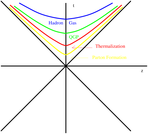
We used to think that nucleus-nucleus interaction is so complicated that the distance between the experimental data and underlying microscopic theory: QCD, is so large that we are not able to give any interpretation of the data based on QCD. My goal is to show that this wide spread opinion is just wrong. I hope to convince you that the nucleus-nucleus collisions provide such an information on the initial stage of the process, parton formation (see Fig. 1), which could be (and even has been) very essential in the disscussion of the new QCD phase: colour glass condensate (CGC).

Figure 1: The space-time picture of the ion-ion collision with the main stages of the evolution in the final state: parton formation , thermalization, Quark-Gluon Plasma (QGP) and hadron gas.

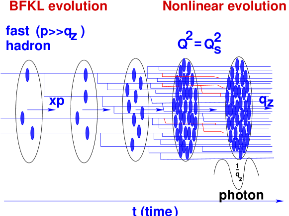
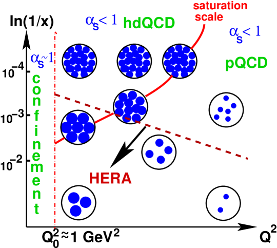
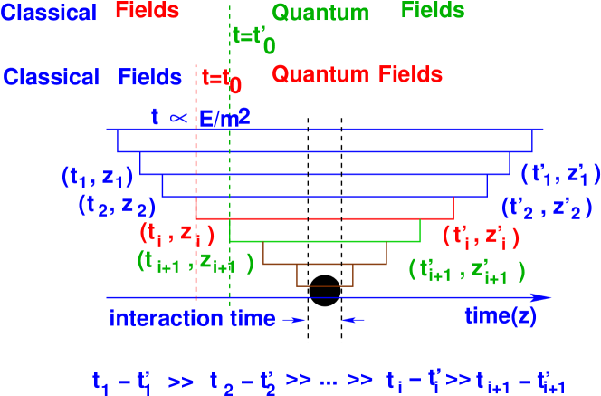
The main prediction of the CGC is the fact that the parton density in CGC region is saturated reaching a maximal valueGLR ; MUQI ; MV . The space-time picture of the QCD saturation is shown in Fig. 2. Let us consider a virtual photon, with virtuality $Q$, in the rest frame (Bjorken frame) where the photon is the standing wave which interacts with the parton (colour dipoles) with size $r\,\approx\,1/Q$. In the beginning of our process we have a small number of partons of this size but at late time the number of partons steeply increases. At some moment of time the partons start to populate densely in the proton and filled the whole proton disk (see Fig. 3).

Figure 2: Space-time picture for the deep inelastic scattering.

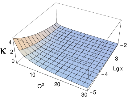
The estimate t of the value of a new scale: saturation scale which relates to the size of the parton when the partons started to populate densely (the critical curve in Fig. 3) we introduce the packing factor:

$$\mbox{P.F.}\,\,\,\equiv\,\,\,\kappa\,\,\,\,=\sigma_{parton}\,\times\,\rho\,\,\,\approx\frac{3\,\pi^{2}\alpha_{S}}{2Q^{2}_{s}(x)}\,\times\,\frac{xG(x,Q^{2}_{s}(x))}{\pi\,R^{2}}$$ (1)

The saturation scale is the solution to the equation:

$$\kappa(Q_{s}(x))\,\,=\,\,1$$ (2)

Figure 3: The distribution of partons in the transverse plane.

II Theory status

The scope of this talk does not allow us to discuss theory of the high parton density systen but, I firmly believe, that a reader should know, our approach is based on the first principles of the microscopic theory (QCD). Despites rather complicated technique, that we have to use approaching this regime, the theoretical ideas, which we based upon, are very transparent and can be easily explained and digested. For the diluted system of partons the main process is the emission of gluon and this process leads to the famous DGLAP evolution equation. However, when the density of partons increases the processes of recombination, which are proportional to the square of density ($\rho^{2}$), should enter to the game. The competition between emission ($\propto\rho$), which increases the number of partons, and recombination ($\propto\rho^{2}$), which diminishes this number, results in the equilibrium density. The phenomenon of approaching the maximal density we call ‘parton density saturation’ and the phase of QCD with saturated density is the colour glass condensate. The evolution equation which describes the saturation phenomenon is a non-linear equation GLR ; MUQI ; MV which final form was found by Balitsky and Kovchegov BK . This equation is so beautiful that I decided to present it here despites the lack of room.

$$\frac{\partial N(y,\vec{x}_{01},\vec{b})}{\partial y}\,\,=\,\frac{C_{F}\alpha_{S}}{2\pi^{2}}\,\int\,d^{2}x_{2}\,\frac{x^{2}_{01}}{x^{2}_{02}\,\,x^{2}_{12}}\,\left(2N(y,\vec{x}_{12},\vec{b}-\frac{1}{2}\vec{x}_{02})\,\right.$$ (3)

$$\left.-\,N(y,\vec{x}_{01},\vec{b})\,\,-\,\,N(y,\vec{x}_{12},\vec{b}-\frac{1}{2}\vec{x}_{02})\,N(y,\vec{x}_{02},\vec{b}-\frac{1}{2}\vec{x}_{12})\right)$$

where $x_{ij}$ are the sizes of dipoles (see Fig. 4).

Figure 4: The Balitsky-Kovchegov equation.

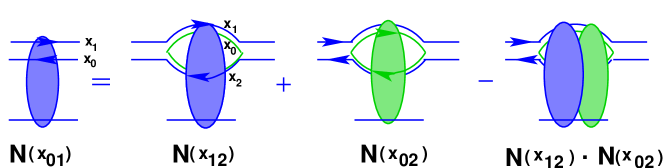
Eq. (3) shows that the degrees of freedom at high energy are the colour dipoles rather than quark and gluon themselves MUCD . The physical meaning of $N$ is the dipole-target amplitude. The equation says that the change of this amplitude from $y$ to $y+dy$ where $y=\ln t=\ln(1/x)$ and $x$ is the Bjorken variable fir DIS. is equal to the probability for the incoming dipole to decay into two dipoles. These two dipoles can interact with the target separately and simultaneously. The simultaneous interaction should be taken with the negative sign which reflects the shadowing effect or accounting for the the recombination processes.

The Balitsky-Kovchegov equation at the moment is the main theoretical tool for in many applications of the CGC dynamics despites it’s very approximate nature. It plays a role of the mean field approach in this problem.

It is very important to understand that we have a more general approach than the mean field one. This approach is based on the space-time structure of the high energy interaction in QCD (see Fig. 5). The idea of this approach is very transparent. Let us start with emission of the parton at time shown by the first dotted line in Fig. 5. All parton with high energies were created a long before this moment. The main idea MV is that these partons can be treated classically while the parton emitted at this moment can be described by QCD. Moving the moment of time (see the second dotted line in Fig. 5 we should include the gluon produced in $(t_{i},z_{i})$ into the parton system which we consider classically, but a new gluon emitted in $(t_{i+1},z_{i+1})$ shall be treated in full QCD. Since the description should be the same in these two moments ($t_{i}$ and $t_{i+1}$ we have a constraint which leads to the equation. The realization of this program is rather complicated as well as technique that is required to understand the resulting equation but the physical basis for the JIMWLK equation JIMWLK is very simple.

Figure 5: The space-time structure of high energy interaction in QCD and the renormalisation Wilson group approach (JIMWLK equation) to high parton density QCD.

The last remark that I would like to make in this brief theoretical introduction is related to the theoretical input which we will use in our description of the experimental data. It turns out that we need to know the solution to the non linear equation only in vicinity of the saturation scale together with the general understanding of the behaviour of the dipole amplitude in the saturation domain. Since the unitarity itself leads to $N\,\rightarrow\,1$ the different equations can only specify the character of approaching this maximal value. The description of the RHIC data do not depend on the details of this approaching. The behaviour near to the saturation boundary can be found just knowing the solution to the linear evolution equation.

III Comparison with the data: general approach.

I believe that the most important thing is to stipulate clearly what kind of assumptions we are making applying the general theory to an interpretation of the experimental data at accessible energies and typical distances reached by the experiment. Indeed, the theory was formulated for the dense parton system while the experimental data exist rather in the transition domain where density is not very high but not low as well. In our KLMN approachKN ; KL ; KLN ; KLM ; KLND ; KLMAZ we used three main assumptions which we will have to reformulate at the end of the talk.

1. At $x\,=\,x_{0}\,\approx\,\,10^{-1}$ we have the McLerran-Venugopalan model for the inclusive production of gluons with the saturation scale $Q^{2}_{s}(x_{0})\,\,\approx\,\,1\,GeV^{2}$ MV ;

2. The RHIC region of $x\,\approx\,10^{-3}$ is considered as the low $x$ region in which $\alpha_{S}\,\ln(1/x)\,\approx\,1$ while $\alpha_{S}\,\ll\,1$. This is not a principal assumption, but it makes the calculations much simpler and more transparent;

3. We assume that the interaction in the final state does not change significantly the distributions of particles resulting from the very beginning of the process. For hadron multiplicities, this may be a consequence of local parton hadron duality, or of the entropy conservation. Therefore multiplicity measurements are extremely important for uncovering the reaction dynamics. However, we would like to state clearly that wee do not claim that interaction in the final state are not important. We rather consider the CGC as the initial condition for the interaction in the final state.

IV Comparison with the data: HERA data.

We would like to make three statements about deep inelastic scattering data from HERA: (i) models that incorporate the parton density saturation (see for example Refs. GW ; BGK ; BGLM ; KOTE ) are able to describe the HERA data; (ii) the solution to the Balitsky-Kovchegov equation leads to the good description of the experimental data on the DIS structure functions GLMF2 ; IIM ; and (iii) the gluon structure function extracted from the fit of the experimental data is so large that the packing factors reaches the value of unity.

The set of figures illustrate this our point of view. Fig. 7 and Fig. 7 show the comparison with the experimental data the simple Golec-Biernat and Wuesthoff model in which the dipole-proton cross section is written in the form

$$\sigma(x,r_{\perp})\,\,\,=\,\,\,\sigma_{0}\,\,\left(\,\,1\,\,\,-\,\,\,\exp(\,-\,\frac{r^{2}_{\perp}}{R^{2}(x)}\,)\,\,\right)$$ (4)

with $R^{2}(x)\,\,\,=\,\,\,1/Q^{2}_{s}(x)$ , where

$$Q^{2}_{s}(x)\,\,=\,\,Q^{2}_{0}\,\left(\,\frac{x}{x_{0}}\,\right)^{-\lambda}$$ (5)

The parameters were chosen from the fit of the experimental data and they are: $\sigma_{0}$   =   23.03 mb ;   $\lambda$   =    0.288  ;   $x_{0}$   =    $3.04\,10^{-4}$;   $Q^{2}_{0}$   =   $1\,GeV^{2}$.

Figure 6: $\gamma^{*}p$ total cross sections in the Golec-Biernat and Wuesthoff model

Figure 7: DIS diffraction in the Golec-Biernat and Wuesthoff mode .

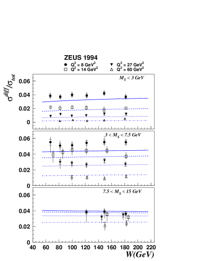
Fig. 8 gives the example how the Balitsky-Kovchegov equation is able to describe the deep inelastic structure function.

Figure 8: $F_{2}$ as result of solution to the Balitsky-Kovchegov equation. Picture is taken fron Ref. GLMF2

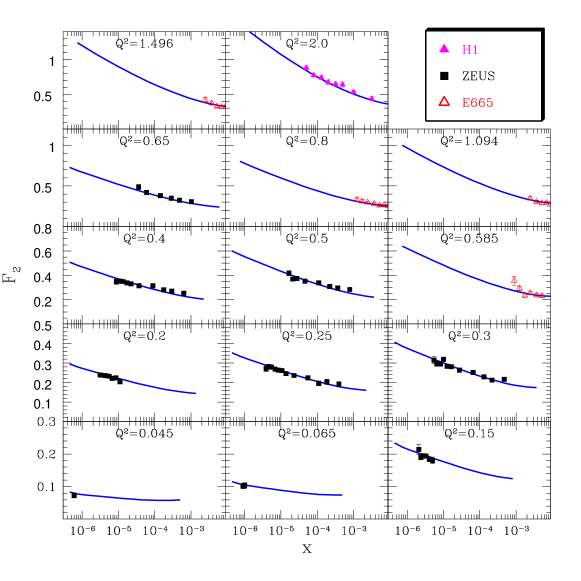
Fig. 9 gives the packing factor calculated in one of the parametrization for the extracted gluon structure function.

Figure 9: Packing factor $\kappa$ (see Eq. (1)) from the HERA data.

V Multiplicity at RHIC

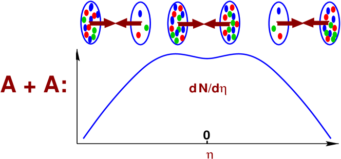
Multiplicity is the most reliable test of our approach since the third assumption is correct due to entropy conservation. The physical picture of ion-ion collision in the CGC approach is given by Fig. 10. In central region of rapidities we have a collision of two dense system of partons while in the fragmentation regions one system of partons is rather diluted while the second one turns out to be more dense than at $\eta=0$.

Figure 10: Ion-ion collision in the CGC approach.

To characterize the ion-ion collision we use several observables, namely, centrality cut, which related too typical value of the impact parameters; number of participants ($N_{part}$) , which shows the number of proton taking part in interaction; and the number of collisions ($N_{coll}$) . All these observables are discussed in details in Nardi’s talk at this conference and I will assume that you are familiar with them. Here, I only want to formulate the simple rule: if a physical observable $\propto\,\,\,N_{part}$ this observable can be described by    soft physics while observables $\propto\,\,\,N_{coll}$ are certainly related to typical hard processes, which can be treated in perturbative QCD. Soft physics at scale larger than $1\,\,GeV$ is a great surprise. In simple words the saturation in CGC is a claim that soft physics starts at $p_{t}\,\leq\,Q_{s}(x)$ and $Q_{s}$ could be large at high energies.

The key relation in the CGC is that the saturation scale is proportional to the number of participants or

$$Q^{2}_{s}(A)\,\,=\,\,\frac{3\pi^{2}}{2}\,\alpha_{S}(Q^{2}_{s})xG_{N}(x,Q^{2}_{s})\,\frac{\rho_{part}}{2}$$ (6)

and

$$S_{A}\cdot Q^{2}_{s}(A)\,\,\propto\,\,N_{part}$$ (7)

In the case of the ion-ion collisions we have actually two saturation scales in colliding ions. In the simple Golec-Biernat and Wuesthoff model they have the following dependence on energy $W$ and rapidity $y$:

$$Q^{2}_{min}\,\,=\,\,\,Q^{2}_{s}(A;W=W_{0};y=0)\,\left(\frac{W}{W_{0}}\right)^{\lambda}\,e^{-\,\lambda\,y}\,\,;$$ (8)

$$Q^{2}_{max}\,\,=\,\,\,Q^{2}_{s}(A;W=W_{0};y=0)\,\left(\frac{W}{W_{0}}\right)^{\lambda}\,e^{\lambda\,y}\,\,;$$ (9)

In our papers we use the following formula for the inclusive production GLR ; GM :

$$E{d\sigma\over d^{3}p}={4\pi N_{c}\over N_{c}^{2}-1}\ {1\over p_{t}^{2}}\ \times\,\int^{p_{t}}\,dk_{t}^{2}\,\varphi_{A_{1}}(x_{1},k_{t}^{2})\,\,\varphi_{A_{2}}(x_{2},(\vec{p}_{t}-\vec{k}_{t})^{2})$$ (10)

where $x_{1,2}=(p_{t}/\sqrt{s})\exp(\mp y)$ and $\varphi_{A_{1},A_{2}}(x,k_{t}^{2})$ is the unintegrated gluon distribution of a nucleus ( for the case of the proton one of $\varphi_{A}$ should be replace by $\varphi_{p}$.) This distribution is related to the gluon density by

$$xG(x,Q^{2})\,\,=\,\,\int^{Q^{2}}\,\,d\,k^{2}_{t}\,\varphi(x,k_{t}^{2}).$$ (11)

The multiplicity can be calculated using the following formula:

$${dN\over dy} = {1\over S}\ \ \int dp_{t}^{2}\left(E{d\sigma\over d^{3}p}\right)\,\,\,=\,\,\,{4\pi N_{c}\alpha_{S}\over N_{c}^{2}-1}\,\frac{1}{S}$$ (12)

$$\times \,\,\int{dp_{t}^{2}\over p_{t}^{2}}\ \left(\,\varphi_{A_{1}}(x_{1},p_{t}^{2})\,\,\int^{p_{t}}\,dk_{t}^{2}\ \varphi_{A_{2}}(x_{2},k_{t}^{2})\,\,+\,\,\varphi_{A_{2}}(x_{2},p_{t}^{2})\,\,\int^{p_{t}}\,dk_{t}^{2}\ \varphi_{A_{1}}(x_{1},k_{t}^{2})\,\right)$$

$$= {4\pi N_{c}\alpha_{S}\over N_{c}^{2}-1}\,\,\frac{1}{S}\,\,\int^{\infty}_{0}\,\,\frac{d\,p^{2}_{t}}{p^{4}_{t}}\,\,x_{2}G_{A_{2}}(x_{2},p^{2}_{t})\,\,x_{1}G_{A_{1}}(x_{1},p^{2}_{t})\,\,,$$

where we integrated by parts and used Eq. (11). In the KLMN treatment we assumed a simplified form of $xG$, namely,

$$xG(x;p^{2}_{t})\,\,=\,\,\left\{\begin{array}[]{l}\,\,\,\,{\kappa\over\alpha_{S}(Q^{2}_{s})}\,S\,p^{2}_{t}\,\,(1\,-\,x)^{4}\,\,\,\,p_{t}\,<\,Q_{s}(x)\,\,;\\ \\ \,\,\,\,{\kappa\over\alpha_{S}(Q^{2}_{s})}\,S\,Q^{2}_{s}(x)\,\,(1\,-\,x)^{4}\,\,\,\,p_{t}\,>\,Q_{s}(x)\,\,;\end{array}\right.$$ (16)

Inserting Eq. (16) into Eq. (12) we obtain a simple formulas:

$$\frac{dN}{dy}\,\,=\,\,Const\,\,S_{A}\,\,\,Q^{2}_{s,min}\,\ln\left(\frac{Q^{2}_{s,min}}{\Lambda^{2}_{QCD}}\right)\times\left(\,1\,\,+\,\,\frac{1}{2}\ln\left(\frac{Q^{2}_{s,min}}{Q^{2}_{s,max}}\right)\,(1-\frac{Q_{s}}{\sqrt{s}}\,e^{y})^{4}\right)$$ (17)

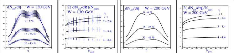
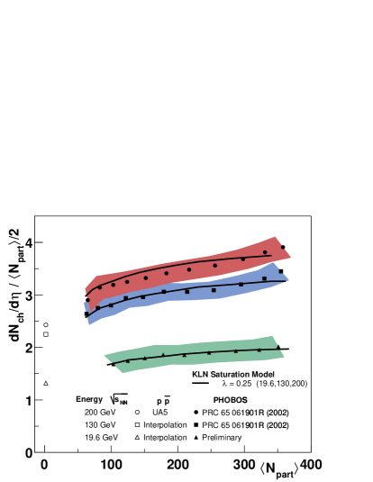
This simple formula with the saturation scales determined by Eq. (8) and Eq. (9) describes quite well the rapidity, energy and $N_{part}$ dependence of the multiplicity (see Fig. 11, Fig. 13 and Fig. 13) that have been measured at RHIC Brahms ; Phenix ; Phobos ; Star .

Figure 11: Rapidity dependence of measured multiplicity.

Figure 12: PHENIX data for $N_{part}$ dependence of the multiplicity distributions. Our calculations are labeled by ‘KLN’ in this figure.

Figure 13: PHOBOS data on energy and $N_{part}$ dependence of the multiplicity distributions. Our calculations are labeled by ‘KLN saturation model’ in this figure. $\lambda$ determines the energy and rapidity dependence of the saturation scale ( see Eq. (8) and Eq. (9))

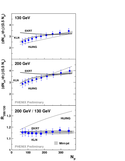
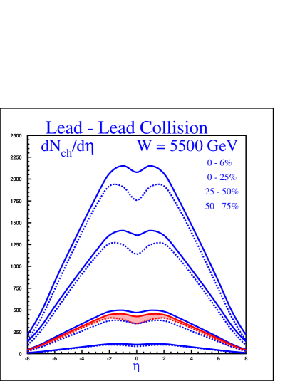
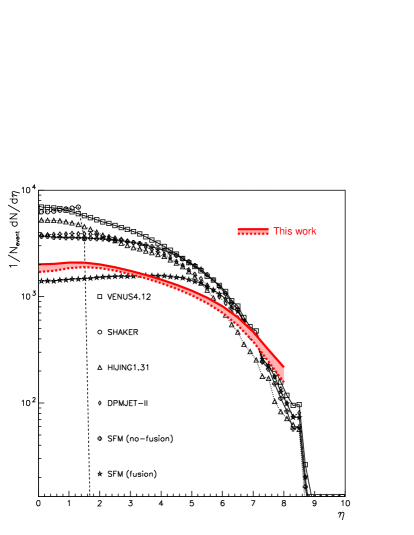
Using Eq. (17) we are able to predict the multiplicity distribution at the LHC energy KLNLHC . The systematic errors in our predictions mostly stem from the uncertainties in the energy behaviour of the saturation scale (see Ref. KLNLHC for details). The predictions are shown in Fig. 15 and Fig. 15. One can see that we expect rather low value of the multiplicity in comparison with the majority of other approaches.

Figure 14: The KLN prediction for the LHC energy. The full curves correspond the Golec-Biernat and Wuesthoff model for the energy dependence of the saturation scale. The dotted line describe the prediction if energy dependence of the saturation scale is determined by the running QCD coupling. See Ref. KLNLHC for more details.

Figure 15: Comparison our prediction with other models available on the market (see Ref. REVAP .

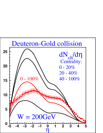
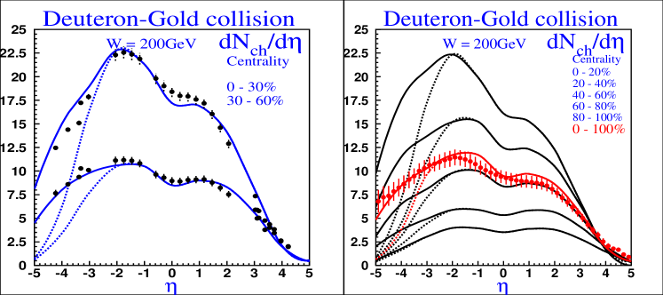
The same formula could be generalized to describe the deuteron-nucleus collisions KLND . In Fig. 16 and Fig. 17 we show our predictions for the multiplicity distribution for deuteron-gold collisions. Fig. 16 was published before RHIC data and one can see that our predictions do not agree with the experimental quite well. Therefore, we had a dilemma: the approach is not correct or some phenomenological parameters were chosen incorrectly. Fortunately, the second is the case. Indeed, we found that we have to change several parameters. It turns out that the number of participants calculated by us (see Nardi’s talk) does not agree with the number of participants that experimentalist calculated using the Glauber Monte Carlo. In new comparison we use the experimental value for $N_{part}$. Second, we treated incorrectly the events with the number of participants in the deuteron less than 1. The third change was in the value of the saturation momentum of the proton. We have to take it just the same as in the Golec-Biernat and Wuesthoff model while in our old fit we took it by 30% less. After these corrections the comparison is not bad (see Fig. 17) but we cannot describe the fragmentation region of nucleus.

Figure 16: Our prediction for the deuteron-gold collision at RHIC.

Figure 17: Our final fit of the data for the deuteron-gold collision at RHIC. The left figure for BRAUMS data while the right one for the PHONOS data

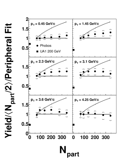
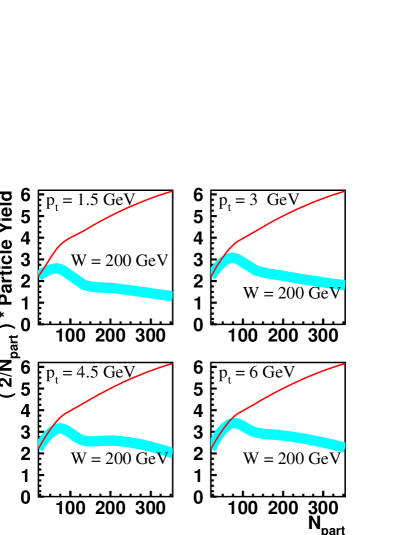
VI $N_{part}$ scaling at RHIC for ion-ion collisions

One of the most interesting results from RHIC, I believe, is so called $N_{part}$ scaling. As you can see in Fig. 19 experimental data show that $dN/dyd^{2}p_{t}\,\propto\,N_{part}$ at all values of $p_{t}$ up to $p_{t}\,\approx\,5\,GeV$. As we have discussed this fact is a strong indication that even at sufficiently large momenta the mechanism close to the ‘soft physics’ works. This scaling behaviour has a very simple explanation in the CGC approach, which is based on three observations KLM :

1. Geometrical scaling behaviour in the wide region outside of the saturation domainIIMGS : $\phi(x,p^{2}_{t})\,\,=\,\,\phi(Q^{2}_{s}(x)/p^{2}_{t})$;

2. The anomalous dimension of gluon density is $\,\,\approx\,\,\,\frac{1}{2}$ for $Q^{2}_{s}(x)\,\,\,<\,\,\,p^{2}_{t}\,\,\,<\,\,\,\frac{Q^{4}_{s}(x)}{\Lambda^{2}\,N_{part}}$;

3. For wide range of distances the saturation scale for a nuclear target    $\propto\,\,\,N_{part}\,\,\,\approx\,\,\,A^{\frac{1}{3}}$

Figure 18: $N_{part}$ scaling for gold-gold collision (PHOBOS data)

Figure 19: $N_{part}$ scaling in the CGC approach ( KLMN saturation model )KLM

The behaviour of function $\phi$ looks as it is shown in Fig. 20

Figure 20: The behaviour of functions $\phi$ for nucleus and proton in the CGC approach taking into account the anomalous dimension.

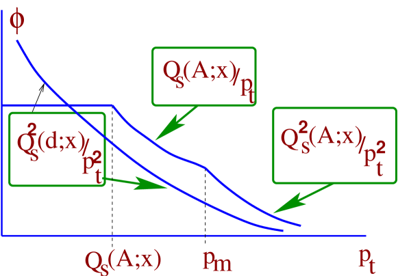
Using such $\phi$-s we obtain KLM for ion-ion collisions:

$$\frac{1}{S_{A}}E{d\sigma\over d^{3}p}\,\,\,=\,\,\,\frac{dN}{dyd^{2}p_{t}}\,\,\,\propto\,\,\,\,S_{A}Q^{2}_{s}/p^{2}_{t}\,\,\,\rightarrow\,\,\,N_{part}/p^{2}_{t}$$ (18)

More precise calculation shown in Fig. 19 lead to $N_{part}$ scaling and can describe the experimental data.

VII $N_{part}$ scaling and suppression in deuteron-nucleus collisions

Using the behaviour of functions $\phi$ shown in Fig. 20 for deuteron-nucleus collision we obtain:

$$\frac{1}{S_{A}}E{d\sigma\over d^{3}p}\,\,\,=\,\,\,\frac{dN}{dyd^{2}p_{t}}\,\,\,\propto\,\,\,S_{D}Q_{s}(A)Q_{S}(D)/p^{2}_{t}\,\,\,\rightarrow\,\,\,\sqrt{N_{part}}/p^{2}_{t}$$ (19)

Eq. (19) means that we expect a suppression in comparison with wide spread opinion that $dN/dud^{2}p_{t}$ should be proportional to $N_{part}$ KLM . The experiment shows that we do not have such a suppression in the central and nuclear fragmentation regions of rapidities but it certainly exists for forward region (see Fig. 22 and Fig. 22). The first result needs an explanation the second one is a great success of the CGC approach.

It should be stressed that the fact that the ration at $\eta=0$ and at low $p_{t}$ is much smaller than 1 itself is a strong argument in favour of the CGC since in ordinary (Glauber) approach it should be equal to unity. As far as I know there is no other explanation of this suppression.

Figure 21: Deuteron-nucleus collisions in central and nucleus fragmentation region. )

Figure 22: BRAHMS data in forward region

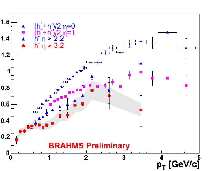
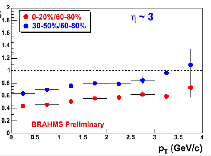
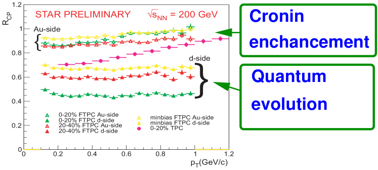
I think that the situation with a suppression is clearly illustrated by Fig. 23. In this figure one can see two clearly separated regions with quite different physics. This separation suggests the way out: for the central and nuclear fragmentation region the anomalous dimension of the gluon density is not essential while in the forward fragmentation we see the effect of quantum evolution.

Figure 23: Two different regions: Cronin enhancement due to interaction in the final state: a strong indication of the quark-gluon plasma production; and a quantum evolution region predicted bu the CGC approach KLM .

VIII Three assumptions: a new edition

However, the fact that we do not have a suppression in the range of rapidities in central and nuclear fragmentation region, makes incorrect our beautiful explanation of the $N_{part}$ scaling for ion-ion collisions. We have to assume that this scaling stems not from initial condition for our evolution but rather from strong interaction in the final state which suppress the production of the hadron from inside the nucleus. Only production from the nucleus surfaces can go out of the interacting system and can be observed. In this case we also have a $N_{part}$ scaling. Why we see this scaling up to $p_{t}\approx 5\,GeV$ ? We have not reached a clear understanding why.

I hope that you understand that we have to change our three main assumptions under the press of the experimental data. Their new edition looks as follows:

1. At $x\,>\,x_{0}\,\approx\,\,10^{-2}$ we have the McLerran-Venugopalan model for the inclusive production of gluons with the saturation scale $Q^{2}_{s}(x_{0})\,\,\approx\,\,1\,GeV^{2}$;

2. $x\,\,<\,\,x_{0}\,\approx\,\,10^{-2}$ is low $x$, i.e. $\alpha_{S}\ln(1/x)\,\,\approx\,\,1$ while $\alpha_{S}\,\,<\,\,1$;

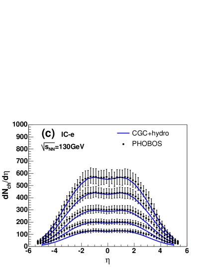
3. The CGC theory determines the initial condition for the evolution of the partonic system in ion-ion collisions. The CGC is the source of the thermalization which occurs at rather short distance of the order of $1/Q_{s}$. Our formula is CGC ( saturation) is the initial condition for hydrodynamical evolution in A + A collisions.;

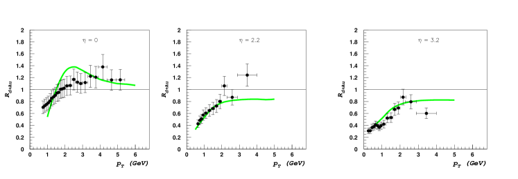
Fig. 24 shows that the CGC approach is able to describe the experimental data using these three assumptions (see Ref. KKT ).

Figure 24: The CGC approach, based on a new edition of our three assumptions, for deuteron-nucleus collisions KKT .

IX $p_{t}$ distribution: proton-proton collisions.

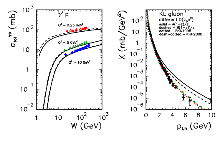
The transverse momentum distribution is a very sensitive check of the form of our input for the parton densities. In Ref. scz is shown that Eq. (16) perfectly describe the $p_{t}$ and ² distribution in proton-proton collision and DIS with the proton target (see Fig. 25).

Figure 25: $p_{t}$ and $Q^{2}$ distribution in proton - proton collisions and DIS with the proton target. Pictures are taken from Ref. scz .

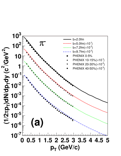
X $p_{t}$ distribution: deuteron-nucleus collisions.

In Ref. KKT it is illustrated that the CGC approach is able to describe the transverse distributions of the produced hadrons in the deuteron-nucleus collisions n(see Fig. 26. This is a powerful check of our two first assumptions as well as the simplified form of the parton densities in Eq. (16).

Figure 26: $p_{t}$ distribution in the deuteron - gold collisions in the CGC approach (see Ref. KKT ).

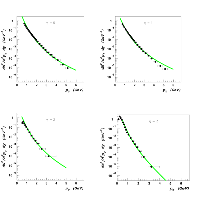
XI $p_{t}$ distribution: ion-ion collisions.

In Ref. Eskola ; Hirano the good agreement with the experimental data is achieved using the CGC theory as the initial condition for evolution which is treated in hydrodynamics (see Fig. 28 and Fig. 28). This gives a strong argument in the support of out third assumption.

Figure 27: Multiplicity distribution in CGC + hydro model of Ref.Hirano

Figure 28: $p_{t}$ distribution in CGC + hydro model of Ref. Hirano .

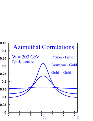
XII Azimuthal correlations

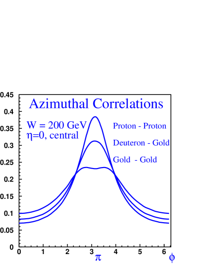
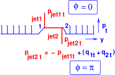
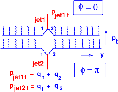
The last issue that I want to touch in this talk is the azimuthal correlations since they give a beautiful example of our expectation in the CGC approach. In the new phase-CGC, we expect decorrelations mostly because the source of the production of two particles with definite azimuthal angle between them is just independent production of two hadrons (see Fig. 32). Such a production is proportional to the square of parton density and it gives a small contribution in pQCD phase of QCD. In this phase the typical process is back-to-back correlation due to the hard rescattering of two partons that belong to the same parton shower (see Fig. 30).

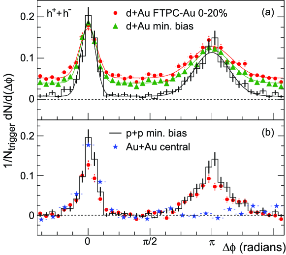
Fig. 30 and Fig. 32 show our estimates KLMAZ of the correlation in one parton shower (Fig. 30) and the resulting correlations (Fig. 32) including the production from two parton showers. Our estimates certainly reproduce the experimental data of Star collaboration ( see Fig. 33).

Figure 29: Our estimates KLMAZ of the azimuthal correlations in one partons shower for proton-proton, deuteron-gold and gold -gold collisions.

Figure 30: Picture of the strong correlation in one parton shower.

Figure 31: Our estimates KLMAZ of the azimuthal correlations in one partons shower and in two parton showers (or in other words, due to independent particle production) for proton-proton, deuteron-gold and gold -gold collisions.

Figure 32: Decorrelations in two parton showers.

Figure 33: Star data for azimuthal correlations.

XIII Resume

I hope that I convinced you that the distance between experimental data and our microscopic theory: QCD, is not so long as usually people think. The RHIC experimental data support the idea that at high parton density we are dealing with a new phase - Colour Glass Condensate. The parton density saturation, the most essential property of the CGC phase , manifests itself in the RHIC data. The most essential characteristics of the data that can be easily and elegantly described in the CGC approach are (i) energy, rapidity and centrality dependence of the particle multiplicities; (ii) the suppression of the rapidity distribution in the deuteron-nucleus collisions in comparison with the proton-proton collisions in forward region of rapidity; (iii) suppression at $\eta=0$ for rather small transverse momenta in the same data and (iv) observed azimuthal decorrelation in gold-gold collisions.

I hope that future experiments at RHIC and LHC will provide more arguments in favour of the CGC and our understanding of main features of QCD will become deeper and more transparent.

References

- (1) L. V. Gribov, E. M. Levin and M. G. Ryskin, Phys. Rep. 100 (1983) 1.
-
(2)
A.H. Mueller and J. Qiu, Nucl.Phys. B 268 (1986) 427;
J.-P. Blaizot and A.H. Mueller, Nucl. Phys. B 289 (1987) 847. - (3) L. McLerran and R. Venugopalan, Phys. Rev. D 49 (1994) 2233; 3352; D 50 (1994) 2225.
(4)
Ia. Balitsky, Nucl.Phys. B463 (1996) 99;
Yu. Kovchegov, Phys. Rev. D60 (2000) 034008. - (5) A. H. Mueller, Nucl. Phys. B415 (1994) 373; B437 (1995) 107 [arXiv:hep-ph/9408245].
(6)
J. Jalilian-Marian, A. Kovner, A. Leonidov and H. Weigert,
Phys. Rev. D59 (1999) 014014
[arXiv:hep-ph/9706377]; Nucl. Phys. B504 (1997) 415
[arXiv:hep-ph/9701284];
E. Iancu, A. Leonidov and L. D. McLerran, Phys. Lett. B510 (2001) 133 [arXiv:hep-ph/0102009]; Nucl. Phys. A692 (2001) 583 [arXiv:hep-ph/0011241];
H. Weigert, Nucl. Phys. A703 (2002) 823 [arXiv:hep-ph/0004044]. - (7) D. Kharzeev and M. Nardi, Phys. Lett. B 507 (2001) 121.
- (8) D. Kharzeev and E. Levin, Phys. Lett. B 523 (2001) 79.
- (9) D. Kharzeev, E. Levin and M. Nardi, “The onset of classical QCD dynamics in relativistic heavy ion collision hep-ph/0111315.
- (10) D. Kharzeev, E. Levin and L. McLerran, Phys. Lett. B 561 (2003) 93 [arXiv:hep-ph/0210332].
- (11) D. Kharzeev, E. Levin and M. Nardi, Nucl. Phys. A 730 (2004) 448 [arXiv:hep-ph/0212316].
- (12) D. Kharzeev, E. Levin and L. McLerran, “Jet azimuthal correlations and parton saturation in the color glass condensate,” arXiv:hep-ph/0403271.
- (13) K. Golec-Biernat and M. Wüsthoff, Phys. Rev. D59 (1999), 014017; ibid. D60 (1999), 114023; Eur. Phys. J. C20 (2001) 313.
- (14) J. Bartels, K. Golec-Biernat and H. Kowalski, Phys.Rev. D66, 014001 (2002);
- (15) J. Bartels, E. Gotsman, E. Levin, M. Lublinsky and U. Maor, Phys. Lett. B556, 114 (2003)
- (16) H. Kowalski and D. Teaney, Phys. Rev. D68,114005 (2003).
- (17) E. Gotsman, E. Levin, M. Lublinsky and U. Maor, Eur. Phys. J. C 27 (2003) 411 [arXiv:hep-ph/0209074].
- (18) E. Iancu, K. Itakura and S. Munier, Phys. Lett. B 590 (2004) 199 [arXiv:hep-ph/0310338].
- (19) E. Laenen and E. Levin, Ann. Rev. Nuc. Part. Sci. 44 (1994) 199; Yu. V. Kovchegov and D. Rischke, Phys. Rev. C56 (1997) 1084; M. Gyulassy and L. McLerran, Phys. Rev. C56 (1997) 2219; Yu. V. Kovchegov and A. H. Mueller, Nucl. Phys. B529 (1998) 451 M. A. Braun, Eur. Phys. J. C16 (2000) 337, hep-ph/0010041, hep-ph/0101070; Yu. V. Kovchegov, Phys. Rev. D64 (2000) 114016; Yu. V. Kovchegov and K. Tuchin, Phys. Rev. D65 (2002) 074026 hep-ph/0111362.
(20)
R. Debbe [BRAHMS Collaboration],
“BRAHMS results in the context of saturation and quantum evolution,”
arXiv:nucl-ex/0405018;
A. Jipa [the BRAHMS Collaboration], “Overview of the results from the BRAHMS experiment,” arXiv:nucl-ex/0404011;
M. Murray [BRAHMS Collaboration], “Scanning the phases of QCD with BRAHMS,” arXiv:nucl-ex/0404007.;
I. Arsene et al. [BRAHMS Collaboration], “On the evolution of the nuclear modification factors with rapidity and centrality in d + Au collisions at s(NN)**(1/2) = 200-GeV,” arXiv:nucl-ex/0403005;
I. Arsene et al. [BRAHMS Collaboration], “Centrality dependence of charged-particle pseudorapidity distributions from d + Au collisions at s(NN)**(1/2) = 200-GeV,” arXiv:nucl-ex/0401025;
I. Arsene et al. [BRAHMS Collaboration], Phys. Rev. Lett. 91 (2003) 072305 [arXiv:nucl-ex/0307003];
I. G. Bearden et al. [BRAHMS Collaboration], Phys. Rev. Lett. 88 (2002) 202301 [arXiv:nucl-ex/0112001];
I. G. Bearden [BRAHMS Collaboration], nucl-ex/0207006; nucl-ex/0112001; Phys. Lett. B 523, 227 (2001), nucl-ex/0108016; Phys. Rev. Lett. 87 (2001) 112305; nucl-ex/0102011; nucl-ex/0108016;
J.J. Gaardhoje et al., [ BRAHMS Collaboration ], Talk presented at the “Quark Gluon Plasma” Conference, Paris, September 2001. -
(21)
A. D. Frawley [PHENIX Collaboration],
“PHENIX highlights,”
arXiv:nucl-ex/0404009;
C. Klein-Boesing [PHENIX Collaboration], “PHENIX measurement of high particles in Au+Au and d+Au collisions at ,” arXiv:nucl-ex/0403024;
S. S. Adler et al. [PHENIX Collaboration], Phys. Rev. C 69 (2004) 034910 [arXiv:nucl-ex/0308006];
S. S. Adler et al. [PHENIX Collaboration], Phys. Rev. C 69 (2004) 034909 [arXiv:nucl-ex/0307022];
S. S. Adler et al. [PHENIX Collaboration], Phys. Rev. Lett. 91 (2003) 072303 [arXiv:nucl-ex/0306021];
S. S. Adler et al. [PHENIX Collaboration], Phys. Rev. Lett. 91 (2003) 072301 [arXiv:nucl-ex/0304022];
A. Bazilevsky [PHENIX Collaboration], nucl-ex/0209025;
A. Milov [PHENIX Collaboration], Nucl. Phys. A 698, 171 (2002), nucl-ex/0107006;
K. Adcox et al. [PHENIX Collaboration], Phys. Rev. Lett. 87, 052301 (2001), nucl-ex/0104015; Phys. Rev. Lett. 86, 3500 (2001), nucl-ex/0012008. -
(22)
B. B. Back et al. [PHOBOS Collaboration],
“Pseudorapidity dependence of charged hadron transverse momentum spectra in d
+ Au collisions at s(NN)**(1/2) = 200-GeV,”
arXiv:nucl-ex/0406017;
B. B. Back et al. [PHOBOS Collaboration], “Collision geometry scaling of Au + Au pseudorapidity density from s(NN)**(1/2) = 19.6-GeV to 200-GeV,” arXiv:nucl-ex/0405027;
B. B. Back et al. [PHOBOS Collaboration], “The landscape of particle production: Results from PHOBOS,” arXiv:nucl-ex/0405023;
R. Nouicer et al. [PHOBOS Collaboration], “Pseudorapidity distributions of charged particles in d + Au and p + p collisions at s(NN)**(1/2) = 200-GeV,” arXiv:nucl-ex/0403033;
B. B. Back et al. [PHOBOS Collaboration], “Pseudorapidity distribution of charged particles in d + Au collisions at s(NN)**(1/2) = 200-GeV,” arXiv:nucl-ex/0311009;
B. B. Back et al. [PHOBOS Collaboration], Phys. Rev. Lett. 91 (2003) 072302 [arXiv:nucl-ex/0306025];
B. B. Back et al. [PHOBOS Collaboration], Phys. Lett. B 578 (2004) 297 [arXiv:nucl-ex/0302015];
B. B. Back et al. [PHOBOS Collaboration], Phys. Rev. C 65 (2002) 061901 [arXiv:nucl-ex/0201005];
B. B. Back et al. [PHOBOS Collaboration], Phys. Rev. Lett. 87 (2001) 102303 [arXiv:nucl-ex/0106006];
B. B. Back et al. [PHOBOS Collaboration], Phys. Rev. C 65, 061901 (2002), nucl-ex/0201005; nucl-ex/0108009; Phys. Rev. Lett. 85, 3100 (2000), hep-ex/0007036;
M. D. Baker [PHOBOS Collaboration], nucl-ex/0212009. -
(23)
J. Adams et al. [STAR Collaboration],
“Azimuthal anisotropy and correlations at large transverse momenta in p + p
and Au + Au collisions at s(NN)**(1/2) = 200-GeV,”
arXiv:nucl-ex/0407007;
L. S. Barnby [STAR Collaboration], “Identified particle dependence of nuclear modification factors in d + Au collisions at RHIC,” arXiv:nucl-ex/0404027;
A. A. P. Suaide [STAR Collaboration], “High-p(T) electron distributions in d + Au and p + p collisions at RHIC,” arXiv:nucl-ex/0404019;
A. H. Tang [STAR Collaboration], “Azimuthal anisotropy and correlations in p + p, d + Au and Au + Au collisions at 200-GeV,” arXiv:nucl-ex/0403018;
J. Adams et al. [STAR Collaboration], Phys. Rev. Lett. 92 (2004) 112301 [arXiv:nucl-ex/0310004];
J. Adams et al. [STAR Collaboration], Phys. Rev. Lett. 91 (2003) 072304 [arXiv:nucl-ex/0306024]; J. Adams et al. [STAR Collaboration], Phys. Rev. Lett. 91 (2003) 172302 [arXiv:nucl-ex/0305015];
Z. b. Xu [STAR Collaboration], nucl-ex/0207019;
C. Adler et al. [STAR Collaboration], Phys. Rev. Lett. 87, 112303 (2001), nucl-ex/0106004. - (24) D. Kharzeev, E. Levin and M. Nardi, “CGC and Hadron and nucleus collisions at the LHC”.
- (25) N. Armesto and C. Pajares, Int. J. Mod. Phys. A 15 (2000) 2019 [arXiv:hep-ph/0002163].
- (26) E. Iancu, K. Itakura and L. McLerran, Nucl. Phys. A 708 (2002) 327 [arXiv:hep-ph/0203137].
- (27) D. Kharzeev, Y. V. Kovchegov and K. Tuchin, “Nuclear modification factor in d + Au collisions: Onset of suppression in the color glass condensate,” arXiv:hep-ph/0405045.
- (28) A. Szczurek, “From unintegrated gluon distributions to particle production in hadronic collisions at high energies,” arXiv:hep-ph/0309146; Acta Phys. Polon. B34 (2003) 3191 arXiv:hep-ph/0304129, B35 (2004) 161 arXiv:hep-ph/0311175.
- (29) K. J. Eskola, H. Niemi, P. V. Ruuskanen and S. S. Rasanen, Nucl. Phys. A 715 (2003) 561 [arXiv:nucl-th/0210005].
- (30) T. Hirano and Y. Nara, “Hydrodynamic afterburner for the color glass condensate and the parton energy loss,” arXiv:nucl-th/0404039.