Universal energy spectrum of tight knots and links in physics

Abstract

We argue that a systems of tightly knotted, linked, or braided flux tubes will have a universal mass-energy spectrum, since the length of fixed radius flux tubes depend only on the topology of the configuration. We motivate the discussion with plasma physics examples, then concentrate on the model of glueballs as knotted QCD flux tubes. Other applications will also be discussed.

I Introduction

It is known from plasma physics that linked magnetic flux tubes are much more stable than an unknotted single loop Moffatt:1985 . Linked flux tubes carry topological charge, and this can be thought of as a conserved (at least to lowest order) physical quantum number. Similarly, knotted flux tubes carry topological quantum numbers, and one can think of a knot as a self-linked loop. The topological charges are described by knot polynomials that are related to projections of knots or links into a plane where the crossings of the loops are assigned various attributes. Following each line around its loop generates the polynomials. Several types of polynomials have been studied in the literature (see e.g. Refs. Rolfsen ; Kauffman ): Alexander, Conway, Jones, Kauffman, etc., with increasing levels of precision for distinguishing knots. For example, the simplest knot, the trefoil, has a chiral partner (mirror image) that is not detected by the simpler polynomials, but is by the more sophisticated ones. Hence, a pair of knots with different polynomials are different, but the converse is not necessarily true. It is still an unsolved problem to find a set of polynomials that distinguishes all non-isomorphic knots/links. Similar results hold for braids, and we will also discuss these objects below.

II Review of previous physical results on tight knots and links

If the loops have fixed uniform thickness and circular cross-section (we will eventually discuss how one can relax this condition), then each knot and link has a completely specified length if the configuration is tight, i.e., is of the shortest length with the tubes undistorted and non-overlapping. If tubes have uniform cross sections, as can be approximately the case with magnetic or electric flux tubes carrying quantized flux, or for a polymer or even a piece of spaghetti, then the length of the tight knot is proportional to the mass (or energy) of the knot. This, we claim, generates a universal mass (energy) spectrum for knotted/linked configurations of objects of this type. The lengths of tight knots were not studied until the mid-1990s bio , and only recently have accurate calculations of large numbers of tight knots Rawdon and links BKPR become available. These results now make it possible to examine physical systems and compare them with the knot spectrum. The first physical example studied was tightly knotted DNA bio . More recently, we have examined the glueball spectrum of QCD Buniy:2002yx . These particles PDG are likely to be solitonic states Nielsen-Olesen that are solutions to the QCD field equations. While QCD will be our main focus in this chapter, there are many more cases where tight knots may play a role. We first proceed with an analysis of flux tubes in plasma physics. The lack of controllable quantum flux renders this case somewhat less interesting than its generalization to QCD. We will not go into any experimental details here, but we hope the experts in the areas discussed will take our general perspective into account when analyzing their data.

In order to decide if a system of flux tubes falls into the universal class of having a tight knot energy spectrum, we must first investigate the time scales involved. These are the lifetime of the soliton $\tau_{s}$ and the relaxation time $\tau_{r}$ necessary to reach the ground state of a tight knot configuration. The soliton lifetime (or the corresponding decay width $\Gamma_{s}=1/\tau_{s}$) can depend on several factors. These include the effects of flux tube breaking, rearrangement, and reconnection. The partial width for flux tube breaking is non-zero if the production of particle/anti-particle pairs is energetically possible, for example monopole/anti-monopole ($M\bar{M}$) pairs or color monopole/anti-monopole ($M_{C}\bar{M_{C}}$) pairs for magnetic flux (or color magnetic flux) or quark/anti-quark ($q\bar{q}$) pairs for color electric flux tubes. The partial widths can vary widely depending on the particle masses (e.g., $m_{q}\ll M$, so we expect $q\bar{q}$ pairs to be easier to produce than $M\bar{M}$ pairs), interaction strengths (this, for instance, enhances $M\bar{M}$ pair production versus $q\bar{q}$ pair production), and boundary conditions (tube shape and length). Rearrangement is a quantum effect where, for example, in a double donut arrangement, the loops can tunnel free of each other. Finally, reconnection is another effect where tubes break and re-attach in a different configuration. Such behavior has been seen in plasma physics, and is of major importance in understanding a variety of astrophysical systems. All these processes change topological charge, and their partial widths compete more or less favorably with each other depending on the parameters that describe the system.

III Exact calculations

While no knot lengths have been calculated exactly, it is possible to calculate the exact lengths of an infinite number of links and many braids BKPR . For links these calculations are possible in the case where each individual elements of the link lies in a plane. For braids, exact calculations are possible when the elements of the braid are either straight sections or where their centerlines follow helical paths. The shortest of all links, the double donut, is exactly calculable. The two elements lie in perpendicular planes and are tori of equal length. The shortest non–trivial braid is a helically twisted pair. “Weyl’s tube formula” is the ideal tool for calculating the volume of a flux tube Weyl ; Gray . The formula states that for a tube of constant cross-section $\sigma$ normal to a path of length $l$, the volume of the tube is just $V_{T}=l\sigma$. This is a remarkable result that holds in flat 3D. In higher dimensions or curved space, the result is more complicated, but here we need only the simple 3D case. This means that if we have an analytic form for the path and a circular cross-section we can find $V_{T}$. This leads to the fact that there is a class of exactly calculable links and braids. Since there are no known analytic forms for the path of tight knots, their volumes can only be calculated numerically, but once we have an estimate of the length, we can then also estimate the volume and therefore the energy for a corresponding physical system. Braids are also of physical interest. For the simplest example, a tightly twisted pair, the path of the center lines of such tubes are helices, and so the lengths $l(\theta_{P},h)$ depend on the pitch angle $\theta_{P}$, the radius of the tubes $r$, and the height of the braid $h$. Hence the volume is $V_{T}=2\sigma l(\theta_{P},h)$ where $\sigma=\pi r^{2}$. The volume of triple, etc., helical tight braids can also be found exactly; however, as with knots, the volumes of topologically non-trivial tight braids (those where the elements are woven together) can only be found approximately. (The helical twisted pair can also become non-trivially knotted/linked by identifying top and bottom boundaries, but we will not pursue this possibility here.) While the simple helically twisted braid has a volume that depends on the pitch angle which can potentially be adjusted by experimental conditions (see below), the tight knots and links derived from braids have no such adjustable parameter.

IV Plasma physics

Before going on to our main example of QCD, let us stop here to discuss tight links of flux in electromagnetic plasma. This example is conceptually somewhat simpler and provides motivation for what is to come.

Movement of fluids often exhibits topological properties (for a mathematical review see e.g. Ref. Arnold ). For conductive fluids, interrelation between hydro- and magnetic dynamics may cause magnetic fields, in their turn, to exhibit topological properties as well. For example, for a perfectly conducting fluid, the (abelian) magnetic helicity $\int d^{3}x\,\epsilon^{ijk}A_{i}\partial_{j}A_{k}$ is an invariant of the motion Woltier , and this quantity can be interpreted in terms of knottedness of magnetic flux lines Moffatt:1969 . Let us discuss this in some detail since its implications are central to our more general results.

IV.1 Magnetic relaxation

A perfectly conducting, viscous and incompressible fluid relaxes to a state of magnetic equilibrium without a change in topology Moffatt:1985 . The system approaches a state of magnetic equilibrium by decreasing its magnetic energy, which is achieved by contraction of the magnetic field lines. In the case of trivial topology, where field lines are unknotted and unlinked closed curves that can be contracted to a point without crossing each other, such magnetic relaxation proceeds uninterrupted. For example, the initial toroidal field configuration upon contraction deforms into a configuration of poloidal fields confined to a tube perpendicular to the original torus. Such configuration is still unstable since small disturbances augmented by the magnetic pressure lead to the increase of length of the tube and decrease of its cross-section. The relaxation eventually leads to a state with zero fields (vacuum).

If, however, the topology of the initial magnetic fields is non-trivial (for example, when flux tubes are knotted or linked), the relaxation stops when flux tubes are tightly knotted or linked. This happens because the “freeze-in” condition (see below) forces topological restrictions on possible changes in field configurations and so any initial knots and links of field lines remain topologically unchanged during relaxation. The energy of a final (equilibrium) state is determined by topology and is bounded from below. One such bound is proportional to $|{\cal H}|$, where ${\cal H}$ is the magnetic helicity (see Ref. Moffatt:1985 for details).

IV.2 Abelian helicity

Consider an abelian gauge potential 1-form $A=A_{i}dx^{i}$ and the corresponding field-strength 2-form $F=\frac{1}{2}F_{ij}dx^{i}dx^{j}$. The helicity for the field inside volume $V$ is defined by

$${\cal H}=\int_{V}AF.$$ (1)

Under a gauge transformation, $A\to A+d\psi$ and $F\to F$, and so using the Bianchi identity $dF=0$ and the Stokes theorem we find

$${\cal H}\to{\cal H}+\int_{\partial V}\psi F.$$ (2)

The helicity is thus gauge invariant if the normal component of the field $F$ vanishes on the surface $\partial V$.

It is easy to calculate the helicity for two linked flux tubes with fluxes $\Phi_{1}$ and $\Phi_{2}$. Considering first infinitely thin tubes (centered around the curves $C_{1}$ and $C_{2}$) and integrating over their cross sections we find

$${\cal H}=\Phi_{1}\int_{C_{1}}A+\Phi_{2}\int_{C_{2}}A.$$ (3)

The Stokes theorem now leads to

$${\cal H}=2n\Phi_{1}\Phi_{2},$$ (4)

where $n$ is the Gauss linking number of the two tubes (the algebraic number of times that one tube crosses the surface spanned by the other tube). It is straigtforward to generalize this to the case of linked and/or self-linked thick flux tubes.

IV.3 Non-abelian helicity

Now we begin to step toward QCD by considering a non-abelian plasma. Since both $A$ and $F$ are conserved during the plasma motion, any combination of $A$ and $F$ is a candidate for a conserved quantum number ${\cal H}$. The choice of expression is narrowed by requiring that ${\cal H}$ is a topological quantity. In particular, this requires that ${\cal H}$ be a surface integral. By analogy with the abelian case, for a conserved non-abelian helicity Jackiw:2000cd , we choose the corresponding expression with topological properties,

$${\cal H}=\int_{V}\left(AdA+\tfrac{2}{3}A^{3}\right).$$ (5)

A (time-independent) gauge transformation $A\to g^{-1}Ag+g^{-1}dg$ leads to

$${\cal H}\to{\cal H}-\tfrac{1}{3}\textrm{tr}\int_{V}\left(g^{-1}dg\right)^{3}+\textrm{tr}\int_{\partial V}gdg^{-1}A.$$ (6)

We consider only a limited set of gauge transformations such that do not change the condition $v^{\mu}A_{\mu}=0$; this implies the constraint $v^{i}\partial_{i}g=0$. Because of this constraint only two of the components $g^{-1}\partial_{i}g$ are independent and so $(g^{-1}dg)^{3}=0$. The helicity is invariant if the normal component of $A$ vanishes on the surface $\partial V$. This condition is more restrictive than the one needed in the abelian case and implies the latter.

IV.4 “Freeze-in” condition

In a perfectly conductive relativistic non-abelian plasma, the electric field vanishes in the local frame moving with the plasma. The Lorentz transformation to the rest frame gives $v^{\nu}F_{\mu\nu}=0$, where $v^{\mu}=(1,v^{i})$ is the local plasma velocity and

$$F_{\mu\nu}=\partial_{\mu}A_{\nu}-\partial_{\nu}A_{\mu}+[A_{\mu},A_{\nu}]$$ (7)

is the field strength in terms of the gauge potential $A_{\mu}$. (The equation $v^{\nu}F_{\mu\nu}=0$ is the appropriate generalization of its familiar abelian non-relativistic counterpart electrodynamics $E_{i}=\epsilon_{ijk}v^{j}B^{k}$.) In the “hydrodynamic gauge” $v^{\mu}A_{\mu}=0$, from the definition of the field strength $F_{\mu\nu}$ we obtain

$$\partial_{0}A_{i}+(\partial_{k}A_{i})v^{k}+A_{k}(\partial_{i}v^{k})=0$$ (8)

and

$$\partial_{0}F_{ij}+(\partial_{k}F_{ij})v^{k}+F_{ik}(\partial_{j}v^{k})+F_{kj}(\partial_{i}v^{k})=0.$$ (9)

As a fluid particle moves in space, the rate of change of a local quantity is given by the Lagrange derivative $d/dt=v^{\mu}\partial_{\mu}$. Applying this operator to differential forms $A=A_{i}dx^{i}$ and $F=\frac{1}{2}F_{ij}dx^{i}dx^{j}$, and using Eqs. (8), (9) and

$$(d/dt)dx^{i}=(\partial_{j}v^{i})dx^{j},$$ (10)

we find that $A$ and $F$ are constants of motion:

$$dA/dt=0,$$ (11)

$$dF/dt=0.$$ (12)

In other words, for a curve $C$ and a surface $S$ moving with the fluid, integrals $\int_{C}A$ and $\int_{S}F$ do not change in time: the magnetic lines are “frozen” into the plasma. Note the integral $\int_{C}A$ is usually called a Wilson loop in the high-energy physics literature and $\int_{S}F$ is related to the Wilson loop via Stokes’ theorem.

The freeze-in condition derived in this subsection generalizes the well-known (see e.g. Ref. electrodynamics ) “freeze-in” condition in MHD to non-abelian case. The non-relativistic analog of this result was obtained in Ref. Holm:1984yh .

V QCD and Glueballs

V.1 QCD

What is the ideal physical system in which to discover and study tight knots and links? We claim it is Quantum Chromodynamics (QCD), so in order to explain our reasoning we first pause to briefly summarize QCD PDG .

To lowest order, the standard model of particle physics can be broken into two major sectors, one describing the electroweak processes for leptons, quarks, photons and intermediate vector bosons, like electron-neutrino scattering, and the other describing the strong interactions. The electroweak processes are easier to deal with because the coupling constants of this sector are small (e.g., the fine structure constant $\alpha=e^{2}/{4\pi}$ is approximately $1/137$) so that perturbative calculations can be preformed to a high precision and are in beautiful agreement with experiment. On the other hand, the strong interactions which describes the interactions of quarks and gluons, while in principle completely described by QCD, are much more difficult to deal with because at low energy the coupling constant $\alpha_{S}={g_{S}}^{2}/{4\pi}$ is $O(1)$. This, for instance, makes the quark-antiquark ($q\bar{q}$) bound state problem analytically intractable.

In somewhat more detail, the QCD is a gauge theory with the lagrangian density

$${\cal L}=-\tfrac{1}{4}F^{a}_{\mu\nu}F^{a\mu\nu}+\bar{\psi}^{i}_{q}\gamma^{\mu}(D_{\mu})_{ij}{\psi}^{j}_{q}-m_{q}\bar{\psi}^{i}_{q}{\psi}^{i}_{q},$$ (13)

where the field strength is

$$F^{a}_{\mu\nu}=\partial_{\mu}A^{a}_{\nu}+\partial_{\nu}A^{a}_{\mu}-g_{S}f_{abc}A^{b}_{\mu}A^{c}_{\nu}$$ (14)

and the covariant derivative is

$$(D_{\mu})_{ij}=\delta_{ij}\partial_{\mu}+\tfrac{1}{2}\lambda^{a}_{ij}A^{a}_{\mu}.$$ (15)

Here the ${\psi}^{j}_{q}$s are the Dirac spinor quark fields with color ($i$) and flavor ($q$) indices, the Yang-Mills fields $A^{a}_{\mu}$ (connection) describe the gluons, the $f_{abc}$ are the structure constants for the $SU(3)$ gauge group, and the $\lambda^{a}_{ij}$’s are the triplet representation matrix elements for the quarks. Quarks come in six flavors with six associated quantum numbers conserved by the strong interactions but all except electric charge can be violated by the electroweak interactions. Color charges are confined due to the fact that $SU(3)$ is an unbroken symmetry with asymptotic freedom. I.e., the strong coupling $\alpha_{S}$ is energy dependent and becomes small at high energy but is large at low energies where it becomes $O(1)$ at a few hundred MeV. Then the theory becomes non-perturbative and confining (color charges cannot be isolated) with all observables color singlet states. These singlets are described by the quark model and are either bosonic $q\bar{q}$ bound state called mesons (pions, kaons, etc.) or fermionic $qqq$ states called baryons (protons, neutrons, etc.). Besides the mesons and baryons there are a number states that do not fit neatly into the quark model. These go by the names of hybrid states, exotic states and glueballs. Hybrid states and exotic states are thought to be unusual combinations of quarks e.g., $qq\bar{q}\bar{q}$ bosonic states, or $qqqq\bar{q}$ fermionic states, most of which have net flavor charges. The glueballs on the other hand are thought to be made of gluons with at most some virtual quark content, hence no flavor charges.

We are now in a position to support our claim that QCD is the ideal physical system in which to discover and study tight knots and links. Here are our reasons:

1. QCD is a solidly based part of the standard model of particle physics, and much about color confinement and the quark model is already well understood in this context, making much previous work transferable to the problem of tightly knotted flux tubes in this theory.

2. Unlike plasmas, fluids or other condensed matter systems where flux tubes are excitations of some media with many parameters that could hide universal behavior, flux knots in QCD can exist in the vacuum. Thus continuum states are absent and there are no media parameters to vary and obscure the universality. Hence, the results in QCD can be far less ambiguous.

3. The hadronic energy spectrum has been measured over a large range of energies (140 MeV to 10 GeV) and already many hundreds of states are known. We expect that among these, a few dozen can be classified as tightly knotted/linked flux tubes states. These states must have no valance quarks (i.e., no flavor quantum numbers) in order to be classified as glueballs.

4. Knotted solitons in QFT are already known to exist.

5. One can efficiently search for new glueball states at accelerators. (Also, data from older experiments still exist and can be reanalyzed to check the predictions of new states described below.)

V.2 Knot energies

Consider a hadronic collision that produces some number of baryons and mesons plus a gluonic state in the form of a closed QCD flux tube (or a set of tubes). From an initial state, the fields in the flux tubes quickly relax to an equilibrium configuration, which is topologically equivalent to the initial state. (We assume topological quantum numbers are conserved during this rapid process.) The relaxation proceeds through minimization of the field energy. Flux conservation and energy minimization force the fields to be homogeneous across the tube cross sections. This process occurs via shrinking the tube length, and halts to form a “tight” knot or link. The radial scale will be set by $\Lambda_{\textrm{QCD}}^{-1}$. The energy of the final state depends only on the topology of the initial state and can be estimated as follows. An arbitrarily knotted tube of radius $a$ and length $l$ has the volume $\pi a^{2}l$. Using conservation of flux $\Phi_{E}$, the energy becomes $\propto l(\textrm{tr}\Phi_{E}^{2})/(\pi a^{2})$. Fixing the radius of the tube (to be proportional to $\Lambda_{\textrm{QCD}}^{-1}$), we find that the energy is proportional to the length $l$. The dimensionless ratio $\varepsilon(K)=l/(2a)$ is a topological invariant and the simplest definition of the “knot energy” knot_energy .

Table 1: Comparison between the glueball mass spectrum and knot energies.

State	Mass	$K$	$\varepsilon(K)$	$E(G)$
$f_{0}(600)$	$400-1200$	$2^{2}_{1}$	$12.6\ [4\pi]$	$768\ [766]$
$f_{0}(980)$	$980\pm 10$	$3_{1}$	$16.4$	$993$
$f_{2}(1270)$	$1275.4\pm 1.2$	$2^{2}_{1}*0_{1}$	$[6\pi+2]$	$[1256]$
$f_{1}(1285)$	$1281.9\pm 0.6$	$4_{1}$	$21.2$	$1277$
		$4^{2}_{1}$	$(21.4)$	$(1289)$
$f_{1}(1420)$	$1426.3\pm 1.1$	$5_{1}$	$24.2$	$1454$
$\{f_{2}(1430)$	$\approx 1430\}$	$5_{1}$	$24.2$	$1454+\delta^{\prime}$
$f_{0}(1370)$	$1200-1500$	$3_{1}*0_{1}$	$(24.7)$	$(1484)$
$f_{0}(1500)$	$1507\pm 5$	$5_{2}$	$24.9$	$1496$
$\{f_{1}(1510)$	$1518\pm 5\}$	$5_{2}$	$24.9$	$1496+\delta$
$f^{\prime}_{2}(1525)$	$1525\pm 5$	$5_{2}$	$24.9$	$1496+3\delta$
$\{f_{2}(1565)$	$1546\pm 12\}$	$5^{2}_{1}$	$(25.9)$	$(1555)$
$\{f_{2}(1640)$	$1638\pm 6\}$	$6^{3}_{3}$	$((27.3))$	$((1638))$
..
		$(2^{2}_{1}*0_{1})*0_{1}$	$[8\pi+3]$	$[1686]$
$f_{0}(1710)$	$1713\pm 6$	$6^{3}_{2}$	$((28.6))$	$((1714))$
		$3_{1}\#3_{1}^{*}$	$28.9\ (30.5)$	$1732\ (1827)$
		$3_{1}\#3_{1}$	$29.1\ (30.5)$	$1744\ (1827)$
		$2^{2}_{1}*2^{2}_{1}$	$[8\pi+4]$	$[1745]$
		$6_{2}$	$29.2$	$1750$
		$6_{1}$	$29.3$	$1756$
		$6_{3}$	$30.5$	$1827$
		$7_{1}$	$30.9$	$1850$
		$8_{19}$	$31.0$	$1856$
		$8_{20}$	$32.7$	$1957$
$f_{2}(2010)$	$2011^{+60}_{-80}$	$7_{2}$	$33.2$	$1986$
$f_{4}(2050)$	$2025\pm 8$	$8_{21}$	$33.9$	$2028$
		$8_{1}$	$37.0$	$2211$
		$10_{161,162}$	$37.6$	$2247$
$f_{2}(2300)$	$2297\pm 28$	$8_{18}$, $9_{1}$	$38.3$	$2288$
$f_{2}(2340)$	$2339\pm 60$	$9_{2}$	$40.0$	$2389$
		$10_{1}$	$44.8$	$2672$
		$11_{1}$	$47.0$	$2802$

Many knot energies have been calculated by Monte Carlo methods bio and certain types can be calculated exactly (see below), while for other cases simple estimates can be made (see Table 1). For example, the knot energy of the connected product of two knots $K_{1}$ and $K_{2}$ satisfies

$$\varepsilon(K_{1}\#K_{2})<\varepsilon(K_{1})+\varepsilon(K_{2}).$$ (16)

A rule of thumb is

$$\varepsilon(K_{1}\#K_{2})\approx\varepsilon(K_{1})+\varepsilon(K_{2})-(2\pi-4).$$ (17)

Most of the knot energies in Table 1 have been taken from Ref. bio , but we have independently calculated the energy of $2^{2}_{1}$, $4^{3}_{1}$ and $6^{4}_{1}$ exactly and the energy for several other knots and links approximately. We find $\varepsilon(2^{2}_{1})=4\pi\approx 12.57$, to be compared with the Monte Carlo value $12.6$. We also find $\varepsilon(4^{3}_{1})=6\pi+2$ and $\varepsilon(6^{4}_{1})=8\pi+3$, where there are no Monte Carlo comparisons available, or needed. Other exactly calculable links can be found in Ref. BKPR and an example of a link with energy $10\pi+5$ is shown in Fig. 1.

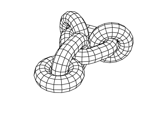
Figure 1: An example of an exactly calculable link.

V.3 Model

In our model, the chromoelectric fields $F_{0i}$ are confined to knotted/linked tubes. After an initial time evolution, the system reaches a static equilibrium state which is described by the energy density

$${{\mathcal{E}}}_{E}=\tfrac{1}{2}\textrm{tr}F_{0i}F^{0i}-V.$$ (18)

Similar to the MIT bag model MIT-bag , we have included a constant potential energy $V$ needed to keep the tubes at a fixed cross-section. The chromoelectric flux $\Phi_{E}$ is conserved and we assume flux tubes carry one flux quantum. To account for conservation of the flux, we add to Eq. (18) the term

$$\textrm{tr}\lambda\{\Phi_{E}/(\pi a^{2})-n^{i}F_{0i}\},$$ (19)

where $n^{i}$ is the normal vector to a section of the tube and $\lambda$ is a Lagrange multiplier. The energy density should be constant under variations of the degrees of freedom, the gauge potentials $A_{\mu}$. This leads to the system of equations

$$D^{0}(F_{0i}-\lambda n_{i})=0,$$ (20)

$$D^{i}(F_{0i}-\lambda n_{i})=0,$$ (21)

which has the constant field

$$F_{0i}=(\Phi_{E}/\pi a^{2})n_{i}$$ (22)

as its solution. With this solution, the energy is positive and proportional to $l$ and thus the minimum of the energy is achieved by shortening $l$, i.e., tightening the knot.

The case of chromomagnetic flux tubes can be similarly considered. This requires the confinement of color magnetic flux tubes which is possible if there are light quarks in the spectrum of the theory Goldhaber:1999sj .

Lattice calculations, QCD sum rules, electric flux tube models, and constituent glue models agree that the lightest non–$q\bar{q}$ states are glueballs with quantum numbers $J^{++}=0^{++}$ and $2^{++}$ (see Ref. West ). We will model all $J^{++}$ states (i.e., all $f_{J}$ and $f^{\prime}_{J}$ states listed by the PDG PDG ), some of which will be identified with rotational excitations, as knotted/linked chromoelectric QCD flux tubes. We proceed to identify knotted and linked QCD flux tubes with glueballs, where we include all $f_{J}$ and $f^{\prime}_{J}$ states. The lightest candidate is the $f_{0}(600)$, which we identify with the shortest knot/link, i.e., the $2^{2}_{1}$ link; the $f_{0}(980)$ is identified with the next shortest knot, the $3_{1}$ trefoil knot, and so forth. All knot and link energies have been calculated for states with energies less then $1680\,\textrm{MeV}$. Above $1680\,\textrm{MeV}$ the number of knots and links grows rapidly, and few of their energies have been calculated. However, we do find knot energies corresponding to all known $f_{J}$ and $f^{\prime}_{J}$ states, and so can make preliminary identifications in this region. (We focus on $f_{J}$ and $f^{\prime}_{J}$ states from the PDG summary tables. The experimental errors are also quoted from the PDG. There are a number of additional states reported in the extended tables, but some of this data is either conflicting or inconclusive.)

Our detailed results are collected in Table 1, where we list $f_{J}$ and $f^{\prime}_{J}$ masses, our identifications of these states with knots and the corresponding knot energies.

Figure 2: Relationship between the glueball spectrum $E(G)$ and knot energies $\varepsilon(K)$. Each point in this figure represents a glueball identified with a knot or link. The straight line is our model and is drawn for the fit (23).

Figure 3: The same as in Fig. 2, but the first glueball is missed out.

Figure 4: The same as in Fig. 2, but the first knot/link is missed out.

In Fig. 2 we compare the mass spectrum of $f_{J}$ states with the identified knot and link energies. Since errors for the knot energies in Ref. bio were not reported, we conservatively assumed the error to be $1\%$. A least squares fit to the most reliable data (below $1680\,\textrm{MeV}$) gives

$$E(G)=(23.4\pm 46.1)+(59.1\pm 2.1)\varepsilon(K)\ \ \ [\textrm{MeV}],$$ (23)

with $\chi^{2}=9.1$. The data used in this fit is the first seven $f_{J}$ states (filled circles in Fig. 2) in the PDG summary tables. Inclusion of the remaining seven (non-excitation) states (unfilled circles in Fig. 2) in Table 1, where either the glueball or knot energies are less reliable, does not significantly alter the fit and leads to

$$E(G)=(26.9\pm 24.9)+(58.9\pm 1.0)\varepsilon(K)\ \ \ [\textrm{MeV}],$$ (24)

with $\chi^{2}=10.1$. The fit (23) is in good agreement with our model, where $E(G)$ is proportional to $\varepsilon(K)$. Better HEP data and the calculation of more knot energies will provide further tests of the model and improve the high mass identification.

For comparison, we have fitted the same data in Fig. 3 except that the first glueball is missed out; this results in $\chi^{2}=231$. Similarly, we have fitted the same data in Fig. 4 except that this time the first link is missed out; this results in $\chi^{2}=355$. This is strong evidence that our identification is appropriate.

In terms of the bag model MIT-bag , the interior of tight knots correspond to the interior of the bag. The flux through the knot is supported by current sheets on the bag boundary (surface of the tube). Knot complexity can be reduced (or increased) by unknotting (knotting) operations Rolfsen ; Kauffman . In terms of flux tubes, these moves are equivalent to reconnection events reconnection . Hence, a metastable glueball may decay via reconnection. Once all topological charge is lost, metastability is lost, and the decay proceeds to completion. Two other glueball decay processes are: flux tube (string) breaking; this favors large decay widths for configurations with long flux tube components; and quantum fluctuations that unlink flux tubes; this would tend to broaden states with short flux tube components. As yet we are not able to go beyond providing a phenomenological fit to these qualitative observations Buniy:2002yx , but hope to be able to do so in the future.

We have assumed one fluxoid per tube. There may be states with more than one fluxoid, but these would presumably have somewhat fatter flux tubes with higher flux densities and higher energies. For example, the two fluxoid trefoil knot $3_{1}$ would certainly have $\varepsilon(K)>2\,\varepsilon(3_{1})$ and a fairly reliable estimate gives $\varepsilon(K)\approx 2\sqrt{2}\,\varepsilon(3_{1})$. Hence most multifluxoid states would be above the mass range of known glueball candidates.

VI Discussion and conclusions

We expect all tight knots and links to be described by smooth curves with minimum radius of curvature $2r$ where $r$ is the tube radius. Consider how we would approximate such a curve on a square lattice. The simplest nontrivial example is the double donut. We consider one of its loops (a circle) which we call $\Gamma$ to be centered on a particular lattice point $P$. The radius of the circle $R$ is some number of lattice spacings away from $P$ (we assume we are in a lattice plane), along the direction of one of $P$’s nearest neighbors. Assume all other points on $\Gamma$ are at a distance $d\geq R$ away from $P$. If we minimize the length $L$ of $\Gamma$, then the ratio of $L$ to the circumference of a circle of radius $R$ is

$$\frac{L_{\textrm{min}}}{2\pi R}=4/\pi,$$ (25)

which is the best approximation (about a 27% error) we can have on a square lattice. Similar arguments show we can do somewhat better on a hexagonal lattice where we can achieve

$$\frac{L_{\textrm{min}}}{2\pi R}=2\sqrt{3}/\pi,$$ (26)

about a 10% error. However, neither of these approximations are stunningly successful, nor does decreasing the lattice spacing improve the approximations. We assume other knots and links will be approximated on the lattice with similar accuracy. It is interesting to note here that both lattice estimates are too high and that lattice QCD typically predicts glueball masses above 1 GeV, while Monte Carlo predictions for tight knots leads to a lighter glueball spectrum with lightest state just below 800 MeV. Lattice QCD are certainly more sophisticated and involved than the simple estimates we have just made, but we do expect requiring knots/links to lie on a lattice to give glueball masses on the high side. Furthermore, the tube cross section on a lattice is not circular, inhibiting tight packing, and the amount of curvature energy on the lattice is likely to be more than for a smooth curve. We expect these effect to also contribute to increasing the lattice glueball mass estimates.

Let us return to continuum physics and consider a slab of material that can support flux tubes. We have in mind a superfluid or superconductor, but are not limited to these possibilities. Assume further that the flux tubes carry one and only one unit of flux. Next consider manipulating these flux tubes. For instance, consider a hypothetical superconductor where the flux tubes are pinned at the bottom of the slab, say by being attracted to the poles of some magnetic material, and at the top of the slab they are each associated with the pole of a movable permanent magnet, perhaps a magnetic whisker, or fine solenoid. If the north poles of a flux tube is on the top surface, we call it a ($+$) flux tube (and ($-$) for the south pole at the top). Since the flux tubes are pinned on the bottom of the slab we can maneuver the top ends into a braid. For example, if there are two flux tubes we can rotate them around each other to make a helically twisted pair. If there are three or more flux tubes we can twist them or braid them. If we measure the forces on the magnets when the flux tubes are being manipulated and use these to find the energy needed to form a braided configuration, then we gain information on the tension of the flux tubes and on the energy stored in a tight braid. If we have both ($+$) and ($-$) flux tubes we can bring ($+$) – ($-$) pairs together, annihilate the ends so the tube can be pulled into the interior of the superconductor. If we do this at both the top and bottom surfaces for a braided pair then it should be possible to form a bulk knot (similar for links). Assuming they have time to relax to tight configurations, the energy released by the eventual decay of these structures in the bulk should correspond to the universal energy spectrum described above. Perhaps there is no system with all the properties of our ideal superconductor; however, there are systems that contain many if not most of the desired features.

Another collection of physical systems of potential interest for its ability to support vortices, and so knots and braids, are the atomic Bose-Einstein condensates. For example, dilute ⁸⁷Rb atoms at $80\ \textrm{nK}$. Recently results have been presented demonstrating laser stirring of these condensates to produce vortices BEC . As many as seven vortices have been seen in a $0.1\ \textrm{mm}^{2}$ region. One could hope that advancement in these techniques could lead to more complicated solitonic structures, in particular knots, links, and braids. The advantage of these systems is the experimental accessibility of these structures, and the large percentage of the volume of the system taken up by the solitons. This could potentially dramatically improve the signal-to-noise ratio in the study of tight knots in condensed matter systems.

We have argued that knotted/linked solitonic physical systems have universal mass-energy spectra and have demonstrated this with a detailed example from QCD. We have provided other examples that are good candidates but where the universality has yet to be seen. A system is a candidate if it contains line solitons that can (somewhat paradoxically) relax to their tight knot/link ground state in a time shorter than their decay time. Future work along these lines could tie knot theory to many subfields of physics or to other sciences.

References

- (1) H. K. Moffatt, J. Fluid Mech. 159, 359 (1985).
- (2) D. Rolfsen, Knots and Links, Publish or Perish, 1990.
- (3) L. H. Kauffman, Knots and Physics, World Scientific, 2001.
- (4) V. Katritch, et al., Nature 384, 142 (1996); V. Katritch, et al., Nature 388, 148 (1997).
- (5) K. Millett and E. Rawdon, J. of Comp. Phys. 186, 426 (2003).
- (6) R. V. Buniy, T. W. Kephart, M. Piatek and E. Rawdon, in preparation.
- (7) R. V. Buniy and T. W. Kephart, Phys. Lett. B 576, 127 (2003).
- (8) K. Hagiwara et al., Phys. Rev. D 66, 010001 (2002).
- (9) H. B. Nielsen and P. Olesen, Nucl. Phys. B 61, 45 (1973).
- (10) H. Weyl, Am. J. Math. 61, 461 (1939).
- (11) A. Gray, Tubes, Addison-Wesley, 1990.
- (12) V. I. Arnold and B. A. Khesin, Topological Methods in Hydrodynamics, Springer, 1998.
- (13) L. Woltier, Proc. Nat. Acad. Sci. 44, 489 (1958).
- (14) H. K. Moffatt, J. Fluid Mech. 35, 117 (1969).
- (15) R. Jackiw, V. P. Nair, and So-Young Pi, Phys. Rev. D 62, 085018 (2000).
- (16) L. D. Landau and E. M. Lifshitz, Electrodynamics of Continuous Media, Pergamon Press, 1984.
- (17) D. D. Holm and B. A. Kupershmidt, Phys. Rev. D 30, 2557 (1984).
- (18) H. K. Moffatt, Nature 347, 367 (1990); S. G. Whittington, D. W. Sumners, and T. Lodge, editors, Topology and Geometry in Polymer Science, Springer, 1998; R. A. Litherland, J. Simon, O. Durumeric, and E. Rawdon, Topology Appl. 91, 233 (1999); G. Buck and J. Simon, Topology Appl. 91, 245 (1999).
- (19) A. Chodos, R. L. Jaffe, K. Johnson, Charles B. Thorn, and V. F. Weisskopf, Phys. Rev. D 9, 3471 (1974); T. DeGrand, R. L. Jaffe, K. Johnson, and J. E. Kiskis, Phys. Rev. D 12, 2060 (1975).
- (20) A. S. Goldhaber, Phys. Rept. 315, 83 (1999).
- (21) For further discussion of glueballs and their quantum numbers see, for instance G. B. West, Nucl. Phys. Proc. Suppl. 54A, 353 (1997); N. A. Tornqvist, arXiv:hep-ph/9510256; J. Terning, arXiv:hep-ph/0204012; R. C. Brower, Int. J. Mod. Phys. A16S1C, 1005 (2001); M. Suzuki, Phys. Rev. D 65, 097507 (2002); M. Teper, Nucl. Phys. Proc. Suppl. 109, 134 (2002).
- (22) E. Priest and T. Forbes, Magnetic Reconnection: MHD Theory and Applications, Cambridge University Press, 2000.
- (23) M. Matthews at al., Phys. Rev. Lett. 83, 2498 (1999); K. Madison at al., Phys. Rev. Lett. 84, 806 (2000).