CERN-PH-TH/2004-146

TUM-HEP-556/04

hep-ph/0408016

Waiting for the Discovery of $B^{0}_{d}\to K^{0}\bar{K}^{0}$

Robert Fleischer^a and Stefan Recksiegel^b

^a Theory Division, Department of Physics, CERN, CH-1211 Geneva 23, Switzerland

^b Physik Department, Technische Universität München, D-85748 Garching, Germany

The CP asymmetries of the decay $B_{d}^{0}\to K^{0}\bar{K}^{0}$, which originates from $\bar{b}\to\bar{d}s\bar{s}$ flavour-changing neutral-current processes, and its CP-averaged branching ratio BR$(B_{d}\to K^{0}\bar{K}^{0})$ offer interesting avenues to explore flavour physics. We show that we may characterize this channel, within the Standard Model, in a theoretically clean manner through a surface in observable space. In order to extract the relevant information from BR$(B_{d}\to K^{0}\bar{K}^{0})$, further information is required, which is provided by the $B\to\pi\pi$ system and the $SU(3)$ flavour symmetry, where we include the leading factorizable $SU(3)$-breaking corrections and discuss how experimental insights into non-factorizable effects can be obtained. We point out that the Standard Model implies a lower bound for BR$(B_{d}\to K^{0}\bar{K}^{0})$, which is very close to its current experimental upper bound, thereby suggesting that this decay should soon be observed. Moreover, we explore the implications for “colour suppression” in the $B\to\pi\pi$ system, and convert the data for these modes into a peculiar Standard-Model pattern for the CP-violating $B_{d}^{0}\to K^{0}\bar{K}^{0}$ observables.

August 2004

1 Setting the Stage

The $B$ factories allow us to confront the Kobayashi–Maskawa (KM) mechanism of CP violation [1], which describes this phenomenon in the Standard Model (SM), with a steadily increasing amount of experimental data (for a recent overview, see [2]). An interesting element of this programme is the decay $B_{d}^{0}\to K^{0}\bar{K}^{0}$. It originates from $\bar{b}\to\bar{d}s\bar{s}$ flavour-changing neutral-current (FCNC) processes, which are governed by QCD penguin diagrams in the SM. Should these topologies be dominated by internal top-quark exchanges, the CP asymmetries of $B_{d}^{0}\to K^{0}\bar{K}^{0}$ would vanish in the SM thanks to a subtle cancellation of weak phases, thereby suggesting an interesting test of the KM mechanism (see, for instance, [3]). However, contributions from penguins with internal up- and charm-quark exchanges are expected to yield sizeable CP asymmetries in $B_{d}^{0}\to K^{0}\bar{K}^{0}$ even within the SM, so that the interpretation of these effects is much more complicated [4]. In view of the impressive progress since these early studies of $B_{d}^{0}\to K^{0}\bar{K}^{0}$, and the strong experimental upper bound for the corresponding CP-averaged branching ratio [5],

$$\mbox{BR}(B_{d}\to K^{0}\bar{K}^{0})\equiv\frac{\mbox{BR}(B_{d}^{0}\to K^{0}\bar{K}^{0})+\mbox{BR}(\bar{B}_{d}^{0}\to K^{0}\bar{K}^{0})}{2}<1.5\times 10^{-6}\,\,\mbox{(90\% C.L.)},$$ (1)

it is interesting to return to this decay.

As usual, we consider the following time-dependent rate asymmetry:

$$\frac{\Gamma(B^{0}_{d}(t)\to K^{0}\bar{K}^{0})-\Gamma(\bar{B}^{0}_{d}(t)\to K^{0}\bar{K}^{0})}{\Gamma(B^{0}_{d}(t)\to K^{0}\bar{K}^{0})+\Gamma(\bar{B}^{0}_{d}(t)\to K^{0}\bar{K}^{0})}$$ (2)

$$={\cal A}_{\rm CP}^{\rm dir}(B_{d}\to K^{0}\bar{K}^{0})\cos(\Delta M_{d}t)+{\cal A}_{\rm CP}^{\rm mix}(B_{d}\to K^{0}\bar{K}^{0})\sin(\Delta M_{d}t),$$

where ${\cal A}_{\rm CP}^{\rm dir}(B_{d}\to K^{0}\bar{K}^{0})$ and ${\cal A}_{\rm CP}^{\rm mix}(B_{d}\to K^{0}\bar{K}^{0})$ describe the direct and mixing-induced CP asymmetries, respectively. In order to analyse these observables, we have to parametrize the $B_{d}^{0}\to K^{0}\bar{K}^{0}$ decay amplitude appropriately. Within the SM, we may write

$$A(B_{d}^{0}\to K^{0}\bar{K}^{0})=\lambda^{(d)}_{u}{\cal P}_{u}^{K\!K}+\lambda^{(d)}_{c}{\cal P}_{c}^{K\!K}+\lambda^{(d)}_{t}{\cal P}_{t}^{K\!K},$$ (3)

where the $\lambda^{(d)}_{q}\equiv V_{qd}V_{qb}^{\ast}$ are CKM factors, and the ${\cal P}_{q}^{K\!K}$ denote the strong amplitudes of penguin topologies with internal $q$-quark exchanges, which receive tiny contributions from colour-suppressed electroweak (EW) penguins and are fully dominated by QCD penguin processes. If we now eliminate $\lambda^{(d)}_{t}$ with the help of the relation

$$\lambda^{(d)}_{t}=-\lambda^{(d)}_{u}-\lambda^{(d)}_{c},$$ (4)

which follows from the unitarity of the Cabibbo–Kobayashi–Maskawa (CKM) matrix, and use the Wolfenstein parametrization [6], we obtain

$$A(B^{0}_{d}\to K^{0}\bar{K}^{0})=\lambda^{3}A{\cal P}_{tc}^{K\!K}\left[1-\rho_{K\!K}e^{i\theta_{K\!K}}e^{i\gamma}\right],$$ (5)

where ${\cal P}_{tc}^{K\!K}\equiv{\cal P}_{t}^{K\!K}-{\cal P}_{c}^{K\!K}$, and

$$\rho_{K\!K}e^{i\theta_{K\!K}}\equiv R_{b}\left[\frac{{\cal P}_{t}^{K\!K}-{\cal P}_{u}^{K\!K}}{{\cal P}_{t}^{K\!K}-{\cal P}_{c}^{K\!K}}\right],$$ (6)

with

$$R_{b}\equiv\left(1-\frac{\lambda^{2}}{2}\right)\frac{1}{\lambda}\left|\frac{V_{ub}}{V_{cb}}\right|=\sqrt{\bar{\varrho}^{2}+\bar{\eta}^{2}}=0.37\pm 0.04.$$ (7)

Applying the standard formalism to deal with the CP-violating observables provided by (2) [2], we straightforwardly arrive at

$${\cal A}_{\rm CP}^{\rm dir}\equiv{\cal A}_{\rm CP}^{\rm dir}(B_{d}\to K^{0}\bar{K}^{0})=\frac{2\rho_{K\!K}\sin\theta_{K\!K}\sin\gamma}{1-2\rho_{K\!K}\cos\theta_{K\!K}\cos\gamma+\rho_{K\!K}^{2}}$$ (8)

$${\cal A}_{\rm CP}^{\rm mix}\equiv{\cal A}_{\rm CP}^{\rm mix}(B_{d}\to K^{0}\bar{K}^{0})=\frac{\sin\phi_{d}-2\rho_{K\!K}\cos\theta_{K\!K}\sin(\phi_{d}+\gamma)+\rho_{K\!K}^{2}\sin(\phi_{d}+2\gamma)}{1-2\rho_{K\!K}\cos\theta_{K\!K}\cos\gamma+\rho_{K\!K}^{2}},$$ (9)

where the $B^{0}_{d}$–$\bar{B}^{0}_{d}$ mixing phase $\phi_{d}$ agrees with $2\beta$ in the SM; $\beta$ and $\gamma$ are the usual angles of the unitarity triangle of the CKM matrix.

The outline of this paper is as follows: in Section 2, we show that $B^{0}_{d}\to K^{0}\bar{K}^{0}$ can be efficiently characterized in the SM through a surface in the three-dimensional space of its observables. In order to extract the relevant information from the CP-averaged branching ratio, an additional input is needed, which is offered by the $B\to\pi\pi$ system and the $SU(3)$ flavour symmetry. We show how insights into non-factorizable $SU(3)$-breaking effects in the relevant hadronic penguin amplitudes can be obtained, and point out that the current $B$-factory data are consistent with small corrections, although the experimental uncertainties are still large. One of the main results of our analysis are lower bounds for BR$(B_{d}\to K^{0}\bar{K}^{0})$, which are remarkably close to the experimental upper bound in (1), thereby suggesting that this decay should be observed in the near future at the $B$ factories. In Section 3, we demonstrate then that the measurement of the $B_{d}\to K^{0}\bar{K}^{0}$ observables will allow us to reveal the hadronic substructure of the $B\to\pi\pi$ system, providing in particular insights into the issue of “colour suppression”. Conversely, using the pattern of the current $B$-factory data as a guideline, we calculate allowed regions in the space of the CP-violating $B_{d}\to K^{0}\bar{K}^{0}$ observables within the SM, which may be helpful in the future to search for new-physics (NP) contributions to $\bar{b}\to\bar{d}s\bar{s}$ FCNC processes. Finally, we summarize our conclusions in Section 4.

2 Standard-Model Picture of $B^{0}_{d}\to K^{0}\bar{K}^{0}$

2.1 Preliminaries: Top-Quark Dominance

It is instructive to have first a brief look at the case of top-quark dominance, where (6) simplifies as follows:

$$\rho_{K\!K}e^{i\theta_{K\!K}}=R_{b}.$$ (10)

Since the CP-conserving strong phase $\theta_{K\!K}$ vanishes in this expression, (8) implies that the direct CP asymmetry of $B_{d}\to K^{0}\bar{K}^{0}$ vanishes as well. The analysis of the mixing-induced CP asymmetry (9) is a bit more complicated. If we take into account that we have $\phi_{d}=2\beta$ in the SM, and use the relations

$$\sin\beta=\frac{\bar{\eta}}{\sqrt{(1-\bar{\varrho})^{2}+\bar{\eta}^{2}}},\quad\cos\beta=\frac{1-\bar{\varrho}}{\sqrt{(1-\bar{\varrho})^{2}+\bar{\eta}^{2}}}$$ (11)

$$\sin\gamma=\frac{\bar{\eta}}{\sqrt{\bar{\varrho}^{2}+\bar{\eta}^{2}}},\quad\cos\gamma=\frac{\bar{\varrho}}{\sqrt{\bar{\varrho}^{2}+\bar{\eta}^{2}}}$$ (12)

between the angles of the unitarity triangle and the Wolfenstein parameters [6], we may show that ${\cal A}_{\rm CP}^{\rm mix}$ would actually also vanish. This can be seen more transparently if we eliminate $\lambda^{(d)}_{u}$ instead of $\lambda^{(d)}_{t}$ in (3). Assuming then top-quark dominance, we obtain a cancellation between the weak phase $\beta$ of $\lambda^{(d)}_{t}$ and the $\beta$ introduced through the SM value of $\phi_{d}$, thereby yielding a vanishing mixing-induced $B^{0}_{d}\to K^{0}\bar{K}^{0}$ CP asymmetry [3]. For our purposes, the parametrization in (5) is, however, more appropriate.

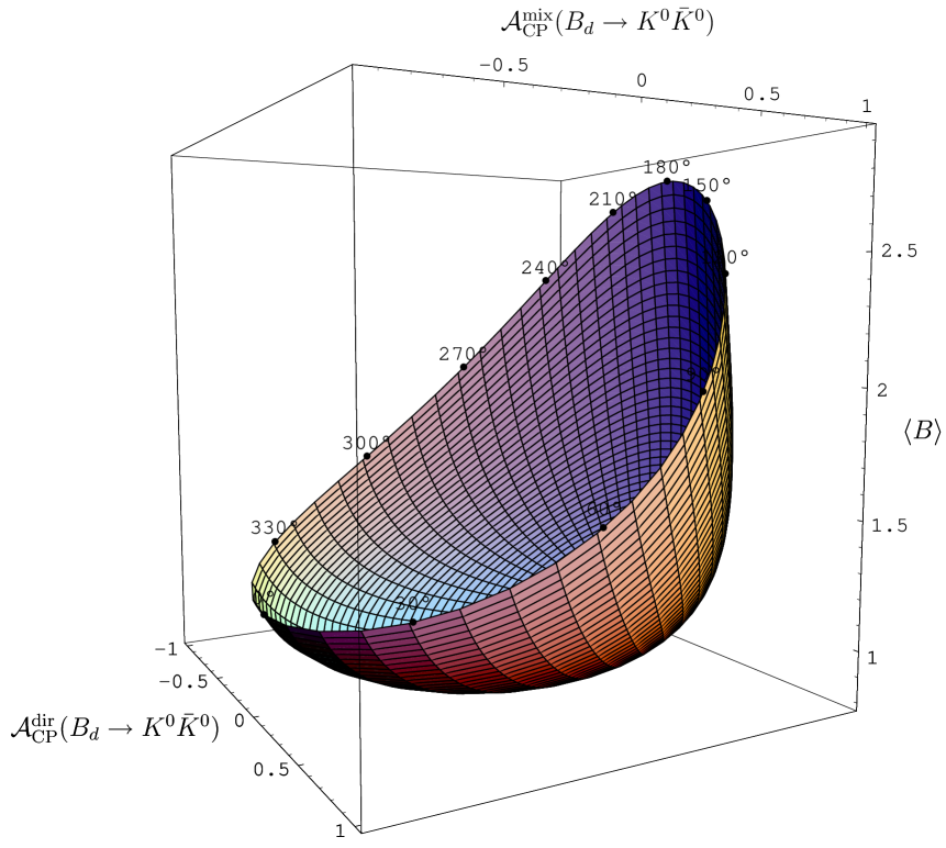
Figure 1: The surface in the ${\cal A}_{\rm CP}^{\rm dir}$–${\cal A}_{\rm CP}^{\rm mix}$–$\langle B\rangle$ observable space of $B^{0}_{d}\to K^{0}\bar{K}^{0}$ for $\phi_{d}=47^{\circ}$ and $\gamma=65^{\circ}$, characterizing this decay in the SM. The intersecting lines on the surface correspond to constant $\rho_{K\!K}$ and $\theta_{K\!K}$, respectively. The numbers on the fringe indicate the value of $\theta_{K\!K}$, the fringe itself is defined by $\rho_{K\!K}=1$.

2.2 Characteristic Surface in Observable Space

In the following analysis, we assume that

$$\phi_{d}=2\beta=(47\pm 4)^{\circ},\quad\gamma=(65\pm 7)^{\circ},$$ (13)

as in the SM [7]. By the time the CP-violating asymmetries in (8) and (9) can be reliably measured, the picture of these parameters will be much sharper. The measurement of ${\cal A}_{\rm CP}^{\rm dir}$ and ${\cal A}_{\rm CP}^{\rm mix}$ allows us then to extract the hadronic parameters $\rho_{K\!K}$ and $\theta_{K\!K}$ in a theoretically clean manner. Although these quantities are interesting for the analysis of charged $B\to\pi K$ modes, as we will see below, and can nicely be compared with theoretical predictions, such as those of the “QCD factorization” approach [8], they do not provide – by themselves – a test of the SM description of the $\bar{b}\to\bar{d}s\bar{s}$ FCNC processes mediating the decay $B^{0}_{d}\to K^{0}\bar{K}^{0}$. However, so far, we have not yet used the information offered by the CP-averaged branching ratio introduced in (1). The parametrization in (5) allows us to write

$$\mbox{BR}(B_{d}\to K^{0}\bar{K}^{0})=\frac{\tau_{B_{d}}}{16\pi M_{B_{d}}}\Phi(M_{K}/M_{B_{d}},M_{K}/M_{B_{d}})|\lambda^{3}A{\cal P}_{tc}^{K\!K}|^{2}\langle B\rangle,$$ (14)

where

$$\Phi(x,y)=\sqrt{\left[1-(x+y)^{2}\right]\left[1-(x-y)^{2}\right]}$$ (15)

is the two-body phase-space function, and

$$\langle B\rangle\equiv 1-2\rho_{K\!K}\cos\theta_{K\!K}\cos\gamma+\rho_{K\!K}^{2}.$$ (16)

If we now use the SM values of $\phi_{d}$ and $\gamma$, we may characterize the decay $B^{0}_{d}\to K^{0}\bar{K}^{0}$ – within the SM – through a surface in the observable space of ${\cal A}_{\rm CP}^{\rm dir}$, ${\cal A}_{\rm CP}^{\rm mix}$ and $\langle B\rangle$. In Fig. 1, we show this surface, where each point corresponds to a given value of $\rho_{K\!K}$ and $\theta_{K\!K}$. It should be emphasized that this surface is theoretically clean since it relies only on the general SM parametrization of $B^{0}_{d}\to K^{0}\bar{K}^{0}$. Consequently, should future measurements give a value in observable space that should not lie on the SM surface, we would have immediate evidence for NP contributions to $\bar{b}\to\bar{d}s\bar{s}$ FCNC processes. If we consider a fixed value of $\langle B\rangle$, we obtain ellipses in the ${\cal A}_{\rm CP}^{\rm dir}$–${\cal A}_{\rm CP}^{\rm mix}$ plane, which are described by

$$\left[\frac{{\cal A}_{\rm CP}^{\rm dir}}{a_{{\cal A}_{\rm CP}^{\rm dir}}}\right]^{2}+\left[\frac{{\cal A}_{\rm CP}^{\rm mix}-{\cal A}_{0}}{a_{{\cal A}_{\rm CP}^{\rm mix}}}\right]^{2}=1,$$ (17)

with

$${\cal A}_{0}=\left[\frac{\langle B\rangle-2\sin^{2}\gamma}{\langle B\rangle}\right]\sin(\phi_{d}+2\gamma)$$ (18)

and

$$a_{{\cal A}_{\rm CP}^{\rm dir}}=2\frac{\sqrt{\langle B\rangle-\sin^{2}\gamma}}{\langle B\rangle}|\sin\gamma|,\quad a_{{\cal A}_{\rm CP}^{\rm mix}}=a_{{\cal A}_{\rm CP}^{\rm dir}}|\cos(\phi_{d}+2\gamma)|.$$ (19)

In Fig. 2, we show these ellipses for various values of $\langle B\rangle$. Since $\sin(\phi_{d}+2\gamma)=0.05$ and $\cos(\phi_{d}+2\gamma)=-1.00$ for the central values of (13), we have actually to deal – to a good approximation – with circles around the origin in the case of this figure.

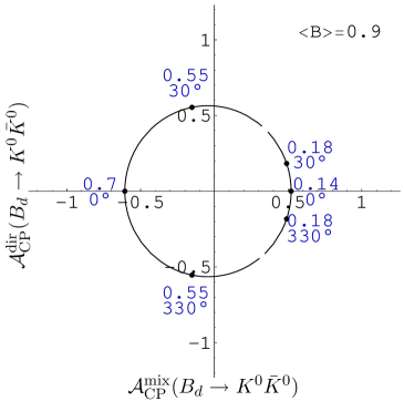
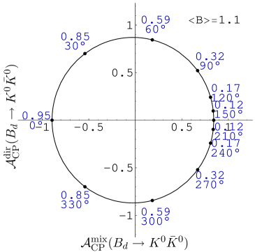
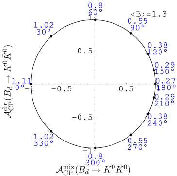
Figure 2: The ellipses arising in the ${\cal A}_{\rm CP}^{\rm mix}$–${\cal A}_{\rm CP}^{\rm dir}$ plane for given values of $\langle B\rangle$, with the associated values of $\rho_{K\!K}$ and $\theta_{K\!K}$. As in Fig. 1, we have chosen $\phi_{d}=47^{\circ}$ and $\gamma=65^{\circ}$.

In the derivation of (17), we have assumed that $\langle B\rangle-\sin^{2}\gamma>0$, which enters in (19). In fact, if we consider (16) and vary $\rho_{K\!K}$ and $\theta_{K\!K}$ as free parameters, while keeping $\gamma$ fixed, we find that $\langle B\rangle$ takes the following absolute minimum:

$$\langle B\rangle_{\rm min}=\sin^{2}\gamma=0.82\,^{+0.08}_{-0.10},$$ (20)

which corresponds to

$$\rho_{K\!K}=\cos\gamma=0.42\pm 0.11,\quad\theta_{K\!K}=0^{\circ},$$ (21)

yielding

$${\cal A}_{\rm CP}^{\rm dir}=0,\quad{\cal A}_{\rm CP}^{\rm mix}=-\sin(\phi_{d}+2\gamma)=-\left(0.05\pm 0.25\right).$$ (22)

The numerical results in (20)–(22) were calculated with the help of (13). It is amusing to note that the associated values of $\rho_{K\!K}$ and $\theta_{K\!K}$ are very close to the case of top-quark dominance, as can be seen in (10).

2.3 Extraction of $\langle B\rangle$

Whereas ${\cal A}_{\rm CP}^{\rm dir}$ and ${\cal A}_{\rm CP}^{\rm mix}$ can be directly obtained from (2), the extraction of $\langle B\rangle$ from (14) requires additional information. To this end, we follow [9], and combine $B_{d}\to K^{0}\bar{K}^{0}$ with $B_{d}\to\pi^{+}\pi^{-}$. It is then useful to write the decay amplitude of the latter mode as

$$A(B^{0}_{d}\to\pi^{+}\pi^{-})=-\lambda^{3}A{\cal P}_{tc}^{\pi\pi}\left[1-e^{i\gamma}\frac{1}{de^{i\theta}}\right],$$ (23)

where ${\cal P}_{tc}^{\pi\pi}$ is the $B_{d}\to\pi^{+}\pi^{-}$ counterpart of ${\cal P}_{tc}^{K\!K}$, and $de^{i\theta}$ is a hadronic parameter. Performing an isospin analysis of the $B\to\pi\pi$ system for the SM values of $\phi_{d}$ and $\gamma$ in (13), $d$ and $\theta$ could be extracted from the $B$-factory data, with the following result [10]:

$$d=0.48\,^{+0.35}_{-0.22},\quad\theta=+\left(138\,^{+19}_{-23}\right)^{\circ};$$ (24)

similar values were subsequently obtained in [11]. If we calculate now the CP-averaged $B_{d}\to\pi^{+}\pi^{-}$ branching ratio with the help of (23), (14) implies

$$\langle B\rangle=\left|\frac{{\cal P}_{tc}^{\pi\pi}}{{\cal P}_{tc}^{K\!K}}\right|^{2}\left[\frac{\mbox{BR}(B_{d}\to K^{0}\bar{K}^{0})}{\mbox{BR}(B_{d}\to\pi^{+}\pi^{-})}\right]F_{\pi\pi}(d,\theta),$$ (25)

where we have introduced

$$F_{\pi\pi}(d,\theta)\equiv\frac{1-2d\cos\theta\cos\gamma+d^{2}}{d^{2}}=6.57\,^{+6.65}_{-4.20},$$ (26)

and have neglected tiny phase-space differences. The numerical value in (26) follows from the $B\to\pi\pi$ analysis performed in [10]. In the future, the corresponding uncertainties, which are only of experimental origin, can be reduced considerably. Let us emphasize that (25) is valid exactly in the SM. In order to deal with the $|{\cal P}_{tc}^{\pi\pi}/{\cal P}_{tc}^{K\!K}|$ factor, we neglect colour-suppressed EW penguins, which have an essentially negligible impact on the $B_{d}\to K^{0}\bar{K}^{0}$ and $B_{d}\to\pi^{+}\pi^{-}$ modes [12], and use the $SU(3)$ flavour symmetry of strong interactions. In the strict $SU(3)$ limit, this ratio equals one. If we take the factorizable $SU(3)$-breaking corrections into account, we obtain

$$\left|\frac{{\cal P}_{tc}^{\pi\pi}}{{\cal P}_{tc}^{K\!K}}\right|_{\rm fact}=\left[\frac{f_{\pi}F_{B\pi}(M_{\pi}^{2};0^{+})}{f_{K}F_{BK}(M_{K}^{2};0^{+})}\right]\left[\frac{M_{B}^{2}-M_{\pi}^{2}}{M_{B}^{2}-M_{K}^{2}}\right]=0.64,$$ (27)

where $f_{\pi}=131\,{\rm MeV}$ and $f_{K}=160\,{\rm MeV}$ denote the pion and kaon decay constants, and the form factors $F_{B\pi}(M_{\pi}^{2};0^{+})$ and $F_{BK}(M_{K}^{2};0^{+})$ parametrize the hadronic quark-current matrix elements $\langle\pi^{-}|(\bar{b}u)_{\rm V-A}|B^{0}_{d}\rangle$ and $\langle K^{0}|(\bar{b}s)_{\rm V-A}|B^{0}_{d}\rangle$, respectively. The numerical value in (27) corresponds to the light-cone sum-rule analysis performed recently in [14] (with $\delta_{a1}=0$), while the form factors obtained within the Bauer–Stech–Wirbel (BSW) model [15] yield a value of 0.72.

2.4 Exploring Non-Factorizable $SU(3)$-Breaking Corrections

Insights into the issue of factorization and $SU(3)$-breaking effects of the hadronic ${\cal P}_{tc}$ penguin amplitudes can be obtained with the help of $B\to\pi K$ modes, which originate from $\bar{b}\to\bar{s}$ quark-level processes. Applying the formalism of [10], we write

$$\left[\frac{\mbox{BR}(B^{\pm}\to\pi^{\pm}K)}{\mbox{BR}(B_{d}\to\pi^{+}\pi^{-})}\right]\left[\frac{\tau_{B_{d}}}{\tau_{B^{+}}}\right]=\frac{1}{\epsilon}\left|\frac{{\cal P}_{tc}^{\pi K}}{{\cal P}_{tc}^{\pi\pi}}\right|^{2}\left[\frac{1+\delta R}{F_{\pi\pi}(d,\theta)}\right],$$ (28)

where

$$\epsilon\equiv\frac{\lambda^{2}}{1-\lambda^{2}}=0.05,$$ (29)

and

$$\delta R=2\rho_{\rm c}\cos\theta_{\rm c}\cos\gamma+\rho_{\rm c}^{2}-2\left[\cos\psi_{\rm C}^{(1)}+\rho_{\rm c}\cos(\theta_{\rm c}-\psi_{\rm C}^{(1)})\cos\gamma\right]a_{\rm EW}^{{\rm C}(1)}+\left[a_{\rm EW}^{{\rm C}(1)}\right]^{2}.$$ (30)

The hadronic parameter $\rho_{\rm c}e^{i\theta_{\rm c}}$ is the $B^{+}\to\pi^{+}K^{0}$ counterpart of $\rho_{K\!K}e^{i\theta_{K\!K}}$. Because of the different CKM structure of $B^{+}\to\pi^{+}K^{0}$, we have

$$\rho_{\rm c}e^{i\theta_{\rm c}}\approx\epsilon\,\rho_{K\!K}e^{i\theta_{K\!K}},$$ (31)

so that $\rho_{\rm c}$ is expected at the few percent level. The parameter $a_{\rm EW}^{{\rm C}(1)}$ and the strong phase $\psi_{\rm C}^{(1)}$ are related to colour-suppressed EW penguins. It is expected that $a_{\rm EW}^{{\rm C}(1)}$ is also of ${\cal O}(10^{-2})$. Interestingly, the analysis performed in [10] allows us to determine $\delta R$ from the data with the help of the following relation:

$$1+\delta R=\frac{1-2r\cos\delta\cos\gamma+r^{2}}{R},$$ (32)

where

$$R\equiv\left[\frac{\mbox{BR}(B_{d}^{0}\to\pi^{-}K^{+})+\mbox{BR}(\bar{B}_{d}^{0}\to\pi^{+}K^{-})}{\mbox{BR}(B^{+}\to\pi^{+}K^{0})+\mbox{BR}(B^{-}\to\pi^{-}\bar{K}^{0})}\right]\frac{\tau_{B^{+}}}{\tau_{B_{d}}}=0.91\pm 0.07,$$ (33)

and the hadronic parameters

$$r=0.11^{+0.07}_{-0.05},\quad\delta=+(42^{+23}_{-19})^{\circ}$$ (34)

were fixed through

$$re^{i\delta}=\frac{\epsilon}{d}e^{i(\pi-\theta)}$$ (35)

from the $B\to\pi\pi$ analysis, which yields (24). Following these lines, we obtain

$$\delta R=0.036\,^{+0.094}_{-0.079},$$ (36)

which is nicely complemented by the experimental results [5] for the direct CP asymmetry

$${\cal A}_{\rm CP}^{\rm dir}(B^{\pm}\to\pi^{\pm}K)\equiv\frac{\mbox{BR}(B^{+}\to\pi^{+}K^{0})-\mbox{BR}(B^{-}\to\pi^{-}\bar{K}^{0})}{\mbox{BR}(B^{+}\to\pi^{+}K^{0})+\mbox{BR}(B^{-}\to\pi^{-}\bar{K}^{0})}=-0.02\pm 0.06,$$ (37)

taking the following form:

$${\cal A}_{\rm CP}^{\rm dir}(B^{\pm}\to\pi^{\pm}K)=-2\rho_{\rm c}\left[\frac{\sin\theta_{\rm c}-a_{\rm EW}^{{\rm C}(1)}\sin(\theta_{\rm c}-\psi_{\rm C}^{(1)})}{1+\delta R}\right]\sin\gamma.$$ (38)

Consequently, we have no experimental evidence for anomalously large values of $\rho_{\rm c}$ and $a_{\rm EW}^{{\rm C}(1)}$. In particular, we do not find indications for an enhancement of the latter parameter describing the colour-suppressed EW penguin contributions, in contrast to the claims made recently in [16].

If we write now

$$\left|\frac{{\cal P}_{tc}^{\pi\pi}}{{\cal P}_{tc}^{\pi K}}\right|=\xi_{SU(3)}^{\rm n-fact}\left|\frac{{\cal P}_{tc}^{\pi\pi}}{{\cal P}_{tc}^{\pi K}}\right|_{\rm fact}\quad\mbox{with}\quad\left|\frac{{\cal P}_{tc}^{\pi\pi}}{{\cal P}_{tc}^{\pi K}}\right|_{\rm fact}=\frac{f_{\pi}}{f_{K}},$$ (39)

we obtain from (28) with the help of (32) and (35)

$$\xi_{SU(3)}^{\rm n-fact}=\frac{f_{K}}{f_{\pi}}\sqrt{\frac{1}{\epsilon}\left[\frac{d^{2}+2\epsilon d\cos\theta\cos\gamma+\epsilon^{2}}{1-2d\cos\theta\cos\gamma+d^{2}}\right]\left[\frac{\mbox{BR}(B_{d}\to\pi^{+}\pi^{-})}{\mbox{BR}(B_{d}\to\pi^{\mp}K^{\pm})}\right]}=1.01^{+0.48}_{-0.37},$$ (40)

where the numerical value follows from the analysis in [10]. The current $B$-factory data do therefore not indicate a deviation of $\xi_{SU(3)}^{\rm n-fact}$ from one, although the uncertainties are still large. In the future, (40) can be determined with much better accuracy. In particular, since this expression involves only $B$ decays with charged pions and kaons in the final state, it should be possible to explore it in a powerful way at LHCb [17]. A similar comment applies to the determination of (26). It should be noted that (40) does actually not only probe non-factorizable $SU(3)$-breaking effects, but also the importance of penguin annihilation topologies, which contribute to $B_{d}\to\pi^{+}\pi^{-}$ and $B_{d}\to K^{0}\bar{K}^{0}$ (and are implicitly included in ${\cal P}_{tc}^{\pi\pi}$ and ${\cal P}_{tc}^{K\!K}$, respectively), but do not contribute to ${\cal P}_{tc}^{\pi K}$. Their importance can be explored through the $B_{d}\to K^{+}K^{-}$, $B_{s}\to\pi^{+}\pi^{-}$ system. The experimental upper bounds on the former decay [10], as well as the numerical value in (40), do not indicate any enhancement.

2.5 Lower Bounds on the $B_{d}\to K^{0}\bar{K}^{0}$ Branching Ratio

By the time all $B_{d}\to K^{0}\bar{K}^{0}$ observables can be measured with a reasonable accuracy, we will have a good picture of (40). We may then extrapolate correspondingly to the determination of $|{\cal P}_{tc}^{\pi\pi}/{\cal P}_{tc}^{K\!K}|$ through (27), allowing us to relate $\langle B\rangle$ to the CP-averaged $B_{d}\to K^{0}\bar{K}^{0}$ branching ratio with the help of (25). For the following analysis, we will just use (27), complementing it with the numerical result in (26) and $\mbox{BR}(B_{d}\to\pi^{+}\pi^{-})=(4.6\pm 0.4)\times 10^{-6}$ [5]. We are then in a position to convert the lower bound in (20) into the following lower bound for the CP-averaged $B_{d}\to K^{0}\bar{K}^{0}$ branching ratio:

$$\mbox{BR}(B_{d}\to K^{0}\bar{K}^{0})_{\rm min}=\left(1.39^{+1.54}_{-0.95}\right)\times\left[\frac{F_{BK}(M_{K}^{2};0^{+})}{0.331}\frac{0.258}{F_{B\pi}(M_{\pi}^{2};0^{+})}\right]^{2}\times 10^{-6}.$$ (41)

In this expression, we made the dependence on the form factors explicit, where the numerical values refer to [14]. If we use the BSW form factors [15], the lower bound on $\mbox{BR}(B_{d}\to K^{0}\bar{K}^{0})$ is reduced by about $20\%$.

Interestingly, a picture similar to the one of (41) emerges also from a very different avenue: it is a nice feature of (25) that this relation uses only $\bar{b}\to\bar{d}$ transitions. However, it is also useful to combine $B^{0}_{d}\to K^{0}\bar{K}^{0}$ with the $\bar{b}\to\bar{s}$ transition $B^{+}\to\pi^{+}K^{0}$. As we have noted above, in doing this we have to neglect the penguin annihilation topologies contributing to the former mode. Neglecting phase-space differences for simplicity, we may then write

$$\langle B\rangle=\frac{1}{\epsilon}\left|\frac{{\cal P}_{tc}^{\pi K}}{{\cal P}_{tc}^{K\!K}}\right|^{2}(1+\delta R)\left[\frac{\mbox{BR}(B_{d}\to K^{0}\bar{K}^{0})}{\mbox{BR}(B^{\pm}\to\pi^{\pm}K)}\right]\frac{\tau_{B^{+}}}{\tau_{B_{d}}},$$ (42)

where

$$\left|\frac{{\cal P}_{tc}^{\pi K}}{{\cal P}_{tc}^{K\!K}}\right|_{\rm fact}=\left[\frac{F_{B\pi}(M_{K}^{2};0^{+})}{F_{BK}(M_{K}^{2};0^{+})}\right]\left[\frac{M_{B}^{2}-M_{\pi}^{2}}{M_{B}^{2}-M_{K}^{2}}\right]=0.79.$$ (43)

The numerical value in (43) corresponds again to the light-cone sum-rule analysis performed in [14] (with $\delta_{a1}=0$). If we now use $\mbox{BR}(B^{\pm}\to\pi^{\pm}K)=(21.8\pm 1.4)\times 10^{-6}$ [5], $\tau_{B^{+}}/\tau_{B_{d}}=1.086\pm 0.017$, as well as (36) and (43), (42) allows us to convert (20) into the following lower bound:

$$\mbox{BR}(B_{d}\to K^{0}\bar{K}^{0})_{\rm min}=\left(1.36^{+0.18}_{-0.21}\right)\times\left[\frac{F_{BK}(M_{K}^{2};0^{+})}{0.331}\frac{0.258}{F_{B\pi}(M_{K}^{2};0^{+})}\right]^{2}\times 10^{-6}.$$ (44)

In comparison with (25), the advantage of (42) is obviously that the $B\to\pi\pi$ analysis enters only through $\delta R$, which has a small numerical impact. This feature is nicely reflected by the errors of (44), which are considerably reduced with respect of (41), while the central values are very similar. On the other hand, we have to rely on the neglect of the penguin annihilation topologies in $B^{0}_{d}\to K^{0}\bar{K}^{0}$, so that (25) is conceptually more favourable.

In view of the different assumptions entering (41) and (44), we consider it as very remarkable to arrive at such a consistent picture (see also (40)). Looking at (1), we observe that these lower SM bounds are very close to the current experimental upper bound, thereby suggesting that the observation of the decay $B_{d}^{0}\to K^{0}\bar{K}^{0}$ at the $B$ factories is just ahead of us. If we assume again that the penguin annihilation contributions to $B^{0}_{d}\to K^{0}\bar{K}^{0}$ are small, the decay $B^{+}\to K^{+}\bar{K}^{0}$ has a very similar branching ratio; the current experimental upper bound is given by $2.5\times 10^{-6}$ ($90\%$ C.L.) [5]. The latter mode is the $U$-spin counterpart of $B^{+}\to\pi^{+}K^{0}$, i.e. both channels are related to each other by interchanging all down and strange quarks, and was discussed in the context of dealing with the parameter $\rho_{\rm c}$ [10, 18].

2.6 Upper Bounds on $\langle B\rangle$ and $\rho_{K\!K}$

It is also interesting to convert the experimental upper bound in (1) into upper bounds for $\langle B\rangle$. Using (25) and (42), we obtain

$$\langle B\rangle_{\rm max}=\left(0.88^{+0.90}_{-0.57}\right)\times\left[\frac{F_{B\pi}(M_{\pi}^{2};0^{+})}{0.258}\frac{0.331}{F_{BK}(M_{K}^{2};0^{+})}\right]^{2}\times\left[{\mbox{BR}(B_{d}\to K^{0}\bar{K}^{0})\over 1.5\times 10^{-6}}\right]$$ (45)

and

$$\langle B\rangle_{\rm max}=\left(0.91^{+0.10}_{-0.09}\right)\times\left[\frac{F_{B\pi}(M_{K}^{2};0^{+})}{0.258}\frac{0.331}{F_{BK}(M_{K}^{2};0^{+})}\right]^{2}\times\left[{\mbox{BR}(B_{d}\to K^{0}\bar{K}^{0})\over 1.5\times 10^{-6}}\right],$$ (46)

respectively. We observe that the numerical values in (45) and (46) are very close to the lower bound in (20), which is of course no surprise because of the discussion given above. The interesting aspect of an upper bound for $\langle B\rangle$ is that it allows us to obtain an upper bound for $\rho_{K\!K}$ with the help of the following relation:

$$\rho_{K\!K}<\left|\cos\gamma\right|+\sqrt{\langle B\rangle_{\rm max}-\sin^{2}\gamma},$$ (47)

where the central values in (45) and (46) correspond for $\gamma=65^{\circ}$ to $\rho_{K\!K}<0.66$ and $\rho_{K\!K}<0.72$, respectively, but the uncertainties remain sizeable.

Looking at (31), we see that these upper bounds for $\rho_{K\!K}$ imply that $\rho_{\rm c}$ is actually tiny, in accordance with the discussion after (38). In [10], the experimental upper bound for BR$(B^{\pm}\to K^{\pm}K)$ discussed above was converted into $\rho_{\rm c}<0.1$ with the help of the $U$-spin relation to BR$(B^{\pm}\to\pi^{\pm}K)$, which would conversely correspond to $\rho_{K\!K}\mathrel{\hbox{\hbox to0.0pt{\hbox{\lower 4.0pt\hbox{$\sim$}}\hss}\hbox{$<$}}}2$. Consequently, (47) yields stronger constraints on this parameter.

2.7 Comments on a Different Avenue: Extraction of $\gamma$

The analysis discussed above depends on the value of $\gamma$. This parameter enters explicitly in the corresponding formulae, but also implicitly through the values of $d$ and $\theta$ in (24), which follow from the direct and mixing-induced CP asymmetries of $B_{d}\to\pi^{+}\pi^{-}$ and are actually functions of $\gamma$ [10]. However, if we do not assume that $\gamma$ is known, it is easy to see that the determination of the three $B_{d}\to K^{0}\bar{K}^{0}$ observables ${\cal A}_{\rm CP}^{\rm dir}$, ${\cal A}_{\rm CP}^{\rm mix}$ and $\langle B\rangle$ allows us to extract simultaneously $\rho_{K\!K}$, $\theta_{K\!K}$ and $\gamma$, up to discrete ambiguities. This feature is not surprising, since it was suggested in [9] to complement the CP-violating $B_{d}\to\pi^{+}\pi^{-}$ asymmetries with the observables provided by $B_{d}\to K^{0}\bar{K}^{0}$ to deal with the famous penguin problem in the former channel and to determine the angle $\alpha$ of the unitarity triangle. We have just encountered a different implementation of this strategy. Alternative methods to extract $\gamma$ from $B_{d}\to K^{0}\bar{K}^{0}$ were proposed in [19], combining this channel with its $U$-spin partner $B_{s}\to K^{0}\bar{K}^{0}$.

3 Correlations with the $B\to\pi\pi$ System

The decay $B^{0}_{d}\to K^{0}\bar{K}^{0}$ will also allow us to obtain valuable insights into the substructure of the $B\to\pi\pi$ system. In the analysis of these decays in [10], another hadronic parameter,

$$xe^{i\Delta}\equiv\frac{{\cal C}_{\pi\pi}+({\cal P}_{tu}^{\pi\pi}-{\cal E}_{\pi\pi})}{{\cal T}_{\pi\pi}-({\cal P}_{tu}^{\pi\pi}-{\cal E}_{\pi\pi})},$$ (48)

was introduced, where ${\cal C}_{\pi\pi}$ and ${\cal T}_{\pi\pi}$ are the strong amplitudes of colour-suppressed and colour-allowed tree-diagram-like topologies, respectively, ${\cal P}_{tu}^{\pi\pi}\equiv{\cal P}_{t}^{\pi\pi}-{\cal P}_{u}^{\pi\pi}$ is defined in analogy to ${\cal P}_{tc}^{\pi\pi}$, and ${\cal E}_{\pi\pi}$ describes an exchange topology. In analogy to the determination of $d$ and $\theta$ (see (24)), $x$ and $\Delta$ can also be extracted from the $B\to\pi\pi$ data, with the following result:

$$x=1.22^{+0.26}_{-0.21},\quad\Delta=-\left(71^{+19}_{-26}\right)^{\circ}.$$ (49)

If we now introduce the “colour-suppression” parameter

$$a_{2}^{\pi\pi}e^{i\Delta_{2}^{\pi\pi}}\equiv\frac{{\cal C}_{\pi\pi}}{{\cal T}_{\pi\pi}},$$ (50)

neglect the exchange amplitude ${\cal E}_{\pi\pi}$, which is expected to play a minor rôle and can be explored with the help of the $B_{d}\to K^{+}K^{-}$, $B_{s}\to\pi^{+}\pi^{-}$ system [10], and use the $SU(3)$ flavour symmetry of strong interactions, we obtain

$$\rho_{K\!K}e^{i\theta_{K\!K}}=\left[\frac{a_{2}^{\pi\pi}e^{i\Delta_{2}^{\pi\pi}}-xe^{i\Delta}}{a_{2}^{\pi\pi}e^{i\Delta_{2}^{\pi\pi}}+1}\right]\frac{e^{-i\theta}}{d}.$$ (51)

In Fig. 3, we illustrate the resulting contours in the $\theta_{K\!K}$–$\rho_{K\!K}$ plane for various values of $a_{2}^{\pi\pi}$ and $\Delta_{2}^{\pi\pi}\in[0^{\circ},360^{\circ}]$, taking also into account that values of $\rho_{K\!K}$ being significantly larger than 1 are disfavoured because of the discussion in Subsection 2.6. In order to simplify the analysis, we have considered the central values of $(d,\theta)$ and $(x,\Delta)$ in (24) and (49), respectively. By the time the CP-violating $B_{d}\to K^{0}\bar{K}^{0}$ observables can be measured, much more accurate determinations of these parameters will anyway be available. As soon as $\rho_{K\!K}$ and $\theta_{K\!K}$ are extracted from the $B_{d}\to K^{0}\bar{K}^{0}$ observables, (51) allows us to determine $a_{2}^{\pi\pi}$ and $\Delta_{2}^{\pi\pi}$ with the help of

$$a_{2}^{\pi\pi}e^{i\Delta_{2}^{\pi\pi}}=\frac{xe^{i\Delta}+de^{i\theta}\rho_{K\!K}e^{i\theta_{K\!K}}}{1-de^{i\theta}\rho_{K\!K}e^{i\theta_{K\!K}}}.$$ (52)

Following [10], we may then also determine the hadronic parameter $\zeta_{\pi\pi}e^{i\Delta_{\zeta}^{\pi\pi}}\equiv{\cal P}_{tu}^{\pi\pi}/{\cal T}_{\pi\pi}$, as well as ${\cal P}_{tc}^{\pi\pi}/{\cal T}_{\pi\pi}$, so that we are in a position to resolve the whole substructure of the $B\to\pi\pi$ system. In particular, we may then pin down the interference effects between the different hadronic penguin amplitudes, and may decide which one of the patterns suggested in the literature (see, for instance, [10, 20]) is actually realized in nature.

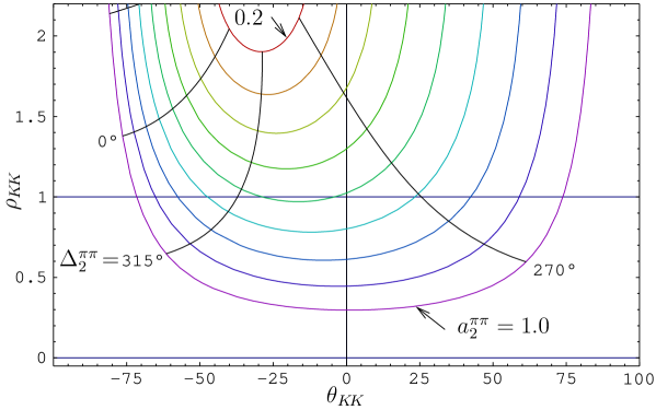
Figure 3: The contours in the $\theta_{K\!K}$–$\rho_{K\!K}$ plane corresponding to the central values of $(d,\theta)$ and $(x,\Delta)$ in (24) and (49), respectively, for various values of $a_{2}^{\pi\pi}$ and $\Delta_{2}^{\pi\pi}\in[0^{\circ},360^{\circ}]$.

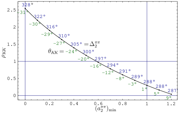
Figure 4: The correlation between the upper bound for $\rho_{K\!K}$ and the corresponding lower bound for $a_{2}^{\pi\pi}$ with the associated values of $\theta_{K\!K}$ and $\Delta_{2}^{\pi\pi}$ for the case shown in Fig. 3.

If we look at Fig. 3, we observe that upper bounds for $\rho_{K\!K}$ correspond to lower bounds for $a_{2}^{\pi\pi}$, as illustrated in Fig. 4. For $\rho_{K\!K}\mathrel{\hbox{\hbox to0.0pt{\hbox{\lower 4.0pt\hbox{$\sim$}}\hss}\hbox{$<$}}}0.9$, we obtain $a_{2}^{\pi\pi}\mathrel{\hbox{\hbox to0.0pt{\hbox{\lower 4.0pt\hbox{$\sim$}}\hss}\hbox{$>$}}}0.6$. Consequently, the rather stringent upper bounds for $\rho_{K\!K}$ following from (47) require a sizeable deviation from the naïve value of $a_{2}^{\pi\pi}e^{i\Delta_{2}^{\pi\pi}}\sim 0.25$. This observation is in accordance with discussion given in [10], putting it on more solid ground. In this picture, we have destructive interference between the ${\cal P}_{t}^{\pi\pi}$ and ${\cal P}_{c}^{\pi\pi}$ amplitudes, whereas the interference between ${\cal P}_{t}^{\pi\pi}$ and ${\cal P}_{u}^{\pi\pi}$ is constructive, with $|{\cal P}_{t}^{\pi\pi}/{\cal T}_{\pi\pi}|\sim|{\cal P}_{u}^{\pi\pi}/{\cal T}_{\pi\pi}|\sim 0.25$. Moreover, $0.5\mathrel{\hbox{\hbox to0.0pt{\hbox{\lower 4.0pt\hbox{$\sim$}}\hss}\hbox{$<$}}}a_{2}^{\pi\pi}\mathrel{\hbox{\hbox to0.0pt{\hbox{\lower 4.0pt\hbox{$\sim$}}\hss}\hbox{$<$}}}0.7$ with $\Delta_{2}^{\pi\pi}\sim 290^{\circ}$ is suggested, where $\rho_{K\!K}$ is actually close to its current experimental upper bounds discussed in Subsection 2.6, as can be seen in Fig. 4.

Let us finally come back to the CP-violating observables ${\cal A}_{\rm CP}^{\rm dir}$ and ${\cal A}_{\rm CP}^{\rm mix}$ of the decay $B^{0}_{d}\to K^{0}\bar{K}^{0}$. In Fig. 5, we consider the ${\cal A}_{\rm CP}^{\rm mix}$–${\cal A}_{\rm CP}^{\rm dir}$ plane and show the contours for different values of $a_{2}^{\pi\pi}$, where each point is parametrized by a given value of $\Delta_{2}^{\pi\pi}$. In accordance with our upper bounds for $\rho_{K\!K}$, we assume that $\rho_{K\!K}<0.9$; the contours are dashed where this bound is violated. The shaded region is calculated with the help of (51) for the central values of $(d,\theta)$ and $(x,\Delta)$ in (24) and (49), respectively, imposing the constraints of $\rho_{K\!K}<0.9$ and $a_{2}^{\pi\pi}<0.9$. As far as the latter bound is concerned, we allow for values being significantly larger than the range discussed above to be on the conservative side. From the position of the contours it can be seen how this region changes for different upper bounds on $a_{2}^{\pi\pi}$. We observe that an interesting pattern emerges, where negative values of the mixing-induced $B^{0}_{d}\to K^{0}\bar{K}^{0}$ CP asymmetry are preferred. In order to complement Fig. 5, we show in Fig. 6 the curve corresponding to the correlation between the lower bounds on $a_{2}^{\pi\pi}$ that are implied by upper bounds on $\rho_{K\!K}$, as illustrated in Fig. 4.

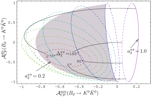
Figure 5: The contours in the ${\cal A}_{\rm CP}^{\rm mix}$–${\cal A}_{\rm CP}^{\rm dir}$ plane corresponding to different values of $a_{2}^{\pi\pi}$ between 0.2 and 1. The contours are drawn solid for $\rho_{K\!K}\leq 0.9$ and dashed for $\rho_{K\!K}>0.9$. The shaded region illustrates the area where $a_{2}^{\pi\pi}<0.9$ and $\rho_{K\!K}<0.9$.

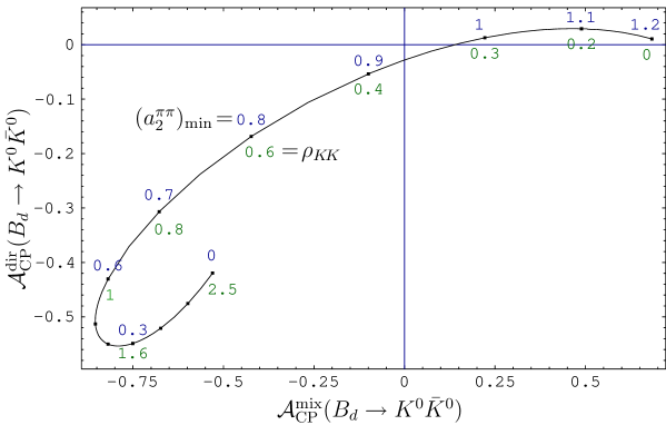
Figure 6: The contour in the ${\cal A}_{\rm CP}^{\rm mix}$–${\cal A}_{\rm CP}^{\rm dir}$ plane arising for the limiting case illustrated in Fig. 4. The numbers below and above the curve correspond to the given upper bound for $\rho_{K\!K}$ and the associated minimal value of $a_{2}^{\pi\pi}$, respectively.

It should be noted that the analysis performed in this section – and the pattern in the ${\cal A}_{\rm CP}^{\rm mix}$–${\cal A}_{\rm CP}^{\rm dir}$ plane – do not depend on the $SU(3)$-breaking ratio of the $F_{B\pi}$ and $F_{BK}$ form factors that we encountered in Section 2. This quantity enters only implicitly when we impose the upper bounds for $\rho_{K\!K}$ that are extracted from the current $B$-factory data.

4 Conclusions

In our analysis of the penguin mode $B^{0}_{d}\to K^{0}\bar{K}^{0}$, we have first shown that this channel can be efficiently characterized in the SM through a theoretically clean surface in the space of its observables ${\cal A}_{\rm CP}^{\rm dir}$, ${\cal A}_{\rm CP}^{\rm mix}$ and $\langle B\rangle$. Whereas the CP asymmetries can straightforwardly be determined from time-dependent rate measurements, the extraction of $\langle B\rangle$ from the CP-averaged $B^{0}_{d}\to K^{0}\bar{K}^{0}$ branching ratio requires additional information. This can be obtained from the $B\to\pi\pi$ system with the help of the $SU(3)$ flavour symmetry, including the factorizable $SU(3)$-breaking corrections through an appropriate form-factor ratio; we have also discussed how insights into non-factorizable $SU(3)$-breaking corrections of the relevant hadronic penguin amplitudes can be obtained, and have shown that the current $B$-factory data are consistent with small effects, although the errors are still large. Alternatively, $\langle B\rangle$ can also be determined with the help of the CP-averaged $B^{\pm}\to\pi^{\pm}K$ branching ratio, requiring the additional assumption of small penguin annihilation contributions to $B^{0}_{d}\to K^{0}\bar{K}^{0}$. For our numerical analysis, we have used the $SU(3)$-breaking form factor ratio obtained in a recent light-cone sum-rule calculation, which is consistent with the BSW model; further analyses are desirable.

Following these lines, we pointed out that there is a lower bound for the CP-averaged $B_{d}\to K^{0}\bar{K}^{0}$ branching ratio within the SM, where the $B\to\pi\pi$ and $B^{\pm}\to\pi^{\pm}K$ avenues give remarkably consistent pictures. The interesting feature of this lower bound is that it is found to be very close to the current experimental upper bound. Consequently, we expect that the decay $B^{0}_{d}\to K^{0}\bar{K}^{0}$ will soon be observed at the $B$ factories.

Finally, we have explored the interplay between $B^{0}_{d}\to K^{0}\bar{K}^{0}$ and the $B\to\pi\pi$ system, where the former channel allows us to resolve the whole hadronic substructure of the latter modes. In particular, we have shown that upper bounds for $\rho_{K\!K}$ imply lower bounds for the colour-suppression factor $a_{2}^{\pi\pi}$, pointing to a sizeable deviation from the naïve value of $a_{2}^{\pi\pi}e^{i\Delta_{2}^{\pi\pi}}\sim 0.25$. Moreover, we have analysed the impact on the allowed region in the plane of the CP-violating $B_{d}\to K^{0}\bar{K}^{0}$ observables, and found that the current $B$-factory data have a preference for negative values of the corresponding mixing-induced CP asymmetry ${\cal A}_{\rm CP}^{\rm mix}$. By the time these quantities can be measured, we will have a much better picture of the parameters entering this analysis, allowing us to perform an interesting test of the SM description of $\bar{b}\to\bar{d}s\bar{s}$ FCNC processes, which are currently essentially unexplored. The full implementation of these strategies should provide an interesting playground for an $e^{+}e^{-}$ super $B$-factory.

Acknowledgements
The work presented here was supported in part by the German Bundesministerium für Bildung und Forschung under the contract 05HT4WOA/3 and the DFG project Bu. 706/1-2.

References

- [1] M. Kobayashi and T. Maskawa, Prog. Theor. Phys. 49 (1973) 652.
- [2] R. Fleischer, CERN-PH-TH/2004-085 [hep-ph/0405091].
- [3] H.R. Quinn, Nucl. Phys. Proc. Suppl. 37A (1994) 21.
- [4] R. Fleischer, Phys. Lett. B341 (1994) 205.
- [5] Heavy Flavour Averaging Group, http://www.slac.stanford.edu/xorg/hfag/.
-
[6]
L. Wolfenstein,
Phys. Rev. Lett. 51 (1983) 1945;
A.J. Buras, M.E. Lautenbacher and G. Ostermaier, Phys. Rev. D50 (1994) 3433. - [7] M. Battaglia et al., CERN 2003-002-corr [hep-ph/0304132].
- [8] M. Beneke, G. Buchalla, M. Neubert and C.T. Sachrajda, Phys. Rev. Lett. 83 (1999) 1914; M. Beneke and M. Neubert, Nucl. Phys. B675 (2003) 333.
- [9] A.J. Buras and R. Fleischer, Phys. Lett. B360 (1995) 138.
- [10] A.J. Buras, R. Fleischer, S. Recksiegel and F. Schwab, Phys. Rev. Lett. 92 (2004) 101804; CERN-PH-TH/2004-020 [hep-ph/0402112], to appear in Nucl. Phys. B.
-
[11]
A. Ali, E. Lunghi and A.Y. Parkhomenko,
hep-ph/0403275;
C.W. Chiang, M. Gronau, J.L. Rosner and D.A. Suprun, hep-ph/0404073. - [12] M. Gronau, O.F. Hernández, D. London and J.L. Rosner, Phys. Rev. D52 (1995) 6374.
- [13] R. Fleischer, Phys. Lett. B459 (1999) 306.
- [14] P. Ball and R. Zwicky, IPPP-04-23 [hep-ph/0406232].
- [15] M. Bauer, B. Stech and M. Wirbel, Z. Phys. C34 (1987) 103 and C29 (1985) 637.
- [16] J. Charles et al., CPT-2004-P-030 [hep-ph/0406184].
- [17] P. Ball et al., CERN-TH/2000-101 [hep-ph/0003238].
-
[18]
A.J. Buras, R. Fleischer and T. Mannel,
Nucl. Phys. B533 (1998) 3;
A.F. Falk, A.L. Kagan, Y. Nir and A.A. Petrov, Phys. Rev. D57 (1998) 4290. - [19] R. Fleischer, Phys. Rev. D60 (1999) 073008; Phys. Rep. 370 (2002) 537.
- [20] M. Ciuchini, E. Franco, G. Martinelli, M. Pierini and L. Silvestrini, Phys. Lett. B515 (2001) 33; C.W. Bauer, D. Pirjol, I.Z. Rothstein and I.W. Stewart, hep-ph/0401188.