The Gluon Green’s Function at Small x

Abstract

In this contribution a recently proposed iterative procedure is used to study the BFKL gluon Green’s function at next–to–leading order. This is done in QCD and in N=4 supersymmetric Yang–Mills theory. The study includes an analysis of the evolution with energy and of angular dependences. A discussion of a novel resummation of running coupling terms in the QCD case is included.

1 Introduction

The Balitsky–Fadin–Kuraev–Lipatov (BFKL) [1] equation resums a class of logarithms dominant in the Regge limit of scattering amplitudes where the centre of mass energy $\sqrt{s}$ is large and the momentum transfer $\sqrt{-t}$ is fixed. The energy dependence of the cross section is carried by the gluon Green’s function (GGF), which describes the interaction among Reggeised gluons exchanged in the $t$–channel. The GGF carries a dependence on the transverse momenta of the exchanged gluons, $\vec{k}_{a,b}$, and evolves with energy following the BFKL equation, with the rapidity, Y, playing the role of a time variable. The equation can be written in terms of a Mellin transform in Y of the GGF,

$$f\left(\vec{k}_{a},\vec{k}_{b},{\rm Y}\right) = \int_{a-i\infty}^{a+i\infty}\frac{d\omega}{2\pi i}~{}e^{\omega{\rm Y}}f_{\omega}\left(\vec{k}_{a},\vec{k}_{b}\right),$$ (1)

and reads

$$\omega f_{\omega}\left(\vec{k}_{a},\vec{k}_{b}\right) = \delta^{(2)}\left(\vec{k}_{a}-\vec{k}_{b}\right)+\int d^{2}\vec{k}^{\prime}~{}\mathcal{K}\left(\vec{k}_{a},\vec{k}^{\prime}\right)f_{\omega}\left(\vec{k}^{\prime},\vec{k}_{b}\right).$$ (2)

The kernel, $\mathcal{K}$, is known at next–to-leading (NLL) accuracy where terms of the form $\left(\alpha_{s}{\rm Y}\right)^{n}$ and $\alpha_{s}\left(\alpha_{s}{\rm Y}\right)^{n}$ are resummed [2, 3]. To solve the equation with no approximations, as shown in Ref. [4], it is useful to use dimensional regularisation and treat the cancellation of infrared divergences without angular averaging the kernel. The solution can then be presented in the iterative form

$$f(\vec{k}_{a},\vec{k}_{b},{\rm Y}) = e^{\omega_{0}\left(\vec{k}_{a},\lambda\right){\rm Y}}\delta^{(2)}(\vec{k}_{a}-\vec{k}_{b})$$ (3)

$$+\sum_{n=1}^{\infty}\left\{\prod_{i=1}^{n}\int d^{2}\vec{k}_{i}\int_{0}^{y_{i-1}}dy_{i}\left[\frac{\theta\left(\vec{k}_{i}^{2}-\lambda^{2}\right)}{\pi\vec{k}_{i}^{2}}\,\xi\left(\vec{k}_{i}\right)\,+\widetilde{\mathcal{K}}_{r}\left(\vec{k}_{a}+\sum_{l=0}^{i-1}\vec{k}_{l},\vec{k}_{a}+\sum_{l=1}^{i}\vec{k}_{l}\right)\right]\right.$$

$$\times\left.e^{\omega_{0}\left(\vec{k}_{a}+\sum_{l=1}^{i-1}\vec{k}_{l},\lambda\right)(y_{i-1}-y_{i})}\right\}e^{\omega_{0}\left(\vec{k}_{a}+\sum_{l=1}^{n}\vec{k}_{l},\lambda\right)y_{n}}\delta^{(2)}\left(\sum_{l=1}^{n}\vec{k}_{l}+\vec{k}_{a}-\vec{k}_{b}\right),$$

where $y_{0}\equiv Y$. The functions $\omega_{0}$, $\xi$ and $\widetilde{\mathcal{K}}_{r}$ are described below when the behaviour of the solution is discussed.

2 The GGF in the QCD case

To regularise the infrared divergences a phase space slicing parameter $\lambda$ is introduced resulting in the following expressions:

$$\omega_{0}\left(\vec{q},\lambda\right) \equiv \lim_{\epsilon\to 0}\left(2\,\omega^{(\epsilon)}\left(\vec{q}\right)+\int d^{2+2\epsilon}\vec{k}\,\mathcal{K}_{r}^{(\epsilon)}\left(\vec{q},\vec{q}+\vec{k}\right)\theta\left(\lambda^{2}-\vec{k}^{2}\right)\right)$$ (4)

$$=-\bar{\alpha}_{s}\left\{\ln{\frac{\vec{q}^{2}}{\lambda^{2}}}+\frac{\bar{\alpha}_{s}}{4}\left[\frac{\beta_{0}}{2N_{c}}\ln{\frac{\vec{q}^{2}}{\lambda^{2}}}\ln{\frac{\mu^{4}}{\vec{q}^{2}\lambda^{2}}}+\left(\frac{4}{3}-\frac{\pi^{2}}{3}+\frac{5}{3}\frac{\beta_{0}}{N_{c}}\right)\ln{\frac{\vec{q}^{2}}{\lambda^{2}}}-6\zeta(3)\right]\right\},$$

which will be the gluon Regge trajectory in this regularisation, and

$$\xi\left(\vec{q}\right)\equiv\bar{\alpha}_{s}+\frac{{\bar{\alpha}_{s}}^{2}}{4}\left(\frac{4}{3}-\frac{\pi^{2}}{3}+\frac{5}{3}\frac{\beta_{0}}{N_{c}}-\frac{\beta_{0}}{N_{c}}\ln{\frac{\vec{q}^{2}}{\mu^{2}}}\right),$$ (5)

which enters in the real emission integral. $\mu$ is the renormalisation scale in the $\overline{\rm MS}$ scheme. The remaining part of the kernel, $\widetilde{\mathcal{K}}_{r}$, can be found in Ref. [4]. The solution as obtained from Eq. (3) is independent of $\lambda$ when this parameter is small compared to the external transverse scales entering the GGF. As an example in Fig. 1 (left) it is shown how the GGF for large external scales is independent of $\lambda$ for values of $\lambda$ well above $\Lambda_{\rm QCD}$, a consequence of the infrared finiteness of the calculation. For a given value of $\lambda$ convergence of the solution is achieved for a finite number of iterations as can be seen in Fig. 1 (right) where the GGF can be obtained as the area under the curves. The number of iterations of the kernel needed to obtain the solution increases with the available energy Y. These results have been published in Ref. [5].

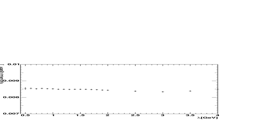
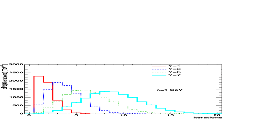
Figure 1: Left: $\lambda$ independence of the GGF. Right: Distribution on the number of iterations needed to calculate the GGF.

In Fig. 2 (left) the growth with energy of the GGF is compared at LL to that at NLL. When higher order corrections are included the intercept diminishes. The bands correspond to the choices of renormalisation scale $\mu=k_{b},k_{b}/2,2k_{b}$, being much narrower at NLL. In Fig. 2 (right) the dependence on the angle between the two external transverse scales, $\vec{k}_{a,b}$, is plotted. The region where this angle is smaller dominates and for larger energies the angular correlation decreases.

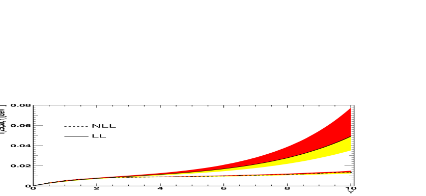
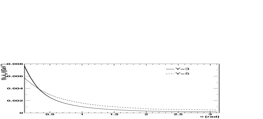
Figure 2: Left: Energy dependence of the GGF. Right: Angular dependence of the GGF.

2.1 Resummation of running coupling terms beyond BFKL

Making use of the regularisation presented in this work it is possible to go beyond the pure BFKL calculation by resumming the running coupling terms. To illustrate this point it is convenient to connect with the work in Ref. [6] where the gluon Regge trajectory was calculated in the context of the renormalisation group evolution of Wilson lines. In Ref. [6] the trajectory is related to the so called “cusp anomalous dimension” in the form

$$\omega_{0}\left(\vec{q},\lambda\right) = -\frac{1}{2}\int_{\lambda^{2}}^{\vec{q}^{2}}\frac{d\vec{k}^{2}}{\vec{k}^{2}}\Gamma_{\rm cusp}\left(\bar{\alpha}_{s}\left(\vec{k}^{2}\right)\right)+{\rm constant},$$ (6)

with $\Gamma_{\rm cusp}\left(\bar{\alpha}_{s}\right)=\bar{\alpha}_{s}+\bar{\alpha}_{s}^{2}{\cal S}$, and ${\cal S}=\frac{1}{3}-\frac{\pi^{2}}{12}+\frac{5}{12}\frac{\beta_{0}}{N_{c}}$. One can then use, as in the original derivation of the NLL BFKL kernel, the ${\cal O}(\alpha_{s}^{2})$ expansion of the coupling, $\bar{\alpha}_{s}\left(\vec{k}^{2}\right)\approx\bar{\alpha}_{s}\left(\mu^{2}\right)-\bar{\alpha}_{s}^{2}\left(\mu^{2}\right)\frac{\beta_{0}}{4N_{c}}\ln{\frac{\vec{k}^{2}}{\mu^{2}}}$, to obtain the result of Eq. (4) by simply fixing the constant of integration to the full calculation of the trajectory in Ref. [2], i.e., ${\rm constant}=\bar{\alpha}_{s}^{2}\frac{3}{2}\zeta(3)$.

The resummation of running coupling terms is then achieved if the resummed running, $\bar{\alpha}_{s}\left(\vec{k}^{2}\right)=1/\frac{\beta_{0}}{4N_{c}}\ln{\frac{\vec{k}^{2}}{\Lambda_{\rm QCD}^{2}}}$, is introduced. With this choice the trajectory reads

$$\omega_{0}\left(\vec{q},\lambda\right) = \frac{4N_{c}}{\beta_{0}}\ln{\frac{\bar{\alpha}_{s}\left(\vec{q}^{2}\right)}{\bar{\alpha}_{s}\left(\lambda^{2}\right)}}+\frac{4N_{c}}{\beta_{0}}{\cal S}\left[\bar{\alpha}_{s}\left(\vec{q}^{2}\right)-\bar{\alpha}_{s}\left(\lambda^{2}\right)\right]+\bar{\alpha}_{s}^{2}\frac{3}{2}\zeta(3).$$ (7)

In this case the $\xi$ function in the real emission is $\xi=\bar{\alpha}_{s}\left(\vec{q}^{2}\right)+\bar{\alpha}_{s}^{2}\left(\vec{q}^{2}\right)\mathcal{S}$, ensuring the $\lambda$ independence of the GGF. This resummation will be further discussed in a coming publication, including a numerical study of the gluon–bremsstrahlung scheme, where the factor $\mathcal{S}$ is absorbed in the coupling constant, together with a comparison to previous approaches in the literature for the treatment of the running [9] and studies of the NLL GGF [10].

3 Conformal spins in N=4 supersymmetric Yang–Mills theory

In the N=4 supersymmetric case [7] the gluon Regge trajectory in this regularisation simplifies to (see Ref. [8] for details)

$$\omega_{0}\left({\vec{q}},\lambda\right) = -a\left\{\ln{\frac{\vec{q}^{2}}{\lambda^{2}}}+\frac{a}{4}\left[\left(\frac{1}{3}-2\xi(2)\right)\ln{\frac{\vec{q}^{2}}{\lambda^{2}}}-6\,\zeta(3)\right]\right\},$$ (8)

where now the coupling $a$ does not run, and double logarithms are not generated in Eq. (8). The expression for

$$\xi \equiv a+a^{2}\left(\frac{1}{12}-\frac{\zeta(2)}{2}\right)$$ (9)

is a simple constant. As the theory is conformally invariant it is possible to find the solution to the NLL BFKL equation first expanding the GGF in conformal spins, $n$, as

$$f\left(\vec{k}_{a},\vec{k}_{b},{\rm Y}\right) = \sum_{n=-\infty}^{\infty}f_{n}\left(|\vec{k}_{a}|,|\vec{k}_{b}|,{\rm Y}\right)e^{in\theta},$$ (10)

and then expressing the coefficients in terms of the known eigenvalues, i.e.,

$$f_{n}\left(|\vec{k}_{a}|,|\vec{k}_{b}|,{\rm Y}\right) = \frac{1}{2\pi|\vec{k}_{a}||\vec{k}_{b}|}\int\frac{d\gamma}{2\pi i}\left(\frac{\vec{k}_{a}^{2}}{\vec{k}_{b}^{2}}\right)^{\gamma-\frac{1}{2}}e^{\omega_{n}(a,\gamma){\rm Y}},$$ (11)

these $\omega_{n}(a,\gamma)$ eigenvalues can be found in [7, 8]. Alternatively, Eq. (11) can be also obtained by means of the iterative method of Eq. (3) by projecting on the conformal spins:

$$f_{n}\left(|\vec{k}_{a}|,|\vec{k}_{b}|,{\rm Y}\right) = \int_{0}^{2\pi}\frac{d\theta}{2\pi}\,f\left(\vec{k}_{a},\vec{k}_{b},{\rm Y}\right)\cos{\left(n\theta\right)}.$$ (12)

The agreement found in Ref. [8] for these projections serves as a cross–check of the calculations in Ref. [7] and shows the accuracy of the method in Eq. (3). This is highlighted in Fig. 3 where the analytic expressions are compared to the iterative ones for the expression in Eq. (11) (left) and the full expansion in Eq. (10) (right).

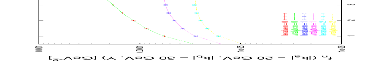
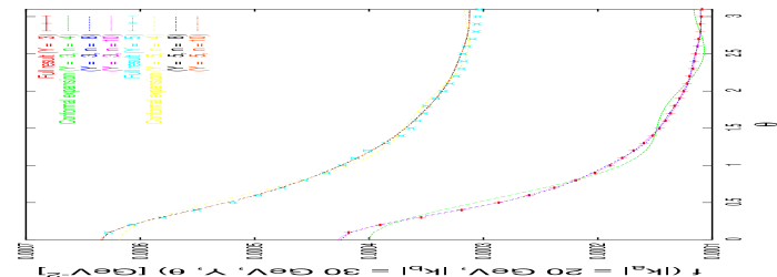
Figure 3: Left: Projection on conformal spins. Right: Convergence to the full GGF as in Eq. (10).

References

• [1] L. N. Lipatov, Sov. J. Nucl. Phys.  23 (1976) 338, E. A. Kuraev, L. N. Lipatov, V. S. Fadin, Sov. Phys. JETP 45 (1977) 199, I. I. Balitsky, L. N. Lipatov, Sov. J. Nucl. Phys.  28 (1978) 822.
• [2] V. S. Fadin, L. N. Lipatov, Phys. Lett. B 429 (1998) 127.
• [3] M. Ciafaloni, G. Camici, Phys. Lett. B 430 (1998) 349.
• [4] J. R. Andersen, A. Sabio Vera, Phys. Lett. B 567 (2003) 116.
• [5] J. R. Andersen, A. Sabio Vera, Nucl. Phys. B 679 (2004) 345.
• [6] I. A. Korchemskaya, G. P. Korchemsky, Phys. Lett. B 387 (1996) 346.
• [7] A. V. Kotikov, L. N. Lipatov, Nucl. Phys. B 582 (2000) 19, Nucl. Phys. B 661 (2003) 19 [Erratum-ibid. B 685 (2004) 405].
• [8] J. R. Andersen, A. Sabio Vera, hep-th/0406009.
• [9] L.N. Lipatov, JETP ${\bf{63}}$, 904 (1986), G. Camici, M. Ciafaloni, Phys. Lett. B ${\bf{395}}$, 118 (1997), R. S. Thorne, Phys. Lett. B 474 (2000) 372, Phys. Rev. D 64 (2001) 074005, J. R. Forshaw, D. A. Ross, A. Sabio Vera, Phys. Lett. B 498 (2001) 149, M. Ciafaloni, D. Colferai, G. P. Salam, A. M. Stasto, Phys. Lett. B 541 (2002) 314, Phys. Rev. D 66 (2002) 054014.
• [10] D.A. Ross, Phys. Lett. B431 (1998) 161, G.P. Salam, JHEP8907 (1998) 19, M. Ciafaloni, D. Colferai, Phys. Lett. B452 (1999) 372, M. Ciafaloni, D. Colferai, G.P. Salam, Phys. Rev. D60 (1999) 114036, R.S. Thorne, Phys. Rev. D60 (1999) 054031, C. R. Schmidt, Phys. Rev. D 60 (1999) 074003, J. R. Forshaw, D. A. Ross, A. Sabio Vera, Phys. Lett. B 455 (1999) 273, G. Altarelli, R. D. Ball, S. Forte, Nucl. Phys. B 575 (2000) 313, Nucl. Phys. B 621 (2002) 359, Nucl. Phys. B 674 (2003) 459, M. Ciafaloni, D. Colferai, G. P. Salam, A. M. Stasto, Phys. Lett. B 576 (2003) 143, Phys. Rev. D 68 (2003) 114003, Phys. Lett. B 587 (2004) 87.