Global analysis of inclusive $B$ decays

Abstract

In light of the large amount of new experimental data, we revisit the determination of $|V_{cb}|$ and $m_{b}$ from inclusive semileptonic and radiative $B$ decays. We study shape variables to order $\Lambda_{\rm QCD}^{3}/m_{b}^{3}$ and $\alpha_{s}^{2}\beta_{0}$, and include the order $\alpha_{s}\,\Lambda_{\rm QCD}/m_{b}$ correction to the hadron mass spectrum in semileptonic decay, which improves the agreement with the data. We focus on the $1S$ and kinetic mass schemes for the $b$ quark, with and without expanding $m_{b}-m_{c}$ in HQET. We perform fits to all available data from BABAR, BELLE, CDF, CLEO, and DELPHI, discuss the theoretical uncertainties, and compare with earlier results. We find $|V_{cb}|=\left(41.4\pm 0.6\pm 0.1_{\tau_{B}}\right)\times 10^{-3}$ and $m_{b}^{1S}=4.68\pm 0.03\,\text{GeV}$, including our estimate of the theoretical uncertainty in the fit.

I Introduction

In the last few years there has been intense theoretical and experimental activity directed toward a precise determination of the Cabibbo-Kobayashi-Maskawa (CKM) matrix element $|V_{cb}|$ from combined fits to inclusive semileptonic $B$ decay distributions Bauer:2002sh ; delphifit ; Mahmood:2002tt ; Aubert:2004aw . The idea is that using the operator product expansion (OPE), sufficiently inclusive observables can be predicted in terms of $|V_{cb}|$, the $b$ quark mass, $m_{b}$, and a few nonperturbative matrix elements that enter at order $\Lambda_{\rm QCD}^{2}/m_{b}^{2}$ and higher orders. One then extracts these parameters and $|V_{cb}|$ from shapes of $B$ decay spectra and the semileptonic $B$ decay rate. This program also tests the consistency of the theory and the accuracy of the theoretical predictions for inclusive decay rates. This is important also for the determination of $|V_{ub}|$, whose error is a major uncertainty in the overall constraints on the unitarity triangle.

The OPE shows that in the $m_{b}\gg\Lambda_{\rm QCD}$ limit inclusive $B$ decay rates are equal to the $b$ quark decay rates OPE ; book , and the corrections are suppressed by powers of $\alpha_{s}$ and $\Lambda_{\rm QCD}/m_{b}$. High-precision comparison of theory and experiment requires a precise determination of the heavy quark masses, as well as the nonperturbative matrix elements that enter the expansion. These are $\lambda_{1,2}$, which parameterize the nonperturbative corrections to inclusive observables at ${\cal O}(\Lambda_{\rm QCD}^{2}/m_{b}^{2})$. At order $\Lambda_{\rm QCD}^{3}/m_{b}^{3}$, six new matrix elements occur, usually denoted by $\rho_{1,2}$ and ${\cal T}_{1,2,3,4}$.

In this paper, we perform a global fit to the available inclusive decay observables from BABAR, BELLE, CDF, CLEO, and DELPHI, including theoretical expressions computed to order $\alpha_{s}^{2}\beta_{0}$, $\alpha_{s}\Lambda_{\rm QCD}/m_{b}$ and $\Lambda_{\rm QCD}^{3}/m_{b}^{3}$. A potential source of uncertainty in the OPE predictions is the size of possible violations of quark-hadron duality NIdual . Studying $B$ decay distributions is the best way to constrain these effects experimentally, since it should influence the relationship between shape variables of different spectra. We find that at the current level of precision, there is excellent agreement between theory and experiment, with no evidence for violations of duality in inclusive $b\to c$ decays.

A previous analysis of the experimental data was presented in 2002 Bauer:2002sh . There has been considerable new data since then, which has been included in the present analysis, and reduces the errors on $|V_{cb}|$ and $m_{b}$. In addition, the $\alpha_{s}\Lambda_{\rm QCD}/m_{b}$ corrections to the hadronic invariant mass spectrum as a function of the lepton energy cut have now been computed Trott:2004xc , and are included in the present analysis. This reduces the theoretical uncertainty on the hadronic mass moments. We also compare our results with other recent analyses Gambino:2004qm ; delphifit ; Aubert:2004aw .

II Possible Schemes

The inclusive $B$ decay spectra depend on the masses of the $b$ and $c$ quarks, which can be treated in many different ways. The $b$ quark is treated as heavy, and theoretical computations for $B^{(*)}$ decays are done as an expansion in powers of $\Lambda_{\rm QCD}/m_{b}$. The use of the $1/m_{b}$ expansion is common to all methods.

The decay rates for $B\to X_{c}$ decay depend on the mass of the $c$ quark, for example, through its effect on the decay phase space. One can treat the $c$ quark as a heavy quark. This allows one to compute the $D^{(*)}$ meson masses as an expansion in powers of $\Lambda_{\rm QCD}/m_{c}$. The observed $D^{(*)}$ masses can be used to determine $m_{c}$. Since the computations are performed to $\Lambda_{\rm QCD}^{3}/m_{c}^{3}$, this introduces errors of fractional order $\Lambda_{\rm QCD}^{4}/m_{c}^{4}$ in $m_{c}$, which gives fractional errors of order $\Lambda_{\rm QCD}^{4}/(m_{b}^{2}m_{c}^{2})$ in the inclusive $B$ decay rates, since charm mass effects first enter at order $m_{c}^{2}/m_{b}^{2}$. In this method, one starts with the parameters $|V_{cb}|$, $m_{b}$, $m_{c}$, $\lambda_{1,2}$, $\rho_{1,2}$ and ${\cal T}_{1-4}$. The $B^{*}-B$, $D^{*}-D$ and $B-D$ mass differences can be used to eliminate $m_{b}-m_{c}$, $\lambda_{2}$ and $\rho_{2}$. Only mass differences are used to avoid introducing the parameter $\bar{\Lambda}$ of order $\Lambda_{\rm QCD}$; thus we do not use the $B$ meson mass to eliminate $m_{b}$. Three linear combinations of the four ${\cal T}_{i}$’s occur in inclusive $B$ decays, and the remaining linear combination would be needed for inclusive $B^{*}$ decays. In summary the parameters used are (i) $|V_{cb}|$; (ii) one parameter of order the quark mass: $m_{b}$; (iii) one parameter of order $\Lambda_{\rm QCD}^{2}$: $\lambda_{1}$; and (iv) four parameters of order $\Lambda_{\rm QCD}^{3}$: $\rho_{1}$, ${\cal T}_{1}-3{\cal T}_{4}$, ${\cal T}_{2}+{\cal T}_{4}$, ${\cal T}_{3}+3{\cal T}_{4}$. These seven parameters are determined by a global fit to moments of the $B$ decay distributions, and the semileptonic branching ratio. This is the procedure used in Ref. Bauer:2002sh .

An alternative approach is to avoid using the $1/m_{c}$ expansion for the charm quark Gambino:2004qm , since it introduces $\Lambda_{\rm QCD}/m_{c}$ corrections, which are larger than the $\Lambda_{\rm QCD}/m_{b}$ corrections of the $1/m_{b}$ expansion. In this case heavy quark effective theory (HQET) can no longer be used for the $c$ quark system, and there are no constraints on $m_{c}$ from the $D$ and $D^{*}$ meson masses. At the same time, it is not necessary to expand heavy meson states in an expansion in $1/m_{b,c}$, so that the time-ordered products ${\cal T}_{1-4}$ can be dropped. With this procedure, one has in addition to (i) $|V_{cb}|$; (ii) two parameters of order the quark mass: $m_{b,c}$; (iii) two parameters of order $\Lambda_{\rm QCD}^{2}$: $\lambda_{1,2}$; and (iv) two parameters of order $\Lambda_{\rm QCD}^{3}$: $\rho_{1,2}$. The number of parameters is the same whether or not one expands in $1/m_{c}$. If one does not expand, two parameters of order $\Lambda_{\rm QCD}^{3}$ are replaced by two lower order parameters, one of order the quark mass, and one of order $\Lambda_{\rm QCD}^{2}$. The expansion parameters, such as $\lambda_{1,2}$ are not the same in the two approaches. The values of $\lambda_{1,2}$ not expanding the states in $1/m_{Q}$ are the values of $\lambda_{1,2}$ plus various time-ordered products ${\cal T}_{1}-{\cal T}_{4}$ when one expands the states in powers of $1/m_{Q}$.

In addition to the choice of expanding or not expanding in $1/m_{c}$, one also has a choice of possible quark mass schemes. It has long been known that a “threshold mass” definition for $m_{b}$ is preferred over both the pole and the $\overline{\rm MS}$ schemes, and it was shown in Ref. Bauer:2002sh that the expansions are indeed better behaved in the $1S$ ups1 ; ups2 or PS 3loopPS schemes for $m_{b}$. If one expands in $1/m_{c}$, then $m_{c}$ is eliminated through use of the meson masses, and does not enter the final results. If one does not expand in $1/m_{c}$, then $m_{c}$ is a fit parameter. In this method, $m_{c}$ is treated as much lighter than $m_{b}$, so the charm quark mass is chosen to be $\overline{m}_{c}(\mu)$, the $\overline{\rm MS}$ mass renormalized at a scale $\mu\sim m_{b}$. This is similar to how strange quark mass effects could be included in $B\to X_{s}\gamma$ decay. In our computation, we will choose the scale $\mu=m_{b}$.

In addition to the $1S$, PS, pole and $\overline{\rm MS}$ schemes, we have also used the kinetic scheme mass for the $b$-quark, $m_{b}^{\rm kin}(\mu)$, renormalized at a low scale $\mu\sim 1\,$GeV. The scale $\mu$ enters the definition of the kinetic mass, and should not be confused with the scale parameter in dimensional regularization. The relation between the pole and kinetic masses is computed as a perturbative expansion in powers of $\alpha_{s}(\mu)$, so one cannot make $\mu$ too small. In the kinetic scheme Gambino:2004qm the definitions $\mu_{\pi}^{2}=-\lambda_{1}+{\cal O}(\alpha_{s})$, $\mu_{G}^{2}=3\lambda_{2}$, $\rho_{D}^{3}=\rho_{1}+{\cal O}(\alpha_{s})$, and $\rho_{\rm LS}^{3}=3\rho_{2}$ are used.

One cannot decide which scheme is best by counting parameters, or by assuming that not expanding in $1/m_{c}$ is better than expanding in $1/m_{c}$. Ultimately, what matters is the accuracy to which experimentally measured quantities can be reliably computed with currently available techniques. For example, full QCD has two parameters, $m_{b}$ and $m_{c}$, which can be fixed using the $B$ and $D$ meson masses. [Unfortunately, this is not possible to less than 1% precision at the present time.] Then one can predict all inclusive $B$ decays, as well as the $B^{*}$ and $D^{*}$ masses with no parameters. This would be the “best” method to use — unfortunately, we cannot accurately compute the desired quantities reliably in QCD. At present, it is better to use the HQET expansion in $1/m_{b}$ and $1/m_{c}$, with 6 parameters, and compute to order $1/m_{Q}^{3}$. In the (distant) future, it could well be that using full QCD, with no parameters, is the best method to use.

We have done a fit to the experimental data using 11 schemes: the $1S$, PS, pole, $\overline{\rm MS}$ and kinetic schemes expanding in $1/m_{c}$, not expanding in $1/m_{c}$ and using $\overline{m}_{c}(m_{b})$, and finally, not expanding in $1/m_{c}$ and using the kinetic scheme for both $m_{b}$ and $m_{c}$. In addition, the PS and kinetic schemes introduce a scale $\mu$, which is sometimes called the factorization scale. We have also examined the factorization scale dependence which is present in these two schemes. We confirm the conclusions of Ref. Bauer:2002sh , that the pole and $\overline{\rm MS}$ schemes are significantly worse than the threshold mass schemes, as expected theoretically. This holds regardless of whether or not one expands in $1/m_{c}$. We recommend that these schemes be avoided for high precision fits to inclusive $B$ decays. We also find that the PS scheme gives results comparable to those of the $1S$ scheme (both expanding and not expanding in $1/m_{c}$), and that the PS scheme results do not significantly depend on the choice of factorization scale. We compared the PS scheme with the 1S scheme in Ref. Bauer:2002sh , and do not repeat the results here.

Based on the above discussion, we present our results in five different mass schemes, using:

(6)

Schemes $1S_{\text{EXP}}$ and $\mbox{kin}_{\text{EXP}}$ contain time ordered products at order $\Lambda_{\rm QCD}^{3}/m_{b}^{3}$, while they are absent from $1S_{\text{NO}}$, $\mbox{kin}_{\text{NO}}$, and $\mbox{kin}_{\text{UG}}$. As discussed, the latter three schemes have the charm quark mass as an additional parameter at leading order in $\Lambda_{\rm QCD}/m_{b}$. Scheme $1S_{\text{EXP}}$ is that used in Ref. Bauer:2002sh , while scheme $\mbox{kin}_{\text{UG}}$ is that used in Ref. Gambino:2004qm .

III Shape variables and the data

We study three different distributions, the charged lepton energy spectrum volo ; gremmetal ; GK ; GS and the hadronic invariant mass spectrum FLSmass1 ; FLSmass2 ; GK ; Trott:2004xc in semileptonic $B\to X_{c}\ell\bar{\nu}$ decays, and the photon spectrum in $B\to X_{s}\gamma$ FLS ; kl ; llmw ; bauer . The theoretical predictions for these (as well as for the semileptonic $B\to X_{c}\ell\bar{\nu}$ rate LSW ) are known to order $\alpha_{s}^{2}\beta_{0}$ and $\Lambda_{\rm QCD}^{3}/m_{b}^{3}$, where $\beta_{0}=11-2n_{f}/3$ is the coefficient of the first term in the QCD $\beta$-function. For the $B\to X\ell\bar{\nu}$ branching rate, we use the average of the $B^{\pm}$ and $B^{0}$ data as quoted in the PDG pdg ,

$${\cal B}(B\to X\ell\bar{\nu}) = 10.73\pm 0.28\,\%.$$ (8)

We apply a relative $-2\%$ correction to ${\cal B}(B\to X\ell\bar{\nu})$ to account for the $B\to X_{u}\ell\bar{\nu}$ fraction, and so use

$${\cal B}(B\to X_{c}\ell\bar{\nu}) = 0.98\ {\cal B}(B\to X\ell\bar{\nu}).$$ (9)

The uncertainty of $|V_{ub}|$ is not a dominant error in ${\cal B}(B\to X_{c}\ell\bar{\nu})$. The fit result for $|V_{cb}|$ depends not only on ${\cal B}(B\to X_{c}\ell\bar{\nu})$, but also on the partial semileptonic branching ratios measured by the BABAR Collaboration Aubert:2004td , which have smaller errors than Eq. (8). The published BABAR results have already been corrected for $B\to X_{u}\ell\bar{\nu}$ contamination.

III.1 Lifetime

The value of $|V_{cb}|$ depends on the $B$ meson lifetimes. The ratio of $B^{+}$ and $B^{0}$ lifetimes is $\tau_{+}/\tau_{0}=1.086\pm 0.017$ pdg . Isospin violation in the $B$ meson semileptonic width is expected to be smaller than both $\tau_{+}/\tau_{0}$ and the uncertainties in the current analysis. The $\approx 8$% isospin violation in the lifetimes is probably due to the nonleptonic decay channels.

An additional source of isospin violation in the experimental measurements is through the production rates of $B^{+}$ and $B^{0}$ mesons, which is expected to be of the order of a few percent to perhaps as large as 10% kaiser . Let $f_{+}$ and $f_{0}$ be the fraction of $B^{+}$ and $B^{0}$ mesons produced in $\Upsilon(4S)$ decay, with $f_{+}+f_{0}=1$. Then the measured semileptonic branching ratios are

$${\cal B} = f_{+}{\Gamma_{\text{sl}}\over\Gamma_{\text{sl}}+\Gamma_{\text{nl},+}}+f_{0}{\Gamma_{\text{sl}}\over\Gamma_{\text{sl}}+\Gamma_{\text{nl},0}}$$ (10)

where ${\cal B}$ and $\Gamma_{\text{sl}}$ are computed with the same lepton energy cut. In writing Eq. (10), we have used the fact that isospin violation in the semileptonic rates is small, so that the same value for $\Gamma_{\text{sl}}$ is used for both $B^{+}$ and $B^{0}$.

The measured semileptonic branching ratios can thus be written as

$${\cal B} = \tau_{\text{eff}}\ \Gamma_{\text{sl}}$$ (11)

in terms of the effective lifetime

$$\tau_{\text{eff}} = f_{+}\tau_{+}+f_{0}\tau_{0}.$$ (12)

One can rewrite this as

$$\tau_{\text{eff}} = {\tau_{+}+\tau_{0}\over 2}+{(f_{+}-f_{0})(\tau_{+}-\tau_{0})\over 2}.$$ (13)

Using the PDG 2004 lifetime values, and the measured $f_{+}/f_{0}$ ratio isospin gives

$$\tau_{\text{eff}} = 1.60\pm 0.01\ \text{ps}$$ (14)

where the contribution from the second term in Eq. (13) is negligible to both the value and the error.

III.2 Lepton Moments

For the charged lepton energy spectrum we define the integrals

$$R_{n}(E_{\rm cut},\mu)=\int_{E_{\rm cut}}\left(E_{\ell}-\mu\right)^{n}\,{{\rm d}\Gamma\over{\rm d}E_{\ell}}\,{\rm d}E_{\ell}\,,$$ (15)

where ${\rm d}\Gamma/{\rm d}E_{\ell}$ is the spectrum in the $B$ rest frame and $E_{\rm cut}$ is a lower cut on the lepton energy. Moments of the lepton energy spectrum with a lepton energy cut $E_{\rm cut}$ are given by

$$\left\langle E_{\ell}^{n}\right\rangle_{E_{\rm cut}}={R_{n}(E_{\rm cut},0)\over R_{0}(E_{\rm cut},0)}\,,$$ (16)

and central moments by

$$\left\langle\left(E_{\ell}-\left\langle E_{\ell}\right\rangle\right)^{n}\right\rangle_{E_{\rm cut}}={R_{n}(E_{\rm cut},\left\langle E_{\ell}\right\rangle_{E_{\rm cut}})\over R_{0}(E_{\rm cut},0)}\,,$$ (17)

which can be determined as a linear combination of the non-central moments.

The BABAR Collaboration Aubert:2004td measured the partial branching fraction $\tau_{B}R_{0}(E_{\rm cut},0)$, the mean lepton energy $\left\langle E_{\ell}\right\rangle_{E_{\rm cut}}$, and the second and third central moments $\left\langle\left(E_{\ell}-\left\langle E_{\ell}\right\rangle\right)^{n}\right\rangle_{E_{\rm cut}}$ for $n=2,3$, each for lepton energy cuts of $E_{\rm cut}=0.6,\ 0.8,\ 1.0,\ 1.2$, and $1.5$ GeV.

The BELLE Collaboration Abe:2004zv measured the mean lepton energy and the second central moment for lepton energy cuts of $E_{\rm cut}=0.6,\ 0.8,\ 1.0,\ 1.2$, and $1.5$ GeV.

The CLEO Collaboration Mahmood:2002tt ; Mahmood:2004kq measured the mean lepton energy and second central moment (variance) for $E_{\rm cut}=0.7-1.6$ GeV in steps of $0.1$ GeV.

The DELPHI Collaboration DELPHIdata measured the mean lepton energy, and the $n=2,3$ central moments, all with no energy cut.

In total, we have 53 experimental quantities from the lepton moments, 20 from BABAR, 10 from BELLE, 20 from CLEO, and 3 from DELPHI.

III.3 Hadron Moments

For the $B\to X_{c}\ell\bar{\nu}$ hadronic invariant mass spectrum, we define

$$\langle m_{X}^{2n}\rangle_{E_{\rm cut}}={\displaystyle\int_{E_{\rm cut}}(m_{X}^{2})^{n}\,{{\rm d}\Gamma\over{\rm d}m_{X}^{2}}\,{\rm d}m_{X}^{2}\over\displaystyle\int_{E_{\rm cut}}{{\rm d}\Gamma\over{\rm d}m_{X}^{2}}\,{\rm d}m_{X}^{2}}\,,$$ (18)

where $E_{\rm cut}$ is again the cut on the lepton energy. Sometimes $\overline{m}_{D}^{2}\equiv[(m_{D}+3m_{D^{*}})/4]^{2}$ is subtracted out in the definitions, $\langle(m_{X}^{2}-\overline{m}_{D}^{2})^{n}\rangle$, or the measurements of the normal moments are quoted, $\langle(m_{X}^{2}-\langle m_{X}^{2}\rangle)^{n}\rangle$, but these can easily be computed from $\langle m_{X}^{2n}\rangle$.

The BABAR Collaboration Aubert:2004te measured the mean values of $m_{X}$, $m_{X}^{2}$, $m_{X}^{3}$ and $m_{X}^{4}$ (i.e., $n=1/2,\ 1,\ 3/2,\ 2$ moments) for lepton energy cuts $E_{\rm cut}=0.9-1.6$ GeV in steps of $0.1$ GeV.

The BELLE Collaboration Abe:2004ks measured the mean values of $m_{X}$ and $m_{X}^{2}$ for lepton energy cuts $E_{\rm cut}=0.9-1.6$ GeV in steps of $0.1$ GeV.

The CDF Collaboration cdfhadron measured the mean value of $m_{X}^{2}$ and its variance, with a lepton energy cut $E_{\rm cut}=0.7$ GeV.

The CLEO Collaboration Csorna:2004kp measured the mean value of $m_{X}^{2}-\overline{m}_{D}^{2}$ and the variance of $m_{X}^{2}$ for lepton energy cuts of $1.0$ and $1.5$ GeV.

The DELPHI Collaboration DELPHIdata measured the mean value of $m_{X}^{2}-\overline{m}_{D}^{2}$, $(m_{X}^{2}-\overline{m}_{D}^{2})^{2}$, the variance of $m_{X}^{2}$, and the third central moment of $m_{X}^{2}$, all with no energy cut.

Recently half-integer moments of the $m_{X}^{2}$ spectrum Gambino:2004qm ; Trott:2004xc have received some attention. While non-integer moments of the lepton energy spectrum have been computed in a power series in $1/m_{b}$ BT , this is not true for fractional moments of the $m_{X}^{2}$ spectrum. In Gambino:2004qm ; Trott:2004xc expressions for the half-integer moments were proposed which involve expansions that were claimed to be in powers of $\Lambda_{\rm QCD}/m_{c}$. However, in the limit $m_{c}\ll m_{b}$ (i.e., $m_{c}$ of order $\sqrt{m_{b}\Lambda_{\rm QCD}}$ or less), the higher order terms in these expansion scale with powers of $m_{b}\Lambda_{\rm QCD}/m_{c}^{2}$, which in this limit is of order unity or larger. On the other hand, in the small velocity limit, $m_{b}\sim m_{c}\gg m_{b}-m_{c}\gg\Lambda_{\rm QCD}$, the expansion of $\langle m_{X}^{2n+1}\rangle$ is well-behaved. Thus, the calculations of the half-integer moments as presented in Gambino:2004qm ; Trott:2004xc do not correspond to a power series in $1/m_{b,c}$ in the $m_{c}\ll m_{b}$ limit and omitted terms are only power suppressed in the small velocity limit. In addition, the BLM corrections to these moments are currently unknown, because they require the BLM contribution from the virtual terms, which have not been computed. For these reasons we will not use these half-integer moments in the fit, but will compare the fit results with the measured values. Omitting the half-integer moments, there are 16 data points from BABAR, 8 from BELLE, 2 from CDF, 4 from CLEO, and 4 from DELPHI, for a total of 34 measurements.

III.4 Photon Spectrum

For $B\to X_{s}\gamma$, we define

$$\langle E_{\gamma}^{n}\rangle_{E_{\rm cut}}={{\displaystyle\int_{E_{\rm cut}}E_{\gamma}^{n}\,{{\rm d}\Gamma\over{\rm d}E_{\gamma}}\,{\rm d}E_{\gamma}}\over{\displaystyle\int_{E_{\rm cut}}{{\rm d}\Gamma\over{\rm d}E_{\gamma}}\,{\rm d}E_{\gamma}}}\,,$$ (19)

where ${\rm d}\Gamma/{\rm d}E_{\gamma}$ is the photon spectrum in the $B$ rest frame, and $E_{\rm cut}$ is the photon energy cut. In this case the variance, $\langle(E_{\gamma}-\langle E_{\gamma}\rangle)^{2}\rangle=\langle E_{\gamma}^{2}\rangle-\langle E_{\gamma}\rangle^{2}$, is often used instead of the second moment, and higher moments are not used as they are very sensitive to the boost of the $B$ meson in the $\Upsilon$ rest frame (though this is absent if ${\rm d}\Gamma/{\rm d}E_{\gamma}$ is reconstructed from a measurement of ${\rm d}\Gamma/{\rm d}E_{m_{X_{s}}}$) and to the details of the shape function. $\langle E_{\gamma}^{n}\rangle$ are known to order $\alpha_{s}^{2}\beta_{0}$ llmw and $\Lambda_{\rm QCD}^{3}/m_{b}^{3}$ bauer . These moments are expected to be described by the OPE once $m_{B}/2-E_{\rm cut}\gg\Lambda_{\rm QCD}$. Precisely how low $E_{\rm cut}$ has to be to trust the results can only be decided by studying the data as a function of $E_{\rm cut}$; one may expect that $E_{\rm cut}=1.8\,\mbox{GeV}$ available at present Koppenburg:2004fz is sufficient. Note that the perturbative corrections included are sensitive to the $m_{c}$-dependence of the $b\to c\bar{c}s$ four-quark operator ($O_{2}$) contribution. This is a particularly large effect in the $O_{2}-O_{7}$ interference llmw , but its relative influence on the moments of the spectrum is less severe than that on the total decay rate.

We use the BELLE Koppenburg:2004fz , and CLEO cleophoton measurements of the mean photon energy and variance, with photon energy cuts of $1.8$ and $2.0$ GeV, respectively, and the BABAR measurement Aubert:2002pb of the mean photon energy with a cut of $2.094$ GeV for a total of 5 measurements.

IV Fit Procedure

As discussed in Sec. II, there are many ways to treat the quark masses and hadronic matrix elements that occur in the OPE results for the spectra. In the schemes where $m_{b}-m_{c}$ is expanded in HQET (such as $1S_{\text{EXP}}$ and $\mbox{kin}_{\text{EXP}}$), the theoretical expressions for the shape variables defined in Eqs. (15), (18), and (19) include 17 terms

$$X_{E_{\rm cut}} = X^{(1)}+X^{(2)}\,\Lambda+X^{(3)}\,\Lambda^{2}+X^{(4)}\,\Lambda^{3}+X^{(5)}\,\lambda_{1}$$

$$+ X^{(6)}\,\lambda_{2}+X^{(7)}\,\lambda_{1}\Lambda+X^{(8)}\,\lambda_{2}\Lambda+X^{(9)}\,\rho_{1}$$

$$+ X^{(10)}\,\rho_{2}+X^{(11)}\,{\cal T}_{1}+X^{(12)}\,{\cal T}_{2}+X^{(13)}\,{\cal T}_{3}$$

$$+ X^{(14)}\,{\cal T}_{4}+X^{(15)}\,\epsilon+X^{(16)}\,\epsilon^{2}_{\rm BLM}+X^{(17)}\,\epsilon\,\Lambda\,,$$

while in the schemes when $m_{c}$ is treated as an independent free parameter (such as $1S_{\text{NO}}$, $\mbox{kin}_{\text{NO}}$, and $\mbox{kin}_{\text{UG}}$), we have 22 terms

$$Y_{E_{\rm cut}} = Y^{(1)}+Y^{(2)}\,\Lambda+Y^{(3)}\,\Lambda_{c}+Y^{(4)}\,\Lambda^{2}+Y^{(5)}\,\Lambda\Lambda_{c}$$ (21)

$$+ Y^{(6)}\,\Lambda_{c}^{2}+Y^{(7)}\,\Lambda^{3}+Y^{(8)}\,\Lambda^{2}\Lambda_{c}+Y^{(9)}\,\Lambda\Lambda_{c}^{2}$$

$$+ Y^{(10)}\,\Lambda_{c}^{3}+Y^{(11)}\,\lambda_{1}+Y^{(12)}\,\lambda_{2}+Y^{(13)}\,\lambda_{1}\Lambda$$

$$+ Y^{(14)}\,\lambda_{2}\Lambda+Y^{(15)}\,\lambda_{1}\Lambda_{c}+Y^{(16)}\,\lambda_{2}\Lambda_{c}+Y^{(17)}\,\rho_{1}$$

$$+ Y^{(18)}\,\rho_{2}+Y^{(19)}\,\epsilon+Y^{(20)}\,\epsilon^{2}_{\rm BLM}+Y^{(21)}\,\epsilon\,\Lambda$$

$$+ Y^{(22)}\,\epsilon\,\Lambda_{c}\,.$$

In Eqs. (IV) and (21) $\Lambda$ and $\Lambda_{c}$ are respectively the differences between the $b$ and $c$ quark masses and their reference values about which we expand. The coefficients $X^{(k)}$ and $Y^{(k)}$ are functions of $E_{\rm cut}$, and ($X_{E_{\rm cut}}$, $Y_{E_{\rm cut}}$) are any of the experimental observables discussed earlier. The parameter $\epsilon\equiv 1$ counts powers of $\alpha_{s}$. We have used $\alpha_{s}(m_{b})=0.22$. The strong coupling constant is not a free parameter, but is determined from other measurements such as the hadronic width of the $Z$. The hadron and lepton moments are integrals of the same triple differential decay rate with different weighting factors. The use of different values of $\alpha_{s}$ for the hadron and lepton moments, as done in Ref. Gambino:2004qm , is an ad hoc choice.

V The Fit

We use the program MINUIT to perform a global fit to all observables introduced in Sec. III in each of the 11 schemes mentioned in Sec. II. There are a total of 92 lepton, hadron, and photon moments, plus the semileptonic width, to be fit using 7 parameters, so the fit has $\nu=86$ degrees of freedom.

To evaluate the $\chi^{2}$ required for the fit, we include both experimental and theoretical uncertainties. For the experimental uncertainties we use the full correlation matrix for the observables from a given differential spectrum as published by the experimental collaborations. In addition to these experimental uncertainties there are theoretical uncertainties, which correspond to how well we expect to be able to compute each observable theoretically. For a given observable, our treatment of theoretical uncertainties is similar to that in Ref. Bauer:2002sh .

It is important to include theoretical uncertainties in the fit, since not all quantities can be computed with the same precision. We have treated theoretical errors as though they have a normal distribution with zero mean, and standard deviation equal to the error estimate. Strictly speaking, the theoretical formula has some definite higher order correction, which is at present unknown. One can then view the normal distribution used for the theory value as the prior distribution in a Bayesian analysis. The way in which theoretical errors are included is a matter of choice, and there is no unique prescription.

We now discuss in detail the theoretical uncertainties included in the fit. Those who find this procedure abhorrent can skip the entire discussion, since we will also present results not including theory errors.

V.1 Theory uncertainties

Theoretical uncertainties in inclusive observables as discussed here originate from four main sources. First, there are uncertainties due to uncalculated power corrections. For schemes $1S_{\text{EXP}}$ and $\mbox{kin}_{\text{EXP}}$, these are of order $\Lambda_{\rm QCD}^{4}/(m_{b}^{2}m_{c}^{2})\sim 0.001$, while for schemes $1S_{\text{NO}}$ and $\mbox{kin}_{\text{NO}}$ where no $1/m_{c}$ expansion is performed, these are of order $\Lambda_{\rm QCD}^{4}/m_{b}^{4}\sim 0.0001$. Next, there are uncertainties due to uncalculated higher order perturbative terms. In particular, the full two loop result proportional to $\alpha_{s}^{2}/(4\pi)^{2}\sim 0.0003$ is not available. An alternative way to estimate these perturbative uncertainties is by the size of the smallest term computed in the series, which is the term proportional to $\alpha_{s}^{2}\beta_{0}$. We choose here to use half of this last computed term as an estimate of the uncertainty. There are also uncalculated effects of order $(\alpha_{s}/4\pi)\Lambda_{\rm QCD}^{2}/m_{b}^{2}\sim 0.0002$. Finally, there is an uncertainty originating from effects not included in the OPE in the first place. Such effects sometimes go under the name “duality violation,” and are very hard to quantify. For this reason, we do not include an explicit contribution to the overall theoretical uncertainty from such effects. If duality violation would be larger than the other theoretical uncertainties they would give rise to a poor fit to the data. To determine the uncertainties for dimensionful quantities such as the moments considered here, we have to multiply these numbers by the appropriate dimensionful quantity. This number is obtained from dimensional analysis, and we use for the $n$’th hadronic moment $(m_{B}^{2})^{n}f_{n}$, while we use $(m_{B}/2)^{n}f_{n}$ for the $n$’th leptonic moment. The factors $f_{n}$ are chosen to be $f_{0}=f_{1}=1$, $f_{2}=1/4$ and $f_{3}=1/(6\sqrt{3})$. The values for $f_{2}$ and $f_{3}$ are the maximum allowed values for the second and third central moments (variance and skewness) for a probability distribution on the interval $[0,1]$.

The complete BLM piece has not been computed for the non-integer hadronic moments. The perturbative uncertainty is therefore dominated by this contribution of order $\beta_{0}\alpha_{s}^{2}/(4\pi)^{2}\sim 0.003$. We will use $A\sim 0.003$ for the non-integer hadronic moments when we compare experiment with theory.

For the hadronic mass and lepton energy moments, which depend on the value of the cut on the lepton energy, we have to decide how to treat the correlation of the theoretical uncertainties. In the global fit by the BABAR Collaboration Aubert:2004aw , the theory errors for a given observable with different cuts on $E_{\ell}$ were treated as 100% correlated. This ignores the fact that the higher order terms omitted in the OPE depend on the lepton energy cut. In Ref. Bauer:2002sh , only the two extreme values of the lepton energy cut were included in the fit, and the correlation of the theory uncertainties was neglected. Here we take the correlation of the theoretical uncertainties to be given by the correlation between the experimental measurements, which captures the correlations due to the fact that observables with different cuts share some common events.

For the photon energy moments an additional source of uncertainty is the fact that the presence of any experimentally sensible value for $E_{\rm cut}$ affects the mean photon energy $\left\langle E_{\gamma}\right\rangle$ such that the extracted value of $m_{b}$ is biased toward larger values because of shape function effects bauer . However, this shift cannot be calculated model independently. Rather than include a model dependence, we have multiplied the theory uncertainties for the $b\to s\gamma$ rates by the ratios of the energy difference from the endpoint, relative to that for BELLE with $E_{\rm cut}=1.8$ GeV.

To summarize, we define the combined experimental and theoretical error matrix for a given observable to be

$$\sigma^{2}_{ij}=\sigma_{i}\,\sigma_{j}\,c_{ij}\,,\qquad\text{no\ sum on}\ i,j\,,$$ (22)

where $i$ and $j$ denote observables, $c_{ij}$ is the experimental correlation matrix, and

$$\sigma_{i} = \sqrt{(\sigma^{\rm exp}_{i})^{2}+\left(A\,f_{n}m_{B}^{2n}\right)^{2}+\left({B_{i}}/{2}\right)^{2}}$$

for the n’th hadron moment ,

$$\sigma_{i} = \sqrt{(\sigma^{\rm exp}_{i})^{2}+\left(A\,f_{n}{(m_{B}/2)^{n}}\right)^{2}+\left({B_{i}}/{2}\right)^{2}}$$

for the n’th lepton moment ,

$$\sigma_{i} = \sqrt{(\sigma^{\rm exp}_{i})^{2}+\left(A\,f_{n}{(m_{B}/2)^{n}}\right)^{2}+\left({B_{i}}/{2}\right)^{2}}$$ (23)

for the n’th photon moment ,

and $f_{0}=f_{1}=1$, $f_{2}=1/4$, $f_{3}=1/(6\sqrt{3})$. Here $\sigma^{\rm exp}_{i}$ are the experimental errors, $B_{i}=X^{(16)}$ or $Y^{(20)}$ are the coefficients of the last computed terms in the perturbation series, and $A$ contains the errors discussed earlier. We take $A=0.001$ for the data used in the fit, except for the CLEO and BABAR photon moments, where we multiply $A$ by $1.3$ and $1.5$, respectively, to account for the increase in shape function effects as one limits the allowed region of the photon spectrum.

We stress that there is no unique way to estimate theoretical uncertainties to a given expression. Thus, while we believe that our estimates are reasonable, it is certainly not the only possible way to estimate the theory uncertainties (e.g., taking the theory correlation to be identical to the experimental correlations is just an educated guess).

V.2 Experimental correlations

Some of the experimental correlation matrices have negative eigenvalues. In some cases, these are at the level of round-off errors. To avoid these negative values, we have added $0.01$ to the diagonal entries for the correlation matrices for the BABAR and CLEO lepton moments, and the DELPHI hadron moments.

The correlation matrix for the BABAR hadronic moments Aubert:2004aw contains negative eigenvalues which are much larger than any round-off uncertainties. This persists even if only every second value of the cut is used, as advocated in Aubert:2004aw , so we are forced to add $0.05$ to the diagonal entries of the correlation matrix for the BABAR hadron moments to make the eigenvalues positive. Note that the correlation matrix can have negative eigenvalues only if the probability distribution can take on negative values.

The preliminary correlation matrix for the BELLE lepton and hadron moments was used in the fit belleprivate .

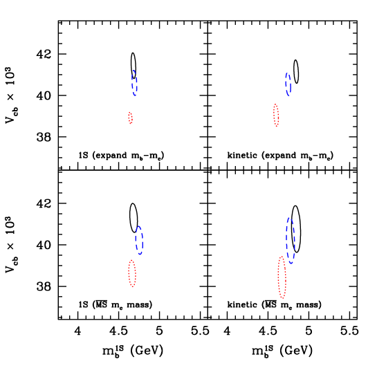
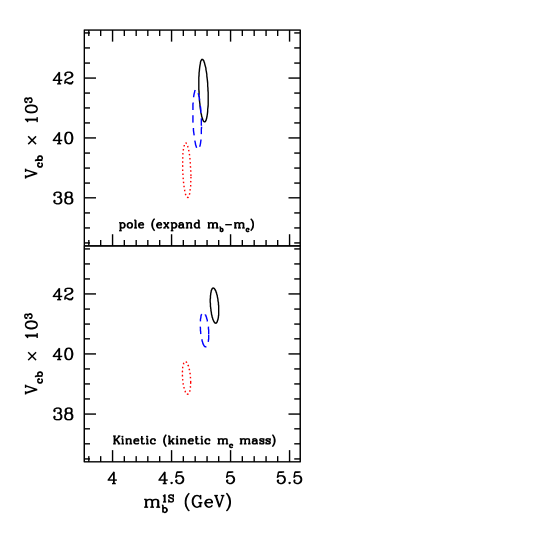
Figure 1: Fit results for $|V_{cb}|$ and $m_{b}$ in the $1S_{\text{EXP}}$, $1S_{\text{NO}}$, $\mbox{kin}_{\text{EXP}}$, $\mbox{kin}_{\text{NO}}$, and $\mbox{kin}_{\text{UG}}$ schemes defined in Eq. (6) and in the traditional pole scheme. The red doted, blue dashed, and black solid ellipses denote the results at tree level, order $\alpha_{s}$, and $\alpha_{s}^{2}\beta_{0}$, respectively, corresponding to $\Delta\chi^{2}=1$.

Scheme	$\sigma^{2}_{\text{theory}}$	$\chi^{2}/\nu$	$|V_{cb}|\times 10^{3}$	$m_{b}^{1S}\,[\mbox{GeV}]$	$m_{b}-m_{c}\,[\mbox{GeV}]$	$\overline{m}_{c}(\overline{m}_{c})\,[\mbox{GeV}]$	$\lambda_{1}\,[\mbox{GeV}^{2}]$
$1S_{\text{EXP}}$	yes	$50.9/86$	$41.4\pm 0.6$	$4.68\pm 0.03$	$3.41\pm 0.01$	$1.07\pm 0.04$	$-0.27\pm 0.04$
$\mbox{kin}_{\text{EXP}}$	yes	$52.6/86$	$41.2\pm 0.6\pm 0.1$	$4.70\pm 0.03\pm 0.03$	$3.40\pm 0.01\pm 0.01$	$1.09\pm 0.03\pm 0.03$	$-0.19\pm 0.04\pm 0.04$
$1S_{\text{EXP}}$	no	$148.4/86$	$41.5\pm 0.3$	$4.69\pm 0.02$	$3.39\pm 0.01$	$1.09\pm 0.02$	$-0.31\pm 0.03$
$\mbox{kin}_{\text{EXP}}$	no	$238.8/86$	$41.1\pm 0.3\pm 0.7$	$4.74\pm 0.01\pm 0.11$	$3.36\pm 0.01\pm 0.04$	$1.15\pm 0.01\pm 0.11$	$-0.33\pm 0.03\pm 0.11$

Table 1: Fit results for $|V_{cb}|$, $m_{b}$, $m_{c}$ and $\lambda_{1}$ in the $1S_{\text{EXP}}$  and $\mbox{kin}_{\text{EXP}}$  schemes. Our fits in the kinetic scheme use $\mu_{\pi}^{2}$, but the result is converted to $\lambda_{1}$ to help comparison. The first two lines are the fit results including our estimates of the theoretical errors, the lower two lines are setting these to zero. The second error for the $\mbox{kin}_{\text{EXP}}$ scheme is the shift due to changing $\mu$ from 1 to 1.5 GeV.

V.3 Constraints on parameters

Even though there are many more observables than there are parameters, the fit does not provide strong constraints on the $1/m_{b}^{3}$ parameters. Thus it is useful to add additional information to ensure that the fit converges to physically sensible values of the nonperturbative parameters. Thus, as in Ref. Bauer:2002sh we add to $\chi^{2}$ the contribution

$$\chi^{2}_{\text{param}}(m_{\chi},M_{\chi})=\cases{0\,,&$|\langle{\cal O}\rangle|\leq m_{\chi}^{3}$\,,\cr\left[|\langle\mathcal{O}\rangle|-m_{\chi}^{3}\right]^{2}/M_{\chi}^{6}\,,&$|\langle{\cal O}\rangle|>m_{\chi}^{3}$\,,\cr}$$ (24)

where $(m_{\chi},M_{\chi})$ are both quantities of order $\Lambda_{\rm QCD}$, and $\langle{\cal O}\rangle$ are the matrix elements of any of the $1/m^{3}$ operators in the fit. This way we do not prejudice $\langle\mathcal{O}\rangle$ to have any particular value in the range $|\langle{\cal O}\rangle|\leq m_{\chi}^{3}$. In the fit we take $M_{\chi}=m_{\chi}=500\,\mbox{MeV}$. We checked in Ref. Bauer:2002sh that the results for $|V_{cb}|$ and $m_{b}$ are insensitive to varying $m_{\chi}$ between 500 MeV and 1 GeV. The data are sufficient to constrain the $1/m_{b}^{3}$ operators in the sense that they can be consistently fit with reasonable values, but they are not determined with any useful precision. The data can be fit without including $\chi^{2}_{\text{param}}$, but then some of the $1/m_{b}^{3}$ parameters are not of natural size, with values of order $0.5~{}\text{GeV}^{3}$. Including $\chi^{2}_{\text{param}}$ gives a fit with reasonable values of the parameters, of order $0.1~{}\text{GeV}^{3}$. The contribution of $\chi^{2}_{\text{param}}$ is rather small, of order $0.1-0.2$, so that $\chi^{2}_{\text{param}}$ does not drive the fit. This shows that there are some very flat directions in parameter space which are stabilized by including $\chi^{2}_{\text{param}}$. We have shown our final results for $V_{cb}$ and $m_{b}$ with and without including $\chi^{2}_{\text{param}}$ in the fit. The final results do not depend significantly on whether or not $\chi^{2}_{\text{param}}$ is included.

Note that the fit performed by the BABAR Collaboration included the half-integer hadronic moments. We have checked that including these moments still leaves some $1/m_{b}^{3}$ parameters with values larger than natural size. We have chosen to not include these moments in the fit since they have large theoretical uncertainties.

Figure 2: Measurements (blue squares: BABAR Aubert:2004te ; Aubert:2004td , green triangles: CLEO Csorna:2004kp ; Mahmood:2004kq , black dots: BELLE Abe:2004ks ; Abe:2004zv ) and fit results for the hadron invariant mass (left) and the lepton energy moments (right) as functions of the lepton energy cut, $E_{\rm cut}$. For the hadron moments $m_{X}^{n}$ denotes $\langle m_{X}^{n}\rangle$, while for the lepton moments BR is branching ratio, M1 is first moment, and M2 and M3 are the second and third central moments, respectively. The red (dark) shaded regions show the fit error, while the yellow (light) shaded regions are our estimates of the theoretical uncertainties from the $A$ terms in Eq. (23). The $A$ term for $\langle m_{X}\rangle$ and $\langle m_{X}^{3}\rangle$ is three times larger than for $\langle m_{X}^{2}\rangle$ and $\langle m_{X}^{4}\rangle$, because of the worse expansion for the non-integer moments.

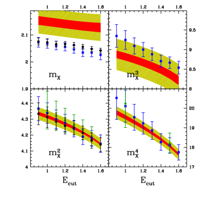
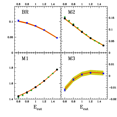
Figure 3: Measurements and fit results for the hadron invariant mass and the lepton energy moments, setting all theory errors to zero in the fit. (See the caption for Fig. 2.) The yellow (light) shaded band gives the estimated theoretical uncertainty, as in Fig 2. It is not included in the fit, but it can help to decide the significance of any differences between theory and experiment.

VI Fit Results and Discussion

The fit result for $|V_{cb}|$ and $m_{b}$ in the five mass schemes defined in Eq. (6) and in the traditional pole scheme are shown in Fig. 1. The fit results are shown at tree level, order $\alpha_{s}$, and order $\alpha_{s}^{2}\beta_{0}$. The kinetic scheme results are obtained using $\mu_{\pi}^{2}$ etc. in the fit, and then converting the results back to $\lambda_{1}$ etc. for easier comparison with the other schemes. One can see that the $1S_{\text{EXP}}$ and $\mbox{kin}_{\text{EXP}}$ schemes have better convergence than the pole scheme. The main fit results in the $1S_{\text{EXP}}$ and $\mbox{kin}_{\text{EXP}}$ scheme are given in Table 1. The quoted $|V_{cb}|$ values include electromagnetic radiative corrections, that reduce $|V_{cb}|$ by $\eta_{\rm QED}=1+(\alpha_{\rm em}/\pi)\ln(m_{W}/\mu)\approx 1.007$. The remarkable agreement between the fit results shows that the main difference in the fits is not which short distance $b$ quark mass is used, but whether $m_{b}-m_{c}$ is or is not expanded in terms of HQET matrix elements.

The uncertainties for the $1S_{\text{EXP}}$ and $\mbox{kin}_{\text{EXP}}$ schemes, which eliminate $m_{c}$, are smaller than for the $1S_{\text{NO}}$ and $\mbox{kin}_{\text{NO}}$ schemes, which use $\overline{m}_{c}(m_{b})$. This is contrary to the claims made in Gambino:2004qm , but is not unexpected, since the former schemes have only one parameter at leading order in $1/m_{b}$, while the latter schemes have two such parameters. While not expanding in $1/m_{c}$ gives slightly larger errors than expanding, the consistency of the central values between the two methods shows that one can use the $1/m_{c}$ expansion for inclusive $B$ decays.

One can clearly see that using the kinetic mass for $m_{c}$ (the $\mbox{kin}_{\text{UG}}$ scheme) does not reduce the uncertainties compared to the $1S_{\text{EXP}}$ and $\mbox{kin}_{\text{EXP}}$ schemes. Also, as is now well known, the pole scheme does not work as well in inclusive calculations as the schemes which use a short distance mass. Thus, in the remainder of this work we will present results in the $1S_{\text{EXP}}$ and in the $\mbox{kin}_{\text{EXP}}$ schemes. We have carried out the fits in 6 additional schemes, including the PS and $\overline{\rm MS}$ schemes. All of the schemes give reasonable fits, but only the PS scheme with $m_{b}-m_{c}$ expanded in HQET gives rise to similarly small uncertainties as $1S_{\text{EXP}}$ and $\mbox{kin}_{\text{EXP}}$.

The charm quark mass enters into the computation, and we can extract the value of $m_{c}$ from our fit. The value of $m_{b}-m_{c}$, which is free of the order $\Lambda_{\rm QCD}$ renormalon ambiguity, is (in the $1S_{\text{EXP}}$ scheme)

$$m_{b}-m_{c}=3.41\pm 0.01~{}\mbox{GeV}\,.$$ (25)

We can convert this result to the $\overline{\rm MS}$ mass of the charm quark,

$$\overline{m}_{c}(\overline{m}_{c}) = 0.90\pm 0.04~{}\text{GeV}\,,$$

$$\overline{m}_{c}(\overline{m}_{c}) = 1.07\pm 0.04~{}\text{GeV}\,,$$ (26)

where the two results depend on whether the perturbative conversion factor is reexpanded or not. The reason for the large difference between the two results is that perturbative corrections are large at the scale $\overline{m}_{c}$. Taking the average of the two $m_{c}$ values, and adding half the difference between them as an additional error gives

$$\overline{m}_{c}(\overline{m}_{c})=0.99\pm 0.1~{}\text{GeV}\,.$$ (27)

The difference between the $m_{c}$ values is a nice illustration that one should avoid using perturbation theory at a low scale, if at all possible. The $\mbox{kin}_{\text{UG}}$ scheme uses perturbation theory at a scale below $m_{c}$, and suffers from the same problem.

Next, we compare how well the theory can reproduce the experimental measurements, focusing on the cut dependence of individual moments. The results for the hadronic moments and the leptonic moments are shown in Fig. 2 in the $1S_{\text{EXP}}$ scheme. (The DELPHI and CDF results are included in the fits, but are not shown, as they correspond to $E_{\rm cut}=0$.). The red (dark) shaded band is the uncertainty due to the errors on the fit parameter. The width of the yellow (light) shaded band is the theoretical uncertainty due to higher order nonperturbative effects not included in the computation [the $A$ term in Eq. (23)]. Within the uncertainties, the OPE predictions for all these moments agree well with the data. As we explained before, the moments $\langle m_{X}\rangle$ and $\langle m_{X}^{3}\rangle$ were not included in the fit. The yellow bands shown for $\langle m_{X}\rangle$ and $\langle m_{X}^{3}\rangle$ use $A=0.003$ as an estimate of the uncertainty, a factor of three larger than for the integer moments, because of the worse theoretical expansion discussed in Sec. III.3.

The agreement between the theory and experiment for the third lepton moment is better than our estimate of the theoretical uncertainty. This might be an indication that we overestimate the theoretical uncertainty for this moment.

The $\chi^{2}$ for the fit shows that the theory provides an excellent description of the data. In the $1S_{\text{EXP}}$ scheme, we get $\chi^{2}=50.9$ for $\nu=86$ degrees of freedom, so $\chi^{2}/\nu=0.59$. The standard deviation for $\chi^{2}/\nu$ is $\sqrt{2/\nu}=0.17$, so that $\chi^{2}/\nu=0.59$ is about two standard deviations below the mean value of 1.01. This is some evidence that the theoretical errors have been overestimated. To study the effect of the theoretical uncertainties, we also perform fits with all theoretical uncertainties set to zero. This fit gives $\chi^{2}=148.4$ for the $1S_{\text{EXP}}$ scheme, and $\chi^{2}=238.8$ for the $\mbox{kin}_{\text{EXP}}$ scheme. The resulting fits still agree well with the experimental data, as can be seen from Fig. 3. The fit results with no theory error are given in the lower half of Table 1. The values $\chi^{2}/\nu=1.72$ for the $1S_{\text{EXP}}$ scheme and $\chi^{2}/\nu=2.72$ for the $\mbox{kin}_{\text{EXP}}$ scheme are significantly greater than one, which is some evidence that there are higher order theoretical effects which have not been included.

The calculations in the $\mbox{kin}_{\text{UG}}$ scheme Gambino:2004qm were used by the BABAR Collaboration Aubert:2004aw , to perform a fit to its own data. While we agree with the results of Ref. Gambino:2004qm for the lepton energy moments, we are unable to reproduce their results for the hadronic invariant mass moments. One should also note that Ref. Gambino:2004qm (i) uses $\alpha_{s}=0.22$ for the lepton moments, and $\alpha_{s}=0.3$ for the hadron moments (ii) includes the $\alpha_{s}^{2}\beta_{0}$ corrections (which are known for both the lepton and integer hadron moments) only in the lepton moments, but not in the hadron moments.

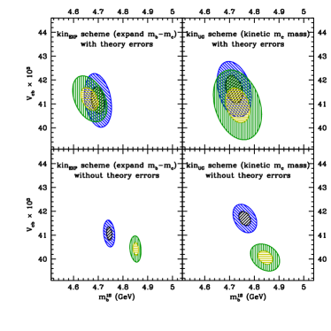
Figure 4: Fit results for $|V_{cb}|$ and $m_{b}$ in the $\mbox{kin}_{\text{EXP}}$ and $\mbox{kin}_{\text{UG}}$ schemes using $\mu_{b}=1$ GeV (blue and black) and using $\mu_{b}=1.5\,$ GeV (green and yellow). $\mu_{c}$ for the $\mbox{kin}_{\text{UG}}$ scheme has been kept fixed at 1 GeV. The regions correspond to $\Delta\chi^{2}=1$ (black and yellow) and 4 (blue and green). The upper plots includes theory errors in the fit, and the lower plot does not.

The $\mbox{kin}_{\text{EXP}}$ and $\mbox{kin}_{\text{NO}}$ schemes depend on a choice for $\mu_{b}$. In the $\mbox{kin}_{\text{UG}}$ scheme there is an additional dependence on $\mu_{c}$, and there is no reason why the theoretical predictions should be expanded using $m_{b}^{\rm kin}(\mu_{b})$ and $m_{c}^{\rm kin}(\mu_{c})$ defined at the same scale ($\mu_{b}=\mu_{c}$), since all that is required is that each $\mu$ should be small, so one has to choose both $\mu_{b}$ and $\mu_{c}$. To illustrate the sensitivity to the choice of $\mu_{b,c}$ we show a fit in Fig. 4 varying $\mu_{b}$ from 1 to 1.5 GeV keeping $\mu_{c}=1\,$GeV fixed. Clearly there is significant dependence in the kinetic schemes with respect to changes in $\mu$, and this should be included as an additional uncertainty for that scheme. We have included this scale uncertainty in Table 1. The kinetic schemes use perturbation theory at a low scale $\mu_{b,c}$, and so are sensitive to precisely how these corrections are included, as was the case for $\overline{m}_{c}(\overline{m}_{c})$. The PS scheme is much less sensitive to the value of $\mu$. In Fig. 5, we show the variation with $\mu$ in the PS scheme. Note that one advantage of the $1S$ scheme is that it does not depend on any factorization scale parameter $\mu$.

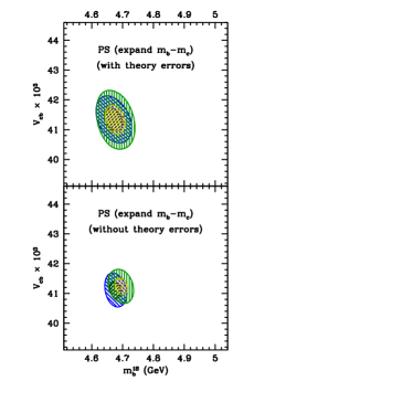
Figure 5: Fit results for $|V_{cb}|$ and $m_{b}$ in the PS scheme using $\mu=2\,$ GeV (blue and black) and using $\mu=1.5\,$ GeV (green and yellow) The regions correspond to $\Delta\chi^{2}=1$ (black and yellow) and 4 (blue and green). The upper plots includes theory errors in the fit, and the lower plot does not.

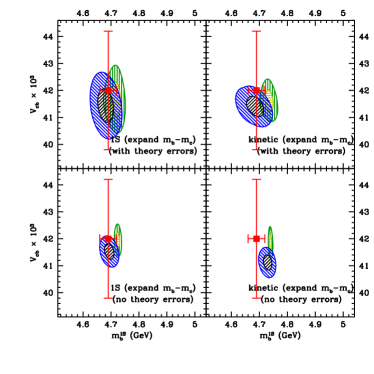
Figure 6: Fit results for $|V_{cb}|$ and $m_{b}$ in the $1S_{\text{EXP}}$ and $\mbox{kin}_{\text{EXP}}$ schemes. The upper plots include our estimate of the theoretical errors, the lower ones set them to zero. The black and blue regions are the fit results ($\Delta\chi^{2}=1,4$), and the yellow and green regions are the fit results ($\Delta\chi^{2}=1,4$) omitting $\chi^{2}_{\text{param}}$ in Eq. (24). We have also shown a red point given by combining Hoang’s determination of $m_{b}^{1S}$ and the PDG 2004 value of $|V_{cb}|$ from exclusive decays.

$\begin{array}[]{c|c|c|c|c|c}\hline\cr\hline\cr E_{\text{cut}}\ (\text{GeV})&0.6&0.8&1.0&1.2&1.4\\ \hline\cr\displaystyle{{\cal B}(B\to X_{c}\ell\bar{\nu})\over{\cal B}(B\to X_{c}\ell\bar{\nu},E_{\text{cut}})}={R_{0}(0,0)\over R_{0}(E_{\text{cut}},0)}&1.0523\pm 0.0001&1.1216\pm 0.0003&1.246\pm 0.001&1.466\pm 0.001&1.880\pm 0.003\\ \hline\cr\hline\cr\end{array}$

Table 2: The ratio of the semileptonic branching ratio ${\cal B}(B\to X_{c}\ell\bar{\nu})$ to the semileptonic branching ratio with a lepton energy cut $E_{\text{cut}}$ obtained using the $1S_{\text{EXP}}$ scheme, including theoretical uncertainties.

Reference Gambino:2004qm quotes smaller theoretical errors than the estimates used here, as can be seen from the plots in Ref. Aubert:2004aw . We do not believe that this optimistic estimate of the theoretical uncertainty is justified.

Figure 6 shows the results for $|V_{cb}|$ and $m_{b}$ in the $1S_{\text{EXP}}$ and $\mbox{kin}_{\text{EXP}}$ schemes with and without including our estimate of the theoretical uncertainties. This plot also shows for comparison $m_{b}=4.69\pm 0.03\,\mbox{GeV}$ extracted by Hoang hoang from sum rules Beneke ; Voloshin that fit to the $\bar{B}B$ system near threshold, and the PDG 2004 value pdg $|V_{cb}|=\left(42.0\pm 1.1\pm 1.8\right)\times 10^{-3}$ from exclusive decays. Hoang’s determination of $m_{b}^{1S}$ is independent of the current determination, and the agreement is remarkable. The PDG 2004 value for $|V_{cb}|$ from exclusive decays is also independent of our determination from inclusive decays.

In summary, we find the following fit results:

$$|V_{cb}| = \left(41.4\pm 0.6\pm 0.1_{\tau_{B}}\right)\times 10^{-3},$$

$$m_{b}^{1S} = (4.68\pm 0.03)\,\text{GeV},$$ (28)

from the $1S_{\text{EXP}}$ fit including theory errors, where the first error is the uncertainty from the fit, and the second error (for $|V_{cb}|$) is due to the uncertainty in the average $B$ lifetime. From the $1S_{\text{EXP}}$ fit with no theory errors, and using the PDG method of scaling the uncertainties so that $\chi^{2}/\nu$ is unity, we obtain

$$|V_{cb}| = \left(41.5\pm 0.4\pm 0.1_{\tau_{B}}\right)\times 10^{-3},$$

$$m_{b}^{1S} = (4.69\pm 0.02)\,\text{GeV}.$$ (29)

The increase in $|V_{cb}|$ compared to Ref. Bauer:2002sh is largely due to an increase in the experimental values for the semileptonic $B$ decay rate since two years ago.

The $1S_{\text{EXP}}$ fit (including theoretical uncertainties) also gives

$${\Gamma(B\to X_{c}\ell\bar{\nu})\over|V_{cb}|^{2}\,\eta_{\text{QED}}^{2}}=(2.49\pm 0.02)\times 10^{-11}\ \text{GeV}.$$ (30)

The ratio of the semileptonic branching ratio with no energy cut to that with an energy cut is given Table 2. The semileptonic branching ratio obtained from the fit (including theoretical uncertainties) is ${\cal B}(B\to X_{c}\ell\bar{\nu})=0.105\pm 0.003$. Note that this number depends on the PDG 2004 value (corrected for $B\to X_{u}$ contamination, see Eq. (9)) of $0.105\pm 0.003$, and the BABAR branching ratio measurements with an energy cut, which give a higher value of $0.107\pm 0.002$, when converted to the branching ratio using Table 2.

Another useful quantity is the $C$ parameter, needed for the $B\to X_{s}\gamma$ rate misiak , which is defined to be

$$C={\Gamma(B\to X_{c}\ell\bar{\nu})\over|V_{cb}|^{2}}\,{|V_{ub}|^{2}\over\Gamma(B\to X_{u}\ell\bar{\nu})}=0.58\pm 0.01\,.$$ (31)

The value of $C$ depends on the (unknown) matrix element of four-quark operators, which enter the $B\to X_{u}\ell\bar{\nu}$ rate at order $1/m_{b}^{3}$ (but not $B\to X_{c}\ell\bar{\nu}$). These absorb a logarithmic divergence in the $1/m_{b}^{3}$ corrections to the $B\to X_{c}\ell\bar{\nu}$ rate in the formal limit $m_{c}\to 0$. (For $m_{c}\gg\Lambda_{\rm QCD}$, four-quark operators only enter the $B\to X_{c}\ell\bar{\nu}$ rate at order $\alpha_{s}$.) The four-quark operator matrix element gives an uncertainty in addition to that in Eq. (31). An estimate of the four-quark operators’ contribution is obtained by replacing the formally divergent term in the $B\to X_{u}\ell\bar{\nu}$ rate, $8(\rho_{1}/m_{b}^{3})\ln(m_{u}^{2}/m_{b}^{2})$ GK by $8(\Lambda_{\rm QCD}/m_{b})^{3}\sim 0.01$ BB .

The above fits give a robust value for $|V_{cb}|$ and $m_{b}$. However, we recommend using the error estimate with caution. As we have pointed out, the fit seems to indicate that the unknown higher order corrections are smaller than our theoretical estimate of $0.1\%$, so that one can use Eq. (VI). A theoretical uncertainty less than $0.1\%$ is very small for a hadronic quantity at the relatively low scale of around 5 GeV. It is interesting that the current fit shows that the theoretical uncertainties in inclusive $B$ decay shape variables are so small. If this is confirmed by further comparisons between theory and experiment, the uncertainty in $V_{cb}$ can be reduced still further.