Astrophysical Bounds on
Planck Suppressed Lorentz Violation

This article reviews many of the observational constraints on Lorentz symmetry violation (LV). We first describe the GZK cutoff and other phenomena that are sensitive to LV. After a brief historical sketch of research on LV, we discuss the effective field theory description of LV and related questions of principle, technical results, and observational constraints. We focus on constraints from high energy astrophysics on mass dimension five operators that contribute to LV electron and photon dispersion relations at order $E/M_{\rm Planck}$. We also briefly discuss constraints on renormalizable operators, and review the current and future contraints on LV at order $(E/M_{\rm Planck})^{2}$.

1 Windows on quantum gravity?

In most fields of physics it goes without saying that observation and prediction play a central role, but unfortunately quantum gravity (QG) has so far not fit that mold. Many intriguing and ingenious ideas have been explored, but it seems safe to say that without both observing phenomena that depend on QG, and extracting reliable predictions from candidate theories that can be compared with observations, the goal of a theory capable of incorporating quantum mechanics and general relativity will remain unattainable.

Besides the classical limit, there is one observed phenomenon for which quantum gravity makes a prediction that has received encouraging support: the spectrum of primordial cosmological perturbations. The quantized longitudinal linearized gravitational mode, albeit slave to the inflaton and not a dynamically independent degree of freedom, plays an essential role in this story Mukhanov:1990me .

What other types of phenomena might be characteristic of a quantum gravity theory? Motivated by tentative theories, partial calculations, intimations of symmetry violation, hunches, philosophy, etc, some of the proposed ideas are: loss of quantum coherence or state collapse, QG imprint on initial cosmological perturbations, scalar moduli or other new fields, extra dimensions and low-scale QG, deviations from Newton’s law, black holes produced in colliders, violation of global internal symmetries, and violation of spacetime symmetries. It is this last item, more specifically the possibility of Lorentz violation (LV), that is the focus of these lecture notes.

From the observational point of view, developments are encouraging a new look at the possibility of LV. Increased detector size, space-borne instruments, technological improvement, and technique refinement are permitting observations to probe higher energies, weaker interactions, lower fluxes, lower temperatures, shorter time resolution, and longer distances. It comes as a welcome surprise that the day of true quantum gravity observations may not be so far off Dawn .

2 Lorentz violation

Lorentz symmetry is linked to a scale-free nature of spacetime: unbounded boosts expose ultra-short distances, and yet nothing changes. However, suggestions for Lorentz violation have come from: the need to cut off UV divergences of quantum field theory and of black hole entropy, tentative calculations in various QG scenarios (e.g. semiclassical spin-network calculations in Loop QG, string theory tensor VEVs, non-commutative geometry, some brane-world backgrounds), and the possibly missing GZK cutoff GZK on ultra-high energy (UHE) cosmic rays.

The GZK question has generated a lot of interest, and is currently the only observational phenomenon thought to indicate a possible violation of Lorentz symmetry. As an invitation to the subject, we discuss it in this section, before embarking on the rest of the lectures. We also give a list of possible LV phenomena, and a brief historical overview of the subject.

2.1 The GZK cut-off

In collisions of ultra high energy protons with cosmic microwave background (CMB) photons there can be sufficient energy in the center of mass frame to create a pion, leading to the the reaction

$$p+\gamma_{\rm CMB}\rightarrow p+\pi^{0}.$$ (1)

The threshold occurs when the invariant magnitude of the total four momentum is the sum of the proton and pion mass, since at threshold these particles are both at rest in the zero-momentum frame. That is, it occurs when $(p_{p}+p_{\gamma})^{2}=(m_{p}+m_{\pi})^{2}$, or $p_{p}\cdot p_{\gamma}=m_{p}m_{\pi}+\frac{1}{2}m_{\pi}^{2}$, where $p_{p,\gamma}$ are the proton and photon 4-momenta, and $m_{p,\pi}$ are the proton and pion mass. Since $E_{p}\gg m_{p}$, and $m_{\pi}\ll 2m_{p}$, this yields the proton energy threshold

$$E_{GZK}\simeq\frac{m_{p}m_{\pi}}{2E_{\gamma}}\simeq 3\times 10^{20}{\rm eV}\times\left(\frac{2.7{\rm K}}{E_{\gamma}}\right)$$ (2)

To get a definite number we have put $E_{\gamma}$ equal to the energy of a photon at the CMB temperature, 2.7K, but of course the CMB contains photons of higher energy,

This process degrades the initial proton energy with an attenuation length of about 50 Mpc. Since plausible astrophysical sources for UHE particles are located at distances larger than 50 Mpc, one expects a cutoff in the cosmic ray proton energy spectrum, which occurs at around $5\times 10^{19}$ eV, depending on the distribution of sources Stecker:2003wm .

One of the experiments measuring the UHE cosmic ray spectrum, the AGASA experiment, has not seen the cutoff. An analysis DeMarco:2003ig from January 2003 concluded that the cutoff was absent at the 2.5 sigma level, while another experiment, HiRes, is consistent with the cutoff but at a lower confidence level. (For a brief review of the data see Stecker:2003wm .) The question should be answered in the near future by the AUGER observatory, a combined array of 1600 water Čerenkov detectors and 24 telescopic air flouresence detectors under construction on the Argentine pampas Auger . The new observatory will see an event rate one hundred times higher, with better systematics.

Many ideas have been put forward to explain the possible absence of the GZK cutoff Stecker:2003wm . For example the cosmic rays might originate closer, in some unexpected way, by astrophysical acceleration or by decay of ultra-heavy exotic particles, or they may be produced by collisions with ultra high energy cosmic neutrinos. Virtually all of these explanations have problems.

In this context, it is intriguing to consider that with even a tiny amount of Lorentz violation the energy threshold for the GZK reaction could be affected. According to equation (2) the Lorentz invariant threshold is proportional to the proton mass. Thus any LV term added to the proton dispersion relation $E^{2}={\bf p}^{2}+m^{2}$ will modify the threshold if it is comparable to or greater than $m_{p}^{2}$ at around the energy $E_{GZK}$. Modifying the proton and pion dispersion relations, the threshold can be lowered, raised, or removed entirely, or even an upper threshold where the reaction cuts off could be introduced (see e.g. Jacobson:2002hd and references therein).

For example, the LV term considered by Coleman and Glashow CG-GZK was of the form $\eta{\bf p}^{2}$, assumed given in a reference frame close to that of the earth, which is natural since we are close to being at rest in the universal rest frame. This would affect the GZK threshold as long as $\eta>(m_{p}/E_{GZK})^{2}\sim 10^{-22}$. Even LV suppressed by two powers of the Planck mass $M$ would affect the threshold: a term of the form ${\bf p}^{4}/M^{2}$ is comparable to $m_{p}^{2}$ when the proton energy is $(m_{p}M)^{1/2}\simeq 3\times 10^{18}$ eV, which is two orders of magnitude below the highest energy cosmic rays. Thus a missing GZK cutoff could be explained by Planck double-suppressed LV. Conversely, observational confirmation of the GZK cutoff can severely constrain such LV.

2.2 Possible LV phenomena

Trans-GZK cosmic rays are not the only window of opportunity we have to detect or constrain Lorentz violation induced by QG effects. In fact, many phenomena accessible to current observations/experiments are sensitive to possible violations of Lorentz invariance. A partial list is

• sidereal variation of LV couplings as the lab moves with respect to a preferred frame or directions

• long baseline dispersion and vacuum birefringence (e.g. of signals from gamma ray bursts, active galactic nuclei, pulsars, galaxies)

• new reaction thresholds (e.g. photon decay, vacuum Čerenkov effect)

• shifted thresholds (e.g. photon annihilation from blazars, GZK reaction)

• maximum velocity (e.g. synchrotron peak from supernova remnants)

• dynamical effects of LV background fields (e.g. gravitational coupling and additional wave modes)

2.3 A brief history of some LV research

We conclude this section with a brief historical overview mentioning some of the more influential papers, but by no means complete.

Suggestions of possible LV in particle physics go back at least to the 1960’s, when a number of authors wrote on that idea Dirac . The possibility of LV in a metric theory of gravity was explored beginning at least as early as the 1970’s LVmetr . Such theoretical ideas were pursued in the ’70’s and ’80’s notably by Nielsen and several other authors on the particle theory side 7080theory , and by Gasperini Gasp on the gravity side. A number of observational limits were obtained during this period HauganAndWill .

Towards the end of the 80’s Kostelecky and Samuel KS presented evidence for possible spontaneous LV in string theory, and motivated by this explored LV effects in gravitation. The role of Lorentz invariance in the “trans-Planckian puzzle” of black hole redshifts and the Hawking effect was emphasized in the early 90’s TedUltra . This led to study of the Hawking effect for quantum fields with LV dispersion relations commenced by Unruh Unruh and followed up by others. Early in the third millenium this line of research led to work on the related question of the possible imprint of trans-Planckian frequencies on the primordial fluctuation spectrum BM . Meanwhile the consequences of LV for particle physics were being explored using LV dispersion relations e.g. by Gonzalez-Mestres GM .

Four developments in the late nineties seem to have stimulated a surge of interest in LV research. One was a systematic extension of the standard model of particle physics incorporating all possible LV in the renormalizable sector, developed by Colladay and Kostelecký CK . That provided a framework for computing the observable consequences for any experiment and led to much experimental work setting limits on the LV parameters in the lagrangian AKbook . On the observational side, the AGASA experiment reported events beyond the GZK cutoff Takeda:1998ps . Coleman and Glashow then suggested the possibility that LV was the culprit in the possibly missing GZK cutoff CG-GZK , and explored many other high energy consequences of renormalizable, isotropic LV leading to different limiting speeds for different particles CGlong . In the fourth development, it was pointed out by Amelino-Camelia et al GAC-Nat that the sharp high energy signals of gamma ray bursts could reveal LV photon dispersion suppressed by one power of energy over the mass $M\sim 10^{-3}M_{\rm P}$, tantalizingly close to the Planck mass.

Together with the improvements in observational reach mentioned earlier, these developments attracted the attention of a large number of researchers to the subject. Shortly after Ref. GAC-Nat appeared, Gambini and Pullin GP argued that semiclassical loop quantum gravity suggests just such LV. Some later work supported this notion, but the issue continues to be debated KP ; Alfaro:2004ur . In any case, the dynamical aspect of the theory is not under enough control at this time to make any definitive statements concerning LV.

A very strong constraint on photon birefringence was obtained by Gleiser and Kozameh GK using UV light from distant galaxies. If the recent reportCB03 of polarized gamma rays from a GRB turns out to be correct despite the concerns of Refs. RF03 , this constraint will be further strengthened dramatically JLMS ; Mitro . Further stimulus came from the suggestion PM that an LV threshold shift might explain the apparent under-absorption on the cosmic IR background of TeV gamma rays from the blazar Mkn501, however it is now believed by many that this anomaly goes away when a corrected IR background is used Kono .

The extension of the effective field theory framework to include LV dimension 5 operators was introduced by Myers and Pospelov MP , and used to strengthen prior constraints. Also this framework was used to deduce a very strong constraint Crab on the possibility of a maximum electron speed less than the speed of light from observations of synchrotron radiation from the Crab Nebula.

3 Theoretical framework for LV

Various different theoretical approaches to LV have been taken to pursue the ideas summarized above. Some researchers restrict attention to LV described in the framework of effective field theory (EFT), while others allow for effects not describable in this way, such as those that might be due to stochastic fluctuations of a “space-time foam”. Some restrict to rotationally invariant LV, while others consider also rotational symmetry breaking. Both true LV as well as “deformed” Lorentz symmetry (in the context of so-called “doubly special relativity”DSR ) have been pursued. Another difference in approaches is whether one allows for distinct LV parameters for different particle types, or proposes a more universal form of LV.

The rest of this article will focus on just one of these approaches, namely LV describable by standard EFT, assuming rotational invariance, and allowing distinct LV parameters for different particles. In exploring the possible phenomenology of new physics, it seems useful to retain enough standard physics so that clear predictions can be made, and so that the possibilities are narrow enough to be meaningfully constrained.

This approach is not universally favored. For example a sharp critique appears in GAC-crit . Therefore we think it is important to spell out the motivation for the choices we have made. First, while of course it may be that EFT is not adequate for describing the leading quantum gravity phenomenology effects, it has proven itself very effective and flexible in the past. It produces local energy and momentum conservation laws, and seems to require for its validity just locality and local spacetime translation invariance above some length scale. It describes the standard model and general relativity (which are presumably not fundamental theories), a myriad of condensed matter systems at appropriate length and energy scales, and even string theory (as perhaps most impressively verified in the calculations of black hole entropy and Hawking radiation rates). It is true that, e.g., non-commutative geometry (NCG) seems to lead to EFT with problematic IR/UV mixing, however this more likely indicates a physically unacceptable feature of such NCG rather than a physical limitation of EFT.

The assumption of rotational invariance is motivated by the idea that LV may arise in QG from the presence of a short distance cutoff. This suggests a breaking of boost invariance, with a preferred rest frame, but not necessarily rotational invariance. Since a constraint on pure boost violation is, barring a conspiracy, also a constraint on boost plus rotation violation, it is sensible to simplify with the assumption of rotation invariance at this stage. The preferred frame is assumed to coincide with the rest frame of the CMB.

Finally why do we choose to complicate matters by allowing for different LV parameters for different particles? First, EFT for first order Planck suppressed LV (see section 3.2) requires this for different polarizations or spin states, so it is unavoidable in that sense. Second, we see no reason a priori to expect these parameters to coincide. The term “equivalence principle” has been used to motivate the equality of the parameters. However, in the presence of LV dispersion relations, free particles with different masses travel on different trajectories even if they have the same LV parameters Fischbach:wq ; Jacobson:2002hd . Moreover, different particles would presumably interact differently with the spacetime microstructure since they interact differently with themselves and with each other. An example of this occurs in the braneworld model discussed in Ref. Burgess , and an extreme version occurs in the proposal of Ref. emn in which only certain particles feel the spacetime foam effects. (Note however that in this proposal the LV parameters fluctuate even for a given kind of particle, so EFT would not be a valid description.)

3.1 Deformed dispersion relations

A simple approach to a phenomenological description of LV is via deformed dispersion relations. If rotation invariance and integer powers of momentum are assumed in the expansion of $E^{2}({\bf p})$, the dispersion relation for a given particle type can be written as

$$E^{2}=p^{2}+m^{2}+\Delta(p),$$ (3)

where $p$ is hereafter the magnitude of the three-momentum, and

$$\Delta(p)=\tilde{\eta}_{1}p^{1}+\tilde{\eta}_{2}p^{2}+\tilde{\eta}_{3}p^{3}+\tilde{\eta}_{4}p^{4}+\cdots$$ (4)

Since they are not Lorentz invariant, it is necessary to specify the frame in which these relations are given, namely the CMB frame.

Let us introduce two mass scales, $M=10^{19}\,{\rm GeV}\approx M_{\rm Planck}$, the putative scale of quantum gravity, and $\mu$, a particle physics mass scale. To keep mass dimensions explicit we factor out possibly appropriate powers of these scales, defining the dimensionful $\tilde{\eta}$’s in terms of corresponding dimensionless parameters. It might seem natural that the $p^{n}$ term with $n\geq 3$ be suppressed by $1/M^{n-2}$, and indeed this has been assumed in most work. But following this pattern one would expect the $n=2$ term to be unsuppressed and the $n=1$ term to be even more important. Since any LV at low energies must be small, such a pattern is untenable. Thus either there is a symmetry or some other mechanism protecting the lower dimension oprators from large LV, or the suppression of the higher dimension operators is greater than $1/M^{n-2}$. This is an important issue to which we return in section 3.3.

For the moment we simply follow the observational lead and insert at least one inverse power of $M$ in each term, viz.

$$\tilde{\eta}_{1}=\eta_{1}\frac{\mu^{2}}{M},\qquad\tilde{\eta}_{2}=\eta_{2}\frac{\mu}{M},\qquad\tilde{\eta}_{3}=\eta_{3}\frac{1}{M},\qquad\tilde{\eta}_{4}=\eta_{4}\frac{1}{M^{2}}.$$ (5)

In characterizing the strength of a constraint we refer to the $\eta_{n}$ without the tilde, so we are comparing to what might be expected from Planck-suppressed LV. We allow the LV parameters $\eta_{i}$ to depend on the particle type, and indeed it turns out that they must sometimes be different but related in certain ways for photon polarization states, and for particle and antiparticle states, if the framework of effective field theory is adopted. In an even more general setting, Lehnert Leh studied theoretical constraints on this type of LV and deduced the necessity of some of these parameter relations.

The deformed dispersion relations are introduced for elementary particles only; those for macroscopic objects are then inferred by addition. For example, if $N$ particles with momentum $\bf p$ and mass $m$ are combined, the total energy, momentum and mass are $E_{\rm tot}=NE(p)$, ${\bf p}_{\rm tot}=N{\bf p}$, and $m_{\rm tot}=Nm$, so that $E_{\rm tot}^{2}=p_{\rm tot}^{2}+m_{\rm tot}^{2}+N^{2}\Delta(p)$. Although the Lorentz violating term can be large in some fixed units, its ratio with the mass and momentum squared terms in the dispersion relation is the same as for the individual particles. Hence, there is no observational conflict with standard dispersion relations for macroscopic objects.

This general framework allows for superluminal propagation, and spacelike 4-momentum relative to a fixed background metric. It has been argued KL that this leads to problems with causality and stability. In the setting of a LV theory with a single preferred frame, however, we do not share this opinion. As long as the physics is guaranteed to be causal and the states all have positive energy in the preferred frame, we cannot see any room for such problems to arise.

3.2 Effective field theory and LV

The standard model extension (SME) of Colladay and Kostelecký CK consists of the standard model of particle physics plus all Lorentz violating renormalizable operators (i.e. of mass dimension $\leq 4$) that can be written without changing the field content or violating the gauge symmetry. For illustration, the leading order terms in the QED sector are the dimension three terms

$$-b_{a}\bar{\psi}\gamma_{5}\gamma^{a}\psi-\frac{1}{2}H_{ab}\bar{\psi}\sigma^{ab}\psi$$ (6)

and the dimension four terms

$$-\frac{1}{4}k^{abcd}F_{ab}F_{cd}+\frac{i}{2}\bar{\psi}(c_{ab}+d_{ab}\gamma_{5})\gamma^{a}\stackrel{{\scriptstyle\leftrightarrow}}{{D}}\!\!{}^{b}\psi,$$ (7)

where the dimension one coefficients $b_{a}$, $H_{ab}$ and dimensionless $k^{abcd}$, $c_{ab}$, and $d_{ab}$ are constant tensors characterizing the LV. If we assume rotational invariance then these must all be constructed from a given unit timelike vector $u^{a}$ and the Minkowski metric $\eta_{ab}$, hence $b_{a}\propto u_{a}$, $H_{ab}=0$, $k^{abcd}\propto u^{[a}\eta^{b][c}u^{d]}$, $c_{ab}\propto u_{a}u_{b}$, and $d_{ab}\propto u_{a}u_{b}$. Such LV is thus characterized by just four numbers.

The study of Lorentz violating EFT in the higher mass dimension sector was initiated by Myers and Pospelov MP . They classified all LV dimension five operators that can be added to the QED Lagrangian and are quadratic in the same fields, rotation invariant, gauge invariant, not reducible to a combination of lower and/or higher dimension operators using the field equations, and contribute $p^{3}$ terms to the dispersion relation. Just three operators arise:

$$-\frac{\xi}{2M}u^{m}F_{ma}(u\cdot\partial)(u_{n}\tilde{F}^{na})+\frac{1}{M}u^{m}\bar{\psi}\gamma_{m}(\zeta_{1}+\zeta_{2}\gamma_{5})(u\cdot\partial)^{2}\psi$$ (8)

where $\tilde{F}$ denotes the dual of $F$, and $\xi,\zeta_{1,2}$ are dimensionless parameters. The sign of the $\xi$ term in (8) is opposite to that in MP , and is chosen so that positive helicity photons have $+\xi$ for a dispersion coefficient (see below). All of these terms violate CPT symmetry as well as Lorentz invariance. Thus if CPT were preserved, these LV operators would be forbidden.

In the limit of high energy $E\gg m$, the photon and electron dispersion relations following from QED with the above terms are MP

$$\omega_{\pm}^{2} = k^{2}\pm\frac{\xi}{M}k^{3}$$ (9)

$$E_{\pm}^{2} = p^{2}+m^{2}+\frac{2(\zeta_{1}\pm\zeta_{2})}{M}p^{3}.$$ (10)

The photon subscripts $\pm$ refer to helicity, i.e. right and left circular polarization, which it turns out necessarily have opposite LV parameters. The electron subscripts $\pm$ refer to the helicity, which can be shown to be a good quantum number in the presence of these LV terms JLMS . Moreover, if we write $\eta_{\pm}=2(\zeta_{1}\pm\zeta_{2})$ for the LV parameters of the two electron helicities, those for positrons are given JLMS by

$$\eta^{\rm positron}_{\pm}=-\eta^{\rm electron}_{\mp}.$$ (11)

If $\eta_{1}=0$, then the two helicities have opposite LV paprameters, $\eta_{+}=-\eta_{-}$, so electron and positron have the same LV parameters. If instead $\eta_{2}=0$, then the $\eta_{+}=\eta_{-}$, so electron and positron have opposite LV parameters.

3.3 Naturalness of small LV at low energy?

As discussed above in subsection 3.1, if LV operators of dimension $n>4$ are suppressed, as we have imagined, by $1/M^{n-2}$, LV would feed down to the lower dimension operators and be strong at low energies CGlong ; MP ; PerezSudarsky ; Collins , unless there is a symmetry or some other mechanism that protects the lower dimension operators from strong LV. What symmetry (other than Lorentz invariance, of course!) could that possibly be?

In the Euclidean context, a discrete subgroup of the Euclidean rotation group suffices to protect the operators of dimension four and less from violation of rotation symmetry. For example Hyper , consider the “kinetic” term in the EFT for a scalar field with hypercubic symmetry, $M^{\mu\nu}\partial_{\mu}\phi\partial_{\nu}\phi$. The only tensor $M^{\mu\nu}$ with hypercubic symmetry is proportional to the Kronecker delta $\delta^{\mu\nu}$, so full rotational invariance is an “accidental” symmetry of the kinetic operator.

If one tries to mimic this construction on a Minkowski lattice admitting a discrete subgroup of the Lorentz group, one faces the problem that each point has an infinite number of neighbors related by the Lorentz boosts. For the action to share the discrete symmetry each point would have to appear in infinitely many terms of the discrete action, presumably rendering the equations of motion meaningless.

Another symmetry that could do the trick is three dimensional rotational symmetry together with a symmetry between different particle types. For example, rotational symmetry would imply that the kinetic term for a scalar field takes the form $(\partial_{t}\phi)^{2}-c^{2}(\nabla\phi)^{2}$, for some constant $c$. Then, for multiple scalar fields, a symmetry relating the fields would imply that the constant $c$ is the same for all, hence the kinetic term would be Lorentz invariant with $c$ playing the role of the speed of light. Unfortunately this mechanism does not work in nature, since there is no symmetry relating all the physical fields.

Perhaps under some conditions a partial symmetry could be adequate, e.g. grand unified gauge and/or super symmetry. In fact, a recent analysis of Nibbelink and Pospelov Nibbelink:2004za presents evidence that supersymmetry (SUSY) together with gauge symmetry might indeed play this role. SUSY here refers to the symmetry algebra that is a kind of square root of the spacetime translation group. The nature of this square root depends upon the Minkowski metric, so is tied to the Lorentz group, but it does not require Lorentz symmetry. It is shown in Ref. Nibbelink:2004za , using the superfield formalism, that the SUSY preserving LV operators that can be added to the SUSY Standard Model first appear at dimension five. Moreover, these operators do not contribute $O(p^{3})$ terms to the particle dispersion relations. Of course SUSY is broken in the real world, but the suppression in the SUSY theory may mean that the low dimension LV terms allowed in the presence of soft SUSY breaking are suppressed enough to be compatible with observation. On the other hand, it might also mean that they are so suppressed as to lie beyond the scope of observation.

At this stage we assume the existence of some realization of the Lorentz symmetry breaking scheme upon which constraints are being imposed. If none exists, then our parametrization (5) is misleading, since there should be more powers of $1/M$ suppressing the higher dimension terms. In that case, current observational limits on those terms do not significantly constrain the fundamental theory.

4 Reaction thresholds and LV

Lorentz violation can have significant effects on energy thresholds for particle reactions. Such effects could be signatures of LV, and can be used to put constraints on LV. In the presence of LV, standard properties of LI threshold configurations (e.g. angles and momentum distributions) may not be preserved. Hence a careful study of properties of LV threshold configurations is needed before signatures and constraints can be considered. In this section we review some basic results concerning LV thresholds.

Threshold configurations and new phenomena in the presence of LV dispersion relations were systematically investigated in CGlong ; Mattingly:2002ba (see also references therein). We give here a brief summary of the results. We shall consider reactions with two initial and two final particles (results for reactions with only one incoming or outgoing particle can be obtained as special cases). Following our previous choice of EFT we allow each particle to have an independent dispersion relation of the form (3) with $E(p)$ a monotonically increasing non-negative function of the magnitude $p$ of the 3-momentum $\bf p$. While the assumption of monotonicity could perhaps be violated at the Planck scale, it is satisfied for any reasonable low energy expansion of a LV dispersion relation. EFT further implies that energy and momentum are additive for multiple particles, and conserved.

Consider a four-particle interaction where a target particle of 3-momentum ${\bf p}_{2}$ is hit by a particle of 3-momentum ${\bf p}_{1}$, with an angle $\alpha$ between the two momenta, producing two particles of momenta ${\bf p}_{3}$ and ${\bf p}_{4}$. We call $\beta$ the angle between ${\bf p}_{3}$ and the total incoming 3-momentum ${\bf p}_{in}={\bf p}_{1}+{\bf p}_{2}$. We define the notion of a threshold relative to a fixed value of the magnitude of the target momentum $p_{2}$. A lower or upper threshold corresponds to a value of $p_{1}$ (or equivalently the energy $E_{1}$) above which the reaction starts or stops being allowed by energy and momentum conservation.

We now introduce a graphical interpretation of the energy-momentum conservation equation that allows the properties of thresholds to be easily understood. For given values of $(p_{1},p_{2},\alpha,\beta,p_{3})$, momentum conservation determines $p_{4}$. Since $p_{3}$ and $p_{4}$ determine the final energies $E_{3}$ and $E_{4}$, we can thus define the final energy function $E_{f}^{\alpha,\beta,p_{3}}(p_{1})$. (Since $p_{2}$ is fixed we drop it from the labelling.) Energy conservation requires that $E_{f}$ be equal to $E_{i}(p_{1})$, the initial energy (again, we do not indicate the dependence on the fixed momentum $p_{2}$).

Now consider the region $\cal{R}$ in the $(E,p_{1})$ plane covered by plotting $E_{f}^{\alpha,\beta,p_{3}}(p_{1})$ for all possible configurations $(\alpha,\beta,p_{3})$. An example is shown in Figure 1. The region $\cal{R}$ is bounded below by $E=0$ since the particle energies are assumed non-negative, hence it has some bounding curve $E_{B}(p_{1})$. Similarly one can plot $E_{i}(p_{1})$. The reaction is allowed (i.e. there is a solution to the energy and momentum conservation equations) when this latter curve lies inside the region $\cal R$. A lower or upper threshold occurs when $E_{i}(p_{1})$ enters or leaves $\cal R$.

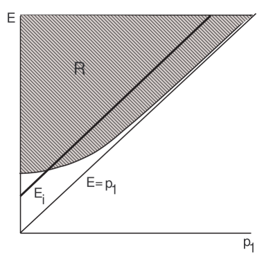
Figure 1: $\cal R$ is the region covered by all final energy curves $E_{f}^{\alpha,\beta,p_{3}}(p_{1})$ for some fixed $p_{2}$, with $p_{4}$ determined by momentum conservation. The curve $E_{i}(p_{1})$ is the initial energy for the same fixed $p_{2}$. Where the latter curve lies inside $\cal R$ there is a solution to the energy and momentum conservation equations.

This graphical representation demonstrates that in any threshold configuration (lower or upper) occuring at some $p_{1}$, the parameters $(\alpha,\beta,p_{3})$ are such that the final energy function $E_{f}^{\alpha,\beta,p_{3}}(p_{1})$ is minimized. That is, the configuration always yields the minimum final particle energy configuration conserving momentum at fixed $p_{1}$ and $p_{2}$. From this fact, it is easy to deduce two general properties of these configurations:

1. All thresholds for processes with two outgoing particles occur at parallel final momenta ($\beta=0$).

2. For a two-particle initial state the momenta are antiparallel at threshold ($\alpha=\pi$).

These properties are in agreement with the well known case of Lorentz invariant kinematics. Nevertheless, LV thresholds can exhibit new features not present in the Lorentz invariant theory, in particular upper thresholds and asymmetric pair creation.

Figure 1 clearly shows that LV allows for a reaction to not only to start at some lower threshold but also to end at some upper threshold where the curve $E_{i}$ exits the region $\cal R$. It can even happen that $E_{i}$ enters and exits $\cal R$ more than once, in which case there are what one might call “local” lower and and upper thresholds.

Another interesting novelty is the possibility to have a (lower or upper) threshold for pair creation with an unequal partition of the initial momentum $p_{in}$ into the two outgoing particles (i.e. $p_{3}\neq p_{4}\neq p_{in}/2$). Equal partition of momentum is a familiar result of Lorentz invariant physics, which follows from the fact that the final particles are all at rest in the zero-momentum frame at threshold. This has often been (erroneously) presumed to hold as well in the presence of LV dispersion relations.

A reason for the occurrence of asymmetric LV thresholds can be seen graphically, as shown in Figure 2. Suppose the dispersion relation for a massive outgoing particle $E_{out}({\bf p})$ has negative curvature at $p=p_{in}/2$, as might be the case for negative LV coefficients. Then a small momentum-conserving displacement from a symmetric configuration can lead to a net decrease in the final state energy. According to the result established above, the symmetric configuration cannot be the threshold one in such a case. A lower $p_{1}$ could satisfy both energy and momentum conservation with an asymmetric final configuration.

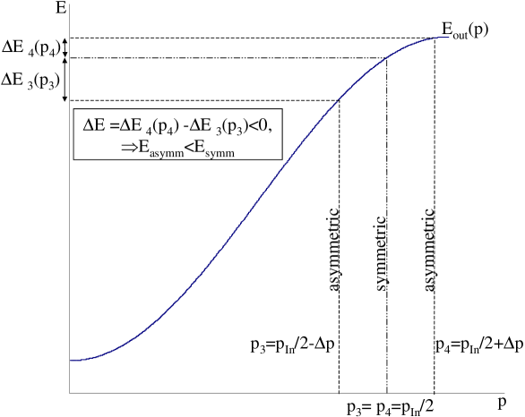
Figure 2: Asymmetric pair production. The negative curvature of the outgoing particle dispersion relation allows the energy of the outgoing pair to be reduced by distributing the initial momentum $p_{in}$ un-equally between the two particles.

A sufficient condition for the pair-creation threshold configuration to be asymmetric is that the final particle dispersion relation has negative curvature at $p=p_{in}/2$. This condition is not necessary however, since it could happen that the energy is locally but not globally minimized by the symmetric configuration.

5 Constraints

Observable effects of LV arise, among other things, from 1) sidereal variation of LV couplings due to motion of the laboratory relative to the preferred frame, 2) dispersion and birefringence of signals over long travel times, 3) anomalous reaction thresholds. We will often express the constraints in terms of the dimensionless parameters $\eta_{n}$ introduced in (5). An order unity value might be considered to be expected in Planck suppressed LV.

The possibility of interesting constraints in spite of Planck suppression arises in different ways for the different types of observations. In the laboratory experiments looking for sidereal variations, the enormous number of atoms allow variations of a resonance frequency to be measured extremely accurately. In the case of dispersion or birefringence, the enormous propagation distances would allow a tiny effect to accumulate. In the anomalous threshold case, the creation of a particle with mass $m$ would be strongly affected by a LV term when the momentum becomes large enough for this term to be comparable to the mass term in the dispersion relation.

We briefly mention first constraints on the renormalizable Standard Model Extension, then focus on LV suppressed by one or two powers of the ratio $E/M$.

5.1 Constraints on renormalizable terms

For the $n=2$ term in (4,5), the absence of a strong threshold effect yields a constraint $\eta_{2}\lesssim(m/p)^{2}(M/\mu)$. If we consider protons and put $\mu=m=m_{p}\sim 1$ GeV, this gives an order unity constraint when $p\sim\sqrt{mM}\sim 10^{19}$ eV. Thus the GZK threshold, if confirmed, can give an order unity constraint, but multi-TeV astrophysics yields much weaker constraints. The strongest laboratory constraints on dimension three and four operators come from clock comparison experiments using noble gas masers Bear:2000cd . The constraints limit a combination of the coefficients for dimension three and four operators for the neutron to be below $10^{-31}$ GeV (the dimension four coefficients are weighted by the neutron mass, yielding a constraint in units of energy). For more on such constraints see e.g. AKbook ; Bluhm:2003ne . Astrophysical limits on photon vacuum birefringence give a bound on the coefficients of dimension four operators of $10^{-32}$ KM .

5.2 Summary of constraints on LV in QED at $O(E/M)$

Since we do not assume universal LV coefficients, different constraints cannot be combined unless they involve just the same particle types. To achieve the strongest combined constraints it is thus preferable to focus on processes involving a small number of particle types. It also helps if the particles are very common and easy to observe. This selects electron-photon physics, i.e. QED, as a useful arena.

The current constraints on the three LV parameters at order $E/M$—one in the photon dispersion relation and two in the electron dispersion relation—will now be summarized. These are equivalent to the parameters in the dimension five operators (8) written down by Myers and Pospelov.

For $n=3$, a strong effect on energy thresholds involving only electrons and photons can occur when the LV term $\eta p^{3}/M$ in the electron or photon dispersion relation is comparable to or greater than the electron mass term $m^{2}$. This happens when

$$p\simeq 14\,{\rm TeV}\,\eta_{3}^{-1/3}.$$ (12)

We can thus obtain order unity and even much stronger constraints from high energy astrophysics, where such energies are reached and exceeded.

In Fig. 3 (from Ref. JLMS ) constraints on the photon ($\xi$) and electron ($\eta$) LV parameters are plotted on a logarithmic scale to allow the vastly differing strengths to be simultaneously displayed. For negative parameters, the negative of the logarithm of the absolute value is plotted, and a region of width $10^{-18}$ is excised around each axis. The synchrotron and Čerenkov constraints must both be satisfied by at least one of the four quantities $\pm\eta_{\pm}$. The IC and synchrotron Čerenkov lines are truncated where they cross. Prior photon decay and absorption constraints are shown in dashed lines since they do not account for the EFT relations between the LV parameters.

We now briefly review the physics and observations behind these and other constraints.

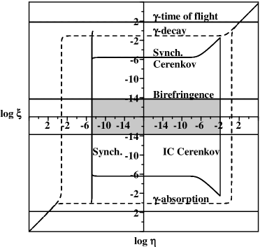
Figure 3: Constraints on LV in QED at $O(E/M)$ (figure from Ref. JLMS ).

Electron helicity dependence and “helicity decay”

The constraint $|\eta_{+}-\eta_{-}|<4$ on the difference between the positive and negative electron helicity parameters was deduced by Myers and Pospelov MP using a previous spin-polarized torsion pendulum experiment Heckel that looked for diurnal changes in resonance frequency. They also determined a numerically stronger constraint using nuclear spins, however this involves four different LV parameters, one for the photon, one for the up-down quark doublet, and one each for the right handed up and down quark singlets. It also requires a model of nuclear structure.

It is possible that an interesting constraint could be obtained from the process of “helicity decay”JLMS . If $\eta_{+}$ and $\eta_{-}$ are unequal, say $\eta_{+}>\eta_{-}$, then a positive helicity electron can decay into a negative helicity electron and a photon, even when the LV parameters do not permit the vacuum Čerenkov effect. In this process, the large $R$ or small ($O(m/E)$) $L$ component of a positive helicity electron is coupled to the small $R$ or large $L$ component of a negative helicity electron respectively. Such “helicity decay” has no threshold energy, so whether this process can be used to set a constraint is solely a matter of the decay rate. It can be shown (assuming $|\xi|\lesssim 10^{-3}$) that for electrons of energy less than the transition energy $(m^{2}M/(\eta_{+}-\eta_{-}))^{1/3}$, the lifetime of an electron susceptible to helicity decay is greater than $4\pi M/(\eta_{+}-\eta_{-})e^{2}m^{2}$. At the limit of the best current bound $|\eta_{+}-\eta_{-}|<4$, the transition energy is approximately 10 TeV and the lifetime for electrons below this energy is greater than $10^{4}$ seconds. This is long enough to preclude any terrestrial experiments from seeing the effect. The lifetime above the transition energy is instead bounded below by $E/e^{2}m^{2}$, which is $10^{-11}$ seconds for energies just above 10 TeV. The lifetime might therefore be short enough to provide new constraints. Such a constraint might come from the Crab Nebula, as explained below.

Vacuum bifrefringence

The birefringence constraint arises from the fact that the LV parameters for left and right circular polarized photons are opposite (10). The phase velocity thus depends on both the wavevector and the helicity. Linear polarization is therefore rotated through an energy dependent angle as a signal propagates, which depolarizes any initially linearly polarized signal. Hence the observation of linearly polarized radiation coming from far away can constrain the magnitude of the LV parameter.

In more detail, with the dispersion relation (10) the direction of linear polarization is rotated through the angle

$$\theta(t)=\left[\omega_{+}(k)-\omega_{-}(k)\right]t/2=\xi k^{2}t/2M$$ (13)

for a plane wave with wave-vector $k$ over a propagation time $t$. The difference in rotation angles for wave-vectors $k_{1}$ and $k_{2}$ is thus

$$\Delta\theta=\xi(k_{2}^{2}-k_{1}^{2})d/2M,$$ (14)

where we have replaced the time $t$ by the distance $d$ from the source to the detector (divided by the speed of light). Note that the effect is quadratic in the photon energy, and proportional to the distance traveled.

This effect has been used to constrain LV in the dimension three (Chern-Simons) CFJ , four KM and five GK ; JLMS ; Mitro terms. The constraint shown in the figure derives from the recent report CB03 of a high degree of polarization of MeV photons from GRB021206. The data analysis has been questioned RF03 , so we shall have to wait and see if it is confirmed. The next best constraint on the dimension five term was deduced by Gleiser and Kozameh GK using UV light from distant galaxies. While ten orders of magnitude weaker, it is still very strong, $|\xi|\lesssim 2\times 10^{-4}$.

Photon time of flight

Photon time of flight constraints Schaefer limit differences in the arrival time at Earth for photons originating in a distant event Pavlopoulos ; GAC-Nat . Time of flight can vary with energy since the LV term in the group velocity is $\xi k/M$. The arrival time difference for wave-vectors $k_{1}$ and $k_{2}$ is thus

$$\Delta t=\xi(k_{2}-k_{1})d/M,$$ (15)

which is proportional to the energy difference and the distance travelled. Using the EFT result (10), the velocity difference of the two polarizations at a given energy is $2|\xi|k/M$, at least twice as large as the one arising from energy differences. However, the time of flight constraint remains many orders of magnitude weaker than the birefringence one from polarization rotation. In Fig. 3 we use the EFT improvement of the constraint of Biller et al. Schaefer (this is the best constraint to date for which a reliable distance is known), which yields $|\xi|<63$.

Vacuum Čerenkov effect, inverse Compton electrons

In the presence of LV the process of vacuum Čerenkov radiation $e\rightarrow e\gamma$ can occur. For example, if the photon dispersion is unmodified and the electron parameter $\eta$ (for one helicity) is positive, then the electron group velocity $v_{g}=1-(m^{2}/2p^{2})+(\eta p/M)+\cdots$ exceeds the speed of light when

$$p_{\rm th}=(m^{2}M/2\eta)^{1/3}\simeq 11\,{\rm TeV}\,\eta^{-1/3}.$$ (16)

This turns out to be the threshold energy for the vacuum Čerenkov process with emission of a zero energy photon, which we call the soft Čerenkov threshold. There is also the possibility of a hard Čerenkov thresholdJacobson:2002hd ; KonMaj . For example, if the electron dispersion is unmodified and the photon parameter $\xi$ is negative then at sufficiently high electron energy the emission of an energetic positive helicity photon is possible. This hard Čerenkov threshold occurs at $p_{\rm th}=(-4m^{2}M/\xi)^{1/3}$, and the emitted photon carries away half the incoming electron momentum. It turns out that the threshold is soft when both $\eta>0$ and $\xi\geq-3\eta$, while it is hard when both $\xi<-3\eta$ and $\xi<\eta$. The hard threshold in the general case is given by $p_{\rm th}=(-4m^{2}M(\xi+\eta)/(\xi-\eta)^{2})^{1/3}$, and the photon carries away a fraction $(\xi-\eta)/2(\xi+\eta)$ of the incoming momentum. In the general case at threshold, neither the incoming nor outgoing electron group velocity is equal to the photon group velocity, so the hard Čerenkov effect cannot simply be interpreted as being due to faster than light motion of a charged particle.

The inverse Compton (IC) Čerenkov constraint uses the electrons of energy up to 50 TeV inferred via the observation of 50 TeV gamma rays from the Crab nebula which are explained by IC scattering. (The implications of a possible high energy population of positrons is discussed below.) Since the vacuum Čerenkov rate is orders of magnitude higher than the IC scattering rate, that process must not occur for these electrons CGlong ; Jacobson:2002hd . The absence of the soft Čerenkov threshold up to 50 TeV produces the vertical IC Čerenkov line in Fig. 3. One can see from (16) that this yields a constraint on $\eta$ of order $(11~{}{\rm TeV}/50~{}{\rm TeV})^{3}\sim 10^{-2}$. It could be that only one electron helicity produces the IC photons and the other loses energy by vacuum Čerenkov radiation. Hence we can infer only that at least one of $\eta_{+}$ and $\eta_{-}$ satisfies the bound.

We do not indicate the hard IC Čerenkov threshold constraint in Fig. 3 since it is superceded by the hard synchrotron Čerenkov constraint discussed below.

Crab synchrotron emission

A constraint complementary to the Čerenkov one was derived in Crab by making use of the very high energy electrons that produce the highest frequency synchrotron radiation in the Crab nebula. For negative values of $\eta$ the electron has a maximal group velocity less than the speed of light, hence there is a maximal synchrotron frequency that can be produced regardless of the electron energy Crab . In the Lorentz invariant case these electrons must have an energy of at least 1500 TeV, which suggests that we should be able to obtain a constraint many orders of magnitude stronger than the IC Čerenkov one. We now explain how this indeed comes about.

Cycling electrons in a magnetic field $B$ emit synchrotron radiation with a spectrum that sharply cuts off at a frequency $\omega_{c}$ given by the formula

$$\omega_{c}=\frac{3}{2}eB\frac{\gamma^{3}(E)}{E}\,,$$ (17)

where $\gamma(E)=(1-v^{2}(E)/c^{2})^{-1/2}$. Here $v(E)$ is the electron group velocity, and $c$ is the usual low energy speed of light. (As shown in Crab the photon energy is low enough to neglect any possible LV correction as long as $|\xi|\lesssim 10^{11}(-\eta)^{4/3}$.) The formula (17) is based on the electron trajectory for a given energy in a given magnetic field, the radiation produced by a given current, and the relativistic relation between energy and velocity. As explained in Crab , and also in some more detail in Jacobson:2003ty (which was written in response to the criticism of GAC-crit ), only the last of these ingredients is significantly affected by LV in the EFT framework we are considering. Hence (17) holds in that framework.

In standard relativistic physics, $E=\gamma m$, so the energy dependence in (17) is entirely through the factor $\gamma^{2}$, which grows without bound as the energy grows. In the LV case, the maximum synchrotron frequency $\omega_{c}^{\rm max}$ is obtained by maximizing $\omega_{c}$ (17) with respect to the electron energy, which amounts to maximizing $\gamma^{3}(E)/E$. Using the difference of group velocities

$$c-v(E)\simeq\frac{m^{2}}{2E^{2}}-\eta\,\frac{E}{M},$$ (18)

we find that this maximization yields

$$\omega_{c}^{\rm max}=0.34\,\frac{eB}{m}(-\eta m/M)^{-2/3}.$$ (19)

This maximum frequency is attained at the energy $E_{\rm max}=(-2m^{2}M/5\eta)^{1/3}=10\,(-\eta)^{-1/3}$ TeV. This is higher than the energy that produces the same cutoff frequency in the Lorentz invariant case, but only by a factor of order unity.

The rapid decay of synchrotron emission at frequencies larger than $\omega_{c}$ implies that most of the flux at a given frequency in a synchrotron spectrum is due to electrons for which $\omega_{c}$ is above that frequency. Thus $\omega_{c}^{\rm max}$ must be greater than the maximum observed synchrotron emission frequency $\omega_{\rm obs}$. This yields the constraint

$$\eta>-\frac{M}{m}\left(\frac{0.34\,eB}{m\omega_{\rm obs}}\right)^{3/2}.$$ (20)

The Crab synchrotron emission has been observed to extend at least up to energies of about 100 MeV AA96 , just before the inverse Compton hump begins to contribute to the spectrum. The magnetic field in the emission region has been estimated by several methods which agree on a value between 0.15–0.6 mG (see e.g. Hillas and references therein.) Two of these methods, radio synchrotron emission and equipartition of energy, are insensitive to Planck suppressed Lorentz violation, hence we are justified in adopting a value of this order for the purpose of constraining Lorentz violation. We use the largest value 0.6 mG for $B$, since it yields the weakest constraint.

Our prior work assumed the high energy Crab radiation was produced purely by electrons, not positrons. We consider here first this case. Then we infer that at least one of the two parameters $\eta_{\pm}$ must be greater than $-7\times 10^{-8}$. We cannot constrain both $\eta$ parameters in this way since it could be that all the Crab synchrotron radiation is produced by electrons of one helicity.

Combined synchrotron & IC Čerenkov constraint

The $\eta$ satisfying the synchrotron constraint must be the same $\eta$ as satisfies the IC Čerenkov constraint discussed above. If the synchrotron $\eta$ did not satisfy the IC Čerenkov constraint, the energy of these synchrotron electrons would necessarily be under 50 TeV, rather than over the Lorentz invariant value of 1500 TeV. The Crab spectrum is well accounted for with a single population of electrons responsible for both the synchrotron radiation and the IC $\gamma$-rays. If there were enough extra electrons to produce the observed synchrotron flux with thirty times less energy per electron, then the electrons of the other helicity, would be equally numerous and would therefore produce too many IC $\gamma$-rays JLMS . It is important that the same $\eta$, i.e.  either $\eta_{+}$ or $\eta_{-}$, satisfies both the synchrotron and the IC Čerenkov constraints. Otherwise, both constraints could have been satisfied by having one of these two parameters arbitrarily large and negative, and the other arbitrarily large and positive.

Possible helicity dependence constraint

As alluded to above, a constraint on helicity dependence of the electron parameter $\eta$ might be possible using the Crab Nebula. Suppose that $\eta_{-}$ is below the synchrotron constraint (i.e. $\eta_{-}<-7\times 10^{-8}$), so that $\eta_{+}$ must satisfy both the synchrotron and Čerenkov constraints as explained above. Then positive helicity electrons must have an energy of at least 50 TeV to produce the observed synchrotron radiation. These must not decay to negative helicity electrons (since those would be unable to produce the synchrotron emission). This would require that the transition energy (discussed inthe helicity dependence section above) be greater than 50 TeV if the decay rate is fast enough. This would yield the constraint $\eta_{+}-\eta_{-}<10^{-2}$.

Possible role of positrons

If the population of high energy charges includes positrons as well as electrons, as in some modelsalice , then the above constraint analysis must be modified. The reasoning discussed so far implies only that at least one of the four parameters $\pm\eta_{\pm}$ satisfies both the synchrotron and IC Čerenkov constraints, since the emitting charge could be either an electron or a positron. In effect, this reduces to the statement that one of $|\eta_{\pm}|$ satisfies the IC Cerenkov constraint. We are currently investigating what constraints can be inferred if the amount of radiation produced by each of the four populations of charges is accounted for more quantitatively.

Vacuum Čerenkov effect, synchrotron electrons

The existence of the synchrotron producing electrons can be exploited to extend the vacuum Čerenkov constraint. For a given $\eta$ satisfying the synchrotron bound, some definite electron energy $E_{\rm synch}(\eta)$ must be present to produce the observed synchrotron radiation. (This is higher for negative $\eta$ and lower for positive $\eta$ than the Lorentz invariant value Crab .) Values of $|\xi|$ for which the vacuum Čerenkov threshold is lower than $E_{\rm synch}(\eta)$ for either photon helicity can therefore be excluded JLMS . This is always a hard photon threshold, since the soft photon threshold occurs when the electron group velocity reaches the low energy speed of light, whereas the velocity required to produce any finite synchrotron frequency is smaller than this.

Photon decay

In the presence of LV the process of photon decay $\gamma\rightarrow e^{+}e^{-}$ can occur. For example, if the electron dispersion is unmodified and the photon parameter $\xi$ is positive, the positive helicity photon decays above the threshold energy $k_{\rm th}=(4m^{2}M/\xi)^{1/3}$. If instead the photon dispersion is unmodified and if electron and positron have the same dispersion with $\eta<0$, then the threshold occurs at $k_{\rm th}=(-8m^{2}M/\eta)^{1/3}$. The threshold for general $\xi$ and $\eta$ is found in Refs. Jacobson:2002hd ; KonMaj .

Contrary to relativistic intuition, it turns out that when $\eta<\xi<0$ the electron and positron are not created with the same momentum. The reason (cf. section 4) is the electron and positron energy functions $E(p)$ have negative curvature at the threshold value of $p$. If the two momenta were equal, the energy of the final state at fixed momentum could be lowered by making the momentum of one particle smaller and one larger by an equal amount.

Previous work on observational constraints using photon decay and photon absorption (to be discussed below) were carried out before it was known how the dispersion depends on helicity and particle vs. anti-particle. Since these constraints are in any case not competitive now with others, we have not attempted to fully account for these relations. Here we just make a few remarks.

The strongest limit on photon decay came from the highest energy photons known to propagate, which at the moment are the 50 TeV photons observed from the Crab nebula Jacobson:2002hd ; KonMaj . These photons must not decay before reaching the earth, so we can rule out those LV parameters that lead to a threshold below 50 TeV, provided the decay rate is fast enough.

Since we do not know the polarization of the observed photons however, we can only exclude regions where both photon polarizations decay. Recall that according to (10) positive and negative helicity photons have opposite parameters $\pm\xi$. A positive helicity photon carries a spin angular momentum of one along the direction of motion. At threshold, where all momenta are aligned, the electron and positron must therefore both have positive helicity. Likewise a left-handed photon decays at threshold into a negative helicity pair. Consider first the case $\eta_{-}=-\eta_{+}$ so that, according to (11), the electron and positron have the same dispersion parameter. Then the outgoing pair both have parameter $\eta_{+}$ for a positive helicity incoming photon and $-\eta_{+}$ for a negative helicity one. We can then exclude those parameters for which both $(\xi,\eta_{+})$ and $(-\xi,-\eta_{+})$ lead to photon decay thresholds below 50 TeV. The allowed region is the intersection of that from the old photon decay constraint Jacobson:2002hd ; KonMaj with its reflection about the $\xi$ and $\eta$ axes. It is a pair of wedges in the upper-right and bottom left quadrants. Numerical work shows that this wedge pattern is maintained for different choices of $\eta_{-}$ relative to $\eta_{+}$, however the exact orientation and shape of the wedges varies. A complete analysis of constraints would also require examination of above threshold processes when the outgoing particles have orbital angular momentum and hence helicities that are not determined solely by the incoming photon.

Photon absorption

A process related to photon decay is photon absorption, $\gamma\gamma\rightarrow e^{+}e^{-}$. Unlike photon decay, this is allowed in Lorentz invariant QED. If one of the photons has energy $\omega_{0}$, the threshold for the reaction occurs in a head-on collision with the second photon having the momentum (equivalently energy) $k_{\rm LI}=m^{2}/\omega_{0}$. For $k_{\rm LI}=10$ TeV (which will be relevant for the observational constraints) the soft photon threshold $\omega_{0}$ is approximately 25 meV, corresponding to a wavelength of 50 microns.

In the presence of Lorentz violating dispersion relations the threshold for this process is in general altered, and the process can even be forbidden. Moreover, as noticed by Kluźniak Kluzniak , in some cases there is an upper threshold beyond which the process does not occur. The lower and upper thresholds for photon annihilation as a function of the two parameters $\xi$ and $\eta$ were obtained in Jacobson:2002hd , before the helicity dependence required by EFT was appreciated. As the soft photon energy is low enough that its LV can be ignored, this corresponds to the case where electrons and positrons have the same LV terms. The analysis is rather complicated. In particular it is necessary to sort out whether the thresholds are lower or upper ones, and whether they occur with the same or different pair momenta.

The photon absorption constraint, neglecting helicity dependent effects, came from the fact that LV can shift the standard QED threshold for annihilation of multi-TeV $\gamma$-rays from nearby blazars, such as Mkn 501, with the ambient infrared extragalactic photons Kluzniak ; GAC-Pir ; SG ; Jacobson:2002hd ; KonMaj ; Jacobson:2003ty ; S03 . LV depresses the rate of absorption of one photon helicity, and increases it for the other. Although the polarization of the $\gamma$-rays is not measured, the possibility that one of the polarizations is essentially unabsorbed appears to be ruled out by the observations which show the predicted attenuation S03 . The electron and positron spin angular momenta add to at most one. At threshold, where the collision is head-on, the photons must therefore have opposite helicity, and hence the electron and positron have opposite helicity. According to (11), they therefore have opposite LV parameters. The threshold analysis has not been redone to account for this.

Vacuum photon splitting

Another forbidden QED process that is allowed in the presence of LV is vacuum photon splitting into $N$ photons, $\gamma\rightarrow N\gamma$. Unlike the other processes considered here, this would be a loop effect. The lowest order Feynman diagram contributing would be a fermion loop with various photon lines attached. The process has no threshold, so whether or not it can be used to set constraints depends on the rate.

Aspects of vacuum photon splitting have been examined in Jacobson:2002hd ; othersplitting . An estimate of the rate, independent of the particular form of the Lorentz violating theory, was given in Ref. Jacobson:2002hd . It was argued that a lower bound on the lifetime is $\delta^{-4}E^{-1}$, where $\delta$ is a Lorentz violating factor. For a photon of energy 50 TeV, this is $10^{-29}\delta^{-4}$ seconds. Such 50 TeV photons arrive from the Crab nebula, about $10^{13}$ seconds away, so the best constraint (i.e. if there is is no further small parameter such as $\alpha^{N}$ or $1/16\pi^{2}$ in the decay rate) we could possibly get on $\delta$ from photon splitting is $\delta\lesssim 10^{-10}$.

For a $p^{n}$ LV term with $n=2$ in the dispersion relation, this is not competitive with the other constraints already obtained. For higher $n$, each contribution arising from an operator of dimension greater than four will be suppressed by at least one inverse power of the scale $M$. For example, contributions from $n=3$ would yield $\delta\sim\xi E/M$. In this case the strongest conceivable constraint on $\xi$ would be of order $\xi\lesssim 10^{4}$, and even this is not competitive with the other constraints.

5.3 Constraints at $O(E/M)$ from UHE cosmic rays

If ultra-high energy cosmic rays (UHECR) are (as commonly assumed) protons, then we can derive strong constraints on $n=3$ type dispersion by a) the absence of a vacuum Čerenkov effect at GZK energies and b) the position of the GZK cutoff. For a soft emitted photon with a long wavelength, the partonic structure of a UHECR proton is presumably irrelevant. In this case we can treat the proton as a point particle as in the QED analysis. With a GZK proton of energy $5\times 10^{19}$ GeV the constraint from the absence of a vacuum Čerenkov effect is $\eta<O(10^{-14})$. For a hard emitted photon, the partonic nature of the proton is important and the relevant mass scale will involve the quark mass. The exact calculation considering the partonic structure for $n=3$ has not been performed, however the threshold region will be similar to that in Jacobson:2002hd . The allowed region in the $\eta-\xi$ plane will be bounded on the right by the $\xi$ axis (within a few orders of magnitude of $10^{-14}$) and below by the line $\xi=\eta$ Jacobson:2002hd . These constraints apply to only one helicity of proton and photon, since the UHECR could consist all of a single helicity. Also the different quarks could have different dispersion parameters. See however section 5.4 for remarks on the approach of Gagnon:2004xh which can be applied to deduce combined constraints in this case.

If the GZK cutoff is observed in its predicted place, this will place limits on the parameters $\eta_{p}$ and $\eta_{\pi}$. For example, if the GZK cutoff is eventually observed to be somewhere between 2 and 7 times $10^{19}$ GeV then there are strong constraints of $O(10^{-11})$ on $\eta_{p}$ and $\eta_{\pi}$ Jacobson:2002hd . As a final comment, an interesting possible consequence of LV is that with upper thresholds, one could possibly reconcile the AGASA and Hi-Res/Fly’s Eye experiments. Namely, one can place an upper threshold below $10^{21}$ GeV while keeping the GZK threshold near $5\times 10^{19}$ GeV. Then the cutoff would be “seen” at lower energies but extra flux would still be present at energies above $10^{20}$ GeV, potentially explaining the AGASA results Jacobson:2002hd . The region of parameter space for this scenario is terribly small, however, again of $O(10^{-11})$.

5.4 Constraints at $O(E^{2}/M^{2})$?

As previously mentioned, CPT symmetry alone could exclude the dimension five LV operators that give $O(E/M)$ modifications to particle dispersion relation, and in any case the constraints on those have become nearly definitive. Hence it is of interest to ask about the $O(E^{2}/M^{2})$ modifications. We close with a brief discussion of the constraints that might be possible on those, i.e. constraints at $O(E^{2}/M^{2})$.

As discussed above, the strength of constraints can be estimated by the requirement $\eta_{4}p^{4}/M^{2}\lesssim m^{2}$, which yields

$$\eta_{4}\lesssim\left(\sqrt{\frac{m}{1\,{\rm eV}}}\frac{100\,{\rm TeV}}{p}\right)^{4}.$$ (21)

Thus, for electrons, an energy around $10^{17}$ eV is needed for an order unity constraint on $\eta_{4}$, and we are probably not going to see any effects directly from such electrons.

For protons an energy $\sim 10^{18}$ eV is needed. This is well below the UHE cosmic ray energy cutoff, hence if and when Auger Auger confirms the identity of UHE cosmic rays as protons at the GZK cutoff, we will obtain an impressive constraint of order $\eta_{4}\lesssim 10^{-5}$ from the absence of vacuum Čerenkov radiation for $10^{20}$ eV protons. From the fact that the GZK threshold is not shifted, we will obtain a constraint of order $\eta_{4}\gtrsim-10^{-2}$, assuming equal $\eta_{4}$ values for proton and pion.

In fact, if one assumes the cosmic rays near but below the GZK cutoff are hadrons, one already obtains a strong bound Gagnon:2004xh . Depending on the species dependence of the LV coefficients, bounds of order $10^{-2}$ or better can be placed on $\eta_{4}$. The bounds claimed in  Gagnon:2004xh are actually two sided, and it is worthwhile to explain how such bounds come about for a single source particle. Up to this point it has been necessary to use at least two reactions with different source particles to derive a two sided bounds. For example, the Crab constraints rely on the existence of both 50 TeV electrons and photons, treating each as a fundamental particle with its own LV coefficient. In contrast, the two sided bounds in Gagnon:2004xh are derived by using a parton model for particles where the LV coefficients apply to the constituent partons. By considering many different outgoing particle spectra from an incoming hadron in combination with the parton approach the authors of Gagnon:2004xh are able to find sets of reactions that yield two sided bounds. Hence, the parton approach is extremely useful as it dramatically increases the number of constraints that can be derived from a single incoming particle. However, it also requires more assumptions about the behavior of the parton distributions at cosmic ray energies.

Impressive constraints might also be obtained from the absence of neutrino vacuum Čerenkov radiation: putting in 1 eV for the mass in (21) yields an order unity constraint from 100 TeV neutrinos, but only if the Čerenkov rate is high enough. The rate will be low, since it proceeds only via the non-local charge structure of the neutrino. Recent calculations Dave? have shown that the rate is not high enough at that energy. However, for $10^{20}$ eV UHE neutrinos, which may be observed by the proposed EUSO and/or OWL satellite observatories, the rate will be high enough to derive a strong constraint. The value of the constraint would depend on the emission rate, which has not yet been computed. For a gravitational Čerenkov reaction, the rate (which is lower but easier to compute than the electromagnetic rate) would be high enough for a neutrino from a distant source to radiate provided $\eta_{4}\gtrsim 10^{-2}$. Hence in this case one might obtain a constraint of order $\eta_{4}\lesssim 10^{-2}$, or stronger in the electromagnetic case.

A time of flight constraint at order $(E/M)^{2}$ might be possible GACsecgen if gamma ray bursts produce UHE ($\sim 10^{19}$ eV) neutrinos, as some models predict, via limits on time of arrival differences of such UHE neutrinos vs. soft photons (or gravitational waves). Another possibility is to obtain a vacuum birefringence constraint with higher energy photons Mitro , although such a constraint would be less powerful since EFT does not imply that the parameters for opposite polarizations are opposite at order $(E/M)^{2}$. If future GRB’s are found to be polarized at $\sim 100$ MeV, that could provide a birefringence constraint $|\xi_{4+}-\xi_{4-}|\lesssim 1$.

6 Conclusion

At present there are only hints, but no compelling evidence for Lorentz violation from quantum gravity. Moreover, even if LV is present, the use of EFT for its low energy parametrization is not necessarily valid. Nevertheless, we believe that the constraints derived from the simple ideas discussed here are still important. They allow tremendous advances in observational reach to be applied in a straightforward manner to limit reasonable possibilities that might arise from fundamental Planck scale physics. Such guidance is especially welcome for the field of quantum gravity, which until the past few years has had little connection with observed phenomena.

References

- (1) V. F. Mukhanov, H. A. Feldman and R. H. Brandenberger, “Theory Of Cosmological Perturbations. Part 1. Classical Perturbations. Part 2. Quantum Theory Of Perturbations. Part 3. Extensions,” Phys. Rept. 215, 203 (1992).
- (2) G. Amelino-Camelia, “Are we at the dawn of quantum-gravity phenomenology?,” Lect. Notes Phys. 541, 1 (2000) [arXiv:gr-qc/9910089].
- (3) K. Greisen, “End To The Cosmic Ray Spectrum?,” Phys. Rev. Lett. 16, 748 (1966); G. T. Zatsepin and V. A. Kuzmin, “Upper Limit Of The Spectrum Of Cosmic Rays,” JETP Lett. 4, 78 (1966) [Pisma Zh. Eksp. Teor. Fiz. 4, 114 (1966)].
- (4) F. W. Stecker, “Cosmic physics: The high energy frontier,” J. Phys. G 29, R47 (2003) [arXiv:astro-ph/0309027].
- (5) T. Jacobson, S. Liberati and D. Mattingly, “Threshold effects and Planck scale Lorentz violation: Combined constraints from high energy astrophysics,” Phys. Rev. D 67, 124011 (2003) [arXiv:hep-ph/0209264].
- (6) D. De Marco, P. Blasi and A. V. Olinto, “On the statistical significance of the GZK feature in the spectrum of ultra high energy cosmic rays,” Astropart. Phys. 20, 53 (2003) [arXiv:astro-ph/0301497].
- (7) http://www.auger.org/
- (8) S. R. Coleman and S. L. Glashow, “Evading the GZK cosmic-ray cutoff,” [arXiv:hep-ph/9808446]. For previous suggestions relating LV to modification of the GZK cutoff see Kirzhnits and ChechinDirac and Gonzalez-MestresGM .
- (9) O. Gagnon and G. D. Moore, “Limits on Lorentz violation from the highest energy cosmic rays,” arXiv:hep-ph/0404196.
- (10) See, e.g. P. A. M. Dirac, “Is there an aether?,” Nature 168, 906–907 (1951); J. D. Bjorken, “A dynamical origin for the electromagnetic field,” Ann. Phys. 24, 174 (1963); P. Phillips, “Is the graviton a Goldstone boson?,” Physical Review 146, 966 (1966); D.I. Blokhintsev, Usp. Fiz. Nauk. 89, 185 (1966) [Sov. Phys. Usp. 9, 405 (1966)]; L.B. Rédei, “Validity of special relativity at small distances and the velocity dependence of the muon lifetime,” Phys. Rev. 162, 1299-1301 (1967); T. G. Pavlopoulos, “Breakdown Of Lorentz invariance,” Phys. Rev. 159, 1106 (1967); D.A. Kirzhnits and V.A. Chechin, “Ultra-High-Energy Cosmic Rays and a Possible Generaliation of Relativistic Theory,” Yad. Fiz. 15, 1051 (1972) [Sov. J. Nucl. Phys. 15, 585 (1972)].
- (11) G. Amelino-Camelia, “Relativity in space-times with short-distance structure governed by an observer-independent (Planckian) length scale,” Int. J. Mod. Phys. D 11, 1643 (2002) [arXiv:gr-qc/0210063].
- (12) C.M. Will and K. Nordvedt, Jr., “Conservation Laws and Preferred Frames in Relativistic Gravity. I. Preferred-Frame Theories and an Extended PPN Formalism,” Astrophys. J. 177, 757 (1972); K. Nordvedt, Jr. and C.M. Will, “Conservation Laws and Preferred Frames in Relativistic Gravity. II. Experimental Evidence to Rule Out Preferred-Frame Theories of Gravity,” Astrophys. J. 177, 775 (1972); R.W. Hellings and K. Nordvedt, Jr., “Vector-metric theory of gravity,” Phys. Rev. D7, 3593 (1973).
- (13) H. B. Nielsen and M. Ninomiya, “Beta Function In A Noncovariant Yang-Mills Theory,” Nucl. Phys. B 141, 153 (1978); S. Chadha and H. B. Nielsen, “Lorentz Invariance As A Low-Energy Phenomenon,” Nucl. Phys. B 217, 125 (1983); H. B. Nielsen and I. Picek, “Lorentz Noninvariance,” Nucl. Phys. B 211, 269 (1983) [Addendum-ibid. B 242, 542 (1984)]; J. R. Ellis, M. K. Gaillard, D. V. Nanopoulos and S. Rudaz, “Uncertainties In The Proton Lifetime,” Nucl. Phys. B 176, 61 (1980). A. Zee, “Perhaps Proton Decay Violates Lorentz Invariance,” Phys. Rev. D 25, 1864 (1982).
- (14) See, for example, M. Gasperini, “Singularity prevention and broken Lorentz symmetry”, Class. Quantum Grav. 4, 485 (1987); “Repulsive gravity in the very early Universe”, Gen. Rel. Grav. 30, 1703 (1998); and references therein.
-
(15)
T. Jacobson and D. Mattingly, “Generally covariant model of a
scalar field with high frequency dispersion and the cosmological
horizon problem,” Phys. Rev. D 63, 041502 (2001).
[hep-th/0009052];
“Gravity with a dynamical preferred frame,” Phys. Rev. D 64, 024028 (2001). - (16) See M. Haugan and C. Will, Physics Today, May 1987; C.M. Will, Theory and Experiment in Gravitational Physics (Cambridge Univ. Press, 1993), and references therein.
- (17) V. A. Kostelecky and S. Samuel, “Spontaneous Breaking Of Lorentz Symmetry In String Theory,” Phys. Rev. D 39, 683 (1989).
- (18) T. Jacobson, “Black hole evaporation and ultrashort distances,” Phys. Rev. D 44, 1731 (1991).
- (19) W. G. Unruh, “Dumb holes and the effects of high frequencies on black hole evaporation,” Phys. Rev. D 51, 2827-2838 (1995), [arXiv:gr-qc/9409008].
- (20) See J. Martin, this volume; or, e.g., J. Martin and R. Brandenberger, “On the dependence of the spectra of fluctuations in inflationary cosmology on trans-Planckian physics,” Phys. Rev. D 68, 063513 (2003) [arXiv:hep-th/0305161] and references therein.
- (21) L. Gonzalez-Mestres, “Lorentz symmetry violation and high-energy cosmic rays,”, [arXiv:physics/9712005].
- (22) D. Colladay and V. A. Kostelecky, “Lorentz-violating extension of the standard model,” Phys. Rev. D 58, 116002 (1998), [arXiv:hep-ph/9809521].
- (23) V. A. Kostelecky, Proceedings of the Second Meeting on CPT and Lorentz Symmetry, Bloomington, USA, 15-18 August 2001. Singapore, World Scientific (2002).
- (24) M. Takeda et al., “Extension of the cosmic-ray energy spectrum beyond the predicted Greisen-Zatsepin-Kuzmin cutoff,” Phys. Rev. Lett. 81, 1163 (1998) [arXiv:astro-ph/9807193].
- (25) S. R. Coleman and S. L. Glashow, “High-energy tests of Lorentz invariance,” Phys. Rev. D 59, 116008 (1999) [arXiv:hep-ph/9812418].
- (26) G. Amelino-Camelia, J. R. Ellis, N. E. Mavromatos, D. V. Nanopoulos and S. Sarkar, “Potential Sensitivity of Gamma-Ray Burster Observations to Wave Dispersion in Vacuo,” Nature 393, 763 (1998) [arXiv:astro-ph/9712103].
- (27) R. Gambini and J. Pullin, “Nonstandard optics from quantum spacetime,” Phys. Rev. D 59, 124021 (1999) [arXiv:gr-qc/9809038].
- (28) C. N. Kozameh and M. F. Parisi, “Lorentz invariance and the semiclassical approximation of loop quantum gravity,” Class. Quant. Grav. 21, 2617 (2004) [arXiv:gr-qc/0310014].
- (29) J. Alfaro, M. Reyes, H. A. Morales-Tecotl and L. F. Urrutia, “On alternative approaches to Lorentz violation in loop quantum gravity inspired models,” arXiv:gr-qc/0404113.
- (30) R. J. Gleiser and C. N. Kozameh, “Astrophysical limits on quantum gravity motivated birefringence,” Phys. Rev. D 64, 083007 (2001) [arXiv:gr-qc/0102093].
- (31) W. Coburn and S. E. Boggs, “Polarization of the prompt gamma-ray emission from the gamma-ray burst of 6 December 2002,” Nature 423, 415 (2003) [arXiv:astro-ph/0305377].
- (32) R. E. Rutledge and D. B. Fox, “Re-Analysis of Polarization in the Gamma-ray flux of GRB 021206,” [arXiv:astro-ph/0310385]; S. E. Boggs and W. Coburn, “Statistical Uncertainty in the Re-Analysis of Polarization in GRB021206,” [arXiv:astro-ph/0310515]. C. Wigger et al., “Gamma-Ray Burst Polarization: Limits from RHESSI Measurements,” [arXiv:astro-ph/0405525].
- (33) T. A. Jacobson, S. Liberati, D. Mattingly and F. W. Stecker, “New limits on Planck scale Lorentz violation in QED,” Phys. Rev. Lett. 93, 021101 (2004) [arXiv:astro-ph/0309681].
- (34) I. G. Mitrofanov, ”A constraint on canonical quantum gravity”, Nature 426, 139 (2003).
- (35) R. J. Protheroe and H. Meyer, “An infrared background TeV gamma ray crisis?,” Phys. Lett. B 493, 1 (2000) [arXiv:astro-ph/0005349].
- (36) A. K. Konopelko, A. Mastichiadis, J. G. Kirk, O. C. de Jager and F. W. Stecker, “Modelling the TeV gamma-ray spectra of two low redshift AGNs: Mkn 501 and Mkn 421,” Astrophys. J. 597, 851 (2003) [arXiv:astro-ph/0302049].
- (37) R. C. Myers and M. Pospelov, “Experimental challenges for quantum gravity,” Phys. Rev. Lett. 90, 211601 (2003) [arXiv:hep-ph/0301124].
- (38) T. Jacobson, S. Liberati and D. Mattingly, “Lorentz violation and Crab synchrotron emission: A new constraint far beyond the Planck scale,” Nature 424, 1019 (2003) [arXiv:astro-ph/0212190].
- (39) G. Amelino-Camelia, “Improved limit on quantum-spacetime modifications of Lorentz symmetry from observations of gamma-ray blazars,” [arXiv:gr-qc/0212002]; “A perspective on quantum gravity phenomenology,” [arXiv:gr-qc/0402009].
- (40) E. Fischbach, M. P. Haugan, D. Tadic and H. Y. Cheng, “Lorentz Noninvariance And The Eotvos Experiments,” Phys. Rev. D 32, 154 (1985).
- (41) C. P. Burgess, J. Cline, E. Filotas, J. Matias and G. D. Moore, “Loop-generated bounds on changes to the graviton dispersion relation,” JHEP 0203, 043 (2002) [arXiv:hep-ph/0201082].
- (42) J. R. Ellis, N. E. Mavromatos, D. V. Nanopoulos and A. S. Sakharov, “Space-time foam may violate the principle of equivalence,” arXiv:gr-qc/0312044.
- (43) R. Lehnert, “Threshold analyses and Lorentz violation,” Phys. Rev. D 68, 085003 (2003) [arXiv:gr-qc/0304013].
- (44) V. A. Kostelecky and R. Lehnert, “Stability, causality, and Lorentz and CPT violation,” Phys. Rev. D 63, 065008 (2001) [arXiv:hep-th/0012060].
- (45) V. A. Kostelecky and S. Samuel, “Gravitational Phenomenology In Higher Dimensional Theories And Strings,” Phys. Rev. D 40, 1886 (1989).
- (46) A. Perez and D. Sudarsky, “Comments on challenges for quantum gravity,” [arXiv:gr-qc/0306113].
- (47) J. Collins, A. Perez, D. Sudarsky, L. Urrutia and H. Vucetich, “Lorentz invariance: An additional fine-tuning problem,” [arXiv:gr-qc/0403053].
- (48) See e.g. M. Creutz, Quarks, gluons and lattices (Cambridge Univ. Press, 1985); G. Moore, “Informal Lectures on Lattice Gauge Theory,” http://www.physics.mcgill.ca/guymoore/latt_lectures.pdf.
- (49) S. G. Nibbelink and M. Pospelov, “Lorentz violation in supersymmetric field theories,” arXiv:hep-ph/0404271.
- (50) D. Mattingly, T. Jacobson and S. Liberati, “Threshold configurations in the presence of Lorentz violating dispersion relations,” Phys. Rev. D 67, 124012 (2003) [arXiv:hep-ph/0211466].
- (51) D. Bear, R. E. Stoner, R. L. Walsworth, V. A. Kostelecky and C. D. Lane, “Limit on Lorentz and CPT violation of the neutron using a two-species noble-gas maser,” Phys. Rev. Lett. 85, 5038 (2000) [Erratum-ibid. 89, 209902 (2002)] [arXiv:physics/0007049].
- (52) R. Bluhm, “Lorentz and CPT tests in matter and antimatter,” Nucl. Instrum. Meth. B 221, 6 (2004) [arXiv:hep-ph/0308281].
- (53) V. A. Kostelecky and M. Mewes, “Cosmological constraints on Lorentz violation in electrodynamics,” Phys. Rev. Lett. 87, 251304 (2001) [arXiv:hep-ph/0111026]; Phys. Rev. D 66, 056005 (2002) [arXiv:hep-ph/0205211].
- (54) B. R. Heckel et al., “Torsion balance test of spin coupled forces,” Proceedings of the International Conference on Orbis Scientiae, 1999, Coral Gables, (Kluwer, 2000); B. R. Heckel, http://www.npl.washington.edu/eotwash/publications/cpt01.pdf.
- (55) S. M. Carroll, G. B. Field and R. Jackiw, “Limits On A Lorentz And Parity Violating Modification Of Electrodynamics,” Phys. Rev. D 41, 1231 (1990).
- (56) See Pavlopoulos in Dirac .
- (57) B. E. Schaefer, “Severe Limits on Variations of the Speed of Light with Frequency,” Phys. Rev. Lett. 82, 4964 (1999) [astro-ph/9810479]; S. D. Biller et al., “Limits to quantum gravity effects from observations of TeV flares in active galaxies,” Phys. Rev. Lett. 83, 2108 (1999) [arXiv:gr-qc/9810044]; P. Kaaret, “Pulsar radiation and quantum gravity,” Astronomy and Astrophysics, 345, L32-L34 (1999) [arXiv:astro-ph/9903464]; S. E. Boggs, C. B. Wunderer, K. Hurley and W. Coburn, “Testing Lorentz Non-Invariance with GRB021206,” arXiv:astro-ph/0310307, Ap. J. Letters, to appear.
- (58) T. J. Konopka and S. A. Major, “Observational limits on quantum geometry effects,” New J. Phys. 4, 57 (2002) [arXiv:hep-ph/0201184].
- (59) T. Jacobson, S. Liberati and D. Mattingly, “Comments on ‘Improved limit on quantum-spacetime modifications of Lorentz symmetry from observations of gamma-ray blazars’,” [arXiv:gr-qc/0303001].
- (60) F.A. Aharonian, A.M. Atoyan, “On the mechanisms of gamma radiation in the Crab Nebula”, Mon. Not. R. Astron. Soc. 278, 525 (1996).
- (61) A. M. Hillas et al., The Spectrum of TeV gamma rays from the crab nebula, Astrophysical J., 503, 744 (1998).
- (62) A. Harding, “Gamma-ray pulsars: Models and predictions” in High energy gamma-ray astronomy: international symposium Heidelberg, Germany, 26-30 June 2000. Melville, NY, American Institute of Physics (2001) [arXiv:astro-ph/0012268].
- (63) W. Kluzniak, “Transparency Of The Universe To Tev Photons In Some Models Of Quantum Gravity,” Astropart. Phys. 11, 117 (1999).
- (64) G. Amelino-Camelia and T. Piran, “Planck-scale deformation of Lorentz symmetry as a solution to the UHECR and the TeV-gamma paradoxes,” Phys. Rev. D 64, 036005 (2001) [arXiv:astro-ph/0008107].
- (65) F. W. Stecker and S. L. Glashow, “New tests of Lorentz invariance following from observations of the highest energy cosmic gamma rays,” Astropart. Phys. 16, 97 (2001) [arXiv:astro-ph/0102226].
- (66) F. W. Stecker, “Constraints on Lorentz invariance violating quantum gravity and large extra dimensions models using high energy gamma ray observations,” Astropart. Phys. 20, 85 (2003) [arXiv:astro-ph/0308214].
- (67) C. Adam and F. R. Klinkhamer, “Photon decay in a CPT-violating extension of quantum electrodynamics,” Nucl. Phys. B 657, 214 (2003) [arXiv:hep-th/0212028]; V. A. Kostelecky and A. G. M. Pickering, “Vacuum photon splitting in Lorentz-violating quantum electrodynamics,” Phys. Rev. Lett. 91, 031801 (2003) [arXiv:hep-ph/0212382]; C. Adam and F. R. Klinkhamer, “Comment on ‘Vacuum photon splitting in Lorentz-violating quantum electrodynamics’,” arXiv:hep-ph/0312153.
- (68) D. Mattingly and B. McElrath, To be published.
- (69) G. Amelino-Camelia, “Proposal of a second generation of quantum-gravity-motivated Lorentz-symmetry tests: Sensitivity to effects suppressed quadratically by the Planck scale,” Int. J. Mod. Phys. D 12, 1633 (2003) [arXiv:gr-qc/0305057].
- (70) T. Jacobson, S. Liberati and D. Mattingly, “Quantum gravity phenomenology and Lorentz violation,” arXiv:gr-qc/0404067.
Index
- GZK cutoff §2.1
- helicity decay §5.2
- inverse Compton scattering §5.2