Reactor Measurement of $\theta_{12}$;
Principles, Accuracies and Physics Potentials

Abstract

We discuss reactor measurement of $\theta_{12}$ which has a potential of reaching the ultimate sensitivity which surpasses all the methods so far proposed. The key is to place a detector at an appropriate baseline distance from the reactor neutrino source to have an oscillation maximum at around a peak energy of the event spectrum in the absence of oscillation. By a detailed statistical analysis the optimal distance is estimated to be $\simeq(50-70)$ km$\times[8\times 10^{-5}\text{eV}^{2}/\Delta m^{2}_{21}]$, which is determined by maximizing the oscillation effect in the event number distribution and minimizing geo-neutrino background contamination. To estimate possible uncertainty caused by surrounding nuclear reactors in distance of $\sim 100$ km, we examine a concrete example of a detector located at Mt. Komagatake, 54 km away from the Kashiwazaki-Kariwa nuclear power plant in Japan, the most powerful reactor complex in the world. The effect turns out to be small. Under a reasonable assumption of systematic error of 4% in the experiment, we find that $\sin^{2}{\theta_{12}}$ can be determined to the accuracy of $\simeq$ 2% ($\simeq$ 3%), at 68.27% CL for 1 degree of freedom, for 60 GW${}_{\text{th}}\cdot$kton$\cdot$yr (20 GW${}_{\text{th}}\cdot$kton$\cdot$yr) operation. We also discuss implications of such an accurate measurement of $\theta_{12}$.

I Introduction

Reactor neutrino experiments have been the source of rich physics informations review1 . The very existence of (anti-)neutrino was proven by the memorial reactor neutrino experiment by Reines and Cowan reines-cowan . In recent years, reactor neutrino experiments have been playing greater rôle than in any other era of neutrino physics. Following SNO SNO ; sno_salt who has confirmed by the in situ measurement that the solar neutrino deficit is indeed caused by neutrino flavor transformation, KamLAND KamLAND ; KamLAND_new observed clear deficit of reactor neutrinos and pinned down a unique parameter region, the large-mixing-angle (LMA) Mikheyev-Smirnov-Wolfenstein (MSW) solution MSW . Thus, the solar neutrino problem which lasted nearly 40 years has now been solved. At the same time, the basic structure of the (1-2) sector of the lepton flavor mixing matrix, the Maki-Nakagawa-Sakata (MNS) matrix MNS , was determined.

Reactor neutrino experiments also play (and will play) crucial rôle to explore the (1-3) sector of the MNS matrix, the unique sector whose structure is not yet determined. The CHOOZ and the Palo Verde experiments were able to place stringent constraints on $\theta_{13}$ CHOOZ ; PaloVerde . It was recognized that reactor measurement of $\theta_{13}$ has very special characteristics as a pure measurement of $\theta_{13}$, whose property should play an important part in solving the problem of parameter degeneracy MSYIS . It was also stressed that the rôle played by reactor experiments is complementary to those by long-baseline (LBL) accelerator neutrino experiments. The proposal, sometime after an earlier Russian project krasnoyarsk , was followed by a spur of experimental projects over the globe which are now summarized in the White Paper Report reactor_white .

Are those described above all that can be done by reactor neutrino experiments? We answer the question in the negative by proposing dedicated reactor neutrino experiments for precise measurement of $\theta_{12}$ in this paper. We will show that the accuracy attainable by such reactor experiments for $\theta_{12}$ can reach to $\simeq$ 2% for $\sin^{2}\theta_{12}$ for 1 degree of freedom (DOF) under a reasonable assumption of systematic errors. It surpasses those expected by the other methods so far proposed, e.g., by combining KamLAND with accurate ⁷Be and pp solar neutrino measurement bahcall-pena . Throughout this paper, we will demonstrate these statements by careful treatment of the optimization of the baseline distance as well as the effects of geophysical neutrinos (hereafter, geo-neutrinos).

The key idea for such an enormous sensitivity is to place the detector at the appropriate distance to see the effect of oscillation at the place where it is maximal. A zeroth order estimation of the distance BCG03 is given by $L_{\text{OM}}\equiv 2\pi E_{\nu}^{\text{peak}}/\Delta m^{2}_{21}\simeq 63$ km, where $\Delta m^{2}_{21}=7.9\times 10^{-5}\mbox{eV}^{2}$ is the current best fit value KamLAND_new , and $E_{\nu}^{\text{peak}}=4$ MeV is a typical neutrino energy where event rate has a maximum in the absence of oscillation. But, due to the fact that the reactor neutrino energy spectrum is rather broad and the $1/L^{2}$ dependence of the intensity of neutrino flux, the optimal distances turned out to be shorter and spread over a range of 50 to 70 km, adding more variety for the site selection of the detector. We also discuss the geo-neutrino background contamination and its relevance in determining the best position to place the detector.

It seems that now a coherent view of how to determine accurately the “large” mixing angles has emerged. Namely, disappearance measurement at around the oscillation maximum gives the highest sensitivities for both of the large angles, $\theta_{12}$ and $\theta_{23}$. It is well recognized that the most accurate way of determining $\sin^{2}2\theta_{23}$ will be achieved by the next generation LBL accelerator neutrino experiments by using their $\nu_{\mu}$ disappearance mode JPARC ; NuMI ; SPL . In particular, in the JPARC-SK experiment, the accuracy of determination of $\sin^{2}{2\theta_{23}}$ is expected to reach down to $\simeq$ 1% at 90% CL JPARC ; MSS .

What is the scientific merit of such precise measurement of $\theta_{12}$? We will discuss this question in length in Sec. VIII, but here we make only two remarks, one from particle physics and the other from solar physics point of view. Current understanding of nonzero neutrino mass involves, most probably, the existence of a large energy scale where leptons and quarks are unified GUT , whose simplest model realization is the seesaw model seesaw . Various models so far proposed try to relate quark and lepton mass matrix based on the underlying philosophy. For a review see e.g., altarelli . We will probably need detailed informations of lepton mixing matrix which are comparable with that of quarks when we want to test the theory for lepton and quark mixings, which should emerge someday in the future. If the solar angle $\theta_{12}$ is in fact complementary to the Cabibbo angle QLC , there is an immense request for accurate determination of $\theta_{12}$.

What is the solar physics implication of accurate measurement of $\theta_{12}$? The solar neutrino flux measured on the earth inevitably contains the effect of neutrino flavor transformation, and therefore the precision of its determination is affected by the uncertainty of $\theta_{12}$. We thus believe that accurate determination of $\theta_{12}$ has a great merit for precise observational solar astrophysics in which an accurate measurement of the infant flux produced at the solar core is required.

In Sec. II we discuss the basic principle and power of the method of tuning the baseline distance for accurate determination of $\theta_{12}$ by reactor neutrinos. In Sec. III we discuss the requirements and possible obstacle for such reactor $\theta_{12}$ experiments. They include the systematic errors, a possible uncertainty due to geo-neutrino background and the unknown value of $\theta_{13}$. In Sec. IV we describe the analysis procedure and give a quantitative estimate of the optimal baseline distances by fully taking into account the geo-neutrino background. We use a specific setting of the detector to estimate effects of the other surrounding reactors. In Sec. V we carry out the sensitivity analysis. In Sec. VI we examine the stability of our results against changes of our statistical procedure. In Sec. VII we compare the sensitivity of reactor $\theta_{12}$ experiments with the one that will be reached by KamLAND-solar combined method. In Sec. VIII we discuss possible physics implications of a precise measurement of $\theta_{12}$.

II Accurate Measurement of $\theta_{12}$ by Reactors by tuning baseline distance

We discuss in this section the method for accurate determination of $\theta_{12}$ by choosing an appropriate distance to the detector from a principal (nearest) nuclear reactor. We start by giving a pedagogical self-contained description of the basic principle of the measurement. We then contrast the sensitivity achievable by our method with that of KamLAND KamLAND ; KamLAND_new to illuminate the power of the method we propose by explicitly showing improvement over the marvelous experiment using the same neutrino flux from the reactors located all over Japan.

For ease in frequent reference to a dedicated liquid scintillator detector at the distances of 50-70 km, we use in this paper the acronym “SADO” as an abbreviation,

$$\mbox{SADO}\equiv\mbox{Several-tens of km Antineutrino DetectOr}.$$ (1)

II.1 Method for precise measurement of $\theta_{12}$

The secret behind the potentially powerful method is to place a detector to the location where the oscillation effect has its maximum in the observable quantity, i.e., the number of events (not in the probability alone). The optimal distances for a given value of $\Delta m^{2}_{21}$ are

$$L_{\rm optimal}\simeq(50-70)\left[\displaystyle\frac{\Delta m^{2}_{21}}{8\times 10^{-5}\ \text{eV}^{2}}\right]^{-1}\text{km,}$$ (2)

as we will find in Sec. IV after establishing our statistical method (See Fig. 3.) The optimal distance coincides approximately, but not exactly, with the first oscillation maximum (the one encountered first by neutrinos as they travel) for the peak energy of reactor neutrino event distribution. Moreover, such a distance must be established by taking into account background contribution from geo-neutrinos, as we will see in Sec. III.

In Fig.1 we show the range of survival probabilities as a function of neutrino energy in a form of band which is spanned by $P(\bar{\nu}_{e}\rightarrow\bar{\nu}_{e})$ obtained by varying $\sin^{2}\theta_{12}$ between 0.25 (upper end) and 0.35 (lower end). The probabilities are computed using the current best fit value of $\Delta m^{2}_{21}$ and with the two distances $L=50$ (red) and 60 km (blue).

We observe that the oscillation maximum (minimum in the survival probability) occurs at $E_{\nu}\simeq(3.0$-4.0) MeV around the peak energy where the event rate is maximal in the absence of oscillation. The most important feature for us is that the depth of the minimum in the survival probability is the most sensitive place to the variation of $\sin^{2}\theta_{12}$ in the entire figure. Nothing but that property is the key to the enormous accuracy of reactor $\theta_{12}$ measurement to be explored in this paper.

We should note that there were some previous attempts along the similar line of thought. To our knowledge, dedicated reactor experiment for $\theta_{12}$ at the oscillation maximum has first been considered by Takasaki who did a back of the envelope estimation of the sensitivity assuming an appropriate site at $\sim$70 km away from the Fukushima nuclear reactors takasaki . A statistical treatment for estimating the accuracy of $\theta_{12}$ determination was presented by Bandyopadhyay et al. BCG03 which resulted in about 10% error (99% CL, 2 DOF) in $\sin^{2}\theta_{12}$. It is about factor of 2 larger than ours; See Fig. 4. They also did not address the optimization problem of the sensitivity with respect to the baseline distance. A different strategy which utilizes not only the first oscillation maximum but also the subsequent minimum was proposed by Bouchiat bouchiat .

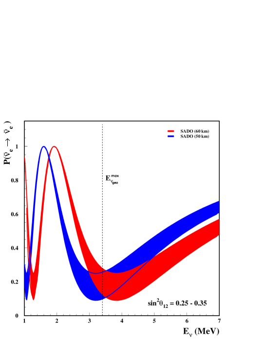
Figure 1: Ranges of the survival probabilities $P(\bar{\nu}_{e}\rightarrow\bar{\nu}_{e})$ of antineutrinos from the nuclear reactor complex as a function of neutrino energy are plotted for two distances to SADO, 50 km (blue) and 60 km (red). The upper and lower boundary of each band corresponds, respectively, to $\sin^{2}\theta_{12}=0.25$ and 0.35. Here $\Delta m^{2}_{21}=7.9\times 10^{-5}$ eV² and $\theta_{13}=0$. The vertical dashed line marks the current KamLAND energy threshold $E_{\nu}=3.4$ MeV for reactor neutrino analysis, which corresponds to the maximum energy for geo-neutrinos.

II.2 Setting

Throughout this paper we analyze simultaneously the two settings:

(A) SADO with single reactor complex, which will be denoted as SADO_single.

(B) SADO with multiple reactor complex, which will be denoted as SADO_multi.

The set up (A) may be an excellent approximation for many reactor sites in the world including Angra reactor in Brazil and Daya Bay in China reactor_white . On the other hand, the set up (B) with multiple reactor complex in addition to the nearest one, which could act as “background”, is inevitable if we think about experiments in Japan, for example, where many nuclear power plants (NPPs) are located within $\sim$ 100 km.

For definiteness, we take a particular site for the set up (B) in this paper; SADO at Mt. Komagatake, Niigata prefecture, Japan, which is about 54 km away from the Kashiwazaki-Kariwa nuclear reactor complex with the maximal thermal power of 24.3 GW_th, the largest NPP in the world. Taking the particular setting is necessary to estimate the “background effects” caused by the other reactors than the nearest one. For the former case (A) one can use any reactor site, but for purpose of comparison, we just switch off contributions from the other 15 reactors except for the Kashiwazaki-Kariwa NPP to use the common normalization factor. In Table 4 in Appendix A, we present the names of the reactor NPPs, their current (near future) thermal power, their distances from KamLAND and from SADO as well as their relative contributions to the neutrino flux at these sites.

To make our analysis useful for experiments at any other reactor sites we present our plots, except for Fig.2, in units of GW${}_{\rm th}\cdot$kt$\cdot$yr where “kt” is an abbreviation of kton. Notice that the number in the unit refers only to the reactor power of the principal reactor, the Kashiwazaki-Kariwa NPP in this paper, and does not include the one from other 15 reactors. In this work, we ignore all the Japanese research reactors as well as any other reactors outside Japan. In fact, their contribution to the $\bar{\nu}_{e}$ flux at KamLAND is calculated to be 4.5% KamLAND_new , while the corresponding value at SADO is significantly smaller, about 1.1% due to the much larger flux from the closest reactor. We do not take into account these contributions explicitly in our calculation assuming that they can be subtracted from data. We can argue, quite reasonably, that the uncertainty of estimation of such contribution is at most 10-20%, and the additional systematic error due to the subtraction is negligibly small.

II.3 KamLAND vs. SADO

One of the crucial questions for us is “to what extent is the principle of tuning the experiment to the oscillation maximum effective in improving the accuracy of determination of $\theta_{12}$?” The answer to this question will also tell us if SADO can supersede KamLAND, and if yes, to what extent.

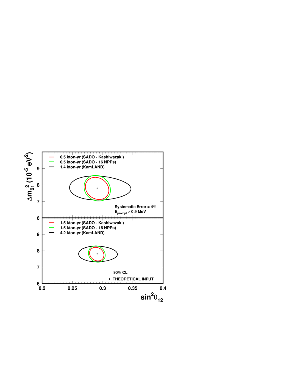
Figure 2: Comparison between the sensitivities at 90% CL for 2 DOF expected by KamLAND and SADO for runs with (about) equal number of events without oscillation. Neutrinos from all the 16 NPPs are taken into account for KamLAND whereas for SADO_single only Kashiwazaki-Kariwa NPP contribution was computed. The input values of mixing parameters are $\sin^{2}\theta_{12}=0.29$ and $\Delta m^{2}_{21}=7.9\times 10^{-5}$ eV². The numbers of events for 0.5 kt$\cdot$yr measurement at SADO_single and for 1.4 kt$\cdot$yr measurement at KamLAND will be about 1700. The systematic errors are assumed to be 4% in both detectors. Events with prompt energy ($E_{\text{prompt}}\equiv E_{\nu}$ - 0.8 MeV) greater than 0.9 MeV are used for both detectors. For a comparison, we also show the sensitivity, at 90% CL, expected for SADO_multi if the contributions of all 16 NPPs were included.

To answer this question, we present in Fig. 2 a comparison between the sensitivities to $\sin^{2}\theta_{12}$ attainable by SADO_single, SADO_multi located at 54 km, and KamLAND. This plot shows how accurately we can reproduce the input mixing parameters, $\sin^{2}\theta_{12}=0.29$ and $\Delta m^{2}_{21}=7.9\times 10^{-5}$ eV², which will be used throughout this paper.

For the purpose of comparison we have used for both, SADO and KamLAND, the same systematic error of 4% and the common energy threshold of $E_{\text{prompt}}=0.9$ MeV. We determined the exposure time of the each detector so that they receive (approximately) the same number of events without oscillation. By equalizing the number of events in this comparison, we aim to reveal how efficient the principle of tuning to the oscillation maximum for determining $\theta_{12}$ is. For SADO_multi and KamLAND we have included all 16 NPPs, while for SADO_single we have considered only contributions from the Kashiwazaki-Kariwa NPP. (The distances to the 16 NPPs from SADO and KamLAND are given in Table 4.)

In comparing KamLAND with SADO in this subsection, we have ignored the geo-neutrino contributions. Therefore, the comparison between SADO_multi and KamLAND is purely a comparison of the two different detector locations. The possible impact of geo-neutrinos on SADO will be described in Sec. III, and details of the analyzes in Secs. IV and V.

We discover in Fig. 2 the enormous power of SADO; the sensitivity attainable by SADO is better by a factor of $\simeq$ 2.5 than that of KamLAND for about three times longer operation in kt$\cdot$yr. We also notice that the sensitivities achievable by SADO_single and SADO_multi are comparable; the additional contribution from the other 15 reactors does not affect so much the $\theta_{12}$ determination. More quantitatively, we recognize from Fig. 2 that at 90% CL, the sensitivity attainable by SADO_single,multi corresponds to about 7% (5%) error in $\sin^{2}\theta_{12}$ for 0.5 kt$\cdot$yr (1.5 kt$\cdot$yr) measurement.

One may want to ask a further question. Namely, how long does KamLAND take to reach the same sensitivity as of SADO? (In fact, this is the question raised by one of the referees.) The answer to the question is in fact a surprising one: To achieve the same sensitivity of SADO_multi presented in the upper panel of Fig. 2, KamLAND would need more than 100 kt$\cdot$yr exposure. Whereas for the cases SADO_single shown in the upper panel and SADO_single,multi shown in the lower panel, KamLAND would not achieve the same sensitivities even in the limit of infinite statistics. Therefore, tuning the baseline distance is essential to achieve the ultimate sensitivity of 2% level for $\sin^{2}\theta_{12}$ determination.

We should mention that, for the lower value of $\Delta m^{2}_{21}=7.2\times 10^{-5}$ eV², preferred by the data KamLAND before KamLAND 2004 result, the optimal distance would have to be re-scaled to about 70 km (see Eq.(2)), resulting in a corresponding increase of a factor of two in running time in SADO to match the same sensitivity at higher $\Delta m^{2}_{21}$ achieved for 54 km.

II.4 $\sin^{2}{\theta_{12}}$ versus $\sin^{2}{2\theta_{12}}$

Though it is slightly off the main line of the discussion let us make some comments on usage of the variable in the plots we present in this paper. There have been various choices of variables for displaying allowed regions in $\theta_{12}$ - $\Delta m^{2}_{21}$ plane. They include, $\tan^{2}{\theta_{12}}$, $\sin^{2}{2\theta_{12}}$, and $\sin^{2}{\theta_{12}}$. We feel it important, if possible, to have a “standard choice” of the mixing variable to make comparison between different analysis easier. We choose $\sin^{2}{\theta_{12}}$ throughout this paper for reasons which are described below.

First of all, we now know that $\theta_{12}$ is in the first octant. Therefore, we have no more reasons to continue to use $\tan^{2}{\theta_{12}}$. Then, the question is which of $\sin^{2}{2\theta_{12}}$, or $\sin^{2}{\theta_{12}}$ is to be used. This is a difficult choice because both of them can be supported for good reasons from physics point of view. The solar neutrinos experience neutrino flavor transformation by different mechanisms at low and high energies. At low energies, it is essentially the vacuum oscillation effect that is dominant. At high energies the adiabatic MSW conversion effect takes over where the $\nu_{e}$ survival probability is approximately given by $\sin^{2}\theta_{12}$. Therefore, the natural variable at low and high energies are $\sin^{2}{2\theta_{12}}$, and $\sin^{2}{\theta_{12}}$, respectively, and they both have right to be chosen.

We use $\sin^{2}{\theta_{12}}$ in this paper because of two reasons. One is that $\sin^{2}{\theta_{12}}$ allows a direct physical interpretation as the probability of finding $\nu_{e}$ in the second mass eigenstate, as emphasized in parke-mena . The other one is that $\theta_{12}$ is relatively large, though not quite maximal. For large mixing angle $\theta$, $\sin^{2}{2\theta}$ is not a convenient variable because $\sin^{2}{2\theta}$ becomes insensitive to change in $\theta$. It can be simply understood by computing the Jacobian

$$\frac{\delta(\sin^{2}{2\theta})}{\delta(\sin^{2}\theta)}\simeq\frac{d\sin^{2}{2\theta}}{d\sin^{2}\theta}=4\cos{2\theta},$$ (3)

where $\delta(\sin^{2}\theta)$ and $\delta(\sin^{2}{2\theta})$ denote the error in $\sin^{2}\theta$ and $\sin^{2}{2\theta}$, respectively. It means that a large error obtained for $\sin^{2}\theta$ can be translated into a much more suppressed error for $\sin^{2}{2\theta}$ because of the small Jacobian at large $\theta\sim\pi/4$. Of course, the problem of disparity between errors estimated for these two variables in our case is much milder than that of atmospheric angle $\theta_{23}$ MSS .

III Requirements and possible obstacles for the precision measurement of $\theta_{12}$

In order to achieve the optimal sensitivity promised in the previous sections the following two requirements have to be met. They are: (i) experimental systematic error of 4% level, (ii) baseline distance of 50-70 km. We will discuss the requirement (i) and other related issues in this section. We calculate the optimal distance after setting up our analysis procedure in the next section.

III.1 Experimental systematic error

The key ingredients in the accurate measurement of $\theta_{12}$ in reactor experiments is the systematic error in the measurement. In this paper, we assume that there exists a dedicated front detector. It would be ideal if there already exists a near-far detector complex for reactor measurement of $\theta_{13}$ at less than 1-2 km from the principal reactor for SADO. Presence of the front detector is crucial to suppress the systematic errors for accurate measurement of $\theta_{12}$ because the various errors such as absolute flux and cross sections largely cancel between the front detector and SADO, in complete parallelism with the reactor $\theta_{13}$ measurement. See e.g., munich ; reactorCP for details on how and which errors can be canceled.

Since SADO cannot have structure exactly identical with the front detector, the systematic error may not be as small as $\sim$ 1%, the number expected to be reachable in reactor $\theta_{13}$ measurement reactor_white . We assume in our analysis, based on suekane , that the systematic error can be as small as 4% at SADO. This systematic error is supposed to include background from cosmic-ray events, assuming that the overburden is enough. Our claim that 4% systematic error may be in reach can be regarded as reasonable by recalling that the CHOOZ experiment CHOOZ already achieved the goal of the systematic error (1.5% for detection efficiency error) apart from the one due to flux normalization. Therefore, we think that the 4% is a conservative estimate and a smaller systematic error of $\simeq$2% may well be thinkable.

One of the consequence for the requirement of less than 4% systematic error is that we cannot rely on the event cut of the energy spectrum of prompt energy $E_{\text{prompt}}>2.6$ MeV to reject geophysical neutrino contamination, as done by the KamLAND group in their reactor neutrino analysis KamLAND ; KamLAND_new . Because of the uncertainty in the energy measurement it produces an additional $\simeq 2\%$ systematic error which makes over-all 4% systematic error difficult to achieve. Therefore, we must take all the events with prompt energy greater than 0.9 MeV. But it means that we have to deal with geophysical neutrinos in our analysis. It will be one of the most important issues in our sensitivity analysis in this paper.

III.2 Geophysical neutrinos; a brief review

Geo-neutrinos comes into play in our sensitivity analysis of $\theta_{12}$ because U (Th) decay series processes through six (four) $\beta$-decays, producing 6 (4) geo-neutrinos with energy $E_{\nu}\raise 1.29167pt\hbox{$\;<$\kern-7.5pt\raise-4.73611pt\hbox{$\sim\;$}}3.4$ MeV, or $E_{\text{prompt}}\raise 1.29167pt\hbox{$\;<$\kern-7.5pt\raise-4.73611pt\hbox{$\sim\;$}}2.4$ MeV. The threshold of $E_{\nu}^{\text{th}}=1.7$ MeV at SADO then implies that geo-neutrino events from U and Th decays can contaminate reactor neutrino events in our analysis.

Then, what are geo-neutrinos and do we know their properties? In the rest of this subsection, we briefly review what we know about geophysical neutrinos. The radioactive decay chains of radionuclides such as ⁴⁰K, ²³⁸U and ²³²Th inside the Earth produce not only heat but also electron antineutrinos. The fact that the radioactive heat flux and the geophysical neutrino flux are tightly linked was first pointed out by Eder eder in the sixties. Since then, the geo-neutrinos have been the subject of continuing interests geonu . Unfortunately, a quantitative accounting of the radioactive heat flux requires a detailed knowledge of the abundance distributions of these long-lived radioactive species inside the Earth. Our current knowledge of these abundance distributions is incomplete because of many reasons, for example, direct sampling is possible only at or near the surface and most of the Earth’s surface is inaccessible. Consequently, the radiogenic heat flux and therefore the geo-neutrino flux is largely model-dependent and its precise magnitude is unknown.

The presently estimated value for the global heat flux from the earth is 40 TW. It gives an upper bound on geo-neutrino flux from the interior of the earth. Heating from known radioactive sources in the surface layers (corresponding to 1/300 of the Earth’s total mass) is estimated to be already about 20 TW. Most geophysical models predict that the concentrations of radioactive sources will decrease rapidly with depth, but even small variations in these concentrations, for such a big mass as that of our planet, can greatly affect heat and geo-neutrino production.

We will treat geo-neutrinos flux as an additional parameter to be fit in our sensitivity analysis. To take proper care of its uncertainty we examine the two extreme cases of no geo-neutrino flux as an input and the maximum flux corresponding to global heat flux of 40 TW (the Fully Radiogenic Model). Fortunately, as we will see in the next two sections, the sensitivity on $\theta_{12}$ to be achieved by SADO is not disturbed in an essential way by the presence of geo-neutrinos provided that we choose appropriate baseline distances.

III.3 Uncertainty due to $\theta_{13}$

Uncertainty due to the unknown value of $\theta_{13}$ can be another source of the systematic error. It was shown in concha-pena that it can be regarded as an effective uncertainty in the flux normalization. Let us briefly review their argument. Since the vacuum neutrino oscillation is a good approximation for the reactor $\theta_{12}$ experiments, we can write down the electron antineutrino survival probability in a simple approximate form

$$P(\bar{\nu}_{e}\leftrightarrow\bar{\nu}_{e})=\sin^{4}\theta_{13}+\cos^{4}\theta_{13}\left[1-\sum_{i}f_{i}\sin^{2}2\theta_{12}\sin^{2}\left(\frac{\Delta m^{2}_{21}L_{i}}{4E_{\nu}}\right)\right],$$ (4)

where $E_{\nu}$ is the neutrino energy, $L_{i}$ is the distance to the detector from reactor $i$, and $f_{i}$ is the fraction of the total neutrino flux which comes from reactor $i$. Thus, nonzero $\theta_{13}$ effectively acts as an uncertainty in the flux normalization of less than 8%, giving the CHOOZ constraint $\sin^{2}2\theta_{13}<0.15$ at 90% CL bari_update .

This uncertainty in the flux normalization cannot be canceled by measurement at the front detector. Therefore, $\theta_{13}$ has to be determined by an independent measurement. But the experimental determination of $\theta_{13}$ should always come with errors, $\delta(\sin^{2}{2\theta_{13}})$. It will produce an effective uncertainty in the probability by the amount

$$\delta(\cos^{4}\theta_{13})\simeq\left|\frac{d\cos^{4}\theta_{13}}{d(\sin^{2}{2\theta_{13}})}\right|\delta(\sin^{2}{2\theta_{13}})\simeq\frac{1+\tan^{2}{\theta_{13}}}{2}\delta(\sin^{2}{2\theta_{13}}),$$ (5)

for a given experimental error $\delta(\sin^{2}{2\theta_{13}})$ of measurement. If we take the estimation in MSYIS for reactor $\theta_{13}$ experiment, $\delta(\sin^{2}{2\theta_{13}})\simeq 0.012$ (0.02 at 90% CL) almost independently of the true values of $\sin^{2}{2\theta_{13}}$. Therefore, we expect an uncertainty of $\simeq 0.6$% level in the probability and hence in $\sin^{2}{2\theta_{12}}$. It may be translated, by using (3), into an uncertainty on $\sin^{2}{\theta_{12}}$ of about 0.4% at the current best fit of $\theta_{12}$.

Thus, the error of $\theta_{13}$, once it is measured by reactor experiments, adds only $\simeq$ 0.4% to the uncertainty on $\sin^{2}{\theta_{12}}$. Though it does not pose any serious problem, more precise measurement of $\theta_{13}$ either by LBL high-intensity superbeam experiments with both neutrino and antineutrino modes JPARC ; NuMI ; SPL , or by high statistics reactor experiments reactor_white or even by neutrino factory nufact is highly welcome.

We assume in the rest of this paper vanishing $\theta_{13}$ for simplicity. Assuming $\theta_{13}$ is determined with error much smaller than 1% the effect of nonzero $\theta_{13}$ effectively acts as smaller $\bar{\nu}_{e}$ flux by a factor of $\cos^{4}{\theta_{13}}$. For example, if $\theta_{13}$ is on the edge of the above CHOOZ bound, $\cos^{4}{\theta_{13}}=0.92$, we need 9% longer running time to obtain the same sensitivities as presented in the later sections.

IV Analysis procedure and estimation of the optimal distances

In this section, we first make a rough description of our analysis procedure, and then estimate the optimal distances for reactor $\theta_{12}$ experiments. For more details of the analysis procedure, we refer the readers to Appendix B.

IV.1 Analysis procedure in brief

We follow our previous papers NTZ02 ; Nunokawa:2003dd in calculating the number of neutrino events expected from reactors as well as from Th and U radioactive decays in the Earth at a liquid scintillator detector, SADO. We will give our results in terms of $\text{GW}_{\text{th}}\cdot\text{kt}\cdot\text{yr}$. Notice that 10 $\text{GW}_{\text{th}}\cdot\text{kt}\cdot\text{yr }$ is approximately equivalent to 1 year exposure of 0.5 kt detector at 54 km away from Kashiwazaki-Kariwa NPP operating at 80% efficiency.

The total number of events from a single NPP for an exposure of 1 $\text{GW}_{\text{th}}\cdot\text{kt}\cdot\text{yr }$, for the used threshold energy is estimated to be,

$$N^{\text{reac}}_{\text{total}}(E_{\text{prompt}}>0.9{\text{ MeV}})=\displaystyle\left\{\begin{array}[]{c}141\\ 46\end{array}\right\}\times\left[\frac{L}{54\ \text{km}}\right]^{-2}\ \ [\text{GW}_{\text{th}}\cdot\text{kt}\cdot\text{yr }]^{-1},$$

where the upper (lower) value corresponds to no oscillation (oscillation at the input values used in this work). $\text{GW}_{\text{th}}$ is defined to be the thermal power actually generated, which should not be confused with the maximal thermal power of a given NPP.

The total number of events from geo-neutrinos expected from the Fully Radiogenic Model geonu at Mt. Komagatake is

$$N^{\text{geo}}_{\text{total}}(E_{\text{prompt}}>0.9{\text{ MeV}})=49\ [\text{kt}\cdot\text{yr }]^{-1}.$$ (6)

Since we currently do not know the U and Th geo-neutrino fluxes we consider two extreme cases: (i) zero geo-neutrino input and (ii) geo-neutrino input flux from U and Th computed assuming that the radiogenic production accounts for the total Earth heat flow of 40 TW (input from the Fully Radiogenic Model). They represent two extremes of the input geo-neutrino flux between zero and 3$\times 10^{7}$ cm^-2 s^-1 at the position of the detector, and one would expect the real situation to be somewhere between these two numbers. Note that even if we assume zero geo-neutrino input, we allow non-zero geo-neutrino flux as an output in our fit which can confuse reactor neutrinos. Since the ratio of U to Th contributions is rather well defined and common in varying models, we assume in our analysis that their relative contribution is held fixed while we treat an over-all absolute normalization as a free parameter. The Th contribution is assumed to be 83% of the total geo-neutrino flux geonu . This procedure should be (and will be) tested by future KamLAND data which includes $E_{\text{prompt}}<2.6$ MeV. Of course, having the additional free parameter in general makes the sensitivity on $\theta_{12}$ worse.

We use the following definition of the $\chi^{2}$ function as

$$\chi^{2}(\sin^{2}\theta_{12},\Delta m^{2}_{21},\phi_{\text{U}})=\displaystyle\sum_{i=1}^{17}\frac{\left[N_{i}^{\text{exp}}-N_{i}^{\text{theo}}(\sin^{2}\theta_{12},\Delta m^{2}_{21},\phi_{\text{U}})\right]^{2}}{\sigma_{i}^{2}},$$ (7)

where $\sigma_{i}=\sqrt{N_{i}^{\text{exp}}+(0.04\,N_{i}^{\text{exp}})^{2}}$ is the statistical plus systematic uncertainty in the number of events in the $i$-th bin; $N_{i}^{\text{theo}}$ is the theoretical expected number of events as functions of mixing parameters as well as $\phi_{\text{U}}$, the total geo-neutrino flux from U, to be fitted, calculated as explained in the Appendix B; $N_{i}^{\text{exp}}\equiv N_{i}^{\text{theo}}(\sin^{2}\theta_{12}(\text{input}),\Delta m^{2}_{21}(\text{input}),\phi_{\text{U}}(\text{input}))$ is the simulated expected number of events at the detector for the input values of the mixing parameters as well as geo-neutrino flux, assumed in this paper, i.e., $\sin^{2}\theta_{12}({\text{input}})=0.29$ and $\Delta m^{2}_{21}({\text{input}})=7.9\times 10^{-5}$ eV² and the geo-neutrino input, $\phi_{\text{U}}(\text{input})$, will be either zero or equal to what is expected if the radiogenic contribution to the terrestrial heat is to be explained by the Fully Radiogenic Model. The crustal contribution was estimated as in Ref. Nunokawa:2003dd but for a detector located at Mt. Komagatake in Niigata prefecture, Japan.

Using the $\chi^{2}$ function we compute the region in the $(\sin^{2}\theta_{12},\Delta m^{2}_{21})$ space allowed by SADO spectrum data at 68.27%, 90%, 95%, 99% and 99.73% CL for a given $\text{GW}_{\text{th}}\cdot$kt$\cdot$yr exposure.

IV.2 Optimal baseline distance

We have discussed in Sec. II that it is the key for a precise measurement of $\theta_{12}$ measurement to choose the baseline distance which corresponds to the oscillation maximum. To seek ultimate sensitivity on $\theta_{12}$, however, we must first elaborate this point.

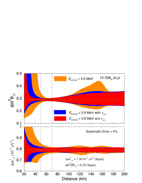
Figure 3: Achievable precision of the determination of the oscillation parameters at 68.27% CL for 1 DOF as a function of the detector distance from the Kashiwazaki-Kariwa NPP for 10 GW${}_{\text{th}}\cdot$kt$\cdot$yr exposure and energy thresholds of $0.9$ and 2.6 MeV. The horizontal dashed lines indicate the input values of the mixing parameters. The geo-neutrino contribution was calculated as predicted by the Fully Radiogenic Model. For the lower energy threshold the $\chi^{2}$ was minimized allowing the total geo-neutrino flux to vary from 0 to 3$\times 10^{7}$ cm^-2 s^-1. We have used the input values of the mixing parameters corresponding to $\sin^{2}\theta_{12}=0.29$ and $\Delta m^{2}_{21}=7.9\times 10^{-5}$ eV². The vertical dashed lines indicate the optimal range for SADO detector.

We show, in the upper and the lower panels in Fig. 3, the accuracy of determination of $\sin^{2}\theta_{12}$ and $\Delta m^{2}_{21}$, respectively, as a function of $L$ expected by 10 GW${}_{\text{th}}\cdot$kt$\cdot$yr exposure computed by the minimization of the $\chi^{2}$ function that is defined in Sec. III. The results for two different energy thresholds, $0.9$ and $2.6$ MeV, are presented for the purpose of comparison. For the case $E_{\text{prompt}}>0.9$ MeV, we show two curves for sensitivity with and without geo-neutrino background contribution. We note that both $\Delta m^{2}_{21}$ and $\theta_{12}$ are left free and marginalized in the analysis to obtain the sensitivity of $\sin^{2}\theta_{12}$ and $\Delta m^{2}_{21}$, as presented respectively in the upper and the lower panels in Fig. 3.

We see that when the analysis threshold is higher the best place to put a detector, in order to achieve greater sensitivity to $\theta_{12}$, is at around $L\simeq L_{\text{OM}}=63$ km, in agreement with our rough expectation. On the other hand, when the threshold is lower, it is preferable to choose values of $L$ 10-25% smaller than $L_{\text{OM}}$.

It is remarkable that if there were no geo-neutrinos the baseline distance as short as 40 km could be suitable. Even when we take them into account, the optimal distance ranges between 50 and 70 km which is still a relatively wide range. We will see below (Sec. V) that even at 70 km, the longest end of the distance range, the sensitivity is worse only by about 15% or so than SADO at 54 km. This point is very important and encouraging for people who try to design reactor $\theta_{12}$ experiments because a wide band of radii between 50 and 70 km around a particular reactor NPP can serve as a potential location for the experiment.

The reason why the effect of geo-neutrinos is larger at shorter distances is as follows. As $L$ gets shorter the region where oscillation effect is sizable moves to lower energies. Then, for $L\raise 1.29167pt\hbox{$\;<$\kern-7.5pt\raise-4.73611pt\hbox{$\sim\;$}}50$ km it starts to invade the region of $E_{\nu}<3.4$ MeV where geo-neutrinos live.

An interesting behavior of the error on $\sin^{2}\theta_{12}$ for the $2.6$ MeV threshold, rapidly increasing with $L$ from about 80 to 150 km and decreasing again from 150 to about 170 km, can be explained as follows. The maximal sensitivity, reached at about 60 km, corresponds to the first oscillation maximum at the peak of the event distribution. As $L$ increases this first oscillation maximum moves to higher energies, finally going out of the reactor neutrino energy spectrum. When the second oscillation maximum passes the $2.6$ MeV threshold, at about 150 km, it improves the $\sin^{2}\theta_{12}$ determination causing the partial recovery of precision.

In the lower panel of Fig. 3 we appreciate the weak dependence on $L$ of the accuracy in the determination of $\Delta m^{2}_{21}$ for $L\raise 1.29167pt\hbox{$\;>$\kern-7.5pt\raise-4.73611pt\hbox{$\sim\;$}}$ 50 km. We will see in Sec. VII (Table 3) that SADO does improve the sensitivity of $\Delta m^{2}_{21}$ determination over the KamLAND’s though not to the extent that occurs for $\theta_{12}$.

It is interesting to clarify the difference between our case and that of the experimental set up of the next generation LBL accelerator neutrino experiments JPARC ; NuMI ; SPL . In particular, in the JPARC-SK experiment, the accuracy of determination of $\sin^{2}{2\theta_{23}}$ is expected to reach down to $\simeq$ 1% at 90% CL JPARC . In this experiment, where $L$ is already fixed, the best sensitivity for the angle determination is obtained when the experiment is tuned to the energy which corresponds to the first oscillation maximum. The spectrum of an off-axis beam is nearly monochromatic. On the other hand, in the reactor experiment we are considering, the energy spectrum is given and is quite broad and hence nearly maximal sensitivity to the mixing angle can be achieved in a range of values of $L$.

V How accurate is the reactor measurement of $\theta_{12}$?

In this section, we give a quantitative estimate of the sensitivity which can be achievable in a dedicated reactor measurement of $\theta_{12}$.

V.1 Analysis of sensitivity on $\theta_{12}$: SADO at 54 km

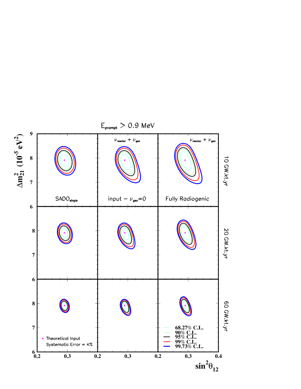
Figure 4: Precision of the determination of the oscillation parameters by SADO${}_{\text{single}}$, a detector at 54 km from the Kashiwazaki-Kariwa NPP, for exposures of 10 $\text{GW}_{\text{th}}\cdot$kt$\cdot$yr (upper panels), 20 $\text{GW}_{\text{th}}\cdot$kt$\cdot$yr (middle panels) and 60 $\text{GW}_{\text{th}}\cdot$kt$\cdot$yr (lower panels). Left and middle panels have no geo-neutrino input, but in the middle panels geo-neutrinos were however taken into account in the fit. Right panels were calculated for geo-neutrino input according to the Fully Radiogenic Model. The confidence level regions were computed for 2 DOF.

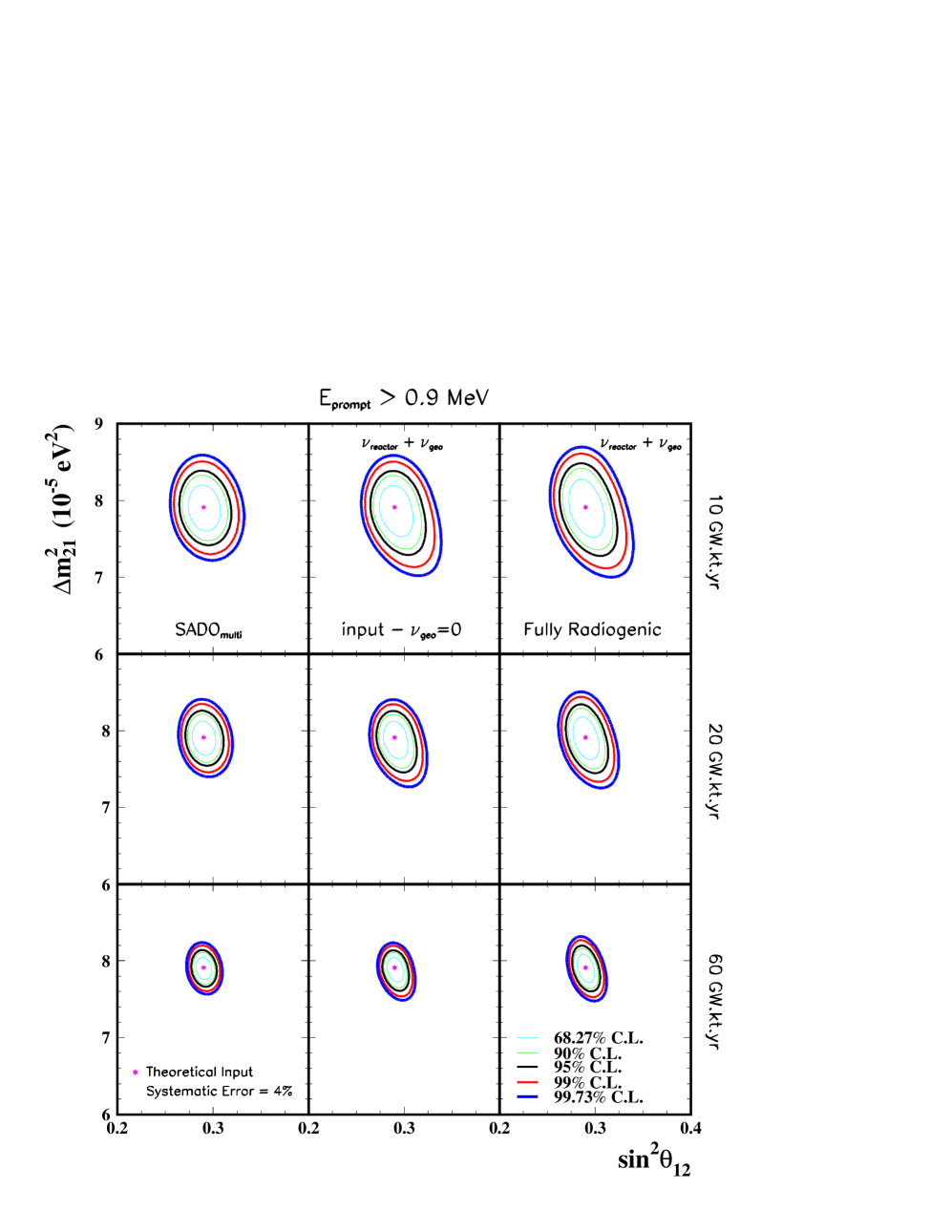
Figure 5: Same as Fig. 4 but for SADO${}_{\text{multi}}$ with all 16 reactor NPPs included.

We show in Fig. 4 how precisely the mixing parameters can be determined by SADO${}_{\text{single}}$, assuming that only the Kashiwazaki-Kariwa NPP will be contributing to the neutrino flux at the detector site, for exposures of 10 $\text{GW}_{\text{th}}\cdot$kt$\cdot$yr (upper panels), 20 $\text{GW}_{\text{th}}\cdot$kt$\cdot$yr (middle panels) and 60 $\text{GW}_{\text{th}}\cdot$kt$\cdot$yr (lower panels). In the left panels, geo-neutrinos were not considered, in the middle panels, we have set the geo-neutrino flux input to be zero but allowed the flux to be fitted to vary freely in the $\chi^{2}$ fit. In the right panels, we have calculated the geo-neutrino input according to the Fully Radiogenic Model and allowed the flux to be fitted to vary freely in the $\chi^{2}$ fit.

In Fig. 5 we provide the same information as in Fig. 4 but for SADO${}_{\text{multi}}$ which includes the contributions of all the 16 reactor NPPs in Japan. We note that by taking into account the contributions from the other 15 reactor NPPs, the accuracy of determination of $\sin^{2}\theta_{12}$ becomes slightly worse. The error on $\Delta m^{2}_{21}$ also slightly increases.

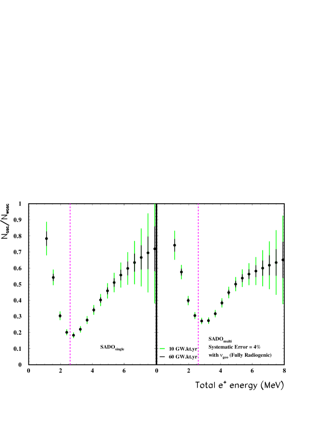
Figure 6: Spectral distortion expected as a function of the $e^{+}$ prompt energy for SADO${}_{\text{single}}$ (left panel) and SADO${}_{\text{multi}}$ (right panel). Each ratio is represented as a point with the corresponding error bar for a given exposure (10 and 60 $\text{GW}_{\text{th}}\cdot$kt$\cdot$yr). The number of oscillation events at each bin was calculated for the input values $\sin^{2}\theta_{12}=0.29$ and $\Delta m^{2}_{21}=7.9\times 10^{-5}$ eV². The dashed line indicates the maximal energy for geo-neutrinos. Geo-neutrino contribution from the Fully Radiogenic Model was included.

The inclusion of geo-neutrinos does not influence very much the sensitivity to $\sin^{2}\theta_{12}$ as can be seen in Figs. 4 and 5. This is because we have chosen a distance such that the position of the dip is far enough from the geo-neutrino energy region. This can be visualized in Fig. 6, where we present the normalized expected energy spectra at SADO${}_{\text{single}}$ (left panel) and SADO${}_{\text{multi}}$ (right panel) for exposures of 10 and 60 $\text{GW}_{\text{th}}\cdot$kt$\cdot$yr. The impact of the inclusion of the 15 NPPs is to modify somewhat the shape of the spectrum.

On the other hand, the sensitivity to $\Delta m^{2}_{21}$ is slightly more affected by the inclusion of the geo-neutrino background. This is because in $\Delta m^{2}_{21}$ determination, it is important to observe the shape of the spectrum in the entire energy range making it more sensitive to the geo-neutrino contributions in the lower energy bins. At this point it is also instructive to look at Fig. 7, where we show the $\Delta\chi^{2}=\chi^{2}$ behavior as a function of $\sin^{2}\theta_{12}$ and $\Delta m^{2}_{21}$ for 10, 20 and 60 $\text{GW}_{\text{th}}\cdot$kt$\cdot$yr exposure, all 16 NPPs considered.

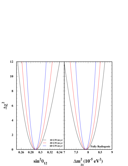
Figure 7: $\Delta\chi^{2}$ as a function of the oscillation parameters around the minimum for 10, 20 and 60 $\text{GW}_{\text{th}}\cdot$kt$\cdot$yr exposure. All 16 reactor NPPs were included in the calculation and the prompt energy threshold used was 0.9 MeV. Geo-neutrino contribution from the Fully Radiogenic Model was included.

Table 1: The expected sensitivity to the solar mixing angle at SADO${}_{{\text{single}}}$ (SADO${}_{{\text{multi}}}$) at 1 $\sigma$ (68.27%) and 3 $\sigma$ (99.73%) CL for 1 DOF obtained for SADO at Mt. Komagatake (54 km, the upper rows) and Sado gold mine (71 km, the lower rows). They are calculated with the prompt energy threshold of 0.9 MeV and with the background effect of geo-neutrinos from Fully Radiogenic Model. The numbers for SADO${}_{{\text{multi}}}$ are computed for both detectors by using position-dependent contributions from all the 16 NPPs.

exposure	$\sin^{2}\theta_{12}$ [68.27% CL]	$\sin^{2}\theta_{12}$ [99.73% CL]
54 km
10 $\text{GW}_{\text{th}}\cdot$kt$\cdot$yr	$0.29^{+0.014}_{-0.013}$ ($0.29^{+0.015}_{-0.014}$)	$0.29^{+0.040}_{-0.031}$ ($0.29^{+0.042}_{-0.033}$)
20 $\text{GW}_{\text{th}}\cdot$kt$\cdot$yr	$0.29^{+0.010}_{-0.010}$ ($0.29^{+0.011}_{-0.011}$)	$0.29^{+0.028}_{-0.023}$ ($0.29^{+0.030}_{-0.025}$)
60 $\text{GW}_{\text{th}}\cdot$kt$\cdot$yr	$0.29^{+0.006}_{-0.006}$ ($0.29^{+0.007}_{-0.007}$)	$0.29^{+0.017}_{-0.015}$ ($0.29^{+0.019}_{-0.017}$)
71 km
10 $\text{GW}_{\text{th}}\cdot$kt$\cdot$yr	$0.29^{+0.016}_{-0.015}$ ($0.29^{+0.019}_{-0.017}$)	$0.29^{+0.045}_{-0.037}$ ($0.29^{+0.052}_{-0.040}$)
20 $\text{GW}_{\text{th}}\cdot$kt$\cdot$yr	$0.29^{+0.012}_{-0.011}$ ($0.29^{+0.013}_{-0.012}$)	$0.29^{+0.031}_{-0.027}$ ($0.29^{+0.036}_{-0.030}$)
60 $\text{GW}_{\text{th}}\cdot$kt$\cdot$yr	$0.29^{+0.007}_{-0.007}$ ($0.29^{+0.008}_{-0.008}$)	$0.29^{+0.018}_{-0.016}$ ($0.29^{+0.022}_{-0.020}$)

We summarize in Table 1 the accuracy of determination of the mixing angle $\theta_{12}$ which can be achieved by SADO${}_{\text{single}}$ and SADO${}_{\text{multi}}$ for these three exposures. We use the prompt energy threshold of 0.9 MeV and take into account the background effect of geo-neutrinos expected by the Fully Radiogenic Model, the most conservative estimate. We have investigated the dependence of this accuracy on the input value of $\Delta m^{2}_{21}$ by varying it in the range $\Delta m^{2}_{21}=(7-9)\times 10^{-5}{\text{ eV}^{2}}$. We have discovered the accuracy becomes somewhat worse, at most by 30%, if the input value is smaller than the current best fit one due to geo-neutrinos, whereas for higher values there is practically no change.

In Table 1, we also present for comparison the results of our analysis for a detector placed at Sado island, about 71 km away from the Kashiwazaki-Kariwa NPP. As one can anticipate from Fig. 3 the sensitivity at 71 km is worse than that of SADO at 54 km but only by 15-20%. Thus, SADO at the Sado island is still a valid option for the reactor $\theta_{12}$ experiment.

VI Stability of the results against changes in statistical procedure

We have shown in the previous sections that the sensitivity for $\theta_{12}$ attainable by SADO with a modest requirement of $\simeq$ 4% systematic error is extremely good, which is competitive to all the methods so far proposed. In this section we confirm the stability of the results by using different definitions of $\chi^{2}$. While we believe that our statistical method and the treatment of errors based on $\chi^{2}$ defined in Eq. (7) is reasonable and a standard one, it is nice if we can explicitly verify that our results are stable against changes in the statistical procedure.

For this purpose, we examine the following two possible choices of $\chi^{2}$. The first one, which is frequently used in various statistical analyzes of data, reads

$$\chi^{2}_{\text{corr}}=\min_{\text{$\alpha$}}\sum_{i=1}^{17}\frac{(N^{\rm exp}_{i}-\alpha\,N^{\rm theo}_{i})^{2}}{N^{\rm exp}_{i}}+\frac{(\alpha-1)^{2}}{\sigma^{2}_{\rm syst}},$$ (8)

where $N^{\rm exp}_{i}$ and $N^{\rm theo}_{i}$ are defined in the same way as in our $\chi^{2}$ definition in (7). The $\chi^{2}$ was used, for example, in the KamLAND analysis in Ref. concha04 . We take, as in our analysis, $\sigma_{\rm syst}=4$%. As we will see below, this choice of $\chi^{2}$ leads to even higher sensitivity of $\theta_{12}$ measurement at SADO. It is not surprising to obtain such result because the systematic uncertainty affects all bins simultaneously for $\chi^{2}$ in (8), whereas it can fluctuate bin-by-bin with our definition of $\chi^{2}$ in Eq. (7).

Our second choice of $\chi^{2}$ is the one used for the analysis in reactor $\theta_{13}$ measurement munich . In such experiments we compare yields at identical near and far detectors and a large portion of the systematic errors cancels out in such a setting. Therefore, the statistical treatment involves the errors which have different characteristics, (un-)correlated between near and far detectors, and between bins. Following munich ; reactorCP , we consider four types of systematic errors: $\sigma_{\rm DB}$, $\sigma_{\rm Db}$, $\sigma_{\rm dB}$, and $\sigma_{\rm db}$. The subscript D (d) represents the fact that the error is correlated (uncorrelated) between detectors. The subscript B (b) represents that the error is correlated (uncorrelated) among bins. The definition of $\chi^{2}$ is

$$\chi^{2}_{\text{nf}} \equiv \min_{\text{$\alpha$'s}}\sum_{a=f,n}\left[\sum_{i=1}^{17}\left\{\frac{\left(N^{\rm theo}_{ai}-(1+\alpha_{i}+\alpha_{a}+\alpha)N^{\rm exp}_{ai}\right)^{2}}{N^{\rm exp}_{ai}+\sigma_{\rm db}^{2}(N^{\rm exp}_{ai})^{2}}+\frac{\alpha_{i}^{2}}{\sigma_{\rm Db}^{2}}\right\}+\frac{\alpha_{a}^{2}}{\sigma_{\rm dB}^{2}}\right]+\frac{\alpha^{2}}{\sigma_{\rm DB}^{2}},$$ (9)

where $N_{ai}^{\rm theo}$ represents the theoretical number of events at the near ($a=n$) or far ($a=f$) detector within the $i$-th bin. Again, $N_{ai}^{\rm exp}$ is defined as the number of signal event calculated with the best-fit parameters of the “experimental data”. See reactorCP for more details.

To simulate the reactor $\theta_{13}$ measurement with sensitivity up to $\simeq$ 1% which is, very roughly speaking, equivalent to sensitivity up to $\sin^{2}2\theta_{13}=0.01$ for a long enough exposure (systematics dominated measurement), the following numbers have been taken for these errors reactorCP ; $\sigma_{\rm DB}=\sigma_{\rm Db}=2.5$% and $\sigma_{\rm dB}=\sigma_{\rm db}=0.5$%. To simulate the systematic error of $\simeq$ 4% at SADO we tentatively multiply by 4 all these errors. That is, we take $\sigma_{\rm DB}=\sigma_{\rm Db}=10$% and $\sigma_{\rm dB}=\sigma_{\rm db}=2$% in our analysis for SADO. We also examine the optimistic case of systematic error of $\simeq$ 2% at SADO, considering the possibility that the systematic error can be improved. The errors for this case are taken as 1/2 of the 4% case. We have confirmed in the case of $\theta_{13}$ measurement that the error twice (four times) larger than that of reactorCP leads to the sensitivity approximately equal to $\sin^{2}2\theta_{13}=0.02$ (0.04) for long enough exposure.

Since the front detector and SADO will be different in volume, assuming equal errors for both detector is nothing more than a crude approximation. But, we feel that it gives a reasonable framework to check the stability of our statistical treatment.

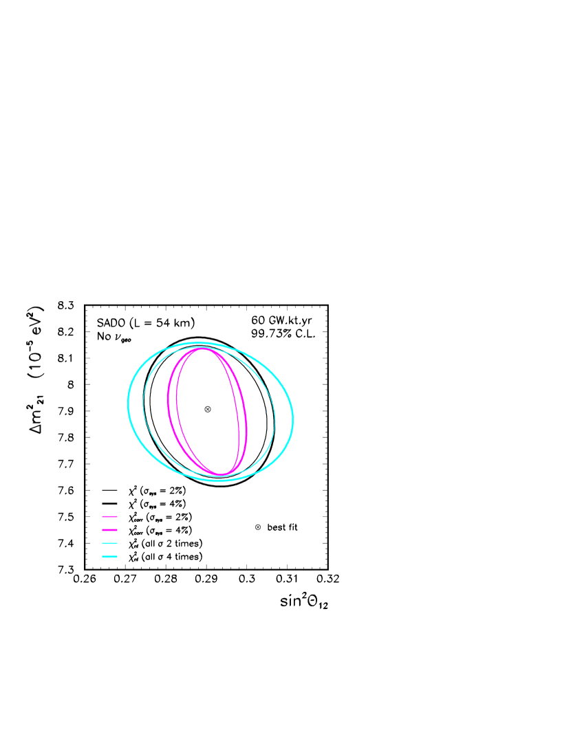
Figure 8: Regions allowed at 99.73% CL for 60 $\text{GW}_{\text{th}}\cdot$kt$\cdot$yr exposure, determined by using three different $\chi^{2}$ definitions: the definition used throughout this paper (Eq. (7)), $\chi^{2}_{\rm corr}$ defined in Eq. (8) and $\chi^{2}_{\rm nf}$ defined in Eq. (9). The contours with $\chi^{2}$ defined above are, in order, the middle (black line), the thinnest (red) and the thickest (blue) ones in widths.

In Fig. 8 we show the result of our analysis with three different definitions of $\chi^{2}$, (8) and (9) defined above, and the one given in (7) that is adopted in our analysis. We observe that our result obtained in the previous section by using the $\chi^{2}$ in (7) lies between the results of the analysis with two different $\chi^{2}$, in (8) and (9). It is expected that the result with $\chi^{2}$ in (8) gives tighter constraint on the oscillation parameters because the way how the systematic error is treated only allows fluctuation of the absolute normalization, not bin-by-bin independent fluctuations, and it is harder to mimic spectral shape distortion. We do not have any good physics intuition on what would be the result for the choice of $\chi^{2}$, in (9), but it turns out that the sensitivity is a little worse than our estimate with (7). Nonetheless, the difference between the results obtained by using three different definitions of $\chi^{2}$ is not significant. Hence, we conclude that our estimate of the sensitivity of $\theta_{12}$ determination at SADO is stable under change of statistical treatment.

VII Comparison of sensitivities of reactor $\theta_{12}$ measurement with other methods

In this section, we compare the sensitivity calculated in Sec. V for a reactor measurement of $\theta_{12}$ at SADO with the ones expected by other methods, in particular the solar neutrino experiments. We assume CPT symmetry in the discussions in this subsection.

To date the most accurate determination of $\theta_{12}$ can be accomplished by combining all the solar neutrino experiments and KamLAND data sno_salt . According to Table 2 of Ref. concha04 , the current solar neutrino data together with KamLAND result can be used to determine $\sin^{2}{\theta_{12}}$ with about $\sim 8$% precision at 68.27% CL for 1 DOF. From the Table 3 of Ref. bahcall-pena , one expects that this precision will not be significantly reduced even if one combines with future KamLAND data corresponding to 3 years of exposure.

It is expected that if future solar neutrino experiments can detect $pp$ neutrinos selectively, they would give the best sensitivity to $\theta_{12}$ determination. Assuming the most optimistic error of 1% for pp neutrino measurement and by combining with the other solar neutrino experiments as well as with 3 years running of KamLAND, one expects, from Table 8 of Ref. bahcall-pena , that it is possible to measure $\sin^{2}\theta_{12}$ with uncertainty of $\sim 4$% at 68.27% CL for 1 DOF. Despite the fact that this result is obtained with the previous best fit value of $\Delta m^{2}_{21}$ ($\sim 7\times 10^{-5}$ eV²) it appears to be safe to assume that it will remain almost unchanged because the final precision of $\theta_{12}$ is essentially determined by the solar neutrino data.

The sensitivities expected by a reactor neutrino experiment calculated in the previous subsection should be compared with the precision obtained by all solar + KamLAND experiments mentioned above. This is done in Table 2 from which one can see that SADO${}_{\text{single,multi}}$ with exposure longer than 20 $\text{GW}_{\text{th}}\cdot$kt$\cdot$yr, can determine $\theta_{12}$ better than all other observations combined. We want to mention that Gd-loaded Super-Kamiokande GdSK cannot compete with the SADO’s sensitivity on $\theta_{12}$ choubey . Even after combining with the solar data the error 15% on $\sin^{2}\theta_{12}$ at 99% CL for 3 years operation is larger than SADO’s 12% at 99.97% CL for its 10 $\text{GW}_{\text{th}}\cdot$kt$\cdot$yr ($\simeq 0.5$ kt$\cdot$yr at SADO) exposure. It should be stressed that SADO alone can achieve such great precision without being combined with any other experiments, assuming that $\theta_{13}$ is measured with reasonable precision. Therefore, we conclude that a reactor measurement can supersede other methods for precise measurement of $\theta_{12}$ if the experimental systematic error of 4% is realized.

Table 2: Comparisons of fractional errors of the experimentally determined mixing angle, $\delta s^{2}_{12}/s^{2}_{12}\equiv\delta(\sin^{2}\theta_{12})/\sin^{2}\theta_{12}$, by current and future solar neutrino experiments and KamLAND (KL), obtained from Tables 3 and 8 of Ref. bahcall-pena , versus that by SADO${}_{\text{single}}$ (SADO${}_{\text{multi}}$) obtained in this work at 68.27% and 99.73% CL for 1 DOF.

Experiments	$\delta s^{2}_{12}/s^{2}_{12}$ at 68.27% CL	$\delta s^{2}_{12}/s^{2}_{12}$ at 99.73% CL
Solar+ KL (present)	$8$ %	$26$ %
Solar+ KL (3 yr)	$7$ %	$20$ %
Solar+ KL (3 yr) + pp (1%)	$4$ %	$11$ %
54 km
SADO for 10 $\text{GW}_{\text{th}}\cdot$kt$\cdot$yr	4.6 %   (5.0 %)	12.2 %  (12.9 %)
SADO for 20 $\text{GW}_{\text{th}}\cdot$kt$\cdot$yr	3.4 %   (3.8 %)	8.8 %   (9.5 %)
SADO for 60 $\text{GW}_{\text{th}}\cdot$kt$\cdot$yr	2.1 %   (2.4 %)	5.5 %   (6.2 %)

Although our main concern in this paper is a precise determination of $\theta_{12}$ let us briefly discuss the sensitivity of SADO on $\Delta m^{2}_{21}$ and its comparison with the one by other methods. In Table 3 we present the expected sensitivity to $\Delta m^{2}_{21}$ at SADO${}_{{\text{single}}}$ (SADO${}_{{\text{multi}}}$) at 1 $\sigma$ (68.27%) and 3 $\sigma$ (99.73%) CL for 1 DOF, obtained with the prompt energy threshold of 0.9 MeV and with the background effect of geo-neutrinos from Fully Radiogenic Model. The present KamLAND data together with all the solar neutrino data already achieved 14% error at 3$\sigma$ CL on $\Delta m^{2}_{21}$ determination. As one can see from Table 3 (and Fig. 5), SADO${}_{{\text{single}}}$ (SADO${}_{{\text{multi}}}$) will be able to reduce the error down to 4.3% (4.6%) at 3$\sigma$ CL for 60 $\text{GW}_{\text{th}}\cdot$kt$\cdot$yr operation. The error is smaller by a factor of 2 than that expected for the combined analysis of the future solar neutrino data and 3 years operation of KamLAND found in Fig. 6 of Ref.bahcall-pena . Nevertheless, it is still greater than the error of about 2.8% at 3$\sigma$ CL achievable by Gd-loaded Super-Kamiokande for its three years operation choubey .

Table 3: The expected sensitivity to the $\Delta m^{2}_{21}$ at SADO${}_{{\text{single}}}$ (SADO${}_{{\text{multi}}}$) at 1 $\sigma$ (68.27%) and 3 $\sigma$ (99.73%) CL for 1 DOF, obtained with the prompt energy threshold of 0.9 MeV and with the background effect of geo-neutrinos from Fully Radiogenic Model.

54 km
exposure	$\Delta m^{2}_{12}\times 10^{5}$ eV2 [68.27% CL]	$\Delta m^{2}_{12}\times 10^{5}$ eV2 [99.73% CL]
10 $\text{GW}_{\text{th}}\cdot$kt$\cdot$yr	$7.90^{+0.28}_{-0.30}$ ($7.90^{+0.30}_{-0.30}$)	$7.90^{+0.63}_{-0.83}$ ($7.90^{+0.70}_{-0.78}$)
20 $\text{GW}_{\text{th}}\cdot$kt$\cdot$yr	$7.90^{+0.21}_{-0.21}$ ($7.90^{+0.21}_{-0.21}$)	$7.90^{+0.48}_{-0.57}$ ($7.90^{+0.54}_{-0.56}$)
60 $\text{GW}_{\text{th}}\cdot$kt$\cdot$yr	$7.90^{+0.13}_{-0.14}$ ($7.90^{+0.15}_{-0.14}$)	$7.90^{+0.33}_{-0.35}$ ($7.90^{+0.36}_{-0.36}$)

VIII Physics implications of accurate measurement of $\theta_{12}$

There exist a variety of physics implications available when accurate measurement of $\theta_{12}$ is carried out. Here, we describe only a part of them. Of course, $\theta_{12}$ is one of the fundamental parameters of particle physics and its precise determination is by itself clearly important, as already discussed in Introduction. It may be appropriate to add a remark in this context. Namely, the determination of $\sin^{2}\theta_{12}$ to 2% level is comparable in accuracy to that of the Cabibbo angle, which is about 1.4% at this moment PDG . Therefore, SADO can open the new era in which we can enjoy balanced knowledge of lepton and quark mixings.

In the rest of this section, we focus on points which may have greater impact on wider areas of research, including symmetry tests, solar astrophysics and the earth science. Let us start by discussing implications to solar astrophysics, and then move on to the other topics. We assume, apart from Sec.VIII D, the CPT invariance in our discussions.

VIII.1 Observational solar astrophysics

One of the purposes of the future solar neutrino experiments is to probe the deep interior of the Sun. We in fact live in an ideal location in the cosmos for this purpose, that is very close to the Sun, and the detailed information we can get for this one of the most standard main sequence stars should benefit wide area of astrophysics. In particular, observation of the full spectrum of the solar neutrinos which extends from 10 keV to 10 MeV region must shed light on our understanding of stellar evolution. It should provide us with the way of doing precise solar core diagnostics which is quite complementary to helioseismology.

It is expected that $pp$ neutrino flux will be calculated with error less than 2% because of the powerful luminosity constraint. Now what is the most serious obstacle for doing stringent test for such an accurate prediction? How accurately we can measure the flux of $pp$ neutrinos which are about to leave the solar core? Assuming that the systematic error of the measurement can be controlled to less than 1-2% level, the largest uncertainty comes from the error in $\sin^{2}\theta_{12}$ determination. Therefore, we need an independent measurement of $\theta_{12}$ to do precise observational solar physics. Using the the most accurate value of $\theta_{12}$ which can be obtained by SADO, and using the observed solar neutrino flux at the Earth, we can determine accurately the infant solar neutrino flux at the solar core before they start to oscillate.

VIII.2 Geo-neutrinos

As described in Sec. III.2, the Earth is expected to be a very rich source of low energy ($E_{\nu}<3.4$ MeV) $\bar{\nu}_{e}$, whose detection can be of prime geophysical interest since they can provide otherwise inaccessible information on the abundance of radioactive isotopes such as U, Th and K inside the Earth and thereby help to unravel the internal structure and dynamics of the planet geonu ; Nunokawa:2003dd .

It has been shown that in a few years with a relatively small amount of exposure, KamLAND will have collected enough data in the energy interval $0.9<E_{\text{prompt}}/{\text{MeV}}<2.6$ to clearly establish the presence of geo-neutrinos Nunokawa:2003dd . However, the precise determination of geo-neutrino flux requires considerably longer exposure (6 kt$\cdot$yr to determine U flux within 10% uncertainty Nunokawa:2003dd ). One of the reasons for the difficulty is that in this energy range, the neutrino flux from reactors is dominant at KamLAND and the geo-neutrino signal is predicted to be less than 1/5 of the reactor neutrino background. Therefore, precise measurement of $\theta_{12}$ is necessary to reliably subtract the background contribution from reactors in order to determine precisely the flux of geo-neutrinos.

The high-precision determination of $\theta_{12}$ by SADO explored in this paper is essentially unaffected by the geo-neutrino background, as shown in Sec.V (See Fig. 5). Then, we can use this information to subtract the dominant contribution from reactors for the energy range relevant for geo-neutrinos, $0.9<E_{\text{prompt}}/{\text{MeV}}<2.6$, at KamLAND. We note that SADO itself would not be adequate to measure the geo-neutrino flux, because the geo-neutrino flux contribution in the energy interval $0.9<E_{\text{prompt}}/{\text{MeV}}<2.6$ is expected to be at most $\simeq$ 10% at SADO. It is due to the fact that it is so close to the Kashiwazaki-Kariwa NPP, from which it receives a dominant contribution of reactor antineutrinos.

VIII.3 Determination of masses and mixing parameters in future neutrino experiments

The precise measurement of $\theta_{12}$ should help identify the unknown quantities and to improve the accuracy of determination in future neutrino experiments. We mention here only two of them, neutrinoless double beta decay and CP phase measurement in LBL experiments. Neutrinoless double beta decay is probably the most promising way of identifying the absolute scale of neutrino mass in laboratory experiments review2 . As is well known the constraint imposed by the experiments on either the mass scale or the other observables such as Majorana phases involves $\theta_{12}$. See e.g., dbeta and the references cited therein. Its precise knowledge, therefore, should help identifying these quantities.

Discovery of Leptonic CP violation in LBL experiments is one of the challenging goals in future neutrino experiments. The CP violating piece of the appearance oscillation probabilities $P(\nu_{\mu}\to\nu_{e})$ and $P(\bar{\nu}_{\mu}\to\bar{\nu}_{e})$ is proportional to $\Delta m^{2}_{21}$ and $\sin{2\theta_{12}}$. Since detecting CP violating effects requires enormous precision in the experiments, uncertainties in these relevant parameters could easily obscure the discovery of CP violation. Moreover, once detection of CP violation is done, it will motivate and facilitate actual determination of the value of the CP angle $\delta$. It does require very precise determination of $\Delta m^{2}_{21}$ and $\sin^{2}{\theta_{12}}$ as well as $\Delta m^{2}_{31}$ and $\sin^{2}{\theta_{23}}$, though the latter are not the subject in this paper. Therefore, accurate measurement of these quantities is the prerequisite for determination of $\delta$.

VIII.4 Test of CPT symmetry

CPT symmetry is one of the most fundamental symmetries which are respected in relativistic quantum field theory. It implies that the masses and the mixing angles of particles and their antiparticles are identical. Then, one can perform a stringent test of CPT symmetry in lepton sector by accurately measuring $\theta_{12}$ and $\Delta m^{2}_{21}$ with use of reactor antineutrinos and by comparing them with the same parameters measured by solar neutrino experiments.

In the previous section we have shown that the sensitivity attainable in reactor measurement of $\theta_{12}$ improves, in a reasonable setting, the one achievable by future solar neutrino experiments. Then, the significance of the CPT test is controlled by the accuracy reached by solar neutrino measurement. By comparing our predictions with those presented in Ref. bahcall-pena we can estimate the future sensitivity to CPT test in this sector. We note that the sensitivity on $\theta_{12}$ in bahcall-pena essentially comes from solar neutrino data, not from KamLAND, as the latter is more efficient in decreasing the range of $\Delta m^{2}_{12}$ but not of $\theta_{12}$.

The current bound on the difference between $\sin^{2}{\theta_{12}}$ for neutrino and $\sin^{2}{\bar{\theta}_{12}}$ for antineutrinos is rather weak KamLAND_new . Even if we assume that $\bar{\theta}_{12}$ is in the first octant,

$$|\sin^{2}{\theta_{12}}-\sin^{2}{\bar{\theta}_{12}}|\raise 1.29167pt\hbox{$\;<$\kern-7.5pt\raise-4.73611pt\hbox{$\sim\;$}}0.3,$$ (10)

at 99.73% CL, which can be improved by a factor 5 in the future if the accuracy expected from future solar neutrino data bahcall-pena is achieved and SADO is realized. See Table 2.

For mass squared differences, the current bound carlos04 is

$$|\Delta m^{2}_{21}-\bar{\Delta m^{2}_{21}}|\leq 1.1\times 10^{-4}\text{eV}^{2}$$ (11)

at 99.73% CL, where $\bar{\Delta m^{2}_{21}}$ is the mass squared difference of antineutrinos. We observe that SADO will not be able to make significant improvement of this bound beyond what can be reached by combining future solar with KamLAND data since the bound will be essentially determined by the uncertainty of $\Delta m^{2}_{12}$ coming from solar neutrino data which is significantly larger than that of $\bar{\Delta m^{2}_{21}}$ determined by KamLAND or SADO.

For comparison, let us mention that the only available constraint on $\theta_{23}$ is obtained by Gonzalez-Garcia et al. concha_CPT by analyzing atmospheric neutrino data. The bound obtained for the difference between neutrino and antineutrino mixing angles is:

$$-0.41\leq\sin^{2}{\theta_{23}}-\sin^{2}{\bar{\theta}_{23}}\leq 0.45,$$ (12)

at 99.73% CL level.

For $\Delta m^{2}_{32}$ there are two results on CPT test, one by Super-Kamiokande group saji_noon04

$$-1.9\times 10^{-2}\mbox{ eV}^{2}\leq|\Delta m^{2}_{32}|-|\bar{\Delta m^{2}_{32}}|\leq 4.8\times 10^{-3}\mbox{ eV}^{2},$$ (13)

and the other by Gonzalez-Garcia et al. concha_CPT

$$-10^{-2}\mbox{ eV}^{2}\leq\Delta m^{2}_{32}-\bar{\Delta m^{2}_{32}}\leq 3.4\times 10^{-3}\mbox{ eV}^{2},$$ (14)

both at 99.73% CL level .

VIII.5 Test of Non-standard neutrino interactions

Precise measurement of $\Delta m^{2}_{21}$ and $\theta_{12}$ by reactor experiments have an important impact in constraining the non-standard neutrino interactions (NSNI) with matter NSNI . As discussed recently in  NSNI_recent , the currently allowed parameter region by solar and KamLAND data could be significantly modified were the NSNI present. It can be tested to a better accuracy by future data from KamLAND. The possible presence of such NSNI can be further constrained (or confirmed) by performing the precise measurement of $\Delta m^{2}_{21}$ and $\theta_{12}$ with a SADO type reactor neutrino experiment. The point is that while solar neutrinos are severely affected by the matter effect reactor neutrinos are not. Therefore, such NSNI can be strongly constrained, assuming the CPT symmetry, if the mixing parameters inferred from solar and reactor neutrino observations coincide with each other.

IX Conclusion

In this paper, we have investigated the potential power of dedicated reactor neutrino experiments for precision measurement of $\theta_{12}$. By placing a detector in an appropriate baseline distance from a powerful nuclear reactor complex, and assuming 4% systematic error, a world-record sensitivity on $\sin^{2}{\theta_{12}}$ $\simeq$ 2% ($\simeq$ 3%) at 68.27% CL is shown to be attainable by 60 GW${}_{\text{th}}\cdot$kt$\cdot$yr (20 GW${}_{\text{th}}\cdot$kt$\cdot$yr) operation, superseding all the other proposed methods. Thus, it improves, after 20 $\text{GW}_{\text{th}}\cdot$kt$\cdot$yr operation the accuracy to be achieved jointly by KamLAND and the existing solar neutrino experiments for 3 years by more than a factor of 2. At 60 $\text{GW}_{\text{th}}\cdot$kt$\cdot$yr operation its enormous sensitivity of approximately 2% is about a factor of 2 better than that to be reached by additional ⁷Be and $pp$ neutrino observation with extremely small total errors of 5% and 1%, respectively (see Table 2).

Toward the conclusion, we have carried out a careful estimation of the optimal baseline distance and obtained a rather wide range, between 50 and 70 km, from the reactor neutrino source for the current best fit value of $\Delta m^{2}_{21}$. The distance is determined by the requirements that the first oscillation maximum occurs around a peak energy of the event number distribution in the absence of oscillation, and the geo-neutrino background is harmless. We have checked by taking a detector placed at 54 km from a reactor neutrino source that geo-neutrino background does indeed not produce any significant additional errors.

To estimate the effect of background caused by other surrounding reactors we have examined a concrete setting. We took the Kashiwazaki-Kariwa NPP in Japan, the most powerful reactor complex in the world as a reference, and assumed a detector (SADO) located in Mt. Komagatake which is 54 km away from the reactor complex. We have verified that the uncertainty due to the other 15 NPPs produce only 20% increase in the error of $\sin^{2}{\theta_{12}}$ determination (See Tab. 1). We emphasize that since nuclear reactors are less populated in most of the rest of the world, examination of SADO with 15 NPPs will give us a conservative estimate of sensitivities for the similar reactor $\theta_{12}$ experiments on the globe.

Of course, $\theta_{12}$ is one of the fundamental parameters of particle physics and the significance of its precise determination by itself cannot be overemphasized. Nonetheless, we have discussed that there is a plethora of interesting physics implications available when such an accurate measurement of $\theta_{12}$ is carried out. We point out its impact to solar astrophysics, geophysics, determination of the yet unknown mixing parameters, CPT symmetry test, and exploring non-standard interactions.

Appendix A Thermal powers and the distances to the detectors

In Table 4 we present the thermal powers of the 16 NPPs in Japan and their distances to KamLAND and SADO at Mt. Komagatake which are used in our analysis.

Table 4: The maximal thermal powers of the 16 NPPs in Japan and their distances to KamLAND and SADO at Mt. Komagatake are presented in units of GW${}_{\text{th}}$ and of km, respectively. Their fractional contributions of $\bar{\nu}_{e}$ flux without oscillation to each detector, denoted as $F_{\text{KL,SADO}}$, are also shown in %. The thermal powers of current operation are used for KamLAND analysis and the numbers and the distances are taken from tese . For SADO sensitivity analysis, the future values for thermal powers are adopted for Hamaoka and Shika (indicated in parentheses), and the values are taken from the following web sites:
http://www.chuden.co.jp/hamaoka/DETAIL/newgo-setsubi.html
http://www.rikuden.co.jp/shika/outline2/
$L_{\text{SADO}}$ are calculated by using 1/25000 map, assuming that the Earth is a perfect sphere with radius of 6380 km.

	Thermal Power (GW${}_{\text{th}}$)	$L_{\text{KL}}$ (km)	$F_{\text{KL}}$ (%)	$L_{\text{SADO}}$ (km)	$F_{\text{SADO}}$ (%)
NPP
Kashiwazaki	24.3	160	32.0	54	77.0
Ohi	13.7	179	14.4	354	1.0
Takahama	10.2	191	9.4	348	0.8
Hamaoka (future)	10.6 (14.5)	214	7.8	300	1.5
Tsuruga	4.5	138	7.8	299	0.5
Shika (future)	1.6 (5.5)	88	8.2	158	2.0
Mihama	4.9	146	7.8	307	0.5
Fukushima-1	14.2	349	3.9	144	6.3
Fukushima-2	13.2	345	3.7	139	6.3
Tokai-II	3.3	295	1.3	109	2.6
Shimane	3.8	401	0.8	492	0.1
Ikata	6.0	561	0.6	697	0.1
Genkai	10.1	755	0.6	828	0.1
Onagawa	6.5	431	1.2	236	1.07
Tomari	3.3	783	0.2	606	0.08
Sendai	5.3	830	0.3	953	0.05

Appendix B Details of Analysis Procedure

Here we describe some details of our analysis procedure. We compute the expected number of $\bar{\nu}_{e}$ events in the $i$-th energy bin, $N_{i}^{\text{theo}}=N_{i}^{\text{reac}}+N_{i}^{\text{geo}}$, where $N_{i}^{\text{reac}}$ and $N_{i}^{\text{geo}}$ are computed as follows

$$N_{i}^{\text{reac}}(\sin^{2}\theta_{12},\Delta m^{2}_{21}) = N_{p}T$$

$$\times\int dE_{\nu} \,\sum_{k=1}^{N_{\text{\tiny NPP}}}\epsilon_{k}\phi_{k}(E_{\nu})P(\bar{\nu}_{e}\to\bar{\nu}_{e};L_{k},E_{\nu})\sigma(E_{\nu})\int_{i}dE\epsilon_{\text{det}}\,R(E,E^{\prime}),$$ (15)

and

$$N_{i}^{\text{geo}}(\sin^{2}\theta_{12},\phi_{\text{U}}) = N_{p}T\,(1-\displaystyle\frac{1}{2}\sin^{2}2\theta_{12})$$ (16)

$$\times \int dE_{\nu}\,1.83\,\phi_{\text{U}}\,[f_{\text{U}}(E_{\nu})+f_{\text{Th}}(E_{\nu})]\sigma(E_{\nu})\int_{i}dE\epsilon_{\text{det}}\,R(E,E^{\prime}),$$

where $N_{p}$ is the number of target protons in the detector fiducial volume, $T$ is the exposure time, and $\phi_{k}(E_{\nu})$ is the neutrino flux spectrum from the $k$-th NPP expected at its maximal thermal power operation. $\epsilon_{k}$ denotes the averaged operation efficiency of the $k$-th NPP for a given exposure period and it is taken to be 100% here under the understanding that the unit we use GW${}_{\text{th}}\cdot$kt$\cdot$yr refers the actual thermal power generated, not the maximal value. $P_{k}(\bar{\nu}_{e}\ \to\bar{\nu}_{e},L_{k},E_{\nu})$ is the familiar antineutrino survival probability in vacuum (given by Eq.(4) with $\theta_{13}=0$ and by setting $f_{i}=\delta_{ik}$) for the $k$-th NPP, and it explicitly depends on $\Delta m^{2}_{21}$ and $\sin^{2}\theta_{12}$. $\sigma(E_{\nu})$ is the $\bar{\nu}_{e}$ absorption cross-section on proton, $\epsilon_{\text{det}}=0.898$ is the detector efficiency and $R(E,E^{\prime})$ is the energy resolution function, which is assumed to have Gaussian form, $E$ ($=E_{\text{prompt}})$ the observed prompt energy (total $e^{+}$ energy) and $E^{\prime}=E_{\nu}$ - 0.8 MeV the true one.

We assume, following KamLAND KamLAND_new , the energy resolution to be $\sigma(E)/E=6.2\%/\sqrt{E(\text{MeV})}$ and consider each energy bin to be 0.425 MeV wide. The summation over $k$ is meant to sum over the contributions from all the reactor NPPs, i.e., $N_{\text{\tiny NPP}}=1$ or $16$ depending upon whether only the Kashiwazaki-Kariwa or all 16 reactors are considered. We have used in our calculations $E_{\text{prompt}}>0.9$ MeV and the future thermal powers of Hamaoka and Shika (see Table 4). Other relevant informations can be found in Ref. tese .

We have performed the geo-neutrino calculation as in Ref. geonu . $\phi_{\text{U}}$ is the total flux of geo-neutrinos from U decays, we assume that the total flux of geo-neutrinos from Th decay is 83% of $\phi_{\text{U}}$, $f_{\text{U}}$ and $f_{\text{Th}}$ are the normalized energy distributions of U and Th geo-neutrinos. Here we have assumed the oscillation probability to be averaged. The procedure is not exactly correct but for our current purposes it gives a good approximation.