hep-ph/0407323

QCD corrections to the Wilson coefficients $C_{9}$ and $C_{10}$ in two-Higgs-doublet models

S. Schilling
Institut für Theoretische Physik, Universität Zürich,
Winterthurerstrasse 190, 8057 Zürich, Switzerland

C. Greub, N. Salzmann and B. Tödtli
Institut für Theoretische Physik, Universität Bern,
Sidlerstrasse 5, 3012 Bern, Switzerland

Abstract

In this letter we present the analytic results for the two-loop corrections to the Wilson coefficients $C_{9}(\mu_{W})$ and $C_{10}(\mu_{W})$ in type-I and type-II two-Higgs-doublet models at the matching scale $\mu_{W}$. These corrections are important ingredients for next-to-next-to-leading logarithmic predictions of various observables related to the decays $B\to X_{s}l^{+}l^{-}$ in these models. In scenarios with moderate values of $\tan\beta$ neutral Higgs boson contributions can be safely neglected for $l=e,\mu$. Therefore we concentrate on the contributions mediated by charged Higgs bosons.

1 Introduction

In the standard model (SM) rare decays of $B$-mesons like $B\to X_{s,d}\gamma$ or $B\to X_{s,d}l^{+}l^{-}$ are induced by one-loop diagrams. In many extensions of the SM, there are additional one-loop contributions in which non-SM particles propagate in the loop. If the new particles are not considerably heavier than those of the SM, the new contributions to these decays can be as large as the SM ones. As an illustration of the high sensitivity of these decays to new physics, we mention that the most stringent bound on the mass of the charged Higgs-boson in the type-II two-Higgs-doublet model comes from rare $B-$decays, viz $B\to X_{s}\gamma$, leading to $M_{H}>280$ GeV ($99\%$ C.L.) [1].

It goes without saying that one should try to get information on the parameters in a given extension – the two-Higgs-doublet models in this letter – from all processes which allow both a clean theoretical prediction and an accurate measurement. This means that precision studies similar to those for $B\to X_{s}\gamma$ [2, 3, 4, 5], where higher order QCD corrections are crucial, should also be done for the process $B\to X_{s}l^{+}l^{-}$. On the theoretical side this means that next-to-next-to leading logarithmic (NNLL) calculations for the branching ratio and/or the forward-backward asymmetry are needed.

In this letter we consider QCD corrections to the process $B\to X_{s}l^{+}\l^{-}$ ($l=e,\mu$) in 2HDMs. We neglect diagrams with neutral Higgs-boson exchange. This omission is justified in the type-II model, if the coupling parameters $(m_{l}/M_{W})\tan\beta$ and $m_{l}/(M_{W}\cos\beta)$ are sufficiently smaller than one. In this case the operator basis is the same as in the SM. Only the matching calculation for the Wilson coefficients gets changed by adding the contributions where the flavor transition is mediated by the exchange of the physical charged Higgs boson. While these extra pieces are known for the coefficients $C_{7}$ and $C_{8}$ to two-loop precision for quite some time, the corresponding results for $C_{9}$ and $C_{10}$, presented in this letter, were not published before. The phenomenological consequences for the branching ratio and other observables will be discussed in [6].

The remainder of this letter is organized as follows: In section 2, we summarize the necessary aspects of the 2HDMs. In section 3 we first present the effective Hamiltonian, followed by the analytic results for the charged Higgs boson contributions to the Wilson coefficients $C_{9}(\mu_{W})$ and $C_{10}(\mu_{W})$. In this section we also briefly investigate how the two-loop corrections reduce the renormalization scheme dependence related to the definition of the top-quark mass.

2 Two-Higgs-doublet models

In the following we consider models with two complex Higgs-doublets $\phi_{1}$ and $\phi_{2}$. After spontaneous symmetry breaking these two doublets give rise to two charged ($H^{\pm}$) and three neutral ($H^{0}$, $h^{0}$, $A^{0}$) Higgs-bosons. When requiring the absence of flavour changing neutral currents at the tree-level, as we do in this paper, one obtains two possibilites, the type-I and the type-II 2HDM [7]. The part of the Lagrangian relevant for our calculation is the Yukawa interaction between the charged physical Higgs bosons $H^{\pm}$ and the quarks (in its mass eigenstate basis):

$${\cal L_{I}}=\frac{\,g}{\sqrt{2}}\left\{\left(\frac{{m_{d}}_{i}}{M_{\scriptscriptstyle W}}\right)X\,{\overline{u}_{L}}_{j}V_{ji}\,{d_{R}}_{i}+\left(\frac{{m_{u}}_{i}}{M_{\scriptscriptstyle W}}\right)Y\,{\overline{u}_{R}}_{i}V_{ij}\,{d_{L}}_{j}\right\}H^{+}+{\rm h.c.}\,.$$ (1)

The couplings $X$ and $Y$ are

$$\begin{array}[]{llll}X=-\cot\beta,&Y&=&\cot\beta\qquad\mbox{(type-I)},\\ X=\;\;\tan\beta,&Y&=&\cot\beta\qquad\mbox{(type-II)},\end{array}$$ (3)

where $\tan\beta=v_{2}/v_{1}$, with $v_{1}$ and $v_{2}$ being the vacuum expectation values of the Higgs doublets $\phi_{1}$ and $\phi_{2}$, respectively.

In the following we will use the generic form (1) for the interaction between $H^{\pm}$ and the quarks. It will turn out that the Wilson coefficients $C_{9}(\mu_{W})$ and $C_{10}(\mu_{W})$ are independent of the model (type-I or type-II), as they only depend on $Y^{2}$.

3 Charged Higgs contributions to $C_{9}(\mu_{W})$ and $C_{10}(\mu_{W})$ at the two-loop level

In this section we first briefly describe the effective Hamiltonian. We then present the analytic results up to two loops for the charged Higgs boson contributions to $C_{9}(\mu_{W})$ and $C_{10}(\mu_{W})$. Finally we briefly investigate the impact of the new two-loop contributions on $C_{9}(\mu_{W})$.

3.1 Effective Hamiltonian

To describe decays like $B\to X_{s}l^{+}l^{-}$ we use the framework of an effective low–energy theory with five quarks, obtained by integrating out the heavy degrees of freedom. In the present case these are the $t$-quark, the $W^{\pm}$ and $Z^{0}$ boson as well as the charged Higgs bosons $H^{\pm}$, whose masses $M_{H}$ are assumed to be of the same order of magnitude as $M_{W}$. As in the SM calculations we only take into account operators up to dimension six and set $m_{s}=0$. In these approximations the effective Hamiltonian relevant for our application (with $|\Delta B|=|\Delta S|=1$)

$${\cal H}_{eff}=-\frac{4G_{F}}{\sqrt{2}}\,V_{ts}^{\star}V_{tb}\sum_{i=1}^{10}C_{i}(\mu){\cal O}_{i}(\mu)$$ (4)

contains precisely the same operators ${\cal O}_{i}(\mu)$ as in the SM case. They read:

$$\begin{array}[]{llll}{\cal O}_{1}\,=&\!(\bar{s}_{L}\gamma_{\mu}T^{a}c_{L})\,(\bar{c}_{L}\gamma^{\mu}T^{a}b_{L})\,,&\quad{\cal O}_{2}\,=&\!(\bar{s}_{L}\gamma_{\mu}c_{L})\,(\bar{c}_{L}\gamma^{\mu}b_{L})\,,\\[4.31415pt] {\cal O}_{3}\,=&\!(\bar{s}_{L}\gamma_{\mu}b_{L})\sum_{q}(\bar{q}\gamma^{\mu}q)\,,&\quad{\cal O}_{4}\,=&\!(\bar{s}_{L}\gamma_{\mu}T^{a}b_{L})\sum_{q}(\bar{q}\gamma^{\mu}T^{a}q)\,,\\[4.31415pt] {\cal O}_{5}\,=&\!(\bar{s}_{L}\gamma_{\mu}\gamma_{\nu}\gamma_{\rho}b_{L})\sum_{q}(\bar{q}\gamma^{\mu}\gamma^{\nu}\gamma^{\rho}q)\,,&\quad{\cal O}_{6}\,=&\!(\bar{s}_{L}\gamma_{\mu}\gamma_{\nu}\gamma_{\rho}T^{a}b_{L})\sum_{q}(\bar{q}\gamma^{\mu}\gamma^{\nu}\gamma^{\rho}T^{a}q)\,,\\[4.31415pt] {\cal O}_{7}\,=&\!\frac{e}{g_{s}^{2}}m_{b}(\bar{s}_{L}\sigma^{\mu\nu}b_{R})F_{\mu\nu}\,,&\quad{\cal O}_{8}\,=&\!\frac{1}{g_{s}}m_{b}(\bar{s}_{L}\sigma^{\mu\nu}T^{a}b_{R})G_{\mu\nu}^{a}\,,\\[4.30554pt] {\cal O}_{9}\,=&\!\frac{e^{2}}{g_{s}^{2}}(\bar{s}_{L}\gamma_{\mu}b_{L})\sum_{l}(\bar{l}\gamma^{\mu}l)\,,&\quad{\cal O}_{10}\,=&\!\frac{e^{2}}{g_{s}^{2}}(\bar{s}_{L}\gamma_{\mu}b_{L})\sum_{l}(\bar{l}\gamma^{\mu}\gamma_{5}l),\par\end{array}$$ (5)

where $T^{a}$ ($a=1,...,8$) are the $SU(3)$ colour generators, and $g_{s}$ and $e$ are the strong and electromagnetic coupling constants. $q$ and $l$ appearing in the sums run over the light quarks ($q=u,...,b$) and the charged leptons, respectively.

The Wilson coefficients $C_{i}(\mu)$ are found in the matching procedure by requiring that conveniently chosen Green’s functions or on-shell matrix elements are equal when calculated in the effective theory and in the underlying full theory up to ${\cal O}[($external momenta and light masses$)^{2}/M^{2}]$, where $M$ denotes one of the heavy masses like $M_{W}$ or $M_{H}$. The matching scale $\mu_{W}$ is usually chosen to be at the order of $M$, because at this scale the matrix elements or Green’s functions of the effective operators pick up the same large logarithms as the corresponding quantities in the full theory. Consequently, the Wilson coefficients $C_{i}(\mu_{\scriptscriptstyle W})$ only pick up “small” QCD corrections, which can be calculated in fixed order perturbation theory. For the following it is convenient to expand the Wilson $C_{i}(\mu_{W})$ as

$$C_{i}(\mu_{W})=C^{(0)}_{i}(\mu_{W})+\frac{g_{s}^{2}}{(4\pi)^{2}}C^{(1)}_{i}(\mu_{W})+\frac{g_{s}^{4}}{(4\pi)^{4}}C^{(2)}_{i}(\mu_{W})+{\cal O}(g_{s}^{6}).$$ (6)

We note that due to the particular convention concerning the powers of the strong coupling constant $g_{s}$ in the definition of our operators, the contributions of order $g_{s}^{2n}$ to each Wilson coefficient originate from $n$-loop diagrams.

In the SM all the Wilson coefficients $C_{i}(\mu_{W})$ are known at the two-loop level. In 2HDMs, the charged Higgs boson exchanges lead to additional contributions. For the following discussion, we split the Wilson coefficients into a SM- and charged Higgs boson contribution according to

$$C_{\,{}_{i}}(\mu_{\scriptscriptstyle W})=C_{i,\rm{SM}}(\mu_{W})+C_{i,\rm{H}}(\mu_{W})\,.$$ (7)

The individual pieces $C_{i,\rm{SM}}(\mu_{W})$ and $C_{i,\rm{H}}(\mu_{W})$ can be expanded in $g_{s}$ in the same way as $C_{i}(\mu_{W})$ in eq. (6). While $C_{7,\rm{H}}(\mu_{W})$ and $C_{8,\rm{H}}(\mu_{W})$ are known at the two-loop level [2, 3, 5], $C_{9,\rm{H}}(\mu_{W})$ and $C_{10,\rm{H}}(\mu_{W})$ were up to now only known to one-loop precision [8, 9].

3.2 Analytic results for $C_{9,\rm{H}}^{(2)}(\mu_{W})$ and $C_{10,\rm{H}}^{(2)}(\mu_{W})$

We did the matching calculation for $C_{9,\rm{H}}^{(2)}(\mu_{W})$ and $C_{10,\rm{H}}^{(2)}(\mu_{W})$ in two different ways, leading to identical final results: On the one hand we performed a matching calculation for (the off-shell) Green’s function related to $b\to sl^{+}l^{-}$, as described in detail for the SM in [10]. On the other hand we matched the corresponding on-shell amplitude onto the effective theory, following basically the methods described in [11], but using some simplifications. In both methods, the hard part of the calculation consists of working out the one-particle irreducible diagrams shown in fig. 1.

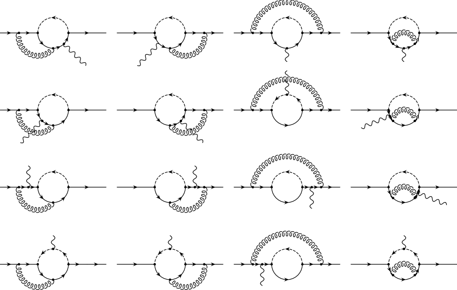
Figure 1: One-particle irreducible two-loop diagrams for $b\to sl^{+}l^{-}$ needed to extract the charged Higgs boson contribution to $C_{9}^{(2)}(\mu_{W})$ and $C_{10}^{(2)}(\mu_{W})$. The external quark lines (solid) denote the incoming $b$-quark and the outgoing $s$-quark, while the wavy line denotes a virtual photon or a $Z^{0}$-boson, which decays into a $l^{+}l^{-}$-pair. The internal dashed-, solid- and curly lines denote the charged Higgs boson $H^{\pm}$, the $t$-quark and the gluon, respectively.

After using heavy mass expansion techniques [12], partial fraction decomposition and the usual reduction of tensor integrals to scalar ones, we obtain integrals of the type

$$C^{(2)}_{n_{1}n_{2}n_{3}} = \frac{(m_{1}^{2})^{n_{1}+n_{2}+n_{3}-4+2\epsilon}}{\pi^{4-2\epsilon}\;\Gamma(1+\epsilon)^{2}}\int\frac{d^{4-2\epsilon}q_{1}\;d^{4-2\epsilon}q_{2}}{(q_{1}^{2}-m_{1}^{2})^{n_{1}}(q_{2}^{2}-m_{2}^{2})^{n_{2}}[(q_{1}-q_{2})^{2}]^{n_{3}}},$$ (8)

which are known explicitly [13, 14].

Note that only the contributions from the internal top-quarks have to be taken into account in these diagrams, because the charm contributions, which come with a relative suppression factor of $m_{b}m_{c}/m_{t}^{2}$ or $m_{c}^{2}/m_{t}^{2}$, only induce dimension 8 operators which are neglected in our treatment.

We write the one- and two-loop charged Higgs induced contributions to $C_{9}(\mu_{W})$ and $C_{10}(\mu_{W})$ in the form

$$C_{9,\rm{H}}^{(n)}(\mu_{\scriptscriptstyle W}) = Y^{2}\,\left(\Gamma^{(n)}+\;\frac{1-4s_{W}^{2}}{s_{W}^{2}}\,\,Z^{(n)}\right)\,,$$

$$C_{10,\rm{H}}^{(n)}(\mu_{\scriptscriptstyle W}) = -Y^{2}\,\left(\;\frac{1}{s_{W}^{2}}\,Z^{(n)}\right)\,,$$ (9)

where $s_{W}=\sin\theta_{W}$. The terms proportional to $Z^{(n)}$ ($\Gamma^{(n)}$) account for the $n$-loop $Z^{0}$- (photon-) penguin diagrams.

The one-loop contributions $\Gamma^{(1)}$ and $Z^{(1)}$ read [9]

$$\Gamma^{(1)} = \frac{-\left(38-79\,y+47\,y^{2}\right)y}{108\,{\left(y-1\right)}^{3}}+\frac{\left(4-6\,y+3\,y^{3}\right)y}{18\,{\left(y-1\right)}^{4}}\ln y,$$

$$Z^{(1)} = \frac{xy}{8\,\left(y-1\right)}-\frac{xy}{8\,{\left(y-1\right)}^{2}}\ln y,$$ (10)

with

$$x=\frac{m_{t}^{2}}{M_{W}^{2}}\quad;\quad y=\frac{m_{t}^{2}}{M_{H}^{2}}\,.$$ (11)

Note that $\Gamma^{(1)}$ and $Z^{(1)}$ depend via $x$ and $y$ on the renormalization scheme for the $t$-quark mass. To illustrate this dependence, we give our results in the commonly used $\overline{\rm{MS}}$- and pole-mass scheme. The relation between these mass definitions is given by

$${\overline{m}}_{t}(\mu_{W})=m_{t}^{\rm{pole}}\left(1+\frac{2\alpha_{\scriptscriptstyle S}(\mu_{W})}{\pi}\,\ln\frac{m_{t}^{\rm{pole}}}{\mu_{W}}-\frac{4}{3}\frac{\alpha_{\scriptscriptstyle S}(\mu_{W})}{\pi}\right)+{\cal O}(\alpha_{s}^{2})\,,$$ (12)

where $\overline{m}_{t}(\mu_{W})$ and $m_{t}^{\rm{pole}}$ are the top-quark mass in the $\overline{\rm{MS}}$-scheme and pole-mass scheme, respectively.

The new two-loop terms $\Gamma^{(2)}$ and $Z^{(2)}$, which explicitly depend on the top-mass renormalization scheme, can be written as

$$\Gamma^{(2)} = W_{\Gamma}+N_{\Gamma}\ln\frac{{\mu_{W}}^{2}}{M_{H}^{2}}+\left(\ln\frac{m_{t}^{2}}{\mu_{W}^{2}}-\frac{4}{3}\right)T_{\Gamma}\,,$$

$$Z^{(2)} = W_{Z}+N_{Z}\ln\frac{{\mu_{W}}^{2}}{M_{H}^{2}}+\left(\ln\frac{m_{t}^{2}}{\mu_{W}^{2}}-\frac{4}{3}\right)T_{Z}\,.$$ (13)

The expressions for $W_{\Gamma}$, $N_{\Gamma}$, $W_{Z}$ and $N_{Z}$ are the same in both schemes (up to the different $m_{t}$ in the definition of $x$ and $y$):

$$W_{\Gamma} = \frac{\left(764+3927\,y-9138\,y^{2}+6175\,y^{3}\right)y}{729\,{\left(y-1\right)}^{4}}$$

$$-\frac{4\left(32+18\,y-132\,y^{2}+95\,y^{3}\right)y}{81\,{\left(y-1\right)}^{4}}{\rm Li}_{2}\left(\frac{y-1}{y}\right)$$

$$-\frac{4\,\left(-110+797\,y-1233\,y^{2}+602\,y^{3}+88\,y^{4}\right)y}{243\,{\left(y-1\right)}^{5}}\,\ln y$$

$$+\frac{8\,\left(16+5\,y-57\,y^{2}+54\,y^{3}\right)y}{81\,{\left(y-1\right)}^{5}}\,\ln^{2}y,$$

$$N_{\Gamma} = \frac{4\,\left(263-486\,y+243\,y^{2}+88\,y^{3}\right)y}{243\,{\left(y-1\right)}^{4}}-\frac{8\,\left(16+5\,y-57\,y^{2}+54\,y^{3}\right)y}{81\,{\left(y-1\right)}^{5}}\ln y,$$

$$W_{Z} = \frac{4\left(-3+y\right)xy}{3{\left(y-1\right)}^{2}}+\frac{\left(2-y\right)xy}{{\left(y-1\right)}^{2}}{\rm Li}_{2}\left(\frac{y-1}{y}\right)$$

$$+\frac{\left(2+9\,y-3\,y^{2}\right)xy}{3{\left(y-1\right)}^{3}}\ln y-\frac{2xy}{{\left(y-1\right)}^{3}}\ln^{2}y,$$

$$N_{Z} = \frac{(-3+y)xy}{(y-1)^{2}}+\frac{2xy}{(y-1)^{3}}\ln y\,,$$ (14)

where the function ${\rm Li}_{2}(z)$ is defined as

$${\rm Li}_{2}(z) = -\int_{0}^{z}\frac{dt}{t}\ln(1-t)\,.$$ (15)

The expressions for $T_{\Gamma}$ and $T_{Z}$ depend on the renormalization scheme used for $m_{t}$:

$$\overline{\rm{MS}}-\rm{scheme}:T_{\Gamma} = 0,$$

$$T_{Z} = 0,$$

$$\rm{pole-scheme}:T_{\Gamma} = \frac{4\,\left(31-59\,y+31\,y^{2}+9\,y^{3}\right)y}{27\,{\left(y-1\right)}^{4}}-\frac{16\,\left(1-3\,y^{2}+3\,y^{3}\right)y}{9\,{\left(y-1\right)}^{5}}\ln y,\,$$

$$T_{Z} = \frac{(3-4\,y+y^{2})xy}{{\left(y-1\right)}^{3}}+\frac{2xy}{{\left(y-1\right)}^{3}}\ln y.$$ (16)

3.3 Impact of the two-loop contributions on $C_{10,\rm{H}}$

In this section we briefly illustrate the impact of the two-loop corrections presented in this letter on $C_{10,\rm{H}}(\mu)$. We introduce a rescaled Wilson coefficient (see eq. (6))

$$\hat{C}_{10,\rm{H}}(\mu_{W})\doteq\frac{1}{Y^{2}}\,\frac{4\pi}{\alpha_{s}(\mu_{W})}C_{10,\rm{H}}(\mu_{W}),$$ (17)

In fig. 2 we plot the quantities

$$\frac{1}{Y^{2}}C_{10,\rm{H}}^{(1)}(\mu_{W})\quad\mbox{and}\quad\frac{1}{Y^{2}}\left(C_{10,\rm{H}}^{(1)}(\mu_{W})+\frac{\alpha_{s}(\mu_{W})}{4\pi}C_{10,\rm{H}}^{(2)}(\mu_{W})\right),$$ (18)

i.e. two approximations of $\hat{C}_{10,\rm{H}}$ as a function of the charged Higgs boson mass $M_{H}$ for the $\overline{\rm{MS}}$- and for the pole mass scheme of the $t$-quark mass. As input parameters we use $\alpha_{s}(M_{Z})=0.119$, $m_{t}^{\rm{pole}}=178.0~{}{\rm GeV}$, $M_{W}=80.4~{}{\rm GeV}$ and $s^{2}_{W}=0.231$ [15, 16]. The upper frame shows these quantities at the relatively low matching scale $\mu_{W}=M_{W}$. As in this case $m_{t}^{\rm{pole}}$ and $\overline{m}_{t}(\mu_{W})$ are numerically almost identical, the one-loop approximations (dotted and dashed lines) are close to each other. The inclusion of the two-loop corrections, however, considerably lowers the (absolute) size of the coefficient for all values of $M_{H}$ considered. In the lower frame a higher matching scale of $\mu_{W}=300$ GeV is chosen. As in this case $m_{t}^{\rm{pole}}$ and $\overline{m}_{t}(\mu_{W})$ differ considerably, the renormalization scheme dependence of the one-loop results is rather large. When taking into account the two-loop corrections (solid and dash-dotted lines), the scheme dependence is drastically reduced.

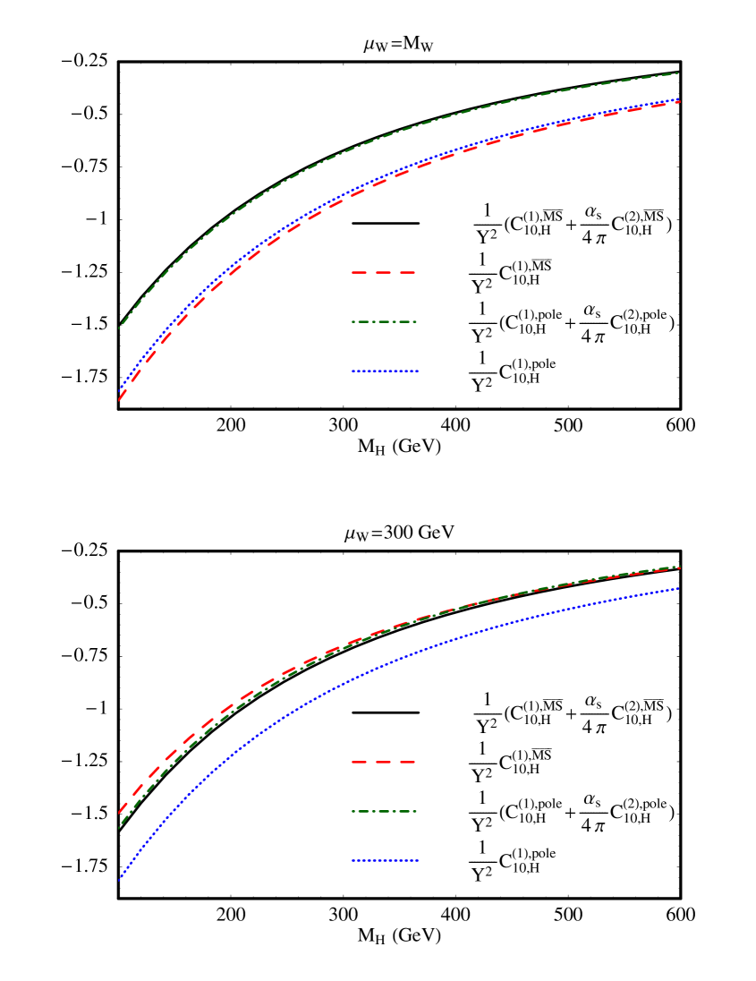
Figure 2: Dependence of the rescaled Wilson coefficient $\hat{C}_{10,\rm{H}}(\mu_{W})$ (see eq. (17)) on the charged Higgs boson mass $M_{H}$ at the matching scale $\mu_{W}=M_{W}$ (upper frame) and $\mu_{W}=300$ GeV (lower frame). The dashed (dotted) line is the one-loop contribution expressed in $\overline{\rm{MS}}$ -scheme (pole-mass scheme) of the $t$-quark mass, while the solid (dash-dotted) line includes the two-loop corrections in the respective scheme.

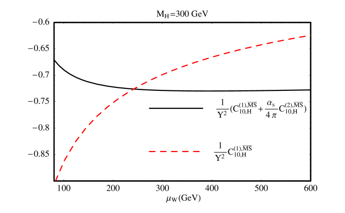
Figure 3: Dependence of the rescaled Wilson coefficient $\hat{C}_{10,\rm{H}}(\mu_{b})$ on the matching scale $\mu_{W}$ (see eq. (17)) for $M_{H}=300$ GeV. The dashed line shows the one-loop contribution expressed in $\overline{\rm{MS}}$ -scheme for the $t$-quark mass, while the solid line includes the two-loop corrections in the same scheme.

Looking at the renormalization group equation (RGE) [17] for $\hat{C}_{10,\rm{H}}$, one finds that $\hat{C}_{10,\rm{H}}$ does not run, i.e.

$$\hat{C}_{10,\rm{H}}(\mu_{b})=\hat{C}_{10,\rm{H}}(\mu_{W})\,,$$ (19)

where the low scale $\mu_{b}$ is of the order of $m_{b}$. In fig. 3 we show the dependence of $\hat{C}_{10,\rm{H}}(\mu_{b})$ on the matching scale $\mu_{W}$ for $M_{H}=300$ GeV. It can be clearly seen that the inclusion of the two-loop contributions drastically lowers the dependence on $\mu_{W}$. For $\mu_{W}>250$ GeV, $\hat{C}_{10,\rm{H}}(\mu_{b})$ at two-loop precision is nearly $\mu_{W}$-independent. For $\mu_{W}$ between $M_{W}$ and 250 GeV the two-loop Wilson coefficient varies about $\pm 4\%$, whereas the corresponding one-loop coefficient varies about $\pm 11\%$.

To summarize: In this letter we have presented QCD corrections to the charged Higgs induced contributions to the Wilson coefficients $C_{9}(\mu_{W})$ and $C_{10}(\mu_{W})$ in type-I and type-II 2HDMs. These two-loop results are important ingredients for complete NNLL calculations of various observables related to the decay $B\to X_{s}l^{+}l^{-}$ in these models.

Just before submitting the present paper, we became aware of the PhD thesis of Ch. Bobeth (http://tumb1.biblio.tu-muenchen.de/publ/diss/ph/2003/bobeth.pdf), where the two-loop results for the charged Higgs boson contribution to $C_{9}$ and $C_{10}$ are contained. We have checked that our results agree.

We would like to thank K. Bieri and D. Wyler for helpful discussions. S.S would like to thank M. Misiak and J. Urban for fruitful discussions and advice regarding the technical details of the two-loop calculations. This work is partially supported by: the Swiss National Foundation; RTN, BBW-Contract No. 01.0357 and EC-Contract HPRN-CT-2002-00311 (EURIDICE).

References

- [1] P. Gambino and M. Misiak, Nucl. Phys. B 611 (2001) 338 [arXiv:hep-ph/0104034].
- [2] M. Ciuchini, G. Degrassi, P. Gambino and G. F. Giudice, Nucl. Phys. B 527 (1998) 21 [arXiv:hep-ph/9710335].
-
[3]
F. M. Borzumati and C. Greub,
Phys. Rev. D 58 (1998) 074004 [arXiv:hep-ph/9802391];
F. M. Borzumati and C. Greub, Phys. Rev. D 59 (1999) 057501 [arXiv:hep-ph/9809438]. - [4] P. Ciafaloni, A. Romanino and A. Strumia, Nucl. Phys. B 524 (1998) 361 [arXiv:hep-ph/9710312].
- [5] C. Bobeth, M. Misiak and J. Urban, Nucl. Phys. B 567 (2000) 153 [arXiv:hep-ph/9904413].
- [6] S. Schilling, in preparation.
- [7] S. L. Glashow and S. Weinberg, Phys. Rev. D 15 (1977) 1958.
- [8] S. Bertolini, F. Borzumati, A. Masiero and G. Ridolfi, Nucl. Phys. B 353 (1991) 591.
- [9] P. L. Cho, M. Misiak and D. Wyler, Phys. Rev. D 54 (1996) 3329 [arXiv:hep-ph/9601360].
- [10] C. Bobeth, M. Misiak and J. Urban, Nucl. Phys. B 574 (2000) 291 [arXiv:hep-ph/9910220].
- [11] C. Greub and T. Hurth, Phys. Rev. D 56 (1997) 2934 [arXiv:hep-ph/9703349].
- [12] V. A. Smirnov, Mod. Phys. Lett. A 10 (1995) 1485 [arXiv:hep-th/9412063].
- [13] A. I. Davydychev and J. B. Tausk, Nucl. Phys. B 397 (1993) 123.
- [14] A. Ghinculov and J. J. van der Bij, Nucl. Phys. B 436 (1995) 30 [arXiv:hep-ph/9405418].
- [15] K. Hagiwara et al. [Particle Data Group Collaboration], Phys. Rev. D 66 (2002) 010001.
- [16] V. M. Abazov et al. [D0 Collaboration], Nature 429 (2004) 638 [arXiv:hep-ex/0406031].
- [17] P. Gambino, M. Gorbahn and U. Haisch, Nucl. Phys. B 673 (2003) 238 [arXiv:hep-ph/0306079].