The Three-Loop Splitting Functions in QCD

Abstract

We have computed the next-to-next-to-leading-order (NNLO) contributions to the evolution of unpolarized parton distributions in perturbative QCD [1,2]. In this talk, we briefly recall why this huge computation was necessary and outline how it was performed. We then illustrate the structure of the results and discuss their end-point limits which include the three-loop cusp anomalous dimensions of the Wilson lines. Finally the numerical impact of the new contributions is illustrated.

1 Introduction

For the next decade, the highest-energy experiments in particle physics will be done at the (anti-)proton–proton colliders Tevatron and LHC. At such machines, if we disregard power corrections and observables involving final-state fragmentation functions, the cross sections for hard processes $h$ can be schematically written as

$$\sigma_{h}^{\,pp}\>=\>\sum_{f,f^{\prime}}f_{p}\ast f^{\prime}_{p}\ast\hat{\sigma}_{h}^{\,\rm f\>\!f^{\prime}}\>\>.$$ (1.1)

Here $f_{p}$ stands for the universal momentum distributions of the partons $f$ in the proton, $f=q_{i},\bar{q}_{i},g$ with $i=1,\ldots,{n_{\!f}}$, where ${n_{\!f}}$ is the number of effectively massless

quark flavours. $\hat{\sigma}_{h}^{\,\rm f\>\!f^{\prime}}$ represent the hard (partonic) cross sections for the process under consideration. Hence quantitative studies of the standard model, and of expected and unexpected new particles, require a precise understanding of the partonic luminosities and of the QCD corrections to the corresponding cross sections.

For many important processes, like Higgs-boson production, the second-order (NNLO) QCD corrections need to be taken into account, i.e., the third term in

$$\hat{\sigma}_{h}\>=\>a_{\rm s}^{n_{h}}\,\left[\,\hat{\sigma}_{h}^{(0)}+a_{\rm s}\,\hat{\sigma}_{h}^{(1)}+\,a_{\rm s}^{2}\,\hat{\sigma}_{h}^{(2)}+\ldots\,\right]\>\>.$$ (1.2)

The consistent inclusion of $\hat{\sigma}_{h}^{(2)}$ in Eq. (1.1) requires parton distributions evolved with the corresponding (process-independent) NNLO splitting functions

$$P_{\>\!\rm f\>\!f^{\prime}}^{\,\rm NNLO}\>=\>a_{\rm s}P_{\>\!\rm f\>\!f^{\prime}}^{(0)}+a_{\rm s}^{2}P_{\>\!\rm f\>\!f^{\prime}}^{(1)}+a_{\rm s}^{3}P_{\>\!\rm f\>\!f^{\prime}}^{(2)}\>\>.$$ (1.3)

The one- and two-loop splitting functions have been known for a long time [3]–[11]. For the three-loop splitting functions $P^{(2)}$, on the other hand, only partial results had been obtained until recently [12]–[22]. However earlier this year we have, finally, computed the complete expressions of these functions [1, 2].

2 Outline of the calculation

We have derived the NNLO splitting functions by computing the partonic structure functions in inclusive deep-inelastic scattering (DIS), $\gamma^{\ast}(q)+f(p)\rightarrow X$ with $Q^{2}\equiv-q^{2}>0$ and $p^{2}=0$, up to the third order in the strong coupling $a_{\rm s}=\alpha_{\rm s}/(4\pi)$. This computation has been performed for all even or odd values of the Mellin variable $N$ via the three-loop forward Compton amplitudes, $\gamma^{\ast}(q)+f(p)\rightarrow\gamma^{\ast}(q)+f(p)$.

This approach has two major advantages: Firstly it enables us to obtain, at almost the same time, also the three-loop coefficient functions in DIS [23]. Secondly it allows us to check our programs, at almost any stage, by falling back to the Mincer program [24, 25] employed in the fixed-$N$ calculations of refs. [12]–[14].

2.1 Mass-factorization in DIS

Before we address the main computational task, we briefly sketch how the splitting functions are extracted from the calculation. We start by writing the physical structure functions $F_{a}$ in terms of the (perturbatively calculable) bare partonic structure functions $\tilde{F}_{a,k}$, the bare coupling $\tilde{a}_{\rm s}$ and the bare parton distributions $\tilde{f}_{k}$,

$$F_{a}(Q^{2})\>=\>\tilde{F}_{a,k}(\tilde{a}_{\rm s},Q^{2},\varepsilon)\ast\tilde{f}_{k}\>\>.$$ (2.1)

Summation over the parton species $k$ is understood, and $\ast$ stands for either the convolution in Bjorken-$x$ space or a simple multiplication of the Mellin moments. As indicated in Eq. (2.1), we use dimensional regularization with $D=4-2\varepsilon$, thus the singularities of $\tilde{F}_{a,k}$ appear as poles $\varepsilon^{-l}$. After the ultraviolet divergences have been removed by coupling-constant renormalization, at the renormalization scale $\mu_{r}$, only initial-state mass singularities remain. They arise when two momenta become collinear, e.g., $p$ and $k$ in Fig. 1, leading to propagator denominators

$$(p-k)^{2}\,=\,-2|\vec{p}\,||\vec{k}|(1-\cos\vartheta)\,\stackrel{{\scriptstyle\vartheta\rightarrow 0}}{{-\!\!\!-\!\!\!\longrightarrow}}\,-|\vec{p}\,||\vec{k}|\vartheta^{2}\>\>.$$

These singularities are removed by mass factorization, at the factorization scale $\mu_{f}$: $\tilde{F}_{a,k}$ is decomposed into finite pieces, the coefficient functions $C_{a,i}$, and the universal transition functions $\Gamma_{ik}$ which contain the ($a$-independent) pole parts of $\tilde{F}_{a,k}$. The latter are combined with the $\tilde{f}_{k}$ to form the finite renormalized parton densities $f_{i}$,

$$F_{a}(Q^{2}) \>=\> \tilde{F}_{a,k}\big{(}a_{\rm s}(\mu_{r}^{2}),\frac{Q^{2}}{\mu_{r}^{2}},\varepsilon\big{)}\ast\tilde{f}_{k}$$ (2.2)

$$\>=\> {C_{a,i}\big{(}a_{\rm s}(\mu_{r}^{2}),\frac{Q^{2}}{\mu_{f}^{\,}2},\frac{\mu_{f}^{\,2}}{\mu_{r}^{2}}\big{)}}\ast\overbrace{\Gamma_{ik}\big{(}a_{\rm s}(\mu_{r}^{2}),\frac{\mu_{f}^{\,2}}{\mu_{r}^{2}},\varepsilon\big{)}\ast\tilde{f}_{k}}^{{\textstyle f_{i}(\mu^{2}_{\,f_{\,{}_{\!}}},\mu_{r}^{2})}}\>\>.$$

The decomposition (2.2) is not unique. We employ the usual $\overline{\mbox{MS}}$ scheme where, besides the $1/\varepsilon$ poles, only the artefacts $S_{\varepsilon}=\exp(\varepsilon[\,\ln(4\pi)-\gamma_{e}])$ of dimensional regularization are removed from the coefficient functions. Differentiation of Eq. (2.2) finally leads to the evolution equations for the renormalized parton distributions,

$$\frac{\partial}{\partial\ln\mu_{f}^{\,2}}\,f_{i}\>=\>\frac{\partial\,\Gamma_{ik}}{\partial\ln\mu_{f}^{\,2}}\,\ast\tilde{f}_{k}\>=\>\frac{\partial\,\Gamma_{ik}}{\partial\ln\mu_{f}^{\,2}}\,\ast\Gamma^{-1}_{kj}\ast f_{j}\>\equiv\>P_{ij}\ast f_{j}\>\>.$$ (2.3)

The splitting functions (1.3) can thus be obtained from the $1/\varepsilon$ poles in Eq. (2.2).

Figure 1: Sample diagrams contributing to the inclusive process $\gamma^{\ast}g\rightarrow X$ up to third order in $a_{\rm s}$.

2.2 The flavour decomposition

It is convenient to decompose the system (2.3) of $2n_{f}\!+\!1$ coupled equation as far as possible from charge conjugation and flavour symmetry constraints alone. The general structure of the (anti-)quark (anti-)quark splitting functions reads

$$P_{{\rm q}_{i}{\rm q}_{k}}\>=\>P_{\bar{{\rm q}}_{i}\bar{{\rm q}}_{k}} \!=\! \delta_{ik}P_{{\rm q}{\rm q}}^{\,\rm v}+P_{{\rm q}{\rm q}}^{\,\rm s}$$

$$P_{{\rm q}_{i}\bar{{\rm q}}_{k}}\>=\>P_{\bar{{\rm q}}_{i}{\rm q}_{k}} \!=\! \delta_{ik}P_{{\rm q}\bar{{\rm q}}}^{\,\rm v}+P_{{\rm q}\bar{{\rm q}}}^{\,\rm s}\>\>.$$ (2.4)

This structure leads to three independently evolving types of flavour non-singlet combinations. The flavour asymmetries $q_{\rm ns}^{\,\pm}$ and the total valence distribution $q_{\rm ns}^{\rm v}$,

$$q_{{\rm ns},ik}^{\,\pm}\>=\>q_{i}\pm\bar{q}_{i}-(q_{k}\pm\bar{q}_{k})\>\>,\quad{\textstyle q_{\rm ns}^{\rm v}\>=\>\sum_{r=1}^{{n_{\!f}}}\,(q_{r}-\bar{q}_{r})}\>\>,$$ (2.5)

respectively evolve with

$$P_{\rm ns}^{\,\pm} \>=\> P_{{\rm q}{\rm q}}^{\,\rm v}\pm P_{{\rm q}\bar{{\rm q}}}^{\,\rm v}\>\>,$$

$$P_{\rm ns}^{\,\rm v} \>=\> P_{\rm qq}^{\,\rm v}-P_{{\rm q}\bar{{\rm q}}}^{\,\rm v}+{n_{\!f}}(P_{\rm qq}^{\,\rm s}-P_{{\rm q}\bar{{\rm q}}}^{\,\rm s})\>\equiv\>P_{\rm ns}^{\,-}+P_{\rm ns}^{\,\rm s}\>\>.$$ (2.6)

The singlet quark distribution, $q_{\>\!\rm s}\>=\>\sum_{r=1}^{{n_{\!f}}}\,(q_{r}+\bar{q}_{r})$ is coupled to gluon density $g$,

$$\frac{d}{d\ln\mu_{f}^{\,2}}\left(\begin{array}[]{c}\!q_{\>\!\rm s}\!\\ g\end{array}\right)\>=\>\left(\begin{array}[]{cc}P_{\rm qq}&P_{\rm qg}\\ P_{\rm gq}&P_{\rm gg}\end{array}\right)\ast\left(\begin{array}[]{c}\!q_{\>\!\rm s}\!\\ g\end{array}\right)\>\>,$$ (2.7)

where the quark-quark splitting function $P_{\rm qq}$ can be expressed as

$$P_{\rm qq}\>=\>P_{\rm ns}^{\,+}+{n_{\!f}}(P_{\rm qq}^{\>\rm s}+P_{\rm{\bar{q}q}}^{\>\rm s})\>\equiv\>P_{\rm ns}^{\,+}+P_{\rm ps}\>\>.$$ (2.8)

The off-diagonal entries in Eq. (2.7) are given by

$$P_{\rm qg}\>=\>{n_{\!f}}\,P_{{\rm q}_{i}\rm g}\>\>,\quad P_{\rm gq}\>=\>P_{{\rm gq}_{i}}$$ (2.9)

in terms of the flavour-independent splitting functions $P_{{\rm q}_{i}\rm g}=P_{\bar{\rm q}_{i}\rm g}$ and $P_{{\rm gq}_{i}}=P_{{\rm g}\bar{\rm q}_{i}}$.

In the expansion in powers of $a_{\rm s}$, the flavour-diagonal (‘valence’) quantity $P_{\rm qq}^{\,\rm v}$ in Eq. (2.2) starts at first order. $P_{{\rm q}\bar{{\rm q}}}^{\,\rm v}$ and the flavour-independent (‘sea’) contributions $P_{{\rm qq}}^{\,\rm s}$ and $P_{{\rm q}\bar{{\rm q}}}^{\,\rm s}$ – and hence the ‘pure-singlet’ term $P_{\rm ps}$ – are of order $\alpha_{\rm s}^{2}$. A non-vanishing $P_{\rm ns}^{\,\rm s}=P_{{\rm qq}}^{\,\rm s}-P_{{\rm q}\bar{{\rm q}}}^{\,\rm s}$ in Eq. (2.2) occurs for the first time at the third order and introduces a new colour structure, $d_{abc}d_{abc}$. See Fig. 1b of ref. [26] for a typical diagram contributing to $P_{\rm ns}^{\,\rm s}$.

2.3 Set-up of the calculation

Diagrams like those in Fig. 1 have been calculated directly, by working out the phase-space integrations, for the derivation of the complete second-order coefficient functions [27]–[30]. An extension of this procedure to the third order, however, does not seem feasible. Instead, we employ the optical theorem

to transform the problem into forward Compton amplitudes. We then make use of a theorem [31] that the coefficient of $(2p\cdot q)^{N}$ provides the $N$-th Mellin moment,

$$\tilde{F}(N)\>=\>\int_{0}^{1}\!dx\>x^{N-1}\tilde{F}(x)\>\>,$$

of the partonic structure functions (2.1) which we need to calculate.

In order to obtain the complete set of the third-order contributions to the splitting functions (2.2) and (2.7) we have to include, besides the photon shown above, also the $W$-boson [26] – for accessing $P_{\rm ns}^{\,-}$ and $P_{\rm ns}^{\,\rm s}$ – and a fictitious classical scalar $\phi$ coupling directly only to the gluon field via $\phi\,G_{\mu\nu}^{\,a}G_{a}^{\,\mu\nu}$ [32, 33] – for accessing $P_{\rm gq\,}$ and $P_{\rm gg}$. Especially the latter leads to a substantial increase of the number of diagrams (generated with Qgraf [34]) as shown in Table 1. Among the partons $f$ we also include the standard ghost $h$. This allows us to take the sum over external gluon spins by contracting with $-g_{\mu\nu}$ instead of the full physical expression.

tree 1-loop 2-loop 3-loop

q$$\gamma$$ 1 3 025 0359

g 2 017 0345

h 002 0056

q 1 3 032 0589

q 1 023 0696

g 1 8 218 6378

h 1 033 1184

sum 3 18 350 9607

Table 1: The number of diagrams employed in our calculation of the three-loop splitting functions.

Obviously a highly efficient symbolic treatment is needed to cope with the task at hand. Unsurprisingly, we use FORM for all manipulations. Note that the capabilities of this program had to be extended substantially for this computation [35, 36].

2.4 Treatment of the integrals

Finally we illustrate the computation of the integrals required to evaluate the forward Compton amplitudes. One of the 9607 three-loop diagrams in Table 1 is shown here together with a useful pictorial representation of its momentum flow:

For the latter we temporarily disregard the external parton lines and draw the remaining self-energy type diagram, the topology of which is denoted following the notation of ref. [25]. Our example is a ladder (LA) diagram. The (partly additional) denominators carrying the parton momentum $p$ are then indicated by the fat (in the coloured version: red) lines. Here $p$ runs, after turning the diagram upside-down, through the lines 1, 2 and 3, thus the example is assigned the subtopology LA₁₃.

According to our discussion in the previous subsection, we need analytic expressions for the (dimensionless) coefficients $I(N)$ of $(2p\cdot q)^{N}/Q^{2\alpha}$. One might try to obtain $I(N)$ by brute force, Taylor-expanding the denominators with $p$ and working out the sums. It turns out that such a strategy, in general, does not work. Instead, we employ identities based on integration by parts, scaling arguments and form-factor decompositions (see Sect. 2 of ref. [1]) to successively simplify the integrals.

The LA₁₃ integrals, e.g., can be simplified by applying $p^{\mu}\partial/\partial q^{\mu}$ both inside and outside the integral. For the scalar integral with unit denominators this yields

$$-\frac{N\!+\!3\!+\!3\epsilon}{N\!+\!2}\,\frac{2p\!\cdot\!q}{q^{2}}\raisebox{-34.0pt}{ \begin{picture}(50.0,20.0)(0.0,-3.0) \put(0.0,0.0){} \put(0.0,0.0){} \put(0.0,0.0){} \put(0.0,0.0){} \put(0.0,0.0){} \put(0.0,0.0){} \put(0.0,0.0){} \put(0.0,0.0){} { \put(0.0,0.0){} \put(0.0,0.0){} \put(0.0,0.0){} } { } \put(0.0,0.0){\makebox(0.0,0.0)[]{}} { } \put(0.0,0.0){\makebox(0.0,0.0)[]{}} { } \put(0.0,0.0){\makebox(0.0,0.0)[]{}} { } \put(0.0,0.0){\makebox(0.0,0.0)[]{}} { } \put(0.0,0.0){\makebox(0.0,0.0)[]{}} { } { } \put(0.0,0.0){\makebox(0.0,0.0)[]{}} { } \put(0.0,0.0){\makebox(0.0,0.0)[]{}} { } { } \put(0.0,0.0){\makebox(0.0,0.0)[]{}} { } \put(0.0,0.0){\makebox(0.0,0.0)[]{}} { } \put(0.0,0.0){\makebox(0.0,0.0)[]{}} \end{picture} }\hskip 51.21504pt\!\!+\frac{2}{N\!+\!2}\raisebox{-34.0pt}{ \begin{picture}(50.0,20.0)(0.0,-3.0) \put(0.0,0.0){} \put(0.0,0.0){} \put(0.0,0.0){} \put(0.0,0.0){} \put(0.0,0.0){} \put(0.0,0.0){} \put(0.0,0.0){} \put(0.0,0.0){} { \put(0.0,0.0){} \put(0.0,0.0){} } { } \put(0.0,0.0){\makebox(0.0,0.0)[]{}} { } \put(0.0,0.0){\makebox(0.0,0.0)[]{}} { } \put(0.0,0.0){\makebox(0.0,0.0)[]{}} { } \put(0.0,0.0){\makebox(0.0,0.0)[]{}} { } \put(0.0,0.0){\makebox(0.0,0.0)[]{}} { } { } \put(0.0,0.0){\makebox(0.0,0.0)[]{}} { } { } \put(0.0,0.0){\makebox(0.0,0.0)[]{}} { } \put(0.0,0.0){\makebox(0.0,0.0)[]{}} { } \put(0.0,0.0){\makebox(0.0,0.0)[]{}} \end{picture} }$$

Here the LA₁₃ integral occurs twice, once with a prefactor $2p\cdot q$. Hence Eq. (2.10) represents a difference equation (here of order $n=1$) which expresses its coefficient $I(N)$ in terms of that of a LA₁₂ integral with an enhanced denominator in the 3-line,

$$a_{0}(N)I(N)-\dots-a_{n}(N)I(N\!-\!n)-G(N)=0\>\>.$$ (2.11)

First-order recursion relations like Eq. (2.10) can be reduced to a sum. Higher-order recursions (we have used equations up to $n=4$) can be solved by inserting a suitable ansatz into Eq. (2.11). Both procedures make use of the fact that all integrals required for the computation of the splitting functions can be expressed in terms of harmonic sums [37]. Recall that these sums are recursively defined by

$$S_{\pm m}(M)\>=\>\sum_{i=1}^{M}\>\frac{(\pm 1)^{i}}{i^{\,m}}\>\>,\quad S_{\pm m_{1},m_{2},\ldots,m_{k}}(M)\>=\>\sum_{i=1}^{M}\>\frac{(\pm 1)^{i}}{i^{\,m_{1}}}\>S_{m_{2},\ldots,m_{k}}(i)\>\>.$$ (2.12)

To the accuracy in the dimensional offset $\varepsilon$ required for the calculation of the splitting functions, our example integral reads, using the Form notations den(i+N) for $1/(N\!+\!i)$ and S(R(m1,...,mk),i+N) for $S_{m_{1},\ldots,m_{k}}(N\!+\!i)$,

 +theta(N)*sign(N)*ep^-2*(-8/3*den(1+N)^2-4*den(1+N)^3+8/3*den(1+N)^2*S(R(
    1),1+N)+4/3*den(1+N)*S(R(1),1+N)+2/3*den(1+N)*S(R(2),1+N)-4/3*den(2+N)
    ^2-2*den(2+N)^3+4/3*den(2+N)^2*S(R(1),2+N)+4/3*den(2+N)*S(R(1),2+N)+2/
    3*den(2+N)*S(R(2),2+N)+4/3*S(R(1),N)+2/3*S(R(1,2),N)-2*S(R(2),N)-4/3*
    S(R(2),N)*N+4*S(R(2,1),N)+4/3*S(R(2,1),N)*N-6*S(R(3),N)-2*S(R(3),N)*N)

 +theta(N)*sign(N)*ep^-1*(32*den(1+N)^2+164/3*den(1+N)^3+24*den(1+N)^4-20/
    3*den(1+N)^3*S(R(1),1+N)-88/3*den(1+N)^2*S(R(1),1+N)+8/3*den(1+N)^2*S(
    R(1,1),1+N)-40/3*den(1+N)^2*S(R(2),1+N)-16*den(1+N)*S(R(1),1+N)+8/3*
    den(1+N)*S(R(1,1),1+N)+10/3*den(1+N)*S(R(1,2),1+N)-58/3*den(1+N)*S(R(2
    ),1+N)+10*den(1+N)*S(R(2,1),1+N)-18*den(1+N)*S(R(3),1+N)+16*den(2+N)^2
    +82/3*den(2+N)^3+12*den(2+N)^4-10/3*den(2+N)^3*S(R(1),2+N)-44/3*den(2+
    N)^2*S(R(1),2+N)-6*den(2+N)^2*S(R(2),2+N)-16*den(2+N)*S(R(1),2+N)+8/3*
    den(2+N)*S(R(1,1),2+N)+10/3*den(2+N)*S(R(1,2),2+N)-46/3*den(2+N)*S(R(2
    ),2+N)+6*den(2+N)*S(R(2,1),2+N)-12*den(2+N)*S(R(3),2+N)-20*S(R(1),N)+8/
    3*S(R(1,1),N)+10/3*S(R(1,1,2),N)-16*S(R(1,2),N)-4*S(R(1,2),N)*N+14*S(
    R(1,2,1),N)+4*S(R(1,2,1),N)*N-24*S(R(1,3),N)-6*S(R(1,3),N)*N+56/3*S(R(
    2),N)+20*S(R(2),N)*N-134/3*S(R(2,1),N)-56/3*S(R(2,1),N)*N+16/3*S(R(2,1
    ,1),N)+8/3*S(R(2,1,1),N)*N-62/3*S(R(2,2),N)-22/3*S(R(2,2),N)*N+76*S(R(
    3),N)+100/3*S(R(3),N)*N-10*S(R(3,1),N)-10/3*S(R(3,1),N)*N+36*S(R(4),N)
    +12*S(R(4),N)*N)  .

Despite being uncharacteristically simple in both derivation and size, Eq. (2.10) illustrates the strict hierarchy of subtopologies in our procedure. Our LA₁₃ example can only be evaluated once the LA₁₂ integral in Eq. (2.10) is known. This integral, in turn, requires the so-called basic building blocks (with only one $p$-dependent denominator) LA₁₁ and LA₂₂ together with other integrals of simpler topologies where one of the non-$p$ denominators has been removed. Also those integrals need to be evaluated in terms of yet simpler cases, and so on.

Constructing the reduction chains for all subtopologies, and computing all integrals required for evaluating either diagrams or other, higher-level integrals took literally years of both human and computing resources. It would not have been possible to get through without extensive tabulation of intermediate results for which new features were added to Form [36]. At the end, a database had been accumulated of more than 100 000 integrals requiring about 3.5 GBytes of disk space.

3 Sample results in $N$-space and $x$-space

We illustrate our final results by writing down the even-$N$ anomalous dimensions and the corresponding $x$-space splitting functions in Quantum-Gluodynamics, i.e., for QCD with ${n_{\!f}}=0$ quark flavours. The complete QCD results in refs. [1, 2] are considerably longer, by a factor of about 15, but not structurally more complicated.

3.1 Expressions in Mellin-$N$ space

We start in $N$-space where, as discussed above, the actual calculations have been performed. Recall that we expand in terms of $a_{\rm s}=\alpha_{\rm s}/(4\pi)$, and that $\gamma^{\,(n)}(N)\!=!-P^{\,(n)}(N)$ is the coefficient of $a_{\rm s}^{\,n+1}$. Here we hide $N$-dependent denominators by using differences of harmonic sums at suitably shifted arguments for which we employ the abbreviations

$${{\bf N_{\pm i}}}\,S_{\vec{m}}\equiv S_{\vec{m}}(N\pm i)\>\>,\quad{{\bf N_{\pm}}}\equiv{{\bf N_{\pm 1}}}\>\>.$$

In this notation the well-known one- and two-loop results [3, 4, 7, 10, 11] are given by

$$\gamma^{\,(0)}_{\,\rm gg}(N)\>=\>{C_{\!A}}\,\*\Big{(}4\,\*({{\bf N_{-2}}}-2\*{{\bf N_{-}}}-2\*{{\bf N_{+}}}+{{\bf N_{+2}}}+3)\,\*{{S}_{1}}-{11\over 3}\Big{)}\>\>,$$ (3.1)

$$\gamma^{\,(1)}_{\,\rm gg}(N)\>=\>4\,\*{C^{\,2}_{\!A}}\*\Big{(}-4\,\*({{\bf N_{-2}}}-2\*{{\bf N_{-}}}-2\*{{\bf N_{+}}}+{{\bf N_{+2}}}+3)\*\Big{[}{{S}_{1,-2}}+{{S}_{1,2}}+{{S}_{2,1}}\Big{]}$$

$$\mbox{}+{8\over 3}\*({{\bf N_{+}}}-{{\bf N_{+2}}})\*{{S}_{2}}-4\*({{\bf N_{-}}}-3\*{{\bf N_{+}}}+{{\bf N_{+2}}}+1)\*\Big{[}3\*{{S}_{2}}-{{S}_{3}}\Big{]}+{109\over 18}\*({{\bf N_{-}}}+{{\bf N_{+}}})\*{{S}_{1}}$$

$$\mbox{}+{61\over 3}\*({{\bf N_{-}}}-{{\bf N_{+}}})\*{{S}_{2}}-{8\over 3}+2\*{{S}_{-3}}-{14\over 3}\*{{S}_{1}}+2\*{{S}_{3}}\Big{)}\>\>.$$ (3.2)

The three-loop gluon-gluon anomalous dimension [2] reads, for $n_{f}=0$,

$$\gamma^{\,(2)}_{\,\rm gg}(N)\>=\>16\,\*{C^{\,3}_{\!A}}\*\Big{(}({{\bf N_{-2}}}-2\*{{\bf N_{-}}}-2\*{{\bf N_{+}}}+{{\bf N_{+2}}}+3)\*\Big{[}{73091\over 648}\*{{S}_{1}}-16\*{{S}_{1,-4}}+{88\over 3}\*{{S}_{1,-3}}$$

$$\mbox{}+16\*{{S}_{1,-3,1}}+{85\over 6}\*{{S}_{1,-2}}+4\*{{S}_{1,-2,-2}}-11\*{{S}_{1,-2,1}}+4\*{{S}_{1,-2,2}}-{413\over 108}\*{{S}_{1,1}}+24\*{{S}_{1,1,-3}}$$

$$\mbox{}+11\*{{S}_{1,1,-2}}-16\*{{S}_{1,1,-2,1}}+8\*{{S}_{1,1,3}}-{67\over 9}\*{{S}_{1,2}}+8\*{{S}_{1,2,-2}}+8\*{{S}_{1,2,2}}+{55\over 3}\*{{S}_{1,3}}+8\*{{S}_{1,3,1}}$$

$$\mbox{}-8\*{{S}_{1,4}}-{395\over 27}\*{{S}_{2}}-14\*{{S}_{2,-3}}-{11\over 3}\*{{S}_{2,-2}}+8\*{{S}_{2,-2,1}}-{67\over 9}\*{{S}_{2,1}}+4\*{{S}_{2,1,-2}}+8\*{{S}_{2,1,2}}$$

$$\mbox{}+{22\over 3}\*{{S}_{2,2}}+8\*{{S}_{2,2,1}}-10\*{{S}_{2,3}}+8\*{{S}_{3,1,1}}-8\*{{S}_{3,2}}\Big{]}+(2-{{\bf N_{-}}}-{{\bf N_{+}}})\*\Big{[}{713\over 324}\*{{S}_{1}}+{26\over 3}\*{{S}_{1,-3}}$$

$$\mbox{}-14\*{{S}_{1,-2,1}}+{61\over 9}\*{{S}_{1,-2}}+{80\over 27}\*{{S}_{1,1}}-14\*{{S}_{1,1,-2}}+{109\over 18}\*{{S}_{1,2}}-4\*{{S}_{1,3}}\Big{]}+({{\bf N_{-}}}-{{\bf N_{+}}})\*\Big{[}{473\over 216}\*{{S}_{2}}$$

$$\mbox{}-12\*{{S}_{2,-3}}+5\*{{S}_{2,-2}}-2\*{{S}_{2,1}}-8\*{{S}_{2,1,-2}}+{23\over 3}\*{{S}_{2,2}}-10\*{{S}_{2,3}}+{665\over 36}\*{{S}_{3}}-20\*{{S}_{3,-2}}+{34\over 3}\*{{S}_{3,1}}$$

$$\mbox{}-16\*{{S}_{3,2}}-21\*{{S}_{4}}-26\*{{S}_{4,1}}\Big{]}+({{\bf N_{-}}}-{{\bf N_{+2}}})\*\Big{[}-{9533\over 108}\*{{S}_{2}}+8\*{{S}_{2,-3}}-{77\over 3}\*{{S}_{2,-2}}-8\*{{S}_{2,-2,1}}$$

$$\mbox{}-8\*{{S}_{2,1,-2}}-{44\over 3}\*{{S}_{2,2}}-{1517\over 18}\*{{S}_{3}}+8\*{{S}_{3,-2}}-{121\over 3}\*{{S}_{3,1}}+4\*{{S}_{3,2}}+44\*{{S}_{4}}+16\*{{S}_{4,1}}-8\*{{S}_{5}}\Big{]}$$

$$\mbox{}+(1-{{\bf N_{+}}})\*\Big{[}{8533\over 108}\*{{S}_{2}}-8\*{{S}_{2,-3}}+{103\over 3}\*{{S}_{2,-2}}+8\*{{S}_{2,-2,1}}+{109\over 9}\*{{S}_{2,1}}+8\*{{S}_{2,1,-2}}+{28\over 3}\*{{S}_{2,2}}$$

$$\mbox{}+{1579\over 18}\*{{S}_{3}}+8\*{{S}_{3,-2}}+{71\over 3}\*{{S}_{3,1}}-4\*{{S}_{3,2}}-{98\over 3}\*{{S}_{4}}-16\*{{S}_{4,1}}+36\*{{S}_{5}}\Big{]}-{79\over 32}+4\*{{S}_{-5}}-8\*{{S}_{-4,1}}$$

$$\mbox{}+{67\over 9}\*{{S}_{-3}}-4\*{{S}_{-3,-2}}-2\*{{S}_{-3,2}}-4\*{{S}_{-2,-3}}-{11\over 3}\*{{S}_{-2,-2}}+4\*{{S}_{-2,-2,1}}+4\*{{S}_{-2,1,-2}}$$

$$\mbox{}-{16619\over 162}\*{{S}_{1}}-{88\over 3}\*{{S}_{1,-3}}-{523\over 18}\*{{S}_{1,-2}}+11\*{{S}_{1,-2,1}}+{413\over 108}\*{{S}_{1,1}}-11\*{{S}_{1,1,-2}}-{67\over 9}\*{{S}_{1,2}}$$

$$\mbox{}-{33\over 2}\*{{S}_{1,3}}+{781\over 54}\*{{S}_{2}}-4\*{{S}_{2,-3}}+{11\over 3}\*{{S}_{2,-2}}+4\*{{S}_{2,-2,1}}-{67\over 9}\*{{S}_{2,1}}+4\*{{S}_{2,1,-2}}-{22\over 3}\*{{S}_{2,2}}$$

$$\mbox{}+{67\over 9}\*{{S}_{3}}-4\*{{S}_{3,-2}}+{11\over 6}\*{{S}_{3,1}}-2\*{{S}_{3,2}}-8\*{{S}_{4,1}}+4\*{{S}_{5}}\Big{)}\>\>.$$ (3.3)

Note that harmonic sums up to weight $2n+1$ occur at order $\alpha_{\rm s}^{\,n+1}$ (NⁿLO).

We stress that Eqs. (3.2) and (3.3) are directly applicable only for even positive values of $N$, while the lowest-order expression (3.1) holds for any positive integer. For general (non-integer) $N$, $\gamma^{\,(n)}(N)$ can be obtained by numerically evaluating

$$\gamma^{\,(n)}(N)\>=\>-\int_{0}^{1}\!dx\>\,x^{\,N-1}\,P^{\,(n)}(x)$$ (3.4)

using the $x$-space results to which we turn now.

3.2 Expressions in Bjorken-$x$ space

There is a theorem [31] ensuring that the splitting functions $P^{(n)}(x)$ can be uniquely reconstructed from their even-$N$ (or odd-$N$) moments obtained in our calculations. In fact, the close relation between the harmonic sums and the harmonic polylogarithms facilitates an algebraic procedure [38, 39] for the inverse Mellin transform.

For a compact representation of the gluon-gluon splitting functions we use

$$p_{\rm{gg}}(x)\>\equiv\>(1-x)^{-1}+x^{\,-1}-2+x-x^{\,2}$$

and an abbreviation for the harmonic polylogarithms [38],

$$H_{\pm(m+1),\,\pm(n+1),\,\ldots}\>\equiv\>H_{\footnotesize{\underbrace{0,\ldots,0}_{\scriptstyle m}},\,\pm 1,\,{\footnotesize\underbrace{0,\ldots,0}_{\scriptstyle n}},\,\pm 1,\,\ldots}(x)\>\>.$$

The one- and two-loop results [5, 9] for ${n_{\!f}}=0$ can then be written as

$$P^{\,(0)}_{\rm gg}(x)\>=\>{C_{\!A}}\*\Big{(}4\*p_{\rm{gg}}(x)+{11\over 3}\*\delta(1-x)\Big{)}\>\>,$$ (3.5)

$$P^{\,(1)}_{\rm gg}(x)\>=\>4\,\*{C^{\,2}_{\!A}}\*\Big{(}2\*p_{\rm{gg}}(x)\*\Big{[}{67\over 18}-{\zeta_{2}}+{\rm{H}}_{0,0}+2\*{\rm{H}}_{1,0}+2\*{\rm{H}}_{2}\Big{]}-2\*p_{\rm{gg}}(-x)\*\Big{[}{\zeta_{2}}+2\*{\rm{H}}_{-1,0}$$

$$-{\rm{H}}_{0,0}\Big{]}-{67\over 9}\*\Big{(}{1\over x}-x^{2}\Big{)}-{44\over 3}\*x^{2}\*{\rm{H}}_{0}+(1+x)\*\Big{[}{11\over 3}\*{\rm{H}}_{0}+8\*{\rm{H}}_{0,0}-{27\over 2}\Big{]}+27-12\*{\rm{H}}_{0}$$

$$+\delta(1-x)\*\Big{[}{8\over 3}+3\*{\zeta_{3}}\Big{]}\Big{)}\>\>.$$ (3.6)

The corresponding three-loop contribution [2] reads

$$P^{\,(2)}_{\rm gg}(x)\>=\>16\,\*{C^{\,3}_{\!A}}\*\Big{(}p_{\rm{gg}}(x)\*\Big{[}{245\over 24}-{67\over 9}\*{\zeta_{2}}+{11\over 3}\*{\zeta_{3}}-{3\over 10}\*{\zeta_{2}}^{2}-4\*{\rm{H}}_{-3,0}+6\*{\rm{H}}_{-2}\*{\zeta_{2}}+4\*{\rm{H}}_{-2,-1,0}$$

$$+{11\over 3}\*{\rm{H}}_{-2,0}-4\*{\rm{H}}_{-2,0,0}-4\*{\rm{H}}_{-2,2}+{1\over 6}\*{\rm{H}}_{0}-7\*{\rm{H}}_{0}\*{\zeta_{3}}+{67\over 9}\*{\rm{H}}_{0,0}-8\*{\rm{H}}_{0,0}\*{\zeta_{2}}+4\*{\rm{H}}_{0,0,0,0}-6\*{\rm{H}}_{1}\*{\zeta_{3}}$$

$$-4\*{\rm{H}}_{1,-2,0}+{134\over 9}\*{\rm{H}}_{1,0}-6\*{\rm{H}}_{1,0}\*{\zeta_{2}}+{11\over 6}\*{\rm{H}}_{1,0,0}+8\*{\rm{H}}_{1,0,0,0}+8\*{\rm{H}}_{1,1,0,0}+8\*{\rm{H}}_{1,2,0}+8\*{\rm{H}}_{1,3}$$

$$+{134\over 9}\*{\rm{H}}_{2}-4\*{\rm{H}}_{2}\*{\zeta_{2}}+10\*{\rm{H}}_{2,0,0}+8\*{\rm{H}}_{2,1,0}+8\*{\rm{H}}_{2,2}+{11\over 6}\*{\rm{H}}_{3}+10\*{\rm{H}}_{3,0}+8\*{\rm{H}}_{3,1}+8\*{\rm{H}}_{4}\Big{]}$$

$$+\,p_{\rm{gg}}(-x)\*\Big{[}-{67\over 9}\*{\zeta_{2}}+{11\over 2}\*{\zeta_{2}}^{2}-4\*{\rm{H}}_{-3,0}+16\*{\rm{H}}_{-2}\*{\zeta_{2}}+8\*{\rm{H}}_{-2,-1,0}-18\*{\rm{H}}_{-2,0,0}-12\*{\rm{H}}_{-2,2}$$

$$+12\*{\rm{H}}_{-1}\*{\zeta_{3}}+8\*{\rm{H}}_{-1,-2,0}-16\*{\rm{H}}_{-1,-1}\*{\zeta_{2}}+24\*{\rm{H}}_{-1,-1,0,0}+16\*{\rm{H}}_{-1,-1,2}-{134\over 9}\*{\rm{H}}_{-1,0}$$

$$+18\*{\rm{H}}_{-1,0}\*{\zeta_{2}}-16\*{\rm{H}}_{-1,0,0,0}-4\*{\rm{H}}_{-1,2,0}-16\*{\rm{H}}_{-1,3}-{11\over 6}\*{\rm{H}}_{0}\*{\zeta_{2}}-5\*{\rm{H}}_{0}\*{\zeta_{3}}+{67\over 9}\*{\rm{H}}_{0,0}-8\*{\rm{H}}_{0,0}\*{\zeta_{2}}$$

$$+4\*{\rm{H}}_{0,0,0,0}+2\*{\rm{H}}_{2}\*{\zeta_{2}}+2\*{\rm{H}}_{3,0}+8\*{\rm{H}}_{4}\Big{]}+\Big{(}{1\over x}-x^{2}\Big{)}\*\Big{[}{16619\over 162}-{55\over 2}\*{\zeta_{3}}-{11\over 2}\*{\rm{H}}_{0}\*{\zeta_{2}}-{413\over 108}\*{\rm{H}}_{1}$$

$$-{11\over 2}\*{\rm{H}}_{1}\*{\zeta_{2}}-{67\over 9}\*{\rm{H}}_{1,0}+{33\over 2}\*{\rm{H}}_{1,0,0}-{67\over 9}\*{\rm{H}}_{2}+{22\over 3}\*{\rm{H}}_{2,0}\Big{]}+11\*\Big{(}{1\over x}+x^{2}\Big{)}\*\Big{[}-{389\over 198}\*{\zeta_{2}}-{2\over 3}\*{\rm{H}}_{-2,0}$$

$$-{1\over 2}\*{\rm{H}}_{-1}\*{\zeta_{2}}+{\rm{H}}_{-1,-1,0}-{523\over 198}\*{\rm{H}}_{-1,0}+{8\over 3}\*{\rm{H}}_{-1,0,0}+{\rm{H}}_{-1,2}+{71\over 54}\*{\rm{H}}_{0}-{1\over 6}\*{\rm{H}}_{3}\Big{]}+x^{2}\*\Big{[}{85\over 6}\*{\zeta_{2}}$$

$$+33\*{\rm{H}}_{-2,0}+{6409\over 108}\*{\rm{H}}_{0}+33\*{\rm{H}}_{0}\*{\zeta_{2}}-{1249\over 18}\*{\rm{H}}_{0,0}-44\*{\rm{H}}_{0,0,0}-{44\over 3}\*{\rm{H}}_{2,0}-{110\over 3}\*{\rm{H}}_{3}\Big{]}$$

$$+(1-x)\*\Big{[}-{11317\over 108}-4\*{\rm{H}}_{-3,0}-4\*{\rm{H}}_{-2}\*{\zeta_{2}}-8\*{\rm{H}}_{-2,-1,0}-{19\over 3}\*{\rm{H}}_{-2,0}-12\*{\rm{H}}_{-2,0,0}-{263\over 12}\*{\rm{H}}_{0,0}$$

$$-{29\over 3}\*{\rm{H}}_{0,0,0}+{31\over 36}\*{\rm{H}}_{1}-{3\over 2}\*{\rm{H}}_{1}\*{\zeta_{2}}+{27\over 2}\*{\rm{H}}_{1,0}-{25\over 2}\*{\rm{H}}_{1,0,0}\Big{]}+(1+x)\*\Big{[}-{329\over 18}\*{\zeta_{2}}+{11\over 2}\*(1+x)\*{\zeta_{3}}$$

$$-{43\over 5}\*{\zeta_{2}}^{2}-{53\over 2}\*{\rm{H}}_{-1}\*{\zeta_{2}}-3\*{\rm{H}}_{-1,-1,0}-{215\over 6}\*{\rm{H}}_{-1,0}+38\*{\rm{H}}_{-1,0,0}+25\*{\rm{H}}_{-1,2}+{4651\over 216}\*{\rm{H}}_{0}-8\*{\rm{H}}_{0}\*{\zeta_{3}}$$

$$+{27\over 2}\*{\rm{H}}_{0}\*{\zeta_{2}}-22\*{\rm{H}}_{0,0}\*{\zeta_{2}}-{158\over 9}\*{\rm{H}}_{2}-4\*{\rm{H}}_{2}\*{\zeta_{2}}+{29\over 3}\*{\rm{H}}_{2,0}+10\*{\rm{H}}_{2,0,0}-{43\over 6}\*{\rm{H}}_{3}+16\*{\rm{H}}_{3,0}+26\*{\rm{H}}_{4}\Big{]}$$

$$+{53\over 6}\*{\zeta_{2}}+24\*{\zeta_{3}}+2\*{\zeta_{2}}^{2}-16\*{\rm{H}}_{-3,0}+27\*{\rm{H}}_{-2,0}+{601\over 12}\*{\rm{H}}_{0}+{41\over 3}\*{\rm{H}}_{0}\*{\zeta_{2}}-16\*{\rm{H}}_{0}\*{\zeta_{3}}-29\*{\rm{H}}_{0,0}$$

$$-4\*{\rm{H}}_{0,0}\*{\zeta_{2}}-{40\over 3}\*{\rm{H}}_{0,0,0}+28\*x\*{\rm{H}}_{0,0,0,0}+27\*{\rm{H}}_{2}-24\*{\rm{H}}_{2,0}-20\*{\rm{H}}_{3}+\delta(1-x)\*\Big{[}{79\over 32}+{1\over 6}\*{\zeta_{2}}$$

$$+{67\over 6}\*{\zeta_{3}}+{11\over 24}\*{\zeta_{2}}^{2}-5\*{\zeta_{5}}-{\zeta_{2}}\*{\zeta_{3}}\Big{]}\Big{)}\>\>,$$ (3.7)

where, as in Eqs. (3.5) and (3.6), all divergences for $x\rightarrow 1$ are to be read as +-distributions. Functions $H_{\vec{m}}(x)$ up to weight (number of indices) $2n$ occur at NⁿLO.

A Fortran program for the harmonic polylogarithms up to weight four is available [40]. Nevertheless it is useful to have also more compact, if approximate representations of the three-loop splitting functions. Making use of the end-point behaviour discussed in the next section, Eq. (3.7) can be parametrized as [2]

$$P^{(2)}_{\rm gg}(x) \cong \mbox{}+2643.521\>{\cal D}_{0}+4425.894\>\delta(1-x)+3589\>L_{1}-20852\>+3968\>x$$ (3.8)

$$\mbox{}-3363\>x^{2}+4848\>x^{3}+L_{0}L_{1}\>(7305+8757\>L_{0})+274.4\>L_{0}$$

$$\mbox{}-7471\>L_{0}^{2}+72\>L_{0}^{3}-144\>L_{0}^{4}+14214\>x^{\,-1}+2675.8\>x^{\,-1}L_{0}$$

where

$${\cal D}_{\,0}\>\equiv\>1/(1-x)_{+}\>,\quad L_{1}\>\equiv\>\ln(1-x)\>,\quad L_{0}\>\equiv\>\ln x\>\>.$$

This parametrization deviates from the exact expression (3.7) by less than 0.1%, which should be perfectly sufficient for numerical applications. Note that the Mellin transform of Eq. (3.8) can be readily continued to complex values of $N$ as required for the moment-space approach to the analysis of hard processes [41]–[43].

4 Results and surprises for $x\rightarrow 1$ and $x\rightarrow 0$

The end-point behaviour of the splitting functions is of particular interest. The leading contributions for $x\!\rightarrow\!1$ are related to the cusp anomalous dimensions and are thus relevant beyond the context of parton distributions. The perturbative stability at very small $x$, where potentially large $\,\ln^{k}x$ corrections occur, represents a much discussed topic directly relevant to analyses of collider processes.

4.1 The large-$x$ behaviour

Up to Nⁿ⁼²LO, at least, the diagonal $\overline{\mbox{MS}}$-scheme splitting functions are given by

$$P^{\,(n)}_{{\rm aa},x\rightarrow 1}(x)\>=\>\frac{A_{n+1}^{\,\rm a}}{(1-x)_{+}}\>+\>B_{n+1}^{\,\rm a}\>\delta(1-x)\>+\>C_{n+1}^{\,\rm a}\>\ln(1-x)\>+\>{\cal O}(1)\>\>.$$ (4.1)

In fact, the simple +-distribution $1/(1-x)_{+}$ constitutes the leading term to all orders — in contrast to, for example, the coefficient functions in DIS which include terms $[(1-x)^{-1}\ln^{k}(1-x)]_{+}$ — and its coefficients $A_{m}^{\,\rm a}$ form the perturbative expansion of the cusp anomalous dimensions of the respective Wilson lines [44]. For the quark case the known coefficients read, in our normalization,

$$A_{1}^{\,\rm q} = 4\,C_{F}$$

$$A_{2}^{\,\rm q} = 8\,C_{F}\left[\left(\frac{67}{18}-\zeta_{2}\right)C_{A}-\frac{5}{9}\,{n_{\!f}}\right]$$

$$A_{3}^{\,\rm q} = 16\,C_{F}C_{A}^{\,2}\,\left[\frac{245}{24}-\frac{67}{9}\>{\zeta_{2}}+\frac{11}{6}\>{\zeta_{3}}+\frac{11}{5}\>{\zeta_{2}}^{\!\!2}\right]+16\,C_{F}^{\,2}{n_{\!f}}\,\left[-\frac{55}{24}+2\>{\zeta_{3}}\right]\quad$$ (4.2)

$$\mbox{}+16\,C_{F}C_{A}{n_{\!f}}\,\left[-\frac{209}{108}+\frac{10}{9}\>{\zeta_{2}}-\frac{7}{3}\>{\zeta_{3}}\right]\,+\,16\,C_{F}{n^{\,2}_{\!f}}\left[-\frac{1}{27}\,\right]\>\>.$$

The coefficients $A_{m}^{\,\rm g}$ are obtained from Eq. (4.1) by multiplication with $C_{A}/C_{F}$. Note that the ${n_{\!f}}$-independent parts of $A_{m}^{\,\rm a}$ consist of only one (the maximally non-abelian) colour factor as also predicted in ref. [44]. The ${n_{\!f}}\!=\!0$ part of $A_{3}^{\,\rm q}$ and the complete $A_{3}^{\,\rm g}$ are new results of refs. [1] and [2], respectively. Two computations of the ${n_{\!f}}$-contribution to $A_{3}^{\,\rm q}$ were performed two years ago [20, 22], and its ${n^{\,2}_{\!f}}$-part was already obtained in ref. [15]. $A_{3}^{\,\rm q}$ in Eq. (4.1) agrees with the previous numerical estimate [45] which has been widely used in soft-gluon resummation analyses.

It is also interesting that at three loops, as in the previous order, only a single logarithm occurs in Eq. (4.1). Furthermore it turns out that there is an unexpected relation between the corresponding coefficients $C_{n+1}^{\,\rm a}$ and the $A_{n}^{\,\rm a}$, viz [1, 2]

$$C_{1}^{\,\rm a}\>=\>0\>,\quad C_{2}^{\,\rm a}\>=\>(A_{1}^{\,\rm a})^{2}\>,\quad C_{3}^{\,\rm a}\>=\>2\>\!A_{1}^{\,\rm a}A_{2}^{\,\rm a}\>\>.$$ (4.3)

The logarithmic structure of Eq. (4.1) and especially the relation (4.3) call for an explanation and, possibly, a higher-order generalization.

The large-$x$ limit of the quark-gluon and gluon-quark splitting functions reads

$$\textstyle{P^{\,(n)}_{ab,x\rightarrow 1}(x)\>=\>\sum_{i=0}^{2n-1}D_{n,i}^{\,\rm ab}\,\ln^{2n-i}(1\!-\!x)\>+\>{\cal O}(1)\>\>.}$$ (4.4)

See ref. [2] for the three-loop coefficients $D_{2,i}^{\,\rm ab}$. Except for $D_{2,3}^{\,\rm gq}$ these coefficients vanish for the choice $C_{A}=C_{F}={n_{\!f}}$ leading to a $\,{\cal N}=1$ supersymmetric theory.

4.2 The small-$x$ behaviour

We start with the flavour non-singlet contributions which, in the present unpolarized case, are practically far less important then the singlet parts. However, the non-singlet small-$x$ expansion includes two additional powers of $\ln x$ per order, i.e., terms up to $\ln^{\,2n}x$ occur at NⁿLO. Thus the three-loop splitting functions

$$P^{(2)i=\pm,\rm s}_{x\rightarrow 0}(x)\>=\>D_{0}^{\,i}\ln^{4}x\>+\>\ldots\>+\>D_{3}^{\,i}\ln x\>+\>{\cal O}(1)$$ (4.5)

form a presently unique theoretical laboratory for studying the relative size of as many as four small-$x$ logarithms as obtained from a complete (all-$x$) calculation.

The numerical QCD values of the coefficients for $\,i=-\,$ in Eq. (4.5) read

$$D_{0}^{-} \>\cong\> 1.4321$$

$$D_{1}^{-} \>\cong\> 35.556-3.1605\>{n_{\!f}}$$

$$D_{2}^{-} \>\cong\> 399.21-39.704\>{n_{\!f}}+0.5926\>n_{\!f}^{\,2}$$

$$D_{3}^{-} \>\cong\> 1465.9-172.69\>{n_{\!f}}+4.3457\>n_{\!f}^{\,2}\>\>.$$ (4.6)

See ref. [1] for the analytic expressions and the similar case $i=+$. In both cases the leading coefficients $D_{0}$ have been correctly predicted [18] on the basis of the resummation in ref. [46]. Note that the expansion (4.5) alternates for $i=\pm$, and that the coefficients $D_{k}$ rise sharply with $k$. For ${n_{\!f}}=4$ and $\,i=-\,$ shown in Fig. 2, the modulus of the $\ln^{4}x$ ($\ln^{3}x$) contribution is twice as large as that of the next term, $\ln^{3}x$ ($\ln^{2}x$), only at extremely small $x$-values, $x\raisebox{-1.9919pt}{$\>\stackrel{{\scriptstyle<}}{{{\scriptstyle\sim}}}\>$}10^{-14}$ ($3\cdot 10^{-10}$).

The numerical situation is rather different for the $d_{abc}d_{abc}$ contribution $i=\rm s$ [1],

$$D_{0}^{\,\rm s} \,\cong\, +1.4815\>{n_{\!f}}\>\>,\quad D_{1}^{\,\rm s}\,\cong\,-2.9630\>{n_{\!f}}$$

$$D_{2}^{\,\rm s} \,\cong\, +6.8918\>{n_{\!f}}\>\>,\quad D_{3}^{\,\rm s}\,\cong\,+178.03\>{n_{\!f}}\>\>.$$ (4.7)

Here the leading small-$x$ terms do indeed provide a reasonable approximation, see Fig. 2. Note that the existence of a leading ($\ln^{4}x$) $d_{abc}d_{abc}$ contribution for $i=\rm s$ is rather surprising. In fact, the presence of a leading small-$x$ logarithm in a term unpredictable from lower-order structures appears to call into question the very concept of the small-$x$ resummation of the double logarithms $\alpha_{\rm s}^{n+1}\ln^{\,2n}x$.

The leading small-$x$ terms of the three-loop singlet splitting functions are

$$P^{(2)}_{{\rm ab},x\rightarrow 0}(x)\>=\>E_{1}^{\,\rm ab}\>\frac{\ln x}{x}\>+\>E_{2}^{\,\rm ab}\>\frac{1}{x}\>+\>{\cal O}(\ln^{\,4}x)\>\>.$$ (4.8)

In general, $x^{-1}\ln^{\,k}x$ contributions with $k\leq n$ occur in $P_{\rm gq}$ and $P_{\rm gg}$ at NⁿLO. The highest of these terms ($k=n$) have, however, vanishing coefficients for $n\!=\!1,\,2$ as predicted by the leading-logarithmic BFKL equation [47, 48], see also ref. [49].

In QCD the numerical values of the coefficients in Eq. (4.8) are given by

$$E_{1}^{\,\rm qq}\>\cong\>-132.74\,{n_{\!f}}\>\>\quad\qquad \>\>E_{2}^{\,\rm qq}\>\cong\>-506.00\,{n_{\!f}}+3.1605\,{n^{\,2}_{\!f}}$$ ,

$$E_{1}^{\,\rm qg}\>\cong\>-298.67\,{n_{\!f}}\>\>\quad\qquad \>\>E_{2}^{\,\rm qg}\>\cong\>-1268.3\,{n_{\!f}}+4.5761\,{n^{\,2}_{\!f}}$$ ,

$$E_{1}^{\,\rm gq}\>\cong\>1189.3+71.083\,{n_{\!f}}\> \>\>E_{2}^{\,\rm gq}\>\cong\>6163.1-46.408\,{n_{\!f}}-2.3704\,{n^{\,2}_{\!f}}\quad$$ ,

$$E_{1}^{\,\rm gg}\>\cong\>2675.9+157.27\,{n_{\!f}}\> \>\>E_{2}^{\,\rm gg}\>\cong\>14214.+182.96\,{n_{\!f}}-2.7984\,{n^{\,2}_{\!f}}\>\>.$$ , (4.9)

The analytical results can be found in ref. [2]. The coefficients $E_{1}^{\,\rm qa}$ and $E_{1}^{\,\rm gg}$ agree with those derived from the small-$x$ resummation in refs. [17] and [19], respectively, after transforming the latter result to the $\overline{\mbox{MS}}$ scheme [50]. $E_{1}^{\,\rm gq}$ was unknown before ref. [2]. For ${n_{\!f}}=3\ldots 5\,$ the ratios $\,E_{2}^{\,\rm ab}/E_{1}^{\,\rm ab\,}$ are $3.7\ldots 4.7$. Thus the corrections due to the non-logarithmic $1/x$ terms amount to less than 50% only at $x\raisebox{-1.9919pt}{$\>\stackrel{{\scriptstyle<}}{{{\scriptstyle\sim}}}\>$}10^{-4}$.

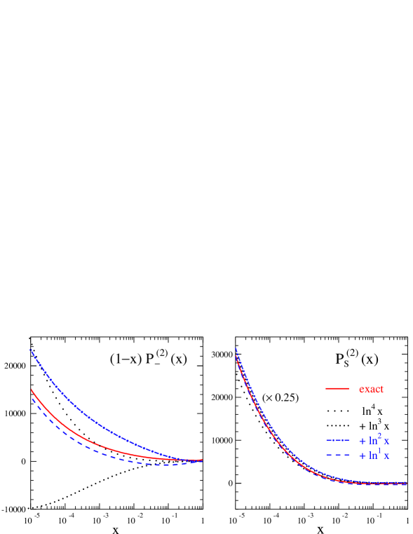
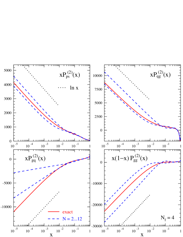
Figure 2: The small-$x$ behaviour of non-singlet (upper row) and singlet NNLO splitting functions for ${n_{\!f}}\!=\!4$. Also shown are the (successive) approximations (4.5) and (4.8) by the leading small-$x$ logarithms and, for the singlet cases, the errors bands [51] used in the analyses of refs. [52, 53].

5 The size of the corrections

Finally we discuss the numerical effects of our new contributions $P^{\,(2)}$ to Eq. (1.3). For brevity, we confine ourselves to four quark flavours and a typical scale $\mu^{2}\simeq 30\ldots 50\mbox{ GeV}^{2}$. We employ an order-independent value of the strong coupling,

$$\alpha_{\rm s}(\mu_{0}^{2},{n_{\!f}}=4)=0.2\>\>,$$ (5.1)

facilitating a direct comparison of the $\overline{\mbox{MS}}$ evolution kernels at LO, NLO and NNLO.

5.1 N-space : anomalous dimensions

The singlet anomalous dimensions $\gamma_{\>\!\rm f\>\!f^{\prime}}$ are displayed in Fig. 3 for the standard choice $\mu_{r}=\mu_{f}$ of the renormalization scale tacitly made already in sections 3 and 4. The NNLO corrections are markedly smaller than the NLO contributions. For the choice (5.1) they amount, at $N\!>\!2$, to less than 2% and 1% for the large diagonal quantities $\gamma_{\>\!\rm qq}$ and $\gamma_{\>\!\rm gg}$, respectively, while for the much smaller off-diagonal anomalous dimensions $\gamma_{\>\!\rm qg}$ and $\gamma_{\>\!\rm gq}$ values of up to 6% and 4% are reached. Also shown in Fig. 3 is the pure-singlet contribution $\gamma_{\>\!\rm ps}$ defined by Eq. (2.8). At $N>2$ this quantity receives very large relative (but tiny absolute) NNLO corrections.

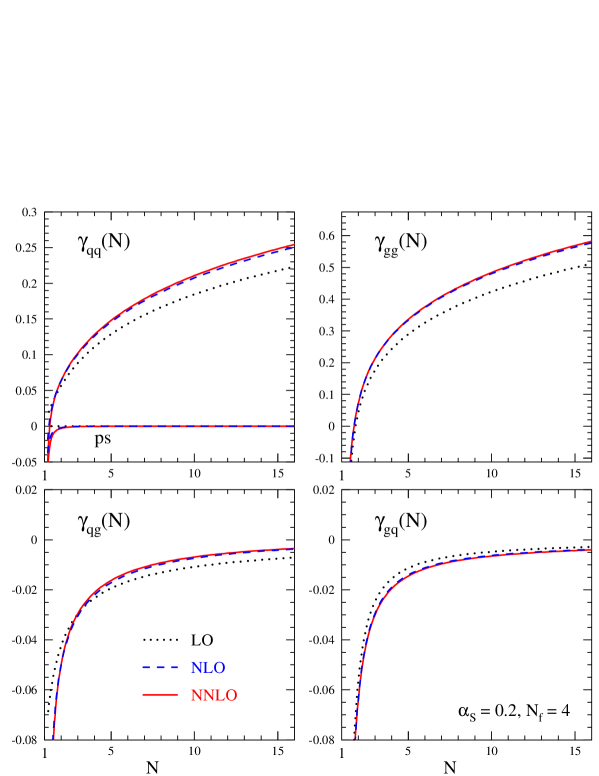
Figure 3: The perturbative expansion of the singlet anomalous dimensions $\gamma_{\rm f\>\!f^{\prime}}$ up to NNLO.

5.2 Scale derivatives of $x$-space parton distributions

In Figs. 4 and 5 we show the logarithmic derivatives $\dot{f_{k}}=d\ln f_{k}/d\ln\mu_{\!f}^{2}$ for the sufficiently realistic – and like Eq. (5.1) order-independent – model distributions

$$xq_{\rm ns}(x,\mu_{0}^{\,2}) \>=\> x^{\,0.5}\,(1-x)^{3}$$

$$xq_{\rm s}(x,\mu_{0}^{\,2})\> \>=\> 0.6\>x^{\,-0.3}\,(1-x)^{3.5}\,(1+5.0\>x^{\,0.8\,})$$

$$xg(x,\mu_{0}^{\,2})\>\> \>=\> 1.6\>x^{\,-0.3}\,(1-x)^{4.5}\,(1-0.6\>x^{\,0.3\,})\>\>.$$ (5.2)

At large $x$ the NNLO corrections to the non-singlet evolution illustrated in Fig. 4 are very similar for all three cases (2.5). They amount to 2% or less for $x\geq 0.2$, thus being smaller than the NLO contributions by a factor of about eight. For $q_{\,\rm ns}^{\,-}$ the same suppression is also found in the region $10^{-5}\raisebox{-1.9919pt}{$\>\stackrel{{\scriptstyle<}}{{{\scriptstyle\sim}}}\>$}x\raisebox{-1.9919pt}{$\>\stackrel{{\scriptstyle<}}{{{\scriptstyle\sim}}}\>$}10^{-2}$. The NNLO effects are even smaller for $q_{\,\rm ns}^{\,+}$ (not shown) at small $x$, but considerably larger for $q_{\,\rm ns}^{\,\rm v}$ at $x<10^{-3}$ due to the additional effect of the new quantity $P_{\rm ns}^{\,\rm s}$ in Eq. (2.2).

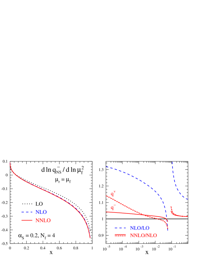
Figure 4: The perturbative expansion up to NNLO of the factorization-scale derivatives $\dot{q}_{\,\rm ns}^{\,-,\rm v}$ for the initial conditions (5.1), (5.2) and the standard choice $\mu_{r}=\mu_{f}$ of the renormalization scale.

Also for the singlet quark distribution (upper row of Fig. 5) the ratio of the NLO and NNLO corrections is about eight over the full $x$-range. However, at small$~{}x$ – where $P_{\rm qg}\ast g$ dominates in Eq. (2.7) – the LO results are anomalously small as $P_{\rm qq}$ and $P_{\rm qg}$, unlike at higher orders, do not include $1/x$ terms at first order. The situation is quite different for the evolution of the gluon density (dominated by $P_{\rm gg}\ast g$ at all $x$). Here the NLO contributions appear atypically small at low $x$, cf. the remark below Eq. (4.8). Thus the ratio of the NNLO and NLO corrections is rather large here, despite the former amounting to only 3% for $x$ as low as $10^{\,-4}$.

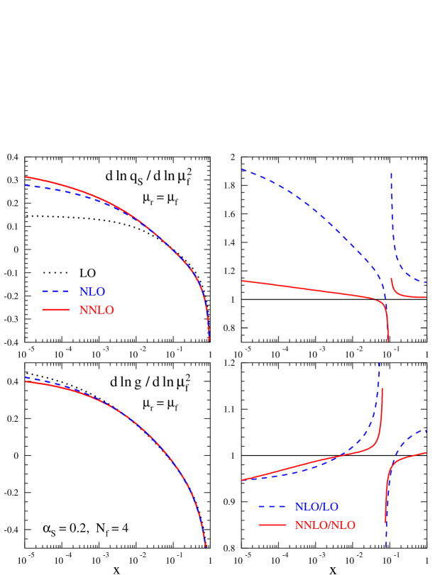
Figure 5: As Fig. 4, but for the singlet quark and gluon distributions $q_{\>\!\rm s}$ and $g$. The spikes close $x=0.1$ in the right plots reflect the zeros of $\dot{f}_{k}$ and do not constitute large absolute corrections.

It is also interesting to consider the stability of the above results under variations of the renormalization scale $\mu_{r}$. For $\mu_{r}\neq\mu_{f}$ the perturbative expansion of the splitting functions up to NNLO reads, with $L_{fr}\,\equiv\,\ln(\mu_{f}^{\,2}/\mu_{r}^{2})$,

$$P \>=\> \quad a_{\rm s}(\mu_{r}^{\,2})\>P^{(0)}\>\>+\>\>a_{\rm s}^{\,2}(\mu_{r}^{\,2})\,\big{(}P^{(1)}-\beta_{0}\,P^{(0)}L_{fr}\big{)}\>$$ (5.3)

$$\mbox{}\!\!\!+\>a_{\rm s}^{\,3}(\mu_{r}^{\,2})\,\big{(}P^{(2)}-\{\beta_{1}P^{(0)}+2\beta_{0}\,P^{(1)}\}L_{fr}+\beta_{0}^{2}\,P^{(0)}L_{fr}^{2}\big{)}\>\>.$$

Here $a_{\rm s}(\mu_{\,r}^{\,2})$ is obtained at NⁿLO from the value (5.1) at the scale $\mu_{0}^{2}$ by solving

$$\frac{da_{\rm s}}{d\ln\mu_{r}^{2}}\>=\>\beta(a_{\rm s})\>=\>-\sum_{l=0}^{n}\,a_{\rm s}^{\,k+2}\beta_{k}\>\>.$$ (5.4)

The $\overline{\mbox{MS}}$ expansion coefficients $\beta_{k}$ are presently known up to $k=3$ [54]–[58].

The dependence of the above results on $\mu_{r}$ can be found in Fig. 8 of ref. [1] and Figs. 9 and 10 of ref. [2] for selected values of $x$. Here we only show, in Fig. 6, the relative scale uncertainties $\Delta\dot{f_{k}}$ of the average $\mu_{f}$-derivatives as conventionally estimated by varying $\mu_{r}$ up to a factor of two with respect to $\mu_{f}$,

$$\Delta\dot{f}\>=\>\frac{\max\,\dot{f}-\min\,\dot{f}}{2\,|\,{\rm average}\,\dot{f}|}\>\>,\quad\mu_{r}^{2}=\frac{1}{4}\,\mu_{\!f}^{2}\ldots\,4\,\mu_{\!f}^{2}\>\>.$$ (5.5)

For the valence, (singlet-quark, gluon) distributions, these uncertainty estimates amount to 3% (3%, 1%) or less at $x>5\cdot 10^{-4\,}$ ($5\cdot 10^{-3\,}$, $3\cdot 10^{-4\,}$), an improvement by more than a factor of three with respect to the corresponding NLO results.

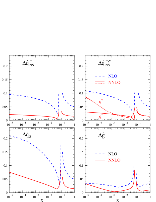
Figure 6: The renormalization scale uncertainties of the NLO and NNLO predictions for the evolution of the non-singlet and singlet distributions as estimated by the quantities $\Delta\dot{f}_{k}$ in Eq. (5.5).

6 Summary and outlook

We have calculated the complete third-order splitting functions for the evolution of unpolarized parton distributions in perturbative QCD. The computation is performed in Mellin-$N$ space and follows the previous fixed-$N$ computations [12]–[14] inasmuch as we compute the partonic structure functions in deep-inelastic scattering at even or odd $N$. Our calculation, however, provides the complete $N$-dependence from which the splitting functions in Bjorken-$x$ space can be uniquely reconstructed.

A salient feature of our approach is that it facilitates very efficient checks of our elaborate schemes for the reduction of the required three-loop integrals by using the Mincer program [24, 25]. By keeping terms of order $\varepsilon^{0}$ in dimensional regularization throughout the calculation, we have also obtained the third-order coefficient functions for the structure functions $F_{2}$ and $F_{L}$ in electromagnetic and for $F_{3}$ in charged-current DIS [23]. The present method can be used to generalize our fixed-$N$ three-loop calculation of the photon structure [59] to all $N$. It should also be possible to obtain the polarized NNLO splitting function in this manner.

Our results completely agree with all partial results available in the literature for fixed moments [12]–[14], large-${n_{\!f}}$ limits [15, 16], small-$x$ behaviour [17]–[19] and large-$x$ structure [22, 44]. With the (relatively unimportant) exception of $P_{\rm gq}$ shown above and $P_{\rm ns}^{\,\rm s}$ they also fully agree with the uncertainty bands of ref. [51] used in provisional NNLO analyses [52, 53]. Those analyses thus remain valid. The results do, however, exhibit some unexpected features, most notably a suggestive relation between large-$x$ coefficients and the presence of a leading small-$x$ term in the new $d_{abc}d_{abc}$ contribution $P_{\rm ns}^{\,\rm s}$ to the splitting function for the valence distribution.

The effect of the three-loop (NNLO) corrections on the evolution of the parton densities is small at $x\raisebox{-1.9919pt}{$\>\stackrel{{\scriptstyle>}}{{{\scriptstyle\sim}}}\>$}10^{-3}$. For $\alpha_{\rm s}=0.2$, for example, both the corrections and the $\mu_{r}$ variation amount to less than 2% at large $x$; and the NNLO effects are about eight times smaller than the NLO contributions, implying that the evolution is perturbatively stable down to rather low scales. For $x\!<\!10^{-3}$ the corrections increase with decreasing $x$. As the knowledge of the leading small-$x$ terms is not sufficient, further improvements in this region would require considerable efforts, including at least an extension of the Mincer program [24, 25] to four loops.

References

- [1] S. Moch, J.A.M. Vermaseren and A. Vogt, Nucl. Phys. B688 (2004) 101, hep-ph/0403192
- [2] A. Vogt, S. Moch and J.A.M. Vermaseren, Nucl. Phys. B691 (2004) 129, hep-ph/0404111
- [3] D.J. Gross and F. Wilczek, Phys. Rev. D8 (1973) 3633
- [4] H. Georgi and H.D. Politzer, Phys. Rev. D9 (1974) 416
- [5] G. Altarelli and G. Parisi, Nucl. Phys. B126 (1977) 298
- [6] E.G. Floratos, D.A. Ross and C.T. Sachrajda, Nucl. Phys. B129 (1977) 66
- [7] E.G. Floratos, D.A. Ross and C.T. Sachrajda, Nucl. Phys. B152 (1979) 493
- [8] G. Curci, W. Furmanski and R. Petronzio, Nucl. Phys. B175 (1980) 27
- [9] W. Furmanski and R. Petronzio, Phys. Lett. 97B (1980) 437
- [10] E.G. Floratos, C. Kounnas and R. Lacaze, Nucl. Phys. B192 (1981) 417
- [11] R. Hamberg and W.L. van Neerven, Nucl. Phys. B379 (1992) 143
- [12] S. Larin, T. van Ritbergen, and J. Vermaseren, Nucl. Phys. B427 (1994) 40
- [13] S. Larin, P. Nogueira, T. van Ritbergen and J. Vermaseren, Nucl. Phys. B492 (1997) 338, hep-ph/9605317
- [14] A. Retey and J. Vermaseren, Nucl. Phys. B604 (2001) 281, hep-ph/0007294
- [15] J.A. Gracey, Phys. Lett. B322 (1994) 141, hep-ph/9401214
- [16] J.F. Bennett and J.A. Gracey, Nucl. Phys. B517 (1998) 241, hep-ph/9710364
- [17] S. Catani and F. Hautmann, Nucl. Phys. B427 (1994) 475, hep-ph/9405388
- [18] J. Blümlein and A. Vogt, Phys. Lett. B370 (1996) 149, hep-ph/9510410
- [19] V.S. Fadin and L.N. Lipatov, Phys. Lett. B429 (1998) 127, hep-ph/9802290
- [20] S. Moch, J.A.M. Vermaseren and A. Vogt, Nucl. Phys. B646 (2002) 181, hep-ph/0209100
- [21] J. Vermaseren, S. Moch and A. Vogt, Nucl. Phys. Proc. Suppl. 116 (2003) 100, hep-ph/0211296
- [22] C.F. Berger, Phys. Rev. D66 (2002) 116002, hep-ph/0209107
- [23] J.A.M. Vermaseren, A. Vogt and S. Moch, in preparation
- [24] S.G. Gorishnii et al., Comput. Phys. Commun. 55 (1989) 381
- [25] S.A. Larin, F.V. Tkachev and J.A.M. Vermaseren, NIKHEF-H-91-18
- [26] S. Larin and J. Vermaseren, Phys. Lett. B259 (1991) 345
- [27] W.L. van Neerven and E.B. Zijlstra, Phys. Lett. B272 (1991) 127
- [28] E.B. Zijlstra and W.L. van Neerven, Phys. Lett. B273 (1991) 476
- [29] E.B. Zijlstra and W.L. van Neerven, Phys. Lett. B297 (1992) 377
- [30] E.B. Zijlstra and W.L. van Neerven, Nucl. Phys. B383 (1992) 525
-
[31]
F.J. Ynduráin, The Theory of Quark and Gluon Interactions, 3rd edition,
(Springer 1999) and references therein. - [32] H. Kluberg-Stern and J.B. Zuber, Phys. Rev. D12 (1975) 467
- [33] J.C. Collins, A. Duncan, and S.D. Joglekar, Phys. Rev. D16 (1977) 438
- [34] P. Nogueira, J. Comput. Phys. 105 (1993) 279
- [35] J.A.M. Vermaseren, math-ph/0010025
- [36] J.A.M. Vermaseren, Nucl. Phys. Proc. Suppl. 116 (2003) 343, hep-ph/0211297
- [37] J.A.M. Vermaseren, Int. J. Mod. Phys. A14 (1999) 2037, hep-ph/9806280
- [38] E. Remiddi and J.A.M. Vermaseren, Int. J. Mod. Phys. A15 (2000) 725, hep-ph/9905237
- [39] S. Moch and J. Vermaseren, Nucl. Phys. B573 (2000) 853, hep-ph/9912355
- [40] T. Gehrmann and E. Remiddi, Comput. Phys. Commun. 141 (2001) 296, hep-ph/0107173
- [41] Ch. Berger, D. Graudenz, M. Hampel and A. Vogt, Z. Phys. C70 (1996) 77, hep-ph/9506333
- [42] D. A. Kosower, Nucl. Phys. B520 (1998) 263, hep-ph/9708392
-
[43]
M. Stratmann and W. Vogelsang,
Phys. Rev. D64 (2001) 114007,
hep-ph/0107064 - [44] G. P. Korchemsky, Mod. Phys. Lett. A4 (1989) 1257
- [45] A. Vogt, Phys. Lett. B497 (2001) 228, hep-ph/0010146
- [46] R. Kirschner and L.N. Lipatov, Nucl. Phys. B213 (1983) 122
- [47] E.A. Kuraev, L.N. Lipatov and V.S. Fadin, Sov. Phys. JETP 45 (1977) 199
- [48] I.I. Balitsky and L.N. Lipatov, Sov. J. Nucl. Phys. 28 (1978) 822
- [49] T. Jaroszewicz, Phys. Lett. B116 (1982) 291.
- [50] W.L. van Neerven and A. Vogt, Nucl. Phys. B588 (2000) 345, hep-ph/0006154
- [51] W.L. van Neerven and A. Vogt, Phys. Lett. B490 (2000) 111, hep-ph/0007362
- [52] A.D. Martin, R.G. Roberts, W.J. Stirling and R.S. Thorne, Phys. Lett. B531 (2002) 216, hep-ph/0201127
- [53] S. Alekhin, Phys. Rev. D68 (2003) 014002, hep-ph/0211096
- [54] W.E. Caswell, Phys. Rev. Lett. 33 (1974) 244
- [55] D.R.T. Jones, Nucl. Phys. B75 (1974) 531
- [56] O.V. Tarasov, A.A. Vladimirov, and A.Y. Zharkov, Phys. Lett. 93B (1980) 429
- [57] S. Larin and J. Vermaseren, Phys. Lett. B303 (1993) 334, hep-ph/9302208
- [58] T. van Ritbergen, J. Vermaseren and S. Larin, Phys. Lett. B400 (1997) 379, hep-ph/9701390
- [59] S. Moch, J.A.M. Vermaseren and A. Vogt, Nucl. Phys. B621 (2002) 413, hep-ph/0110331