IPPP/04/38

DCTP/04/76

HIP-2004-33/TH

CERN-PH-TH/2004-133

Comparative Study of CP Asymmetries

in Supersymmetric Models

E. Gabrielli^a,c, K. Huitu^a,b, and S. Khalil^d,e

^aHelsinki Institute of Physics, P.O.B. 64, 00014 University of Helsinki, Finland
^bDiv. of HEP, Dept. of Phys., P.O.B. 64, 00014 University of Helsinki, Finland

^cCERN PH-TH, Geneva 23, Switzerland
^dIPPP, University of Durham, South Rd., Durham DH1 3LE, U.K.
^eDept. of Math., German University in Cairo - GUC, New Cairo, El Tagamoa Al Khames, Egypt.

We systematically analyze the supersymmetric contributions to the mixing CP asymmetries and branching ratios of $B\to\phi K_{S}$ and $B\to\eta^{\prime}K_{S}$ processes. We consider both gluino and chargino exchanges in a model independent way by using the mass insertion approximation method. While we adopt the QCD factorization approach for evaluating the corresponding hadronic matrix elements, a critical comparison with predictions in naive factorization one is also provided. We find that pure chargino contributions cannot accommodate the current experimental results on CP asymmetries, mainly due to $b\to s\gamma$ constraints. We show that charged Higgs contributions can relax these constraints making chargino responsible for large asymmetries. On the other hand, pure gluino exchanges can easily saturate both the constraints on $B\to\phi K_{S}$ and $B\to\eta^{\prime}K_{S}$ CP asymmetries. Moreover, we also find that the simultaneous contributions from gluino and chargino exchanges could easily account for the present experimental results on the mentioned asymmetries. Remarkably, large experimentally allowed enhancements of $B\to\eta^{\prime}K_{S}$ branching ratio can easily be achieved by the contribution of two mass insertions in gluino exchanges. Finally, we analyze the correlations between the CP asymmetries of these processes and the direct CP asymmetry in $b\to s\gamma$ decay. When all experimental constraints are satisfied, supersymmetry favors large and positive values of $b\to s\gamma$ asymmetry.

1 Introduction

The B-factories are producing interesting experimental results with continuously increasing integrated luminosities. Currently they offer one of the most promising routes to test the Kobayashi-Maskawa ansatz for the CP violation. The understanding of the CP violating mechanism is one of the major open problems in particle physics. There are reasons to believe that the Standard Model (SM) cannot provide a complete description for the CP violating phenomena in nature. For instance, it is established that the SM mechanism of CP violation cannot account for the observed size of the baryon asymmetry in the Universe, and additional sources of CP violation beyond the SM are needed [1].

Recently, BaBar and Belle collaborations [2] announced large deviations from the SM expectations in the CP asymmetry of $B^{0}\to\phi K_{S}$ and branching ratio of $B^{0}\to\eta^{\prime}K^{0}$. These discrepancies have been interpreted as possible consequences of new physics (NP) beyond the SM [3, 4, 5, 6, 7, 8, 9, 10, 11, 12]. For $B^{0}$ and $\bar{B}^{0}$ decays to a CP eigenstate $f_{CP}$, the time dependent CP asymmetries are usually described by rates $a_{f_{CP}}(t)$,

$$a_{f_{CP}}(t)=\frac{\Gamma(\overline{B}^{0}(t)\to f_{CP})-\Gamma(B^{0}(t)\to f_{CP})}{\Gamma(\overline{B}^{0}(t)\to f_{CP})+\Gamma(B^{0}(t)\to f_{CP})}=C_{f_{CP}}\cos\Delta M_{B_{d}}t+S_{f_{CP}}\sin\Delta M_{B_{d}}t,$$ (1)

where $C_{f_{CP}}$ and $S_{f_{CP}}$ represent the parameters of direct and indirect CP violations respectively, and $\Delta M_{B_{d}}$ is the $B^{0}$ eigenstate mass difference.

In the Standard Model, the angle $\beta$ in the unitary triangle of Cabibbo-Kobayashi-Maskawa (CKM) matrix [13], can be measured from $B$ meson decays. The golden mode $B^{0}\to J/\psi K_{S}$ is dominated by tree contribution and $S_{J/\psi K_{S}}=\sin 2\beta+{\cal{O}}(\lambda^{3})$, where $\lambda$ is the Cabibbo mixing angle (see e.g. [14]). These uncertainties are less than 1%.

The dominant part of the decay amplitudes for $B^{0}\to\phi K_{S},\;\eta^{\prime}K_{S}$ is assumed to come from the gluonic penguin [15, 16], but some contribution from the tree level $b\to u\bar{u}s$ decay is expected. The $|\phi\rangle$ is almost pure $|s\bar{s}\rangle$ and consequently this decay mode corresponds also accurately, up to terms of orders ${\cal{O}}(\lambda^{2})$, to $\sin 2\beta$ in the SM [17]. The $b\to u\bar{u}s$ tree level contribution to $B_{d}\to\eta^{\prime}K$ was estimated in [16]. It was found that the tree level amplitude is less than 2% of the gluonic penguin amplitude. Thus also in this mode one measures the angle $\beta$ with a good precision in the SM. Therefore, it is expected that NP contributions to the CP asymmetries in $B^{0}\to\phi K_{S},\;\eta^{\prime}K_{S}$ decays are more significant than in $B^{0}\to J/\psi K_{S}$ and can compete with the SM one.

New sample of data have been recently analyzed by BaBar and Belle collaboration and the results with higher statistics have been now announced in [18, 19]. The new experimental value of the indirect CP asymmetry parameter for $B^{0}\to J/\psi K_{S}$ is given by [18, 19]

$$S_{J/\psi K_{S}}=0.726\pm 0.037,$$ (2)

which does not differ much from the previous one [20, 21], and agrees quite well with the SM prediction $0.715_{-0.045}^{+0.055}$ [22]. However, results of Belle on the corresponding $\sin{2\beta}$ extracted for $B^{0}\to\phi K_{S}$ process has changed dramatically [18, 19]

$$S_{\phi K_{S}} = 0.50\pm 0.25^{+0.07}_{-0.04}\;\;({\rm BaBar}),$$ (3)

$$= 0.06\pm 0.33\pm 0.09\;\;({\rm Belle})\,,$$

where the first errors are statistical and the second systematic, showing now a better agreement than before [23, 24]. However, as we can see from Eq.(3), the relative central values are still different. BaBar results [18] are more compatible with SM predictions, while Belle measurements [19] still show a deviation from the $c\bar{c}$ measurements of about $2\sigma$. Moreover, the average $S_{\phi K_{S}}=0.34\pm 0.20$ is quite different from the previous one [25], displaying now 1.7$\sigma$ deviation from Eq.(2).

Furthermore, the most recent measured CP asymmetry in the $B^{0}\to\eta^{\prime}K_{S}$ decay is found by BaBar [18] and Belle [19] collaborations as

$$S_{\eta^{\prime}K_{S}} = 0.27\pm 0.14\pm 0.03\;\;({\rm BaBar})$$ (4)

$$= 0.65\pm 0.18\pm 0.04\;\;({\rm Belle}),$$

with an average $S_{\eta^{\prime}K_{S}}=0.41\pm 0.11$, which shows a 2.5$\sigma$ discrepancy from Eq. (2). For the previous results see (BaBar) [26] and (Belle) [24].

It is interesting to note that the new results on s-penguin modes from both experiments differ from the value extracted from the $c\bar{c}$ mode ($J/\psi$), BaBar by 2.7$\sigma$ and Belle by 2.4$\sigma$ [18, 19]. At the same time the experiments agree with each other, and even the central values are quite close:

$$0.42\pm 0.10\;\;{\rm BaBar},\;\;\;0.43^{+0.12}_{-0.11}\;\;{\rm Belle}.$$

On the other hand, the experimental measurements of the branching ratios of $B^{0}\to\phi K^{0}$ and $B^{0}\to\eta^{\prime}K^{0}$ at BaBar [27], Belle [28], and CLEO [29] lead to the following averaged results [25] :

$$BR(B^{0}\to\phi K^{0}) = (8.3^{+1.2}_{-1.0})\times 10^{-6},$$ (5)

$$BR(B^{0}\to\eta^{\prime}K^{0}) = (65.2^{+6.0}_{-5.9})\times 10^{-6}.$$ (6)

From theoretical side, the SM predictions for $BR(B\to\phi K)$ are in good agreement with Eq.(5), while showing a large discrepancy, being experimentally two to five times larger, for $BR(B\to\eta^{\prime}K)$ in Eq.(6) [30]. This discrepancy is not new and it has created a growing interest in the subject. However, since it is observed only in $B\to\eta^{\prime}K$ process, mechanisms based on the peculiar structure of $\eta^{\prime}$ meson, such as intrinsic charm [31] and gluonium [32] content, have been investigated to solve the puzzle.

Supersymmetry (SUSY) is one of the most popular candidates for physics beyond the SM [33]. In SUSY models there are new sources of CP violation besides the CKM phase [34]. The soft SUSY breaking (SSB) terms contain several parameters that may be complex, as may also be the SUSY preserving $\mu$ parameter in the Higgs sector. Then, new CP violating phases can naturally arise in the SSB sector of scalar- quarks (squarks) and -leptons (sleptons). These new phases have significant implications for the electric dipole moments (EDM) of the neutron, electron, and mercury atom [34, 35] and can be strongly constrained by the negative search of CP violation in EDM experiments. Therefore, it remains a challenge for SUSY to provide an explanation for the above mentioned discrepancies in $B$-decays, while keeping the above EDMs within their experimental ranges. This can be possible, for instance, in SUSY models where the CP violating phases entering in $b\to s$ transitions are independent from the corresponding ones affecting EDMs. An interesting example is provided by SUSY models with flavor dependent CP violating phases [35, 36, 37].

In SUSY framework, the main effect on $B\to\phi K$ is usually assumed to come from the gluino loop contributions to s-penguin diagrams [38, 6, 7, 9, 8], if R parity is conserved. However, charginos could also be responsible for such discrepancy, as it has been discussed in [10, 11], although $b\to s\gamma$ constraints strongly suppress their contribution [11]. Similarly to $B\to\phi K$, one would a priori expect large effects from SUSY corrections to $B\to\eta^{\prime}K$ as well, which may contradict the experimental results reported in Eq.(4). Possible mechanisms to explain such behavior in the supersymmetric context have been proposed in Refs.[9, 8, 39].

In this paper we perform a complete analysis of SUSY contributions to the CP asymmetries and branching ratios of $B\to\phi K$ and $B\to\eta^{\prime}K$ processes. Previous analyses on the same issue have considered either gluino [6] or chargino exchanges [11, 10, 7]. We think that in the framework of general SUSY models a complete analysis involving both effects is in fact needed. Indeed, we find that a SUSY scenario in which both chargino and gluino give sizeable contributions to CP violating processes, is an interesting viable possibility. For instance, large effects of chargino contributions to CP asymmetries that one would expect to be excluded by $b\to s\gamma~{}$constraints [11], could be achieved taking into account gluino exchanges. This is due to potentially destructive interferences between chargino and gluino amplitudes in $b\to s\gamma$ decay that eventually relax $b\to s\gamma$ bounds.

In our analysis we consider both the effects of gluino and chargino exchanges by using the mass insertion method (MIA) [40]. As known, this method is a useful tool for analyzing SUSY contributions to flavor changing neutral current processes (FCNC) since it allows to parametrize, in a model independent way, the main sources of flavor violations in general SUSY models.

We take into account all the relevant operators involved in the effective Hamiltonian for $\Delta B=1$ transition, and provide analytical expression for the corresponding Wilson coefficients. We analyze the most interesting scenarios in which one or two mass insertions are dominant in both gluino and chargino sector.

An important issue in these calculations is the method of evaluating the hadronic matrix elements for exclusive hadronic final states, which may play a crucial role in CP asymmetries. Many studies have been done with naive factorization approach (NF) [41, 42], for the computation of two-body nonleptonic B decays. Recently, a new approach has been developed, called QCD factorization (QCDF), [43, 44, 45], which offers the possibility to include non-factorizable contributions and to calculate the strong phases. The drawback in this approach is that it includes undetermined parameters $\rho_{H,A}$ and phases $\phi_{H,A}$, characterizing the infrared divergences. We critically consider both approaches and analyze theoretical uncertainties connected with SUSY predictions. We provide a comparative study of SUSY contributions from chargino and gluino to $B\rightarrow\phi K$ and $B\rightarrow\eta^{\prime}K$ processes in NF and QCDF approaches. We also analyze the branching ratios of these decays and investigate their correlations with CP asymmetries. Finally, we discuss the correlations between CP asymmetries of these processes and the direct CP asymmetry in $b\to s\gamma$ decay [46].

This paper is organized as follows. In Section 2 we give the basic ingredients needed for calculations, with many important formulas provided in the Appendices. In Section 3 we discuss the QCDF method in the evaluation of $B$-meson decay amplitudes of $B\to\phi K$ and $B\to\eta^{\prime}K$. Moreover, we compare SUSY predictions between NF and QCDF approaches. Section 4 is devoted to the CP asymmetries of these decay modes. Both effects from gluino and chargino exchanges are discussed. In section 5 the branching ratios and their correlations to asymmetries are considered. Section 6 contains the analysis of SUSY contributions to direct $b\to s\gamma$ asymmetry, and correlations to the mentioned CP asymmetries are also considered. Finally, section 7 contains our main conclusions.

2 SUSY contributions to the effective Hamiltonian of $\Delta B=1$ transitions

We start our analysis by considering the supersymmetric effect in the non-leptonic $\Delta B=1$ processes. Such an effect could be a probe for any testable SUSY implications in CP violating experiments. The most general effective Hamiltonian $H^{\Delta B=1}_{\rm eff}$ for these processes can be expressed via the Operator Product Expansion (OPE) as [47]

$$H^{\Delta B=1}_{\rm eff} = \left\{\frac{G_{F}}{\sqrt{2}}\sum_{p=u,c}\lambda_{p}~{}\left(C_{1}Q_{1}^{p}+C_{2}Q_{2}^{p}+\sum_{i=3}^{10}C_{i}Q_{i}+C_{7\gamma}Q_{7\gamma}+C_{8g}Q_{8g}\right)\right\}$$ (7)

$$+ \left\{Q_{i}\to\tilde{Q}_{i}\,,\,C_{i}\to\tilde{C}_{i}\right\}\;,$$

where $\lambda_{p}=V_{pb}V^{\star}_{ps}$, with $V_{pb}$ the unitary CKM matrix elements satisfying the unitarity triangle relation $\lambda_{t}+\lambda_{u}+\lambda_{c}=0$, and $C_{i}\equiv C_{i}(\mu_{b})$ are the Wilson coefficients at low energy scale $\mu_{b}\simeq{\cal O}(m_{b})$. The basis $Q_{i}\equiv Q_{i}(\mu_{b})$ is given by the relevant local operators renormalized at the same scale $\mu_{b}$, namely

$$Q^{p}_{2} = (\bar{p}b)_{V-A}~{}~{}(\bar{s}p)_{V-A}\;,~{}~{}~{}~{}~{}~{}~{}~{}~{}~{}~{}~{}~{}~{}~{}Q^{p}_{1}=(\bar{p}_{\alpha}b_{\beta})_{V-A}~{}~{}(\bar{s}_{\beta}p_{\alpha})_{V-A}\;$$

$$Q_{3} = (\bar{s}b)_{V-A}~{}~{}\sum_{q}(\bar{q}q)_{V-A}\;,~{}~{}~{}~{}~{}~{}~{}~{}~{}~{}~{}Q_{4}=(\bar{s}_{\alpha}b_{\beta})_{V-A}~{}~{}\sum_{q}(\bar{q}_{\beta}q_{\alpha})_{V-A}\;,$$

$$Q_{5} = (\bar{s}b)_{V-A}~{}~{}\sum_{q}(\bar{q}q)_{V+A}\;,~{}~{}~{}~{}~{}~{}~{}~{}~{}~{}~{}Q_{6}=(\bar{s}_{\alpha}b_{\beta})_{V-A}~{}~{}\sum_{q}(\bar{q}_{\beta}q_{\alpha})_{V+A}\;,$$

$$Q_{7} = (\bar{s}b)_{V-A}~{}~{}\sum_{q}\frac{3}{2}e_{q}(\bar{q}q)_{V+A}\;,~{}~{}~{}~{}~{}~{}Q_{8}=(\bar{s}_{\alpha}b_{\beta})_{V-A}~{}~{}\sum_{q}\frac{3}{2}e_{q}(\bar{q}_{\beta}q_{\alpha})_{V+A}\;,$$

$$Q_{9} = (\bar{s}b)_{V-A}~{}~{}\sum_{q}\frac{3}{2}e_{q}(\bar{q}q)_{V-A}\;,~{}~{}~{}~{}~{}~{}Q_{10}=(\bar{s}_{\alpha}b_{\beta})_{V-A}~{}~{}\sum_{q}\frac{3}{2}e_{q}(\bar{q}_{\beta}q_{\alpha})_{V-A}\;,$$

$$Q_{7\gamma} = \frac{e}{8\pi^{2}}m_{b}\bar{s}\sigma^{\mu\nu}(1+\gamma_{5})F_{\mu\nu}b\;,~{}~{}~{}~{}~{}~{}~{}Q_{8g}=\frac{g_{s}}{8\pi^{2}}m_{b}\bar{s}_{\alpha}\sigma^{\mu\nu}(1+\gamma_{5})G^{A}_{\mu\nu}t^{A}_{\alpha\beta}b_{\beta}\;.$$ (8)

Here $\alpha$ and $\beta$ stand for color indices, and $t^{A}_{\alpha\beta}$ the $SU(3)_{c}$ color matrices, $\sigma^{\mu\nu}=\frac{1}{2}i[\gamma^{\mu},\gamma^{\nu}]$. Moreover, $e_{q}$ are quark electric charges in unity of $e$, $(\bar{q}q)_{V\pm A}\equiv\bar{q}\gamma_{\mu}(1\pm\gamma_{5})q$, and $q$ runs over $u$, $d$, $s$, $c$, and $b$ quark labels. In the SM only the first part of right hand side of Eq.(7) (inside first curly brackets) containing operators $Q_{i}$ will contribute, where $Q^{p}_{1,2}$ refer to the current-current operators, $Q_{3-6}$ to the QCD penguin operators, and $Q_{7-10}$ to the electroweak penguin operators, while $Q_{7\gamma}$ and $Q_{8g}$ are the magnetic and the chromo-magnetic dipole operators, respectively. In addition, operators $\tilde{Q}_{i}\equiv\tilde{Q}_{i}(\mu_{b})$ are obtained from $Q_{i}$ by the chirality exchange $(\bar{q}_{1}q_{2})_{V\pm A}\to(\bar{q}_{1}q_{2})_{V\mp A}$. Notice that in the SM the coefficients $\tilde{C}_{i}$ identically vanish due to the V-A structure of charged weak currents, while in MSSM they can receive contributions from both chargino and gluino exchanges [48, 49].

Due to the asymptotic freedom of QCD, the calculation of hadronic weak decay amplitudes can be factorized by the product of long and short distance contributions. The first ones, that will be analyzed in the next section, are related to the evaluation of hadronic matrix elements of $Q_{i}$ and contain the main uncertainty of our predictions. On the other hand, the latter are contained in the Wilson coefficients $C_{i}$ and they can be evaluated in perturbation theory with high precision [47]. For instance, all the relevant contributions of particle spectra above the W mass ($m_{W}$) scale, including SUSY particle exchanges, will enter in $C_{i}(\mu_{W})$ at $\mu_{W}\simeq\mathcal{O}(m_{W})$ scale.

The low energy coefficients $C_{i}(\mu_{b})$ can be extrapolated from the high energy ones $C_{i}(\mu_{W})$ by solving the renormalization group equations for QCD and QED in the SM. The solution is generally expressed as follows [47]

$$C_{i}(\mu)=\sum_{j}\hat{U}_{ij}(\mu,\mu_{W})\,C_{j}(\mu_{W}),$$ (9)

where $\hat{U}_{ij}(\mu,\mu_{W})$ is the evolution matrix which takes into account the re-summation of the terms proportional to large logs $(\alpha_{s}(\mu_{W})\log(\mu_{W}/\mu_{b}))^{n}$ (leading), $(\alpha_{s}^{2}(\mu_{W})\log(\mu_{W}/\mu_{b}))^{n}$ (next-to-leading), etc., in QCD.

In our analysis we include the next-to-leading order (NLO) corrections in QCD and QED for the Wilson coefficients $C_{i=1-10}$ as given in Ref. [47], while for $C_{7\gamma}(\mu)$ and $C_{8g}(\mu)$ we include only the leading order (LO) ones. The expressions for the evolution matrix $\hat{U}_{ij}(\mu,\mu_{W})$ at NLO in QCD and QED can be found in Ref.[47]. The reason for retaining only the LO accuracy in $C_{7\gamma}(\mu)$ $C_{8g}(\mu)$ is that the matrix elements of the dipole operators enter the decay amplitudes only at the NLO [43].

Next we discuss the SUSY contributions to the effective Hamiltonian in Eq.(7). The modifications caused by supersymmetry appear only in the boundary conditions of the Wilson coefficients at $\mu_{W}$ scale and they can be computed through the appropriate matching with one-loop Feynman diagrams where Higgs, neutralino, gluino, and chargino are exchanged, see for instance Refs.[48, 51, 49]. Only chargino and gluino contributions can provide a potential source of new CP violating phase in MSSM and could account for the observed large deviations in $B\to\phi K_{S}$ asymmetry. In principle, the neutralino exchange diagrams involve the same mass insertions as the gluino ones, but they are strongly suppressed compared to the latter. For these reasons we neglect neutralino in our analysis. The charged Higgs contributions cannot generate any new source of CP violation in addition to the SM one, or any sizeable effect to operators beyond the SM basis $Q_{i}$. However, when charged Higgs contributions are taken into account together with chargino or gluino exchanges, their effect is relevant. In particular, as we will show in the next sections, due to destructive interferences with chargino and gluino amplitudes, $b\to s\gamma$ constraints can be relaxed allowing sizeable contributions to the the CP asymmetries.

The results for Wilson coefficients at $\mu_{W}$ scale can be expressed as follows

$$C_{i}(\mu_{W})=C_{i}^{W}+C_{i}^{H}+\lambda_{t}^{-1}\left\{C_{i}^{{\chi}}+C_{i}^{{\tilde{g}}}\right\}$$ (10)

where $C_{i}^{W}$, $C_{i}^{H}$, $C_{i}^{\chi}$, and $C_{i}^{\tilde{g}}$ correspond to the $W$, charged Higgs, chargino, and gluino exchanges respectively. In our analysis we will impose the boundary conditions for $C_{i}^{\chi}$, and $C_{i}^{\tilde{g}}$ at the scale $\mu_{W}=m_{W}$, although they should apply to the energy scale at which SUSY particles are integrated out, namely $M_{S}$. However, these threshold corrections, originating from the mismatch of energy scales, are numerically not significant since the running of $\alpha_{s}$ from $M_{S}$ to $m_{W}$ is not very steep.

Finally, for NDR renormalization scheme, the electroweak contributions to the Wilson coefficients are given by [48, 51]

$$C_{1}^{W} = \frac{14\alpha_{s}}{16\pi},$$

$$C_{2}^{W} = 1-\frac{11}{6}\frac{\alpha_{s}}{4\pi},$$

$$C_{3}^{(W,H,\chi)} = \frac{\alpha}{6\pi}\frac{1}{\sin^{2}\theta_{w}}\left(B_{d}^{(W,H,\chi)}+\frac{1}{2}B_{u}^{(W,H,\chi)}+C^{(W,H,\chi)}\right)-\frac{\alpha_{s}}{24\pi}E^{(W,H,\chi)},$$

$$C_{4}^{(W,H,\chi)} = \frac{\alpha_{s}}{8\pi}E^{(W,H,\chi)},$$

$$C_{5}^{(W,H,\chi)} = -\frac{\alpha_{s}}{24\pi}E^{(W,H,\chi)},$$

$$C_{6}^{(W,H,\chi)} = \frac{\alpha_{s}}{8\pi}E^{(W,H,\chi)},$$

$$C_{7}^{(W,H,\chi)} = \frac{\alpha}{6\pi}\left(4C^{(W,H,\chi)}+D^{(W,H,\chi)}\right),$$

$$C_{8}^{(W,H,\chi)} = 0,$$

$$C_{9}^{(W,H,\chi)} = \frac{\alpha}{6\pi}\left(4C^{(W,H,\chi)}+D^{(W,H,\chi)}+\frac{1}{\sin^{2}\theta_{w}}\left(-B_{d}^{(W,H,\chi)}+B_{u}^{(W,H,\chi)}-4C^{(W,H,\chi)}\right)\right),$$

$$C_{10}^{(W,H,\chi)} = 0,$$

$$C_{7\gamma}^{(W,H,\chi)} = M_{\gamma}^{(W,H,\chi)},$$

$$C_{8g}^{(W,H,\chi)} = M_{g}^{(W,H,\chi)}$$ (11)

where $\alpha_{s}$ and $\alpha$ are evaluated at $m_{W}$ scale. The functions appearing above, include the contributions from photon-penguins ($D$), $Z$-penguins ($C$), gluon-penguins ($E$), boxes with external down quarks ($B_{d}$) and up-quarks $(B_{u})$, the magnetic- ($M_{\gamma}$), and the chromo-magnetic-penguins ($M_{g}$). The corresponding SM results are [47] $D^{W}\equiv{\rm D}(x_{t})$, $C^{W}\equiv{\rm C}(x_{t})$, $E^{W}\equiv{\rm E}(x_{t})$, and $B^{W}\equiv{\rm B}(x_{t})$ with $x_{t}=m_{t}^{2}/m_{W}^{2}$, and analogously for charged Higgs [51], $D^{H}\equiv{\rm D_{H}}(x_{H})$, $C^{H}\equiv{\rm C_{H}}(x_{H})$, $E^{H}\equiv{\rm E_{H}}(x_{H})$, and $B^{H}\equiv{\rm B_{H}}(x_{H})$ with $x_{H}=m_{t}^{2}/m_{H}^{2}$, where the loop functions ${\rm B,C,D,E}$ and ${\rm B_{H},C_{H},D_{H},E_{H}}$ and are provided in Appendix C. Regarding the SM and charged Higgs contributions to magnetic-penguins, we have [48]

$$M_{\gamma}^{W} = -x_{t}\left(F_{1}(x_{t})+\frac{3}{2}F_{2}(x_{t})\right),~{}~{}~{}~{}~{}M_{g}^{W}=-\frac{3}{2}x_{t}F_{1}(x_{t})$$

$$M_{\gamma}^{H} = -\frac{x_{H}}{2}\left(\left(\frac{2}{3}F_{1}(x_{H})+F_{2}(x_{H})\right)\cot^{2}{\beta}+\frac{2}{3}F_{3}(x_{H})+F_{4}(x_{H})\right)$$

$$M_{g}^{H} = -\frac{x_{H}}{2}\left(F_{1}(x_{H})\cot^{2}{\beta}+F_{3}(x_{H})\right)\,,$$

where the functions $F_{i}(x)$ are reported in Appendix C. Finally, the gluino and chargino exact contributions to the expressions appearing in Eq.(11) can be found in Refs.[48, 51], while here we will provide only the corresponding results in the so called mass insertion approximation.

Regarding the SUSY contributions to the opposite chirality operators $\tilde{Q}_{i}$, we stress that while in the SM the Wilson coefficients $\tilde{C}_{i}$ identically vanish, in SUSY models chargino and gluino exchanges could sizeably affect these coefficients. However, in case of charginos, these effects are quite small being proportional to the Yukawa couplings of light quarks [11] and so we will not include them in our analysis. Moreover, we have also neglected the small contributions to $C_{1,2}^{\chi}$ coming from box diagrams, where both chargino and gluino are exchanged [11, 51].

As mentioned in the introduction, in order to perform a model independent analysis of FCNC processes in general SUSY models, it is very convenient to adopt the mass insertion approximation (MIA) method [40]. This method has been applied in many analyses of FCNC processes in $K$, $D$, and $B$ meson sector and leptonic sector, mediated by gluino and neutralino exchanges, respectively [40]. More recently, it has been extended to the sector of FCNC processes mediated by chargino exchanges [11, 52, 53]. In particular, in [11], the chargino functions appearing in Eq.(11) have been calculated at the first order in MIA.

Let us briefly recall the main steps of this approximation. In MIA framework, one chooses a basis (called super-CKM basis) where the couplings of fermions and sfermions to neutral gaugino fields are flavor diagonal. In this basis, the interacting Lagrangian involving charginos is given by

$$\mathcal{L}_{q\tilde{q}\tilde{\chi}^{+}} = -g~{}\sum_{k}\sum_{a,b}~{}\Big{(}~{}V_{k1}~{}K_{ba}^{*}~{}\bar{d}_{L}^{a}~{}(\tilde{\chi}^{+}_{k})^{*}~{}\tilde{u}^{b}_{L}-U_{k2}^{*}~{}(Y_{d}^{\mathrm{diag}}.K^{+})_{ab}~{}\bar{d}_{R}^{a}~{}(\tilde{\chi}^{+}_{k})^{*}~{}\tilde{u}^{b}_{L}$$ (12)

$$-V_{k2}~{}(K.Y_{u}^{\mathrm{diag}})_{ab}~{}\bar{d}_{L}^{a}~{}(\tilde{\chi}^{+}_{k})^{*}~{}\tilde{u}^{b}_{R}~{}\Big{)},$$

where $q_{R,L}=\frac{1}{2}(1\pm\gamma_{5})q$, and contraction of color and Dirac indices is understood. Here $Y_{u,d}^{\mathrm{diag}}$ are the diagonal Yukawa matrices, and $K$ stands for the CKM matrix. The indices $a,b$ and $k$ label flavor and chargino mass eigenstates, respectively, and $V$, $U$ are the chargino mixing matrices defined by

$$U^{*}M_{\tilde{\chi}^{+}}V^{-1}=\mathrm{diag}(m_{\tilde{\chi}_{1}^{+}},m_{\tilde{\chi}_{2}^{+}}),~{}\mathrm{and}~{}M_{\tilde{\chi}^{+}}=\left(\begin{array}[]{cc}M_{2}&\sqrt{2}m_{W}\sin\beta\\ \sqrt{2}m_{W}\cos\beta&\mu\end{array}\right)\;,$$ (13)

where $M_{2}$ is the weak gaugino mass, $\mu$ is the supersymmetric Higgs mixing term, and $\tan\beta$ is the ratio of the vacuum expectation value (VEV) of the up-type Higgs to the VEV of the down-type Higgs . As one can see from Eq.(12), the higgsino couplings are suppressed by Yukawas of the light quarks, and therefore they are negligible, except for the stop–bottom interaction which is directly enhanced by the top Yukawa ($Y_{t}$). In our analysis we neglect the higgsino contributions proportional to the Yukawa couplings of light quarks with the exception of the bottom Yukawa $Y_{b}$, since its effect could be enhanced by large $\tan{\beta}$. However, it is easy to show that this vertex cannot affect dimension six operators of the effective Hamiltonian for $\Delta B=1$ transitions (operators $Q_{i=1-10}$ in Eq.(7)) and only interactions involving left down quarks will contribute. On the contrary, contributions proportional to bottom Yukawa $Y_{b}$ enter in the Wilson coefficients of dipole operators ($C_{7\gamma}$, $C_{8g}$) due to the chirality flip of $b\to s\gamma$ and $b\to sg$ transitions.

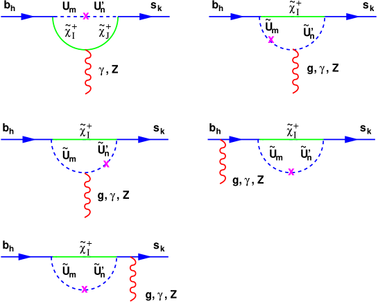
Figure 1: Penguin diagrams for $\Delta B=1$ transitions with chargino ($\chi_{\rm I}^{+}$) exchanges at the first order in mass insertion. Here $\tilde{U},\tilde{U}^{\prime}=\{\tilde{u},\tilde{c},\tilde{t}\}$, with indices $h,k,m,n=\{L,R\}$ and ${\rm I,J}=\{1,2\}$. The cross symbol in the squark propagator indicates the mass insertion. The corresponding diagrams at zero order in mass insertion are simply obtained by removing the mass insertion in the propagators of up-type squarks ($\tilde{U}$).

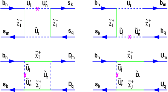
Figure 2: Box diagrams for $\Delta B=1$ transitions with chargino exchanges at the first order in mass insertion, where $\tilde{U},\tilde{U}^{\prime}=\{\tilde{t},\tilde{c},\tilde{u}\}$, $U=\{c,u\}$, and $D=\{b,s,d\}$, where $h,k,l,n,r,m,q=\{L,R\}$.

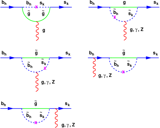
Figure 3: Penguin diagrams for $\Delta B=1$ transitions with gluino exchanges at the first order in mass insertion, where $h,k=\{L,R\}$.

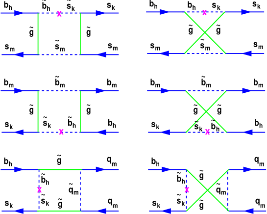
Figure 4: Box diagrams for $\Delta B=1$ transitions with gluino exchanges at the first order in mass insertion, where $q=\{b,c,s,d,u\}$ and $h,k,m=\{L,R\}$.

As mentioned in the case of MIA, the flavor mixing is displayed by the non–diagonal entries of the sfermion mass matrices. Denoting by $\Delta^{q}_{AB}$ the off–diagonal terms in the sfermion $(\tilde{q}=\tilde{u},\tilde{d})$ mass matrices for the up and down, respectively, where $A,B$ indicate chirality couplings to fermions $A,B=(L,R)$, the A–B squark propagator can be expanded as

$$\langle\tilde{q}^{a}_{A}\tilde{q}^{b*}_{B}\rangle=i\left(k^{2}{\bf 1}-\tilde{m}^{2}{\bf 1}-\Delta_{AB}^{q}\right)^{-1}_{ab}\simeq\frac{i\delta_{ab}}{k^{2}-\tilde{m}^{2}}+~{}\frac{i(\Delta_{AB}^{q})_{ab}}{(k^{2}-\tilde{m}^{2})^{2}}+{\cal O}(\Delta^{2}),$$ (14)

where $q=u,d$ selects up or down sector, respectively, $a,b=(1,2,3)$ are flavor indices, ${\bf 1}$ is the unit matrix, and $\tilde{m}$ is the average squark mass. As we will see in the following, it is convenient to parametrize this expansion in terms of the dimensionless quantity $(\delta_{AB}^{q})_{ab}\equiv(\Delta^{q}_{AB})_{ab}/\tilde{m}^{2}$. At the first order in MIA, the penguin and box diagrams which contribute to the $\Delta B=1$ effective Hamiltonian are given in Figs. 1 and 2, respectively. Evaluating the diagrams in Figs. 1 and 2 by retaining only terms proportional to bottom- and top-quark Yukawa couplings and performing the matching, the chargino contributions to the Wilson coefficients in Eqs.(11) can be determined from the following relations [11]

$$F^{\chi}\! =\! \Big{[}\sum_{a,b}K^{\star}_{a2}K_{b3}{\left(\delta^{u}_{LL}\right)_{ba}}\Big{]}R_{F}^{LL}+\Big{[}\sum_{a}K^{\star}_{a2}K_{33}{\left(\delta^{u}_{RL}\right)_{3a}}\Big{]}Y_{t}\,R_{F}^{RL}$$ (15)

$$+ \Big{[}\sum_{a}K^{\star}_{32}K_{a3}{\left(\delta^{u}_{LR}\right)_{a3}}\Big{]}Y_{t}\,R_{F}^{LR}+\Big{[}K^{\star}_{32}K_{33}\left({\left(\delta^{u}_{RR}\right)_{33}}R_{F}^{RR}+R_{F}^{0}\right)\Big{]}Y_{t}^{2}\,,$$

where the symbol $F\equiv\left\{D,C,E,B_{d},B_{u},M_{\gamma},M_{g}\right\}$, and the detailed expressions for $R_{F}^{LL}$, $R_{F}^{LR}$, $R_{F}^{RL}$, $R_{F}^{RR}$, and $R_{F}^{0}$ can be found in Appendix A . Notice that the last term in Eq.(15), proportional to $R_{F}^{0}$, is independent of mass insertions. This is due to the fact that for chargino exchanges the super-GIM mechanism is only partially effective, when only squarks but not quarks are taken to be degenerate.

Here we will just concentrate on the dominant contributions which turn out to be due to the chromo-magnetic ($M_{g}$) penguin and $Z$-penguin ($C$) diagrams [11]. From the above expressions, it is clear that $LR$ and $RR$ contributions are suppressed by order $\lambda^{2}$ or $\lambda^{3}$, where $\lambda=\sin{\theta_{c}}\simeq 0.22$, with $\theta_{c}$ the Cabibbo angle. In our analysis we adopt the approximation of retaining only terms proportional to order $\lambda=\sin{\theta_{c}}$. In this case, Eq.(15) simplifies as follows [11]

$$F^{\chi}=\xi_{LL}R_{F}^{LL}+Y_{t}\,\xi_{RL}R_{F}^{RL}\,,$$ (16)

where $\xi_{LL}={\left(\delta^{u}_{LL}\right)_{32}}+\lambda\,{\left(\delta^{u}_{LL}\right)_{31}}$ and $\xi_{RL}={\left(\delta^{u}_{RL}\right)_{32}}+\lambda\,{\left(\delta^{u}_{RL}\right)_{31}}$.

The functions $R^{LL}_{F}$ and $R^{RL}_{F}$ depend on the SUSY parameters through the chargino masses ($m_{\chi_{i}}$), squark masses ($\tilde{m}$) and the entries of the chargino mass matrix. For instance for $Z$ and magnetic (chromo-magnetic) dipole penguins $R_{C}^{LL,RL}$ and $R_{M_{\gamma(g)}}^{LL,RL}$, respectively, we have

$$R_{C}^{LL} = \sum_{i=1,2}|V_{i1}|^{2}\,P_{C}^{(0)}(\bar{x}_{i})+\sum_{i,j=1,2}\left[U_{i1}V_{i1}U_{j1}^{\star}V_{j1}^{\star}\,P_{C}^{(2)}(x_{i},x_{j})\right.$$

$$+\left.|V_{i1}|^{2}|V_{j1}|^{2}\left(\frac{1}{8}-P_{C}^{(1)}(x_{i},x_{j})\right)\right],$$

$$R_{C}^{RL} = -\frac{1}{2}\sum_{i=1,2}\,V_{i2}^{\star}V_{i1}\,P_{C}^{(0)}(\bar{x}_{i})-\sum_{i,j=1,2}\,V_{j2}^{\star}V_{i1}\left(U_{i1}U_{j1}^{\star}\,P_{C}^{(2)}(x_{i},x_{j})\right.$$

$$+\left.V_{i1}^{\star}V_{j1}\,P_{C}^{(1)}(x_{i},x_{j})\right),$$

$$R_{M_{\gamma,g}}^{LL} = \sum_{i}|V_{i1}|^{2}\,x_{Wi}\,P_{M_{\gamma,g}}^{LL}(x_{i})-Y_{b}\sum_{i}V_{i1}U_{i2}\,x_{Wi}\,\frac{m_{\chi_{i}}}{m_{b}}P_{M_{\gamma,g}}^{LR}(x_{i}),$$

$$R_{M_{\gamma,g}}^{RL} = -\sum_{i}V_{i1}V_{i2}^{\star}\,x_{Wi}\,P_{M_{\gamma,g}}^{LL}(x_{i}),$$ (17)

where $x_{{\scriptscriptstyle W}i}=m_{W}^{2}/m_{\chi_{i}}^{2}$, $x_{i}=m_{\chi_{i}}^{2}/\tilde{m}^{2}$, $\bar{x}_{i}=\tilde{m}^{2}/m_{\chi_{i}}^{2}$, and $x_{ij}=m_{\chi_{i}}^{2}/m_{\chi_{j}}^{2}$. The loop functions $P_{C}^{(1,2)}(x,y)$, $P_{M_{\gamma,g}}^{LL(LR)}(x)$ are provided in Appendix C. Finally, $U$ and $V$ are the matrices that diagonalize the chargino mass matrix, defined in Eq. (13).

It is worth mentioning that the large effects of chargino contributions to $C_{7\gamma}$ and $C_{8g}$ come from the terms in $R_{M_{\gamma}}^{LL}$ and $R_{M_{g}}^{LL}$, respectively, which are enhanced by $m_{\chi_{i}}/m_{b}$ in Eq.(17). However, these terms are also multiplied by the Yukawa bottom $Y_{b}$, which leads to enhancing the coefficients of the LL mass insertion in $C_{7\gamma}$ and $C_{8g}$ at large $\tan\beta$. As we will see later on, this effect will play a crucial role in chargino contributions to $B\to\phi(\eta^{\prime})K$ decays at large $\tan\beta$.

We will also consider the case in which the mass of stop-right ($m_{{\tilde{t}}_{R}}$) is lighter than other squarks. In this case the functional form of the $R_{F}$ remains unchanged, while only the expressions of $R_{F}^{RL}$ should be modified in the way described in Appendix B.

Now let us turn to the gluino contributions in the $b\to s$ transition. In the super-CKM basis, the quark-squark-gluino interaction is given by:

$$\mathcal{L}_{d\tilde{d}\tilde{g}}=\sqrt{2}\,g_{s}\,T^{A}_{\alpha\beta}\left[\left(\bar{d}^{\alpha}\,P_{L}\,\tilde{g}^{A}\right)\,\tilde{d}^{\beta}_{R}-\left(\bar{d}^{\alpha}\,P_{R}\,\tilde{g}^{A}\right)\,\tilde{d}^{\beta}_{L}+h.c.\right]\,,$$ (18)

where $\tilde{g}^{A}$ are the gluino Majorana fields, $\tilde{d}^{\beta}_{R,L}$ the squark fields, $T^{A}$ are the $SU(3)_{c}$ generators, and $\alpha,\beta$ are color indices. The dominant gluino contributions are due to the QCD penguin diagrams, and the magnetic and chromo-magnetic dipole operators. At the first order in MIA, the penguin and box diagrams are shown in Figs. 3 and 4, respectively. Performing the matching, the gluino contributions to the corresponding Wilson coefficients at SUSY scale are given by [49]

$$C^{\tilde{g}}_{3} = -\frac{\alpha_{s}^{2}}{2\sqrt{2}G_{F}m_{\tilde{q}}^{2}}{\left(\delta^{d}_{LL}\right)_{23}}\left[-\frac{1}{9}B_{1}(x)-\frac{5}{9}B_{2}(x)-\frac{1}{18}P_{1}(x)-\frac{1}{2}P_{2}(x)\right],$$

$$C^{\tilde{g}}_{4} = -\frac{\alpha_{s}^{2}}{2\sqrt{2}G_{F}m_{\tilde{q}}^{2}}{\left(\delta^{d}_{LL}\right)_{23}}\left[-\frac{7}{3}B_{1}(x)+\frac{1}{3}B_{2}(x)+\frac{1}{6}P_{1}(x)+\frac{3}{2}P_{2}(x)\right],$$

$$C^{\tilde{g}}_{5} = -\frac{\alpha_{s}^{2}}{2\sqrt{2}G_{F}m_{\tilde{q}}^{2}}{\left(\delta^{d}_{LL}\right)_{23}}\left[\frac{10}{9}B_{1}(x)+\frac{1}{18}B_{2}(x)-\frac{1}{18}P_{1}(x)-\frac{1}{2}P_{2}(x)\right],$$

$$C^{\tilde{g}}_{6} = -\frac{\alpha_{s}^{2}}{2\sqrt{2}G_{F}m_{\tilde{q}}^{2}}{\left(\delta^{d}_{LL}\right)_{23}}\left[-\frac{2}{3}B_{1}(x)+\frac{7}{6}B_{2}(x)+\frac{1}{6}P_{1}(x)+\frac{3}{2}P_{2}(x)\right],$$

$$C^{\tilde{g}}_{7\gamma}\!\! = \!\!\frac{8\alpha_{s}\pi}{9\sqrt{2}G_{F}m_{\tilde{q}}^{2}}\!\left[\!{\left(\delta^{d}_{LL}\right)_{23}}M_{3}(x)\!+\!{\left(\delta^{d}_{LR}\right)_{23}}\frac{m_{\tilde{g}}}{m_{b}}M_{1}(x)\!\right]\!,$$

$$C^{\tilde{g}}_{8g}\!\! = \!\!\frac{\alpha_{s}\pi}{\sqrt{2}G_{F}m_{\tilde{q}}^{2}}\!\left[\!{\left(\delta^{d}_{LL}\right)_{23}}\left(\frac{1}{3}M_{3}(x)\!+\!3M_{4}(x)\right)\!+\!{\left(\delta^{d}_{LR}\right)_{23}}\frac{m_{\tilde{g}}}{m_{b}}\left(\!\frac{1}{3}M_{1}(x)\!+\!3M_{3}(x)\right)\!\right]\!,$$ (19)

where $\tilde{C}_{i,8g}$ are obtained from $C_{i,8g}$ by exchanging $L\leftrightarrow R$ in $(\delta_{AB}^{d})_{23}$. The functions appearing in these expressions can be found in appendix C, with $x=m^{2}_{\tilde{g}}/m^{2}_{\tilde{q}}$.

Now we would like to comment about the chiral enhancement in $C^{\tilde{g}}_{7\gamma,8g}$ due to the ${\left(\delta^{d}_{LR}\right)_{23}}$ mass insertion. As for chargino in Eq.(17), the term proportional to ${\left(\delta^{d}_{LR}\right)_{23}}$ in $C^{\tilde{g}}_{7\gamma,8g}$ in Eq.(19), has also the large enhancement factor $m_{\tilde{g}}/m_{b}$ in front. Moreover, contrary to the chargino case, this term is not suppressed by the bottom Yukawa coupling. As we will see later on, this enhancement factor will be responsible for the dominant gluino effects in $B\to\phi(\eta^{\prime})K$ decays.

In concluding this section, we emphasize that in the SM the $b\to s$ transition process is dominated by the top quark mediated penguin diagram, which does not include any CP violating phase. Therefore, this process, as observed at the B-factories, opens up the possibility to probe virtual effects from new sources of flavor structure and CP violation. The SUSY contributions through gluino and chargino exchanges are independent. The ones from gluino depend on the flavor structure of the down squark sector, namely $(\delta^{d}_{AB})_{23}$, while the other ones from chargino depend on the up squark sector, particularly $(\delta^{u}_{AB})_{32}$ and $(\delta^{u}_{AB})_{31}$. So, depending on the constraints imposed on the flavor structure of the down or up sector (for instance from $b\to s\gamma$ decay, $K-\bar{K}$ and $B-\bar{B}$ mixing), gluino or chargino exchanges could give sizeable effects. As known, in many SUSY scenarios the lighter chargino is expected to be one of the lightest supersymmetric particles. Thus, it could contribute significantly in the one-loop processes. However, even though gluino in most models is expected to be heavier than chargino, it is a strongly interacting particle, and may give the dominant effect as well.

3 $B\to\phi(\eta^{\prime})K$ in QCD factorization approach

The calculation of $B\to\phi(\eta^{\prime})K$ decays involves the evaluation of the hadronic matrix elements of related operators in the effective Hamiltonian, which is the most uncertain part of this calculation. In the limit in which $m_{b}\gg\Lambda_{QCD}$ and neglecting QCD corrections in $\alpha_{s}$, the hadronic matrix elements of B meson decays in two mesons can be factorized, for example for $B\to M_{1}M_{2}$, in the form

$$\langle M_{1}M_{2}|Q_{i}|\bar{B}^{0}\rangle=\langle M_{1}|j_{1}|\bar{B}^{0}\rangle\times\langle M_{2}|j_{2}|0\rangle$$ (20)

where $M_{1,2}$ indicates two generic mesons, $Q_{i}$ are local four fermion operators of the effective Hamiltonian in Eq.(7), and $j_{1,2}$ represent bilinear quark currents. Then, the final results can be usually parametrized by the product of the decay constants and the transition form factors. This approach is known as naive factorization (NF) [41, 42]. Then, the hadronic matrix elements for $B\to\phi K$ are given by [42],

$$\langle\phi\bar{K}^{0}|Q_{1}|\bar{B}^{0}\rangle = 0,~{}~{}~{}~{}~{}~{}~{}~{}~{}\langle\phi\bar{K}^{0}|Q_{2}|\bar{B}^{0}\rangle=0,~{}~{}~{}~{}~{}~{}~{}~{}~{}\langle\phi\bar{K}^{0}|Q_{3}|\bar{B}^{0}\rangle=\frac{4}{3}X,$$

$$\langle\phi\bar{K}^{0}|Q_{4}|\bar{B}^{0}\rangle = \frac{4}{3}X,~{}~{}~{}~{}~{}~{}\langle\phi\bar{K}^{0}|Q_{5}|\bar{B}^{0}\rangle=X,~{}~{}~{}~{}~{}~{}~{}~{}~{}\langle\phi\bar{K}^{0}|Q_{6}|\bar{B}^{0}\rangle=\frac{1}{3}X,$$

$$\langle\phi\bar{K}^{0}|Q_{7}|\bar{B}^{0}\rangle = \frac{3}{2}e_{s}X,~{}~{}~{}~{}\langle\phi\bar{K}^{0}|Q_{8}|\bar{B}^{0}\rangle=\frac{1}{2}e_{s}X,~{}~{}~{}~{}~{}\langle\phi\bar{K}^{0}|Q_{9}|\bar{B}^{0}\rangle=3e_{s}X,$$

$$\langle\phi\bar{K}^{0}|Q_{10}|\bar{B}^{0}\rangle = e_{s}X,~{}~{}~{}~{}~{}~{}\langle\phi\bar{K}^{0}|Q_{7\gamma}|\bar{B}^{0}\rangle=0,$$

where for color number $N_{c}=3$ one gets

$$X=2F_{+}^{B\to K}(m_{\phi}^{2})f_{\phi}m_{\phi}(p_{K}\cdot\epsilon_{\phi}).$$ (22)

In Eq.(22), $m_{\phi}$ is the $\phi$ meson mass, $F_{+}^{B\to K}(m_{\phi}^{2})$ is the transition form factor evaluated at transfered momentum of the order of $m_{\phi}$ scale, $p_{K}$ stands for $K$ momentum, and $\epsilon_{\phi}$ is the $\phi$ polarization vector. In our analysis, for the parameters above, we will use the central values $m_{\phi}=1.02$ GeV, $f_{\phi}=0.233$ GeV, and $F_{+}^{B\to K}=0.35\pm 0.05$, and for the scalar product $(p_{K}\cdot\epsilon_{\phi})=\frac{m_{B}}{m_{\phi}}\sqrt{\left[\frac{1}{2m_{B}}\left(m_{B}^{2}-m_{K}^{2}+m_{\phi}^{2}\right)\right]^{2}-m_{\phi}^{2}}\simeq 13$ GeV.

Since the evaluation of the matrix element of $Q_{8g}$ goes beyond the standard NF approach, we report here its result as given in [42]

$$\langle\phi\bar{K}^{0}|Q_{8g}|\bar{B}^{0}\rangle=-\frac{\alpha_{s}}{4\pi}\frac{m_{b}}{\sqrt{\langle q^{2}\rangle}}\left[\langle Q_{4}\rangle+\langle Q_{6}\rangle-\frac{1}{3}\left(\langle Q_{3}\rangle+\langle Q_{5}\rangle\right)\right],$$ (23)

where $\langle Q_{i}\rangle\equiv\langle\phi\bar{K}^{0}|Q_{i}|\bar{B}^{0}\rangle$. In the derivation of Eq.(23), the following assumption was made [42]

$$q^{\mu}=\sqrt{\langle q^{2}\rangle}\frac{p_{b}^{\mu}}{m_{b}}\,.$$ (24)

The momentum $q_{\mu}$ appearing in Eq.(24), is connected to the virtual gluon in the $Q_{8g}$ operator, and it is given by $q^{\mu}=p_{b}^{\mu}-p_{s}^{\mu}$, with $p_{b(s)}^{\mu}$ the momentum of $b(s)$ quark, and $\langle q^{2}\rangle$ is an averaged value of $q^{2}$. It has been shown that the physical range of $q^{2}$ in $B\to\phi K_{S}$ is $m_{b}^{2}/4<\langle q^{2}\rangle<m_{b}^{2}/2$ [54]. Notice that the term $1/\sqrt{\langle q^{2}\rangle}$ in Eq.(23) has origin from the propagator of the virtual gluon exchange between $Q_{8g}$ and external sources.

Here we stress that in the SM, the large uncertainty on $\langle q^{2}\rangle$ does not necessarily convert in a large uncertainty on the $B\to\phi K$ amplitude, since the contribution of $Q_{8g}$ is not the dominant source in the SM. On the contrary, $\langle q^{2}\rangle$ could cause a large uncertainty in the numerical analysis of SUSY models. Indeed, as we will show in the next section, in most relevant SUSY scenarios, $C_{8g}$ provides the dominant source to $B\to\phi K$ amplitude. Moreover, the NF approach suffices a serious problem, namely, the decay amplitude in this approximation is not scale independent. The hadronic matrix elements cannot compensate for the scale dependence of the Wilson coefficients. This might be a hint for the necessity of including higher order QCD corrections to the hadronic matrix elements. Furthermore, due to the approximations used in NF, one cannot predict the direct CP asymmetries due to the assumption of no strong re-scattering in the final state, thus leaving undetermined the predictions of strong phases.

Recently, in the framework of QCD and heavy quark effective theory, a more consistent method for the determination of nonleptonic B meson decays has been developed [43]. In this approach, called QCD factorization (QCDF), the hadronic matrix elements can be computed from the first principles by means of perturbative QCD and $\Lambda_{QCD}/m_{b}$ expansions. Final results can be simply expressed in terms of form factors and meson light-cone distribution amplitudes. Then, the usual NF is recovered only in the limit in which $\Lambda_{QCD}/m_{b}$ and $\alpha_{s}$ corrections are set to zero. A nice feature of QCDF is that the strong phases of non-leptonic two body decays can be predicted.

In QCDF the hadronic matrix element for $B\to MK$ with $M=\phi,\eta^{\prime}$ in the heavy quark limit $m_{b}\gg\Lambda_{QCD}$ can be written as [43]

$$\langle MK|Q_{i}|B\rangle_{QCDF}=\langle MK|Q_{i}|B\rangle_{NF}.\left[1+\sum_{n}r_{n}\alpha_{S}^{n}+{\mathcal{O}}\left(\frac{\Lambda_{QCD}}{m_{b}}\right)\right],$$ (25)

where $\langle MK|Q_{i}|B\rangle_{NF}$ denotes the NF results. The second and third term in the bracket represent the radiative corrections in $\alpha_{S}$ and $\Lambda_{QCD}/m_{b}$. Notice that, even though at higher order in $\alpha_{s}$ the simple factorization is broken, these corrections can be calculated systematically in terms of short-distance coefficients and meson light-cone distribution functions.

Now we briefly recall the main results of this method [43, 44]. In QCDF the decay amplitudes of $B\to\phi(\eta^{\prime})K$ can be expressed as

$$\mathcal{A}\left(B\to\phi(\eta^{\prime})K\right)=\mathcal{A}^{f}\left(B\to\phi(\eta^{\prime})K\right)+\mathcal{A}^{a}\left(B\to\phi(\eta^{\prime})K\right),$$ (26)

where

$$\mathcal{A}^{f}\left(B\to\phi(\eta^{\prime})K\right)=\frac{G_{F}}{\sqrt{2}}\sum_{p=u,c}\sum_{1=1}^{10}V_{pb}V_{ps}^{*}~{}a_{i}^{\phi(\eta^{\prime})}\langle\phi(\eta^{\prime})K|Q_{i}|B\rangle_{NF},$$ (27)

and

$$\mathcal{A}^{a}\left(B\to\phi(\eta^{\prime})K\right)=\frac{G_{F}}{\sqrt{2}}f_{B}f_{K}f_{\phi}\sum_{p=u,c}\sum_{i=1}^{10}V_{pb}V_{ps}^{*}~{}b_{i}^{\phi(\eta^{\prime})}.$$ (28)

The first term $\mathcal{A}^{f}\left(B\to\phi(\eta^{\prime})K\right)$ includes vertex corrections, penguin corrections and hard spectator scattering contributions which are involved in the parameters $a_{i}^{\phi(\eta^{\prime})}$. The other term $\mathcal{A}^{a}\left(B\to\phi(\eta^{\prime})K\right)$ includes the weak annihilation contributions which are absorbed in the parameters $b_{i}^{\phi(\eta^{\prime})}$. However, these contributions contain infrared divergences, and the subtractions of these divergences are usually parametrized as [44]

$$\int_{0}^{1}\frac{dx}{x}\to X_{H,A}\equiv\left(1+\rho_{H,A}e^{i\phi_{H,A}}\right)\ln\left(\frac{m_{B}}{\Lambda_{QCD}}\right),$$ (29)

where $\rho_{H,A}$ are free parameters expected to be of order of $\rho_{H,A}\simeq{\cal O}(1)$, and $\phi_{H,A}\in[0,2\pi]$. As already discussed in Ref.[44], if one does not require fine tuning of the annihilation phase $\phi_{A}$, the $\rho_{A}$ parameter gets an upper bound from measurements on branching ratios, which is of order of $\rho_{A}\raise 1.29167pt\hbox{$\;<$\kern-7.5pt\raise-4.73611pt\hbox{$\sim\;$}}2$. Clearly, large values of $\rho_{A}$ are still possible, but in this case strong fine tuning in the phase $\phi_{A}$ is required. However, assumptions of very large values of $\rho_{H,A}$, which implicitly means large contributions from hard scattering and weak annihilation diagrams, seem to be quite unrealistic.

Notice that the annihilation topology contribution due to the effective operator $Q_{8g}$ has not yet been calculated, and it is expected to have as well a logarithmic divergence. This effect should increase the theoretical uncertainty substantially specially in models like supersymmetric ones, where the $Q_{8g}$ plays a crucial rule in the $B\to\phi K$ decay.

Following the scheme and the notation of Ref.[44] we write the decay amplitude of $B\to\phi K$ as:

$${\mathcal{A}}(B\to\phi K) = -iA_{K,\phi}\sum_{p=u,c}\lambda_{p}\Big{[}\alpha_{3}^{p}+\alpha_{4}^{p}-\frac{1}{2}\alpha_{3,EW}^{p}-\frac{1}{2}\alpha_{4,EW}^{p}+\beta^{p}_{3}$$ (30)

$$- \frac{1}{2}\beta_{3,EW}^{p}+\beta_{S3}^{p}-\frac{1}{2}\beta_{S3,EW}^{p}\Big{]},$$

where $\lambda_{p}=V_{pb}V^{*}_{ps}$ and $A_{K,\phi}=\frac{G_{F}}{\sqrt{2}}m_{B}^{2}f_{\phi}F_{+}^{B\to K}$. The quantities $\alpha_{i}^{p}\equiv\alpha_{i}^{p}(K,\phi)$ and $\beta_{i}^{p}\equiv\beta_{i}^{p}(K,\phi)$ depend, in addition to the leading contribution of the $b\to s$ transition, on the one loop vertex corrections, hard spectator interactions and penguin corrections [44].

As mentioned in section 2, NP effects are parametrized in the Wilson coefficients, while all the other functions involved in the definition of $\alpha_{i}^{p}$ and $\beta_{i}^{p}$ depend on some theoretical input parameters like the QCD scale $\Lambda_{QCD}$, the value of the running masses, and parameters of vector-meson distribution amplitudes. Therefore it would be very useful for future analyses involving any NP scenarios, to provide a numerical parametrization of Eq.(30) in terms of the Wilson coefficients at low energy. In this respect it is very convenient to define new Wilson coefficients ${\bf C}_{i}$ and ${\bf\tilde{C}}_{i}$ according to the parametrization of the effective Hamiltonian in Eq.(7)

$$H^{\Delta B=1}_{\rm eff}=\frac{G_{F}}{\sqrt{2}}\sum_{i}\left\{{\bf C}_{i}Q_{i}\,+\,{\bf\tilde{C}}_{i}\tilde{Q}_{i}\right\}$$ (31)

where the operators basis $Q_{i}$ and $\tilde{Q}_{i}$ are the same ones of Eq.(8). Fixing the experimental and SM parameters to their center values as given in Table 1 of Ref.[44], we can present the explicit dependence of the decay amplitude on the Wilson coefficients relevant for this process. In particular, for

$$A(B\to\phi K)=-i\frac{G_{F}}{\sqrt{2}}m_{B}^{2}F_{+}^{B\to K}f_{\phi}\sum_{i=1..10,7\gamma,8g}H_{i}(\phi)({\bf C}_{i}+{\bf\tilde{C}}_{i}),$$ (32)

we obtain

$$H_{1}(\phi) \simeq -0.0002-0.0002i$$

$$H_{2}(\phi) \simeq 0.011+0.009i,$$

$$H_{3}(\phi) \simeq -1.23+0.089i-0.005X_{A}-0.0006X_{A}^{2}-0.013X_{H},$$

$$H_{4}(\phi) \simeq -1.17+0.13i-0.014X_{H},$$

$$H_{5}(\phi) \simeq -1.03+0.053i+0.086X_{A}-0.008X_{A}^{2}$$

$$H_{6}(\phi) \simeq -0.29-0.022i+0.028X_{A}-0.024X_{A}^{2}+0.014X_{H},$$

$$H_{7}(\phi) \simeq 0.52-0.026i-0.006X_{A}+0.004X_{A}^{2},$$

$$H_{8}(\phi) \simeq 0.18+0.037i-0.019X_{A}+0.012X_{A}^{2}-0.007X_{H},$$

$$H_{9}(\phi) \simeq 0.62-0.037i+0.003X_{A}+0.0003X_{A}^{2}+0.007X_{H},$$

$$H_{10}(\phi) \simeq 0.62-0.037i+0.007X_{H},$$

$$H_{7\gamma}(\phi) \simeq -0.0004,$$

$$H_{8g}(\phi) \simeq 0.047.$$ (33)

Notice that here both $H_{7\gamma}$ and $H_{8g}$ do not have any dependence on $X_{H,A}$, since, as we mentioned, the hard scattering and weak annihilation contributions to $Q_{7\gamma}$ and $Q_{8g}$ have been ignored.

As can be seen from expressions in Eq.(33), terms proportional to $X_{A,H}$ represent always small corrections for typical values of $X_{H,A}\simeq{\cal O}(1)$. Moreover, if we set $X_{A,H}$ to zero, the contribution to the amplitude is (incidentally) quite close to the corresponding one in NF for $\langle q^{2}\rangle=m_{b}^{2}/4$. Remarkably, the strong phases appearing in the terms independent on $X_{H,A}$ in $H_{i}(\phi)$ are also negligible. Thus, in the limit $X_{H,A}\to 0$, the NF result (where strong phases are assumed to vanish) seems to be recovered for the choice $\langle q^{2}\rangle=m_{b}^{2}/4$.

Note that largest corrections in $X_{A}$ are contained in the $H_{6}(\phi)$ term. In particular, for values of $\rho_{A}=1$ and $\phi_{A}\simeq 0$, we have $X_{A}\simeq 4$ and so the term proportional to $X_{A}^{2}$ in $H_{6}(\phi)$ becomes of the same order as the other term, which is independent on $X_{A}$. Therefore, it is expected that the effect of the weak annihilation parameter would be important when contributions to $C_{6}$ becomes large. Clearly, this last consideration applies in a NP context, where the new contribution to Wilson coefficients $C_{i}$ could sizeably differ from the corresponding SM ones.

Finally we would like to comment about the fact that contributions from $\tilde{C}_{i}$ and $C_{i}$ to the decay amplitude $A(B\to\phi K)$ are identically the same (with the same sign). This can be simply understood by noticing that

$$\langle\phi\bar{K}^{0}|Q_{i}|\bar{B}^{0}\rangle=\langle\phi\bar{K}^{0}|\tilde{Q}_{i}|\bar{B}^{0}\rangle\,.$$ (34)

which is due to the invariance of strong interactions under parity transformations, and to the fact that initial and final states have same parity. Indeed only terms proportional to the chiral structure $V\times V$ or $A\times A$ in the four fermion operators of $Q_{i}$ basis contribute to the matrix elements, and consequently property in Eq.(34) easily follows. Analogous considerations apply to $Q_{7\gamma}$ and $Q_{8g}$ as well.

Now we turn to the $B\to\eta^{\prime}K$ process. As known, the physical state of $\eta$ and $\eta^{\prime}$ are the mixture of $SU(3)$ singlet $\eta_{s}=|s\bar{s}\rangle$ and octet $\eta_{q}=\left(|u\bar{u}\rangle+|d\bar{d}\rangle\right)/\sqrt{2}$ components:

$$\left(\begin{array}[]{c}|\eta\rangle\\ |\eta^{\prime}\rangle\end{array}\right)=\left(\begin{array}[]{cc}\cos\phi&-\sin\phi\\ \sin\phi&\cos\phi\end{array}\right)~{}\left(\begin{array}[]{c}|\eta_{q}\rangle\\ |\eta_{s}\rangle\end{array}\right).$$ (35)

Therefore, we have the following decay constants: $f^{q}_{\eta^{\prime}}=f_{q}\sin\phi$ and $f^{s}_{\eta^{\prime}}=f_{s}\sin\phi$ and from a fit to experimental data one finds [44]: $f_{q}=(1.07\pm 0.02)f_{\pi}$, $f_{s}=(1.34\pm 0.06)f_{\pi}$ and $\phi=39.3\pm 1.0$.

In the NF approach, the hadronic matrix elements of the $B\to\eta^{\prime}K$ process are given by [9, 42]

$$\langle\eta^{\prime}\bar{K}^{0}|Q_{1}|\bar{B}^{0}\rangle=\frac{1}{3}X_{2}~{}~{}~{}~{}~{}~{}\langle\eta^{\prime}\bar{K}^{0}|Q_{2}|\bar{B}^{0}\rangle=X_{2}$$

$$\langle\eta^{\prime}\bar{K}^{0}|Q_{3}|\bar{B}^{0}\rangle=\frac{1}{3}X_{1}+2X_{2}+\frac{4}{3}X_{3}$$

$$\langle\eta^{\prime}\bar{K}^{0}|Q_{4}|\bar{B}^{0}\rangle=X_{1}+\frac{2}{3}X_{2}+\frac{4}{3}X_{3}$$

$$\langle\eta^{\prime}\bar{K}^{0}|Q_{5}|\bar{B}^{0}\rangle=\frac{R_{1}}{3}X_{1}-2X_{2}-\left(1-\frac{R_{2}}{3}\right)X_{3}$$

$$\langle\eta^{\prime}\bar{K}^{0}|Q_{6}|\bar{B}^{0}\rangle=R_{1}X_{1}-\frac{2}{3}X_{2}-\left(\frac{1}{3}-R_{2}\right)X_{3}$$

$$\langle\eta^{\prime}\bar{K}^{0}|Q_{7}|\bar{B}^{0}\rangle=\frac{1}{2}\biggr{[}-\frac{R_{1}X_{1}}{3}-X_{2}+\left(1-\frac{R_{2}}{3}\right)X_{3}\biggr{]}$$

$$\langle\eta^{\prime}\bar{K}^{0}|Q_{8}|\bar{B}^{0}\rangle=\frac{1}{2}\biggr{[}-R_{1}X_{1}-\frac{X_{2}}{3}+\left(\frac{1}{3}-R_{2}\right)X_{3}\biggr{]}$$

$$\langle\eta^{\prime}\bar{K}^{0}|Q_{9}|\bar{B}^{0}\rangle=\frac{1}{2}\biggr{[}-\frac{X_{1}}{3}+X_{2}-\frac{4}{3}X_{3}\biggr{]}$$

$$\langle\eta^{\prime}\bar{K}^{0}|Q_{10}|\bar{B}^{0}\rangle=\frac{1}{2}\biggr{[}-X_{1}+\frac{X_{2}}{3}-\frac{4}{3}X_{3}\biggr{]}$$ (36)

with

$$X_{1} = -(m_{B}^{2}-m_{\eta^{\prime}}^{2})F_{1}^{B\to\pi}(m_{K}^{2})\frac{X_{\eta^{\prime}}}{\sqrt{2}}f_{K},$$

$$X_{2} = -(m_{B}^{2}-m_{K}^{2})F_{1}^{B\to K}(m_{\eta^{\prime}}^{2})f_{\pi}\frac{X_{\eta^{\prime}}}{\sqrt{2}},$$

$$X_{3} = -(m_{B}^{2}-m_{K}^{2})F_{1}^{B\to K}(m_{\eta^{\prime}}^{2})\sqrt{2f_{K}^{2}-f_{\pi}^{2}}Y_{\eta^{\prime}},$$

$$R_{1} = \frac{2m_{K}^{2}}{(m_{b}-m_{s})(m_{s}+m_{d})},\ \ \ \ \ \ R_{2}=\frac{(2m_{K}^{2}-m_{\pi}^{2})}{(m_{b}-m_{s})m_{s}}$$

where $F_{1}^{B\to\pi}(q^{2})=0.35$ is the $B-\pi$ transition form factor evaluated at $q^{2}$ scale, and $f_{K(\pi)}=0.16(0.13)$ GeV is the decay constant of $K(\pi)$ meson. $X_{\eta^{\prime}}=0.57$ and $Y_{\eta^{\prime}}=0.82$, which correspond to $\theta_{p}=-20^{\circ}$, represent the rate of the $u\bar{u}+d\bar{d}$ and $s\bar{s}$ component in the $\eta^{\prime}$. These matrix elements show that the $B\to\eta^{\prime}K$ process receives a small contribution from color suppressed $b\to u\bar{u}s$ tree diagram, in addition to the $b\to s\bar{q}q$ ($q=u,d,s$) penguin diagrams. As in case of $B\to\phi K$ decay, for the matrix element of the chromo-magnetic operator we have

$$\langle\eta^{\prime}\bar{K}^{0}|Q_{8g}|\bar{B}^{0}\rangle=-\frac{\alpha_{s}}{4\pi}\frac{m_{b}}{\sqrt{q^{2}}}\left[\langle Q_{4}\rangle+\langle Q_{6}\rangle-\frac{1}{3}\left(\langle Q_{3}\rangle+\langle Q_{5}\rangle\right)\right]$$ (37)

In the QCDF approach, the decay amplitude of $B\to\eta^{\prime}K$ is given by [44, 45]

$${\mathcal{A}}(B\to\eta^{\prime}K) = \frac{i}{\sqrt{2}}A_{K,\eta^{\prime}_{q}}\sum_{p=u,c}\Big{\{}\lambda_{p}\Big{[}\delta_{pu}\alpha_{2}+2\alpha_{3}^{p}+\frac{1}{2}\alpha_{3,EW}^{p}+2\beta^{p}_{S3}-\beta^{p}_{S3,EW}\Big{]}$$ (38)

$$+ iA_{K,\eta^{\prime}_{s}}\Big{[}\alpha_{3}^{p}+\alpha_{4}^{p}-\frac{1}{2}\alpha_{3,EW}^{p}-\frac{1}{2}\alpha_{4,EW}^{p}+\beta_{3}^{p}-\frac{1}{2}\beta_{3,EW}^{p}+\beta^{p}_{S3}-\frac{1}{2}\beta_{S3,EW}^{p}\Big{]}$$

$$+ iA_{K,\eta^{\prime}_{c}}\Big{[}\delta_{pc}\alpha_{2}+\alpha_{3}^{p}\Big{]}+\frac{i}{\sqrt{2}}A_{\eta^{\prime}_{q},K}\Big{[}\alpha_{4}^{p}-\frac{1}{2}\alpha_{4,EW}^{p}+\beta_{3}^{p}-\frac{1}{2}\beta^{p}_{3,EW}\Big{]}\Big{\}}\,,$$

where

$$A_{K,\eta^{\prime}_{q}} = \frac{G_{F}}{\sqrt{2}}m_{B}^{2}F^{B\to K}f^{q}_{\eta^{\prime}}~{}\simeq~{}6.8\times 10^{-6}~{}~{}{\rm GeV}\,,$$

$$A_{K,\eta^{\prime}_{s}} = \frac{G_{F}}{\sqrt{2}}m_{B}^{2}F^{B\to K}f^{s}_{\eta^{\prime}}~{}\simeq~{}1.05\times 10^{-5}~{}~{}{\rm GeV}\,,$$

$$A_{K,\eta^{\prime}_{c}} = \frac{G_{F}}{\sqrt{2}}m_{B}^{2}F^{B\to K}f^{c}_{\eta^{\prime}}~{}\simeq~{}-2.3\times 10^{-7}~{}~{}{\rm GeV}\,,$$

$$A_{\eta^{\prime}_{q},K} = \frac{G_{F}}{\sqrt{2}}m_{B}^{2}F^{B\to\eta^{\prime}}f_{K}~{}\simeq~{}7.0\times 10^{-6}~{}~{}{\rm GeV}\,,$$ (39)

where the third contribution is negative due to the definition of negative decay constant $f^{c}_{\eta^{\prime}}$ in [45]. As in the case of $B\to\phi K$, we will provide below the numerical parametrization in terms of the Wilson coefficients defined in Eq.(31). By fixing the hadronic parameters with their center values as in Table 1 of Ref.[44], we obtain

$$A(B\to\eta^{\prime}K)=-i\frac{G_{F}}{\sqrt{2}}m_{B}^{2}F_{+}^{B\to K}f^{s}_{\eta^{\prime}}\sum_{i=1..10,7\gamma,8g}H_{i}(\eta^{\prime})({\bf C}_{i}-{\bf\tilde{C}}_{i}),$$ (40)

where

$$H_{1}(\eta^{\prime}) \simeq 0.44+0.0005i,$$

$$H_{2}(\eta^{\prime}) \simeq 0.076-0.064i+0.006X_{H},$$

$$H_{3}(\eta^{\prime}) \simeq 2.23-0.15i+0.009X_{A}+0.0008X_{A}^{2}+0.014X_{H},$$

$$H_{4}(\eta^{\prime}) \simeq 1.76-0.29i+0.026X_{H},$$

$$H_{5}(\eta^{\prime}) \simeq -1.52+0.004X_{A}+0.008X_{A}^{2}$$

$$H_{6}(\eta^{\prime}) \simeq 0.54-0.29i+0.006X_{A}+0.027X_{A}^{2}+0.026X_{H},$$

$$H_{7}(\eta^{\prime}) \simeq 0.078+0.001X_{A}-0.004X_{A}^{2},$$

$$H_{8}(\eta^{\prime}) \simeq -0.58+0.02i+0.004X_{A}-0.014X_{A}^{2}-0.004X_{H},$$

$$H_{9}(\eta^{\prime}) \simeq -0.44+0.054i+0.005X_{A}-0.0004X_{A}^{2}-0.007X_{H},$$

$$H_{10}(\eta^{\prime}) \simeq -0.80+0.02i-0.004X_{H},$$

$$H_{7\gamma}(\eta^{\prime}) \simeq 0.0007,$$

$$H_{8g}(\eta^{\prime}) \simeq -0.089.$$ (41)

The sign difference between ${\bf C}_{i}$ and ${\bf\tilde{C}}_{i}$ appearing in Eq.(40) is due to the fact that, contrary to the $B\to\phi K$ transition, initial and final states have here opposite parity. Thus, due to the invariance of strong interactions under parity transformations, only $V\times A$ or $A\times V$ structures of four-fermion operators will contribute to the hadronic matrix elements, and so

$$\langle\eta^{\prime}K|Q_{i}|B\rangle=-\langle\eta^{\prime}K|\tilde{Q}_{i}|B\rangle.$$ (42)

The comparison between the coefficients $H_{i}(\phi)$ and $H_{i}(\eta^{\prime})$ in Eqs.(41) tells us that, apart from the sign difference of the Wilson coefficients $\tilde{C}_{i}$ in the amplitudes of $B\to\eta^{\prime}K$ and $B\to\phi K$, in QCDF these amplitudes are expected to be different, unlike the case of NF as discussed in Ref.[9]. However, notice that the values of $H_{i}(\phi)$ and $H_{i}(\eta)$ are quite sensitive to the scale $\mu$ where they have been evaluated. Our results in Eqs.(33),(41) correspond to the choice $\mu=m_{b}^{\rm pole}=4.5$ GeV.

4 CP asymmetry of $B\to\phi(\eta^{\prime})K_{S}$: gluino / chargino

Here we analyze the supersymmetric contributions to the time dependent CP asymmetries in $B\to\phi K_{S}$ and $B\to\eta^{\prime}K_{S}$ decays in the framework of mass insertion approximation, in gluino and chargino dominated scenarios.

New physics could in principle affect the B meson decay by means of a new source of CP violating phase in the corresponding amplitude. In general this phase is different from the corresponding SM one. If so, then deviations on CP asymmetries from SM expectations can be sizeable, depending on the relative magnitude of SM and NP amplitudes. For instance, in the SM the $B\to\phi K_{S}$ decay amplitude is generated at one loop and therefore it is very sensitive to NP contributions. In this respect, SUSY models with non minimal flavor structure and new CP violating phases in the squark mass matrices, can easily generate large deviations in the $B\to\phi K_{S}$ asymmetry.

As mentioned in the introduction, the time dependent CP asymmetry for $B\to\phi K_{S}$ can be described by

$$a_{\phi K_{S}}(t) = \frac{\Gamma(\overline{B}^{0}(t)\to\phi K_{S})-\Gamma(B(t)\to\phi K_{S})}{\Gamma(\overline{B}^{0}(t)\to\phi K_{S})+\Gamma(B(t)\to\phi K_{S})}=C_{\phi K_{S}}\cos\Delta M_{B_{d}}t+S_{\phi K_{S}}\sin\Delta M_{B_{d}}t,$$

where $C_{\phi K_{S}}$ and $S_{\phi K_{S}}$ represent the direct and the mixing CP asymmetry, respectively and they are given by

$$C_{\phi K_{S}}=\frac{|\overline{\rho}(\phi K_{S})|^{2}-1}{|\overline{\rho}(\phi K_{S})|^{2}+1},\ \ S_{\phi K_{S}}=\frac{2Im\left[\frac{q}{p}~{}\overline{\rho}(\phi K_{S})\right]}{|\overline{\rho}(\phi K_{S})|^{2}+1}.$$ (44)

The parameter $\overline{\rho}(\phi K_{S})$ is defined by

$$\overline{\rho}(\phi K_{S})=\frac{\overline{A}(\phi K_{S})}{A(\phi K_{S})}.$$ (45)

where $\overline{A}(\phi K_{S})$ and $A(\phi K_{S})$ are the decay amplitudes of $\overline{B}^{0}$ and $B^{0}$ mesons, respectively. Here, the mixing parameters $p$ and $q$ are defined by $|B_{1}\rangle=p|B\rangle+q|\overline{B}^{0}\rangle,\ \ |B_{2}\rangle=p|B\rangle-q|\overline{B}^{0}\rangle$ where $|B_{1(2)}\rangle$ are mass eigenstates of $B$ meson. The ratio of the mixing parameters is given by

$$\frac{q}{p}=-e^{-2i\theta_{d}}\frac{V_{tb}^{*}V_{td}}{V_{tb}V_{td}^{*}},$$ (46)

where $\theta_{d}$ represent any SUSY contribution to the $B-\bar{B}^{0}$ mixing angle. Finally, the above amplitudes can be written in terms of the matrix element of the $\Delta B=1$ transition as

$$\overline{A}(\phi K_{S})=\langle\phi K_{S}|H_{eff}^{\Delta B=1}|\overline{B}^{0}\rangle,\ \ \ A(\phi K_{S})=\langle\phi K_{S}|\left(H_{eff}^{\Delta B=1}\right)^{{\dagger}}|B^{0}\rangle.$$ (47)

In order to simplify our analysis, it is useful to parametrize the SUSY effects by introducing the ratio of SM and SUSY amplitudes as follows

$$\left(\frac{A^{\mbox{\tiny SUSY}}}{A^{\mbox{\tiny SM}}}\right)_{\phi K_{S}} \equiv R_{\phi}~{}e^{i\theta_{\phi}}~{}e^{i\delta_{\phi}}$$ (48)

and analogously for the $\eta^{\prime}K_{S}$ decay mode

$$\left(\frac{A^{\mbox{\tiny SUSY}}}{A^{\mbox{\tiny SM}}}\right)_{\eta^{\prime}K_{S}} \equiv R_{\eta^{\prime}}~{}e^{i\theta_{\eta^{\prime}}}~{}e^{i\delta_{\eta^{\prime}}}$$ (50)

where $R_{i}$ stands for the corresponding absolute values of $|\frac{A^{\mbox{\tiny SUSY}}}{A^{\mbox{\tiny SM}}}|$, the angles $\theta_{\phi,~{}\eta^{\prime}}$ are the corresponding SUSY CP violating phase, and $\delta_{\phi,~{}\eta^{\prime}}=\delta^{SM}_{\phi,~{}\eta^{\prime}}-\delta^{SUSY}_{\phi,~{}\eta^{\prime}}$ parametrize the strong (CP conserving) phases. In this case, the mixing CP asymmetry $S_{\phi K_{S}}$ in Eq.(LABEL:asym_phi) takes the following form

$$S_{\phi K_{S}} = \frac{\displaystyle{\sin 2\beta+2R_{\phi}\cos\delta_{\phi}\sin(\theta_{\phi}+2\beta)+R_{\phi}^{2}\sin(2\theta_{\phi}+2\beta)}}{\displaystyle{1+2R_{\phi}\cos\delta_{\phi}\cos\theta_{\phi}+R_{\phi}^{2}}}.$$ (51)

and analogously for $B\to\eta^{\prime}K_{S}$

$$S_{\eta^{\prime}K_{S}} = \frac{\displaystyle{\sin 2\beta+2R_{\eta^{\prime}}\cos\delta_{\eta^{\prime}}\sin(\theta_{\eta^{\prime}}+2\beta)+R_{\eta^{\prime}}^{2}\sin(2\theta_{\eta^{\prime}}+2\beta)}}{\displaystyle{1+2R_{\eta^{\prime}}\cos\delta_{\eta^{\prime}}\cos\theta_{\eta^{\prime}}+R_{\eta^{\prime}}^{2}}}.$$ (52)

Assuming that the SUSY contribution to the amplitude is smaller than the SM one i.e. $R_{\phi(\eta^{\prime})}\ll 1$, one can simplify the above expressions as:

$$S_{\phi(\eta^{\prime})K_{S}}=\sin 2\beta+2\cos 2\beta\sin\theta_{\phi(\eta^{\prime})}\cos\delta_{\phi(\eta^{\prime})}R_{\phi(\eta^{\prime})}+{\cal O}(R_{\phi,(\eta^{\prime})}^{2})\,.$$ (53)

It is now clear that in order to reduce $S_{\phi K_{S}}$ smaller than $\sin 2\beta$, the relative sign of $\sin\theta_{\phi}$ and $\cos\delta_{\phi}$ has to be negative. If one assumes that $\sin\theta_{\phi}\cos\delta_{\phi}\simeq-1$, then $R_{\phi}\geq 0.1$ is required in order to get $S_{\phi K_{S}}$ within $1\sigma$ of the experimental range.

We will work in a minimal scheme of CP and flavor violation. This means that, in the framework of MIA, we will assume a dominant effect due to one single mass insertion. In this case the CP violating SUSY phase will coincide with the argument (module $\pi$) of corresponding mass insertion. Moreover, in the following we will generalize this scheme by including two (dominant) mass insertions simultaneously, but assuming that their CP violating phases are the same. We will perform this analysis in both gluino and chargino scenarios.

In the following subsections we present and discuss our results separately for ${B\to\phi K_{S}}$ and ${B\to\eta^{\prime}K_{S}}$ processes.

4.1 CP asymmetry in $B\to{\phi K_{S}}$

As shown in Eq.(3), the most recent world average measurement of the CP asymmetry $S_{\phi K_{S}}$, indicates a $1.7\sigma$ deviation from the $c\bar{c}$ measurement. In particular,

$$S_{\phi K_{S}}=0.34\pm 0.20$$ (54)

allows also for negative values of CP asymmetry at 2$\sigma$ level. In the light of these results, we will analyze here, in a model independent way, the SUSY scenarios, which are more favored to explain such deviations. Let us start first with gluino contributions to the CP asymmetry in $B\to{\phi K_{S}}$.

These effects have been analyzed in Refs.[6, 8, 9] in the framework of NF or QCDF and by adopting the MIA method. However, from these works a direct comparison between the results in NF and QCDF predictions is not always possible, mainly because of different approaches used in analyzing the SUSY contributions. For this reason we reanalyze here the gluino contributions in both NF and QCDF approaches in a unique SUSY framework, by comparing the predictions for the CP asymmetries versus the relevant SUSY CP violating phases. In QCDF we have included the last updated results for hard spectator scattering and weak annihilation diagrams [44], as explained in section 3.

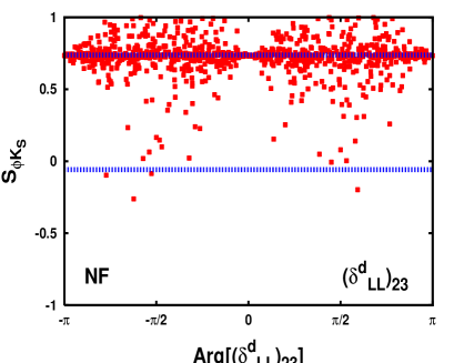
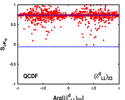
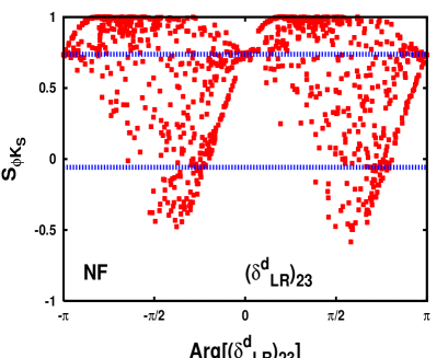
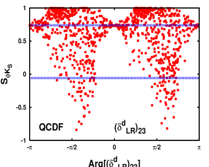
Figure 5: $S_{\Phi K_{S}}$ as a function of arg[${\left(\delta^{d}_{LL}\right)_{23}}$] (top) and arg[${\left(\delta^{d}_{LR}\right)_{23}}$] (bottom) with gluino contribution of one mass insertion ${\left(\delta^{d}_{LL}\right)_{23}}$ (top) and ${\left(\delta^{d}_{LR}\right)_{23}}$ (down). Left and right plots correspond to NF and QCDF, respectively. The region inside the two horizontal lines corresponds to the allowed experimental region at $2\sigma$ level.

We present our numerical results for the gluino contributions to CP asymmetry $S_{\Phi K_{S}}$ in Figs. 5. The left and right plots correspond to the evaluation of amplitudes by means of NF and QCDF methods, respectively. In all the plots, regions inside the horizontal lines indicate the allowed $2\sigma$ experimental range. In the top and bottom plots only one mass insertion per time is taken active, in particular this means that we scanned over $|{\left(\delta^{d}_{LL}\right)_{23}}|<1$ and $|{\left(\delta^{d}_{LR}\right)_{23}}|<1$. Then, $S_{\Phi K_{S}}$ is plotted versus $\theta_{\phi}$, which in the case of one dominant mass insertion should be identified here as $\theta_{\phi}={\rm arg}[(\delta_{AB}^{d})_{ij}]$.

We have scanned over the relevant SUSY parameter space, in this case the average squark mass $\tilde{m}$ and gluino mass $m_{\tilde{g}}$, assuming SM central values [55]. Moreover, we require that the SUSY spectra satisfy the present experimental lower mass bounds [55]. In particular, $m_{\tilde{g}}>200$ GeV, $\tilde{m}>300$ GeV. In addition, we impose that the branching ratio (BR) of $b\to s\gamma~{}$and the $B-\bar{B}~{}$mixing are satisfied at 95% C.L. [59], namely $2\times 10^{-4}\leq BR(b\to s\gamma)<4.5\times 10^{-4}$. Then, the allowed ranges for $|{\left(\delta^{d}_{LL}\right)_{23}}|$ and $|{\left(\delta^{d}_{LR}\right)_{23}}|$ are obtained by taken into account the above constraints on $b\to s\gamma~{}$and $B-\bar{B}~{}$mixing.

In the plots corresponding to QCDF, we have also scanned over the full range of the parameters $\rho_{A,H}$ and $\phi_{A,H}$ in $X_{A}$ and $X_{H}$, respectively, as defined in Eq.(29). We remind here that $X_{A}$ and $X_{H}$ take into account the (unknown) infrared contributions in the hard scattering and annihilation diagrams. Regarding the allowed range of $\rho$, as can be seen from results in Eq.(33), the dominant effect is due to the annihilation contributions proportional to $X_{A}$. As discussed in section 3, the total width will grow as $\rho_{A}^{4}\log^{4}{\left(m_{b}/\Lambda\right)}$ for large $\rho_{A}$ . Therefore, as we will show in section 5, by requiring that the SUSY contribution to the branching ratio and asymmetries of $B\to\phi K_{S}$ is inside the $2\sigma$ experimental range, an upper bound on $\rho_{A}$ of order $\rho_{A}\simeq 2$ is obtained.

In the corresponding plots evaluated in NF, in order to maximize the SUSY contributions to CP asymmetry, we have fixed the average of gluon momenta to its minimum value $\langle q^{2}\rangle=m_{b}^{2}/4$. We remind here that $\langle q^{2}\rangle$ enters as free parameter in matrix element of the chromo-magnetic operator $Q_{8g}$, see Eq.(23). As we will show later on, the dominant SUSY effect to $B\to\phi K_{S}$ amplitude is given by the SUSY contribution to the Wilson coefficient $C_{8g}$. Therefore, the smaller the $\langle q^{2}\rangle$ value is, the larger the SUSY contribution to the CP asymmetry can be.

In the framework of NF, the strong phase, which comes from the hadronic matrix elements, cannot be predicted. For this reason we set both SM and SUSY strong phases to zero. Therefore, the phase $\delta_{\phi}$ in Eq.(44) can take only the values $0$ or $\pi$, corresponding to the relative sign of SM and SUSY amplitudes.

By comparing the scatter plots in NF and QCDF in Fig. 5 we see that the predictions are quite similar. Only the gluino contributions proportional to ${\left(\delta^{d}_{LR}\right)_{23}}$ have chances to drive $S_{\Phi K_{S}}$ toward the region of large and negative values, while the pure effect of ${\left(\delta^{d}_{LL}\right)_{23}}$ just approach the negative values region.

This result can be easily understood by noticing that the dominant SUSY source to the $B\to\phi K_{S}$ decay amplitude is provided by the chromo-magnetic operator $Q_{8g}$. In particular, as already mentioned in section 2, gluino contributions to $C_{8g}$, which are proportional to ${\left(\delta^{d}_{LR}\right)_{23}}$, can be very large with respect to the SM ones, being enhanced by terms of order $m_{\tilde{g}}/m_{b}$. In addition, large gluino effects in $C_{8g}$ may still escape $b\to s\gamma~{}$constraints [58]. This is a remarkable property and it is due to the fact that in the gluino contributions to dipole operators $Q_{7\gamma,8g}$, the ratio of $|C_{8g}/C_{7\gamma}|$ is enhanced by color factors with respect to typical contributions of W or chargino exchanges [48].

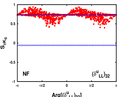
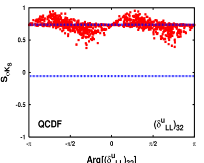
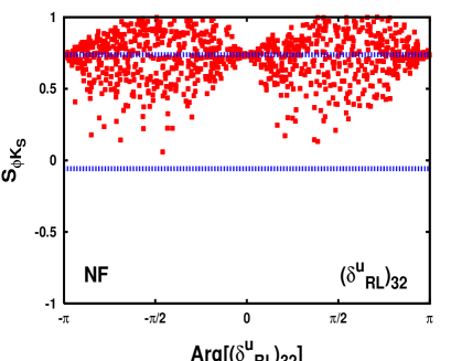
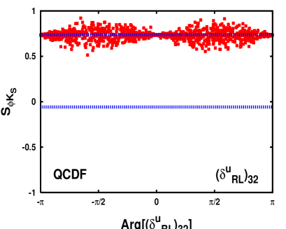
Figure 6: As in Fig. 5, but for $S_{\Phi K_{S}}$ as a function of arg[${\left(\delta^{u}_{LL}\right)_{32}}$] (top) and arg[${\left(\delta^{u}_{RL}\right)_{32}}$] (bottom) with chargino contribution of one mass insertion ${\left(\delta^{u}_{LL}\right)_{32}}$ (top) and ${\left(\delta^{u}_{RL}\right)_{32}}$ (down).

Now we discuss the chargino effects to $S_{\phi K_{S}}$, which are summarized in Fig. 6. These contributions have been first analyzed, in the framework of MIA, in Ref.[11], but only using NF approach for evaluating the hadronic matrix elements. Here, we extend our previous analysis in [11] by including the corresponding predictions in the QCDF approach. In Fig. 6, $S_{\phi K_{S}}$ is plotted versus the argument of the relevant chargino mass insertions, namely ${\left(\delta^{u}_{LL}\right)_{32}}$ and ${\left(\delta^{u}_{RL}\right)_{32}}$. Same conventions as in Fig. 5 have been adopted for left and right plots.

As in the gluino dominated scenario, we have scanned over the relevant SUSY parameter space, in particular, the average squark mass $\tilde{m}$, weak gaugino mass $M_{2}$, the $\mu$ term, and the light right stop mass $\tilde{m}_{\tilde{t}_{R}}$. Also $\tan{\beta}=40$ has been assumed and we take into account the present experimental bounds on SUSY spectra, in particular $\tilde{m}>300$ GeV, the lightest chargino mass $M_{\chi}>90$ GeV, and $\tilde{m}_{\tilde{t}_{R}}\geq 150$ GeV. As in the gluino case, we scan over the real and imaginary part of the mass insertions ${\left(\delta^{u}_{LL}\right)_{32}}$ and ${\left(\delta^{u}_{RL}\right)_{32}}$, by considering the constraints on BR($b\to s\gamma~{}$) and $B-\bar{B}~{}$mixing at 95% C.L.. The $b\to s\gamma~{}$constraints impose stringent bounds on ${\left(\delta^{u}_{LL}\right)_{32}}$, specially at large $\tan{\beta}$ [11]. Finally, as in the other plots, we scanned over the QCDF free parameters $\rho_{A,H}<2$ and $0<\phi_{A,H}<2\pi$.

From these results we can see that also for the chargino dominated scenario the predictions in NF and in QCDF are quite close, apart from a slight difference in the ${\left(\delta^{u}_{RL}\right)_{32}}$ ones that we will discuss below. The main conclusion in this scenario is that negative values of $S_{\phi K_{S}}$ cannot be achieved neither in NF nor in QCDF.

The reason why extensive regions of negative values of $S_{\phi K_{S}}$ are excluded here, is only due to the $b\to s\gamma~{}$constraints [11]. Indeed, as shown in our previous work [11], the inclusion of ${\left(\delta^{u}_{LL}\right)_{32}}$ mass insertion can generate large and negative values of $S_{\phi K_{S}}$, by means of chargino contributions to chromo-magnetic operator $Q_{8g}$ which are enhanced by terms of order $m_{\chi^{\pm}}/m_{b}$. However, contrary to the gluino scenario, the ratio $|C_{8g}/C_{7\gamma}|$ is not enhanced by color factors and large contributions to $C_{8g}$ leave unavoidably to the breaking of $b\to s\gamma~{}$constraints.

On the other hand, the contribution of ${\left(\delta^{u}_{RL}\right)_{32}}$ is independent of $\tan{\beta}$ and so large effects in $R_{\phi}$ that could drive $S_{\phi K_{S}}$ toward the region of negative values cannot be achieved. However, as can be seen from Fig. 6, while both in NF ${\left(\delta^{u}_{RL}\right)_{32}}$ and ${\left(\delta^{u}_{LL}\right)_{32}}$ contributions are within the 2$\sigma$ experimental range, in NF the ${\left(\delta^{u}_{RL}\right)_{32}}$ contribution fits better than in QCDF. This can be explained by the fact that ${\left(\delta^{u}_{RL}\right)_{32}}$ mainly gives contribution to the electroweak operators, whose matrix elements are more sensitive, with respect to the other operators, to the approach adopted for their evaluation.

As shown in our previous work [11], by scanning over the two relevant mass insertions ${\left(\delta^{u}_{RL}\right)_{32}}$ and ${\left(\delta^{u}_{LL}\right)_{32}}$, the $b\to s\gamma~{}$constraints on ${\left(\delta^{u}_{LL}\right)_{32}}$ are a bit more relaxed, but a large amount of fine tuning between SUSY parameters is necessary if small values of $S_{\phi K_{S}}$ are required.

In order to understand the behavior of these results, it is useful to look at the numerical parametrization of the ratio of amplitudes ${\cal R}_{\phi}\equiv\frac{A_{SUSY}(B\to\phi K_{S})}{A_{SM}(B\to\phi K_{S})}$ in terms of the relevant mass insertions. Below, we present numerical results for ${\cal R}_{\phi}$ in both NF and QCDF. In QCDF we set to zero the effect of annihilation and hard scattering diagrams, corresponding to the choice of $\rho_{A,H}=0$ and $\phi_{A,H}=\pi$. In this case, we expect QCDF predictions to be quite close to the NF ones. In particular, for a gluino mass and average squark mass of order $\tilde{m}=m_{\tilde{g}}=500$ GeV, we obtain

$${\cal R}_{\phi}|^{NF}_{\tilde{g}} \simeq \left\{-0.08\,{\left(\delta^{d}_{LL}\right)_{23}}\,-\,120\,{\left(\delta^{d}_{LR}\right)_{23}}\right\}\,+\,\left\{L\leftrightarrow R\right\},$$

$${\cal R}_{\phi}|^{QCDF}_{\tilde{g}} \simeq \left\{-0.14\,\times e^{-i\,0.1}{\left(\delta^{d}_{LL}\right)_{23}}\,-\,127\,\times e^{-i\,0.08}{\left(\delta^{d}_{LR}\right)_{23}}\right\}\,+\,\left\{L\leftrightarrow R\right\},$$ (55)

while in the case of chargino, by using gaugino mass $M_{2}=200$ GeV, $\mu=300$ GeV, $\tilde{m}_{\tilde{t}_{R}}=150$ GeV, and $\tan{\beta}=40$, we have

$${\cal R}_{\phi}|^{NF}_{\chi} \simeq 1.83\,{\left(\delta^{u}_{LL}\right)_{32}}\,-\,0.32\,{\left(\delta^{u}_{RL}\right)_{32}}\,+\,0.41\,{\left(\delta^{u}_{LL}\right)_{31}}\,-\,0.07\,{\left(\delta^{u}_{RL}\right)_{31}},$$

$${\cal R}_{\phi}|^{QCDF}_{\chi} \simeq 1.89\times e^{-i\,0.07}\,{\left(\delta^{u}_{LL}\right)_{32}}\,-\,0.11\times e^{-i\,0.17}\,{\left(\delta^{u}_{RL}\right)_{32}}$$ (56)

$$+ 0.43\times e^{-i\,0.07}\,{\left(\delta^{u}_{LL}\right)_{31}}\,-\,0.02\times e^{-i\,0.17}\,{\left(\delta^{u}_{RL}\right)_{31}}.$$

where the first symbol ${\cal R}_{\phi}|_{\tilde{g}}^{NF}$ means that the corresponding quantity ${\cal R}_{\phi}$ has been calculated in NF approach including only gluino contributions. Analogously for the other cases of QCDF and for chargino ($\chi$) exchanges.

From results in Eqs.(55)–(56), it is clear that the largest SUSY effect is provided by the gluino and chargino contributions to the chromo-magnetic operator which are proportional to ${\left(\delta^{d}_{LR}\right)_{23}}$ and ${\left(\delta^{u}_{LL}\right)_{32}}$, respectively. However, the $b\to s\gamma~{}$constraints play a crucial role in this case. For the above SUSY configurations, the $b\to s\gamma~{}$decay set the following (conservative) constraints on gluino and chargino contributions: $|{\left(\delta^{d}_{LR}\right)_{23}}|<0.019$ and $|{\left(\delta^{u}_{LL}\right)_{32}}|<0.20$. Implementing these bounds in Eqs.(55)–(56), we see that gluino contribution can easily achieve larger values of $R_{\phi}=|{\cal R}_{\phi}|$ (see Eqs.(LABEL:ratioPHI),(51)) than chargino one, and this is the main reason why extensive regions with negative value of $S_{\phi K_{S}}$ are favored and disfavored in Figs. 5 and 6, respectively.

4.2 CP asymmetry in $B\to{\eta^{\prime}K_{S}}$ decay

Recent measurements of CP asymmetry in $B\to{\eta^{\prime}K_{S}}$ show another discrepancy with SM predictions. In particular from Eq.(4), the world average is

$$S_{\eta^{\prime}K_{S}} = 0.41\pm 0.11\,,$$ (57)

and which is about $2.5\sigma$ deviation from SM expectations. From these results we see that, similarly to what happens in $B\to\phi K_{S}$ decay, large deviations from SM are possible.

Since SUSY contributes to both CP asymmetries with the same CP violating source, it is possible that the SUSY effects driving $S_{\phi K_{S}}$ towards negative values, could also sizeably decrease $S_{\eta^{\prime}K_{S}}$. The main reason for that is because the leading SUSY contributions to the amplitudes of $B\to\phi K_{S}$ and $B\to\eta^{\prime}K_{S}$ enter through the Wilson coefficient of $C_{8g}$ and the operator $Q_{8g}$ has a comparable matrix elements in both processes. However, since NP corrections enter through the quantity $R_{\eta^{\prime}}$, the role of the SM contribution will be crucial. Indeed, while the $B\to\phi K_{S}$ amplitude is purely generated at one-loop in the SM, the $B\to\eta^{\prime}K_{S}$ one receives tree-level contribution from the SM by means of non-vanishing matrix element of $Q_{2}$. Therefore, the increase of SUSY contributions to $C_{8g}$ is now compensated in $R_{\eta^{\prime}}$, by the large SM amplitude contribution.

We show our results for gluino in Fig. 7, where we have just extended the same analysis of $B\to\phi K_{S}$. Same conventions as in figures for $B\to\phi K_{S}$ have been adopted here. As we can see from these results, there is a depletion of the gluino contribution in $S_{\eta^{\prime}K_{S}}$, precisely for the reasons explained above. Regions of negative values of $S_{\eta^{\prime}K_{S}}$ are more disfavored with respect to $S_{\phi K_{S}}$, but a minimum of $S_{\eta^{\prime}K_{S}}\simeq 0$ can be easily achieved. Comparing NF and QCDF, we can also see that SUSY predictions in NF and QCDF are very close.

Finally, in Fig. 8 we present our results for chargino contributions. Here we see that charginos can produce at most a deviation from SM predictions of about $\pm 20$ %, and the most conspicuous effect is achieved by ${\left(\delta^{u}_{LL}\right)_{32}}$. These results again show the relevant role played by the chromo-magnetic operator.

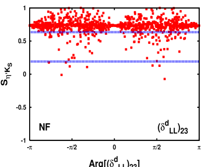
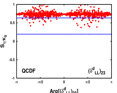
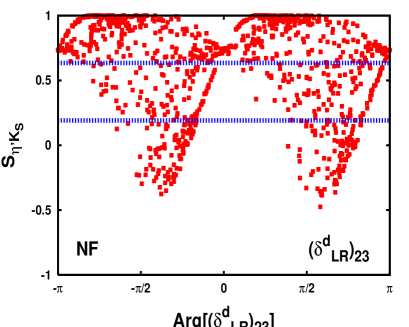
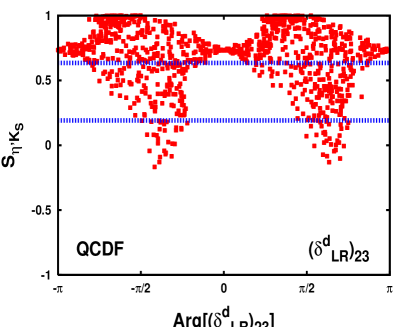
Figure 7: As in Fig. 5, but for $S_{\eta^{\prime}K_{S}}$.

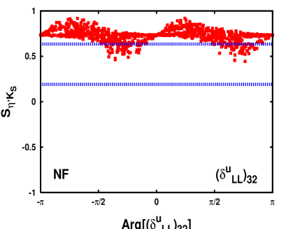
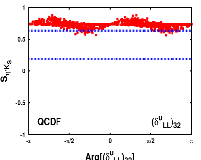
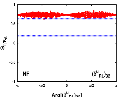
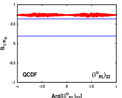
Figure 8: As in Fig. 6, but for $S_{\eta^{\prime}K_{S}}$.

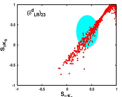
Figure 9: Correlation of asymmetries $S_{\Phi K_{S}}$ versus $S_{\eta^{\prime}K_{S}}$ with the contribution of one mass insertion ${\left(\delta^{u}_{RL}\right)_{32}}$ (left) and ${\left(\delta^{d}_{LR}\right)_{23}}$ (right), for chargino (left) and gluino (right) exchanges. Region inside the ellipse corresponds to the allowed experimental ranges at $2\sigma$ level.

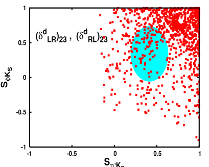
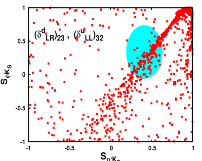
Figure 10: As in Fig. 9, but for arg[${\left(\delta^{d}_{LR}\right)_{23}}$]=arg[${\left(\delta^{d}_{RL}\right)_{23}}$] (left) and arg[${\left(\delta^{d}_{LR}\right)_{23}}$]=arg[${\left(\delta^{u}_{LL}\right)_{32}}$] (right), with the contribution of two mass insertions ${\left(\delta^{d}_{LR}\right)_{23}}$ & ${\left(\delta^{d}_{RL}\right)_{23}}$ (left) for gluino exchanges, and ${\left(\delta^{d}_{LR}\right)_{23}}$ & ${\left(\delta^{u}_{LL}\right)_{32}}$ (right) for both gluino and chargino exchanges.

As in the case of $B\to\phi K_{S}$ decay, we present below the parametrization of ${\cal R}_{\eta^{\prime}}\equiv\frac{A_{SUSY}(B\to\eta^{\prime}K_{S})}{A_{SM}(B\to\eta^{\prime}K_{S})}$, by using the same SUSY inputs adopted in Eqs. (56), (55). For gluino contributions we have

$${\cal R}_{\eta^{\prime}}|^{NF}_{\tilde{g}} \simeq \left\{-0.08\,{\left(\delta^{d}_{LL}\right)_{23}}\,-\,79\,{\left(\delta^{d}_{LR}\right)_{23}}\right\}\,-\,\left\{L\leftrightarrow R\right\},$$

$${\cal R}_{\eta^{\prime}}|^{QCDF}_{\tilde{g}} \simeq \left\{-0.07\,\times e^{i\,0.24}{\left(\delta^{d}_{LL}\right)_{23}}\,-\,64{\left(\delta^{d}_{LR}\right)_{23}}\right\}\,-\,\left\{L\leftrightarrow R\right\},$$ (58)

while for chargino exchanges we obtain

$${\cal R}_{\eta^{\prime}}|^{NF}_{\chi} \simeq 1.2\,{\left(\delta^{u}_{LL}\right)_{32}}\,-\,0.01\,{\left(\delta^{u}_{RL}\right)_{32}}\,+\,0.27\,{\left(\delta^{u}_{LL}\right)_{31}}\,-\,0.002\,{\left(\delta^{u}_{RL}\right)_{31}},$$

$${\cal R}_{\eta^{\prime}}|^{QCDF}_{\chi} \simeq 0.95\,{\left(\delta^{u}_{LL}\right)_{32}}\,-\,0.025\times e^{-i\,0.19}\,{\left(\delta^{u}_{RL}\right)_{32}}$$ (59)

$$+ 0.21\,{\left(\delta^{u}_{LL}\right)_{31}}\,-\,0.006\times e^{-i\,0.19}\,{\left(\delta^{u}_{RL}\right)_{31}}\,.$$

Notice that in the second curly brackets in Eq.(58) there is a minus sign in front. This takes into account for the minus sign in the matrix elements of $\tilde{Q}_{i}$ operators as shown in Eq.(42).

In both cases of gluino and chargino contributions, we see that the coefficient of ${\left(\delta^{d}_{LR}\right)_{23}}$ and ${\left(\delta^{u}_{LL}\right)_{32}}$ mass insertions is smaller in comparison than the corresponding ones in $B\to\phi K_{S}$, see Eqs.(55), (56). As explained before, this depletion comes from the fact that the SM amplitude of $A(B\to\eta^{\prime}K_{S})$ receives contribution from tree-level $W$ exchanges and it is larger than $A(B\to\phi K_{S})$.

This general behavior is going in the right direction to explain the experimental data. In order to show better this effect, we plotted in Figs. 9 the correlations between $S_{\phi K_{S}}$ versus $S_{\eta^{\prime}K_{S}}$ for both chargino (left plot) and gluino (right plot) in QCDF. For illustrative purposes, in all figures analyzing correlations, we colored the area of the ellipse corresponding to the allowed experimental range at $2\sigma$ level. In Fig. 9 we scanned over the real and imaginary part of the single relevant mass insertions, namely ${\left(\delta^{u}_{RL}\right)_{32}}$ (left plot) and ${\left(\delta^{d}_{LR}\right)_{23}}$ (right plot) for chargino and gluino, respectively.

In conclusion, as can be seen from the results in Fig. 9, pure chargino exchanges have no chance to fit data at $2\sigma$ level, while gluino can fit them quite well. At this point we want to stress that sizeable chargino contributions to the CP asymmetries, in particular from ${\left(\delta^{u}_{LL}\right)_{32}}$ mass insertion, are ruled out by $b\to s\gamma$ constraints. Therefore, it would be interesting to see if the effects of a light charged Higgs exchange could relax these constraints allowing chargino contributions to fit inside the experimental ranges.

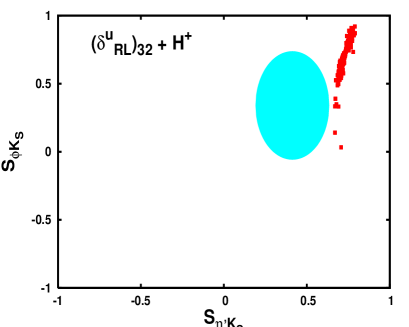
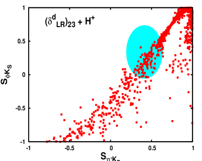
Figure 11: As in Fig. 9, but taking into account a charged Higgs exchange with mass $m_{H}=200$ GeV and $\tan{\beta}=40$.

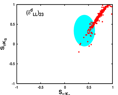
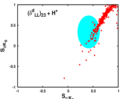
Figure 12: As in Fig. 9, but for gluino contributions with single mass insertion ${\left(\delta^{d}_{LL}\right)_{23}}$. In the right plot the effect of a charged Higgs exchange, with mass $m_{H}=200$ GeV and $\tan{\beta}=40$, has been taken into account.

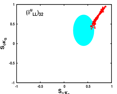
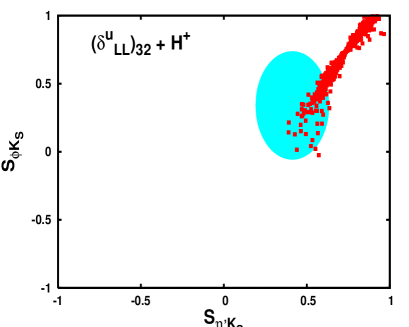
Figure 13: As in Fig. 12, but for chargino contribution with single mass insertion ${\left(\delta^{u}_{LL}\right)_{32}}$.

For this purpose, we present in Figs. 11-13 the impact of a light charged Higgs in both chargino and gluino exchanges. In particular, plots in Fig. 9 should be directly compared with the corresponding ones in Fig. 11, where a charged Higgs with mass $m_{H}=200$ GeV and $\tan{\beta}=40$ has been taken into account. From these results we can see that the effects of charged Higgs exchange in the case of ${\left(\delta^{u}_{RL}\right)_{32}}$ mass insertion are negligible, as we expect from the fact that terms proportional to ${\left(\delta^{u}_{RL}\right)_{32}}$ in $b\to s\gamma$ and $b\to sg$ amplitudes are not enhanced by $\tan{\beta}$. On the other hand, in gluino exchanges with ${\left(\delta^{d}_{LR}\right)_{23}}$ or ${\left(\delta^{d}_{LL}\right)_{23}}$ (see Figs. 11,12), the most conspicuous effect of charged Higgs contribution is in populating the area outside the allowed experimental region. This is clearly due to a destructive interference with $b\to s\gamma$ amplitude, which relaxes the $b\to s\gamma$ constraints. The most relevant effect of a charged Higgs exchange is in the scenario of chargino exchanges with ${\left(\delta^{u}_{LL}\right)_{32}}$ mass insertion. In this case, as can be seen from Fig. 13, a strong destructive interference with $b\to s\gamma$ amplitude can relax the $b\to s\gamma$ constraints in the right direction, allowing chargino predictions to fit inside the experimental region. Moreover, we have checked that, for $\tan{\beta}=40$, charged Higgs heavier than approximately 600 GeV cannot affect the CP asymmetries significantly.

In a recent paper [9], it has been shown that there exists a particular scenario in which gluino contribution can sizeably decrease $S_{\phi K_{S}}$ providing on the same time a very modest effect in $S_{\eta^{\prime}K_{S}}$. This can be achieved if one assume that both ${\left(\delta^{d}_{LR}\right)_{23}}$ and ${\left(\delta^{d}_{RL}\right)_{23}}$ mass insertions are of the same order, including their CP violating phase. In this case gluino contributes with the same weight to both $Q_{i}$ and $\tilde{Q}_{i}$ operators in Eq.(7), where $\tilde{Q}_{i}$ are the operators with opposite chirality. Due to the different parity of the final states, as explained in section 3, the contribution of the corresponding Wilson coefficients to the amplitude of $B\to\phi K_{S}$ and $B\to\eta^{\prime}K_{S}$ enter in combination as $C_{i}+\tilde{C}_{i}$ and $C_{i}-\tilde{C}_{i}$, respectively.

However, the analysis of Ref. [9] was based on the NF approach, and one may wonder, if their results still hold in QCDF. For this reason we repeat here the same analysis, but in QCDF and scanning over the strong CP phases $\phi_{A,H}$ and $\rho_{A,H}<2$. Results of this scenario are shown in Fig. 10 (left plot), where we scanned over two mass insertions simultaneously, namely ${\left(\delta^{d}_{LR}\right)_{23}}$ and ${\left(\delta^{d}_{RL}\right)_{23}}$, by assuming that their CP violating phases are the same. From these results we can see that a large number of SUSY configuration fitting inside the $2\sigma$ experimental region, can be obtained.

We have also considered another scenario in which both chargino and gluino exchanges are assumed to contribute simultaneously with relevant mass insertions, namely ${\left(\delta^{d}_{LR}\right)_{23}}$ and ${\left(\delta^{u}_{LL}\right)_{32}}$. We plot the corresponding results for the correlations between $S_{\phi K_{S}}$ versus $S_{\eta^{\prime}K_{S}}$ in the right plot of Fig. 10. As in the case of Fig. 9, we assume a common SUSY CP violating phase between the two mass insertions. From these results we can see that also in this case a large number of configurations can fit inside the $2\sigma$ experimental regions. This result shows a remarkable fact. The stringent bounds on ${\left(\delta^{u}_{LL}\right)_{32}}$ from the experimental limits on $BR(B\to X_{s}\gamma)$ are relaxed when one considers both gluino and chargino contributions, which come with different sign. This does not happen, if two chargino mass insertions are considered. Then some configurations with large $\tan\beta$ are allowed and therefore chargino can contribute significantly to the CP asymmetries $S_{\phi K_{S}}$ and $S_{\eta^{\prime}K_{S}}$.

Finally, we would like to comment about the stability of SUSY predictions for $S_{\phi K_{S}}$ against the low renormalization scale $\mu_{b}$, where Wilson coefficients are evaluated. In NF the scale dependence in the Wilson coefficients is not compensated by the corresponding one in the matrix elements, so a large uncertainty is expected. However, we have noticed that also in QCDF this uncertainty still persists. In particular the coefficients in the parametrizations in QCDF in Eq. (55)–(56) can vary up to 30-40 % when the $\mu_{b}$ scale is changed from $\mu_{b}=m_{b}/2$ to $\mu_{b}=m_{b}$. All the numerical results in this paper correspond to the choice $\mu_{b}=m_{b}^{\rm pole}=4.5$ GeV. In both NF and QCDF, this residual scale dependence in $R_{\phi}$ is mainly due to the scale dependence in the SM amplitude and in the $C_{8g}(\mu_{b})$ contribution to the SUSY amplitude. However, we noticed that the main sensitivity to the scale in $R_{\phi}$ comes from the SM contribution. On the other hand, the main source of sensitivity in $R_{\eta^{\prime}}$ comes from $C_{8g}(\mu_{b})$ in the SUSY amplitude, since the SM one, receiving tree-level contributions, is less sensitive to the renormalization scale.

In the next section we are going to consider the correlations of $S_{\phi K_{S}}$ and $S_{\eta^{\prime}K_{S}}$ asymmetries versus the corresponding branching ratios of $B\to\phi K_{S}$ and $B\to\eta^{\prime}K_{S}$.

5 SUSY contributions to $BR(B\to\phi(\eta^{\prime})K)$

In this section we discuss the impact of large SUSY contribution, which is required to explain the deviations from SM in CP asymmetries of $S_{\phi(\eta^{\prime})K_{S}}$, on the branching ratios (BR) of $B\to\phi K$ and $B\to\eta^{\prime}K$. As shown in Eqs.(5),(6), the experimental measurements of these BRs at BaBar, Belle, and CLEO lead to the following averaged results [25]:

$$BR(B\to\phi K) = (8.3^{+1.2}_{-1.0})\times 10^{-6},$$ (60)

$$BR(B\to\eta^{\prime}K) = (65.2^{+6.0}_{-5.9})\times 10^{-6}.$$ (61)

which mean that $BR(B\to\phi K)$ is in good agreement with SM predictions, while the experimental value of $BR(B\to\eta^{\prime}K)$ is two to five times larger than the SM one. Since these two processes are highly correlated and both are based on the $b\to s$ transition, it seems a challenge for the SUSY contribution to enhance $BR(B\to\eta^{\prime}K)$ by a factor of two or more, while leaving other BRs and asymmetries inside their experimental ranges.

The branching ratio of $B\to MK$, with $M=\phi$ or $\eta^{\prime}$, can be written in terms of the corresponding amplitude ${\cal M}_{M}$ as

$$BR(B\to MK)=\frac{1}{8\pi}\frac{|P|}{M_{B}^{2}}|\mathcal{M}_{M}|^{2}\frac{1}{\Gamma_{tot}},$$ (62)

where $\mathcal{M}_{M}=\langle M\bar{K}^{0}|H_{eff}^{\Delta B=1}|\bar{B}^{0}\rangle$ and

$$|P|=\frac{\left[\left(M_{B}^{2}-(m_{K}+m_{M})^{2}\right)\left(M_{B}^{2}-(m_{K}-m_{M})^{2}\right)\right]^{1/2}}{2M_{B}}.$$ (63)

The inclusion of SUSY corrections modifies the BR as

$$BR^{\mbox{\tiny total}}(B\to MK)=BR^{\mbox{\tiny SM}}(B\to MK)\times\left[1+2\cos(\theta_{M}-\delta_{M})R_{M}+R_{M}^{2}\right]$$ (64)

where $R_{M}=\left|\frac{A^{\mathrm{SUSY}}(B\to MK)}{A^{\mathrm{SM}}(B\to MK)}\right|$, $\theta_{M}=arg\left[\frac{A^{\mathrm{SUSY}}(B\to MK)}{A^{\mathrm{SM}}(B\to MK)}\right]$ and $\delta_{M}$ is the corresponding strong phase. The input parameters that we have used in the previous section with $\rho_{A,H}=1$ and $\phi_{A,H}=\pi$ i.e. $X_{A,H}=0$ lead to $BR^{\mbox{\tiny SM}}(B\to\phi K)=2.76\times 10^{-6}$ and $BR^{\mbox{\tiny SM}}(B\to\eta^{\prime}K)=11.1\times 10^{-6}$.

It is remarkable that in order to produce the experimental result of $S_{\phi K_{S}}$ by SUSY contribution, the phase $\theta_{\phi}=arg\left[\frac{A^{\mathrm{SUSY}}(B\to\phi K_{S})}{A^{\mathrm{SM}}(B\to\phi K_{S})}\right]$ has to be around $\pm\pi/2$ and the strong phase $\delta_{\phi}$ should be of order $\pi$ or $0$, as shown in section 4. These particular values for the phases suppress the leading term in Eq. (64). Therefore, for typical scenarios in which $R_{\phi}\leq 1$, the SUSY contributions do not enhance $BR(B\to\phi K)$ much. At most a total branching ratio of order $3\times BR^{\mbox{\tiny SM}}(B\to\phi K)\simeq 8.3\times 10^{-6}$ can be achieved, as we will explain below, which is still compatible with the experimental measurements. Clearly, if $R_{\phi}\gg 1$ then the total branching ratio would exceed the experimental bound in Eq.(60). However, as shown in section 3, the inclusion of $b\to s\gamma$ constraints moderates possible large SUSY contributions to $R_{\phi}$.

Next we briefly discuss the dependence of the branching ratio on the QCDF free parameters $\rho_{A,H}$, related to annihilation and hard scattering diagrams. The only relevant parameter here is the $\rho_{A}$ one, while regarding $\rho_{H}$, the BR shows a moderate dependence [44]. By using dimensional analysis, one can see that for large values of $\rho_{A}$, $BR^{\mbox{\tiny SM}}(B\to\phi K)$ scales like $\rho_{A}^{4}$. This result suggests that one can set very strong upper bounds on $\rho_{A}$ by requiring that $BR^{\mbox{\tiny SM}}(B\to\phi K)$ does not exceed experimental range. Clearly, when new corrections beyond the SM ones are included, upper bounds on $\rho_{A}$ could be relaxed due to possible negative interferences between SM and new physics amplitudes.

In order to understand the impact of the annihilation diagrams on $BR(B\to\phi K)$, we show below the explicit dependence of the SM amplitude on the parameters $\rho_{A}$ and $\phi_{A}$:

$$i\,A^{SM}(B\to\phi K_{S})\simeq-1.8\times 10^{-8}+7.9\times 10^{-10}X_{A}-6.1\times 10^{-10}X_{A}^{2}+2.2\times 10^{-10}X_{H}$$ (65)

where numbers in the right hand side of Eq.(65) are in unity of GeV, and $X_{A,H}$ are defined in Eqs.(29). We have used SM central values as in Table 1 of [44], and omitted contributions from imaginary parts which are quite small.

As can be seen from Eqs.(65) and (29), for $\rho_{A}\gg 1$ the SM amplitude could be doubled and hence the SM branching ratio would be about four times the result with $\rho_{A}<1$, therefore exceeding the present experimental range. As shown in Ref.[44], and in Fig. 14 (see lighter dashed line), the constraint on $\rho_{A}$ is already obtained for moderate values of $\rho_{A}\raise 1.29167pt\hbox{$\;<$\kern-7.5pt\raise-4.73611pt\hbox{$\sim\;$}}2$.

It would be interesting to see how much the upper bounds on $\rho_{A}$ could be modified by the inclusion of SUSY corrections, while satisfying all the experimental constraints.

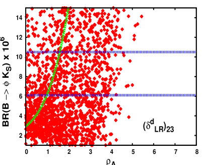
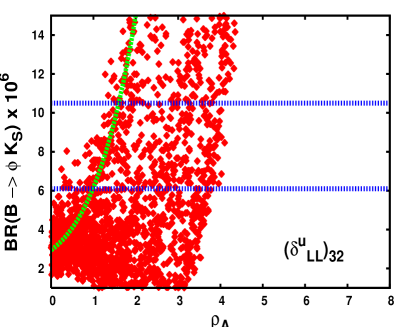
Figure 14: $BR(B\to\phi K)$ as function of the annihilation parameter $\rho_{A}$ and for $\rho_{H}=1$, $\phi_{A,H}=0$, for one mass insertion contribution of gluino ${\left(\delta^{d}_{RL}\right)_{23}}$ (left) and chargino ${\left(\delta^{u}_{LL}\right)_{32}}$ (right). Lighter dashed line corresponds to the SM case. The region inside the two horizontal lines corresponds to the allowed experimental range at $2\sigma$ level.

For this purpose, we plot in Fig. 14 the total branching ratio of $B\to K\phi$ as a function of $\rho_{A}$ for gluino and chargino contribution. We present the gluino results for the case of LR dominant scenario, and the chargino ones with the LL dominant case. The values of these mass insertions are varied in the allowed range as done for the other plots. Also we scanned over the different values of the strong phases $\phi_{A,H}$, squark masses, gluino and chargino masses. In these plots, the dashed lines correspond to the SM predictions for $BR(B\to K\phi)$. As can be seen from this figure, by applying the $2\sigma$ constraints on $BR^{SM}(B\to K\phi)$ one can set very stringent upper bounds on $\rho_{A}$, namely $\rho\raise 1.29167pt\hbox{$\;<$\kern-7.5pt\raise-4.73611pt\hbox{$\sim\;$}}2$. On the other hand, this bound can be relaxed to $\rho\raise 1.29167pt\hbox{$\;<$\kern-7.5pt\raise-4.73611pt\hbox{$\sim\;$}}4$ and $\rho\raise 1.29167pt\hbox{$\;<$\kern-7.5pt\raise-4.73611pt\hbox{$\sim\;$}}5$, in the case of LL and LR mass insertion contributions in up- and down-squark, respectively. However, it is important to note that most of the configurations in both gluino and chargino cases that allow for $\rho>2$ lead to CP asymmetry $S_{\phi K_{S}}$ outside the $2\sigma$ range of the experimental results. Therefore, as mentioned above, we consider $\rho<2$ as a conservative bound.

Regarding the $BR(B\to\eta^{\prime}K)$, we find that it is less sensitive to $\rho_{A}$ than $BR(B\to\phi K)$. This can be easily observed from the dependence of the amplitude of $B\to\eta^{\prime}K$ on $X_{A}$. Analogously to Eq.(65), we get

$$i\,A^{SM}(B\to\eta^{\prime}K)\simeq 3.6\times 10^{-8}+0.19\times 10^{-10}X_{A}+4.2\times 10^{-10}X_{A}^{2}+7.7\times 10^{-10}X_{H}\,,$$ (66)

where, as in Eq.(65), numbers in the r.h.s. of Eq.(66) are expressed in units of GeV. Thus, comparing Eqs.(65) and (66), we see that the effect of $\rho_{A}$ in $A_{SM}(B\to\eta^{\prime}K)$ is suppressed by two orders of magnitude with respect to the same one in $A_{SM}(B\to\phi K)$. Hence the strongest bound one can obtain on $\rho_{A}$ will come only from $BR(B\to\phi K)$. Therefore, in all plots of the present work, including the QCDF ones in section 4, we scanned over $\rho_{A}$ by requiring $\rho_{A}\leq 2$.

As mentioned before, the experimental measurements of $BR(B\to\eta^{\prime}K)$ represent another large discrepancy with the SM prediction. There have been various efforts to explain the large observed branching ratio in the $B\to\eta^{\prime}K$ process, based on the peculiarity of $\eta^{\prime}$ meson. For instance, intrinsic charm [31] or gluonium contents of $\eta^{\prime}$ [32], have been investigated as possible new sources for such an enhancement. Clearly, NP contributions could also be responsible of such discrepancy in $BR(B\to\eta^{\prime}K_{s})$, or at least for a part of it. In this respect, we are going to analyze next the maximum effect that one can obtain from SUSY contributions to $BR(B\to\eta^{\prime}K)$, by taking into account the experimental constraints on the $BR(B\to\phi K)$, $S_{\phi K_{S}}$, and $S_{\eta^{\prime}K_{S}}$.

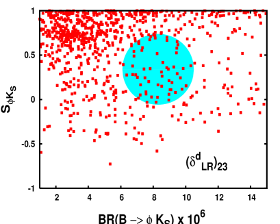
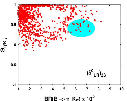
Figure 15: As in Fig.9, but for correlations of $S_{\phi K_{S}}$ versus $BR(B\to\phi K)$ (left) and $S_{\eta^{\prime}K_{S}}$ versus $BR(B\to\eta^{\prime}K)$ (right). Gluino contributions with one single mass insertion ${\left(\delta^{d}_{LR}\right)_{23}}$ has been considered.

In Fig. 15 we plot the CP asymmetries $S_{\phi K_{S}}$ versus $BR(B\to\phi K)$ and $S_{\eta^{\prime}K_{S}}$ versus $BR(B\to\eta^{\prime}K)$, where the area of colored ellipse corresponds as usual to the allowed experimental region for the correlations at $2\sigma$ level. We consider here the dominant gluino contribution due to ${\left(\delta^{d}_{LR}\right)_{23}}$ and scan over the other parameters as before. One can see from this figure that, gluino contribution can fit quite well inside the $2\sigma$ ellipse in both left and right plots. It is worth noticing that, gluino effects could also rise $BR(B\to\phi K)$ to very large values ($\simeq 1.5-2\times 10^{-5}$), which are outside the allowed region.

In the correlation between $S_{\eta^{\prime}K_{S}}$ and $BR(B\to\eta^{\prime}K)$, with just one mass insertion, SUSY contributions can explain the measured large $BR(B\to\eta^{\prime}K)$ and at the same time fit the 2$\sigma$ range for $S_{\eta^{\prime}K_{S}}$. As can be seen from this figure, for $S_{\eta^{\prime}K_{S}}$ within even 1$\sigma$ region, the $BR(B\to\eta^{\prime}K)$ can be large as $7\times 10^{-5}$. However, in this case some fine tuning between SUSY parameters is necessary.

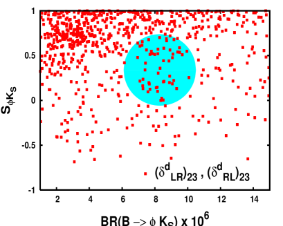
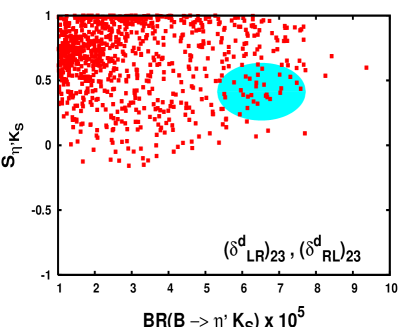
Figure 16: As in Fig. 15, but for gluino contributions with two mass insertions ${\left(\delta^{d}_{LR}\right)_{23}}$ and ${\left(\delta^{d}_{RL}\right)_{23}}$, with the assumption of ${\rm arg}[{\left(\delta^{d}_{LR}\right)_{23}}]={\rm arg}[{\left(\delta^{d}_{RL}\right)_{23}}]$.

In Fig. 16, we present the same correlations as in Fig. 15, but with two simultaneous contributions of mass insertions ${\left(\delta^{d}_{LR}\right)_{23}}$ and ${\left(\delta^{d}_{RL}\right)_{23}}$ in gluino sector. In this case, we can easily see that gluino scenario can saturate simultaneously both $S_{\phi K_{S}}$ and $BR(B\to\phi K)$ within their experimental ranges, covering also larger areas with respect to the ones in Fig. 15.

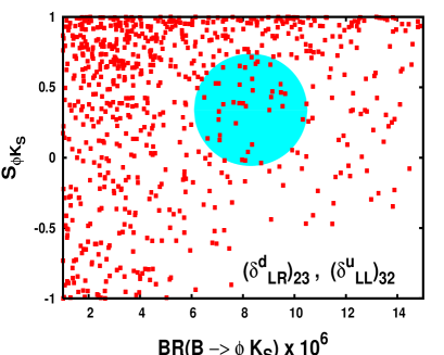
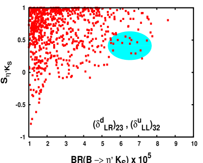
Figure 17: As in Fig. 15, but for gluino and chargino contributions with mass insertions ${\left(\delta^{d}_{LR}\right)_{23}}$ and ${\left(\delta^{u}_{LL}\right)_{32}}$, with the assumption of ${\rm arg}[{\left(\delta^{d}_{LR}\right)_{23}}]={\rm arg}[{\left(\delta^{u}_{LL}\right)_{32}}]$.

Finally, the combination from gluino and chargino exchanges on $BR(B\to\phi K)$ and $BR(B\to\eta^{\prime}K)$ versus the respective CP asymmetries, are shown in Fig. 17. We scan on the allowed range of the most relevant mass insertions for these two contributions: ${\left(\delta^{d}_{LR}\right)_{23}}$ (gluino) and ${\left(\delta^{u}_{LL}\right)_{32}}$ (chargino). We also vary the other parameters as in the previous cases. The message we can learn from these results is that both gluino (LR) and chargino (LL) contributions can easily accommodate the experimental results for the CP asymmetries and branching ratios of $BR(B\to\phi K)$ and $BR(B\to\eta^{\prime}K)$. As already stressed in section 4, this phenomenon is related to the fact that $b\to s\gamma$ constraints are more relaxed for chargino contributions at large $\tan\beta$, due to potentially destructive interferences of gluino and chargino amplitudes in $b\to s\gamma$ decay. The main difference emerging from results in Figs. 16 and 17, is that for the latter scenario large and negative values of asymmetry ($S_{\phi,\eta^{\prime}}\simeq-1$) can also be easily achieved, even though they are now outside the allowed experimental range.

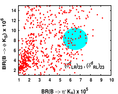
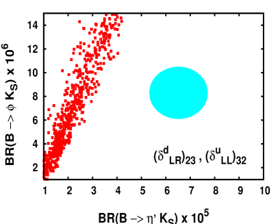
Figure 18: Correlations of $BR(B\to\phi K)$ versus $BR(B\to\eta^{\prime}K)$ for gluino contributions with two mass insertions ${\left(\delta^{d}_{LR}\right)_{23}}$ and ${\left(\delta^{d}_{RL}\right)_{23}}$ (left) and for gluino and chargino contributions with two mass insertions ${\left(\delta^{d}_{LR}\right)_{23}}$ and ${\left(\delta^{u}_{LL}\right)_{32}}$ (right). The $2\sigma$ constraints on $S_{\phi K_{S}}$ and $S_{\eta^{\prime}K_{S}}$ are applied.

It is crucial to see, if regions of points which fit inside the two $2\sigma$ ellipses in Figs. 16 and 17, actually correspond to the same SUSY configurations. For this purpose, in Fig. 18 we plot correlations of $BR(B\to\phi K)$ versus $BR(B\to\eta^{\prime}K)$ for the same scenarios considered in Figs. 16 and 17, where all points satisfy the constraints on $S_{\phi K_{S}}$ and $S_{\eta^{\prime}K_{S}}$ at $2\sigma$ level. As we can see from results in Fig. 18, only the scenario in which both LR and RL mass insertions in gluino exchanges contribute, can naturally enhance $BR(B\to\eta^{\prime}K)$ inside the allowed experimental range, while respecting all the other constraints on CP asymmetries. On the contrary, in the scenario in which both LR(gluino) and LL(chargino) are contributing, this enhancement is ruled out by simultaneous constraints on CP asymmetries.

As already mentioned, $BR(B\to\eta^{\prime}K)$ suffers from large theoretical uncertainties due to the peculiar structure of $\eta^{\prime}$ meson. Therefore, it is not a conservative approach to constrain NP models from the measurements of $BR(B\to\eta^{\prime}K)$, until the role of potential new mechanisms responsible of the enhancement of $BR(B\to\eta^{\prime}K)$ in the SM will be not completely clarified.

6 Direct CP asymmetry in $b\to s\gamma$ versus $S_{\phi(\eta^{\prime})K_{S}}$

In this section we analyze the correlation for SUSY predictions between the direct CP asymmetry $A_{CP}(b\to s\gamma)$ in $b\to s\gamma~{}$decay and the other ones in $B\to\phi(\eta^{\prime})K_{S}$. The CP asymmetry in $b\to s\gamma~{}$is measured in the inclusive radiative decay of $B\to X_{s}\gamma$ by the quantity

$$A_{CP}(b\to s\gamma)=\frac{\Gamma(\bar{B}\to X_{s}\gamma)-\Gamma(B\to X_{\bar{s}}\gamma)}{\Gamma(\bar{B}\to X_{s}\gamma)+\Gamma(B\to X_{\bar{s}}\gamma)}.$$ (67)

The SM prediction for $A_{CP}(b\to s\gamma)$ is very small, less than $1\%$ in magnitude, but known with high precision [46]. Indeed, inclusive decay rates of B mesons are free from large theoretical uncertainties since they can be reliably calculated in QCD using the OPE. Thus, the observation of sizeable effects in $A_{CP}(b\to s\gamma)$ would be a clean signal of new physics. In particular, large asymmetries are expected in models with enhanced chromo-magnetic dipole operators, like for instance supersymmetric models [46].

The most recent result reported by BaBar collaboration for $A_{CP}(b\to s\gamma)$ is [60]

$$A_{CP}^{b\to s\gamma}=0.025\pm 0.050~{}(stat.)~{}\pm 0.015~{}(syst.),$$ (68)

which corresponds to the following allowed range at $90\%$ confidence level:

$$-6\%<A_{CP}^{b\to s\gamma}<11\%~{}.$$ (69)

Clearly, the present experimental sensitivity is not accurate enough to strongly constrain the SM predictions at percent level.

Recently it has been shown that the SUSY contribution to the CP asymmetry in the $b\to s\gamma~{}$decay, even with the inclusion of experimental constraints on electric dipole moments and branching ratio of $B\to X_{s}\gamma$, could be much larger than the SM expectation [36] . Therefore, in the light of present experimental results, it would be challenging to analyze the SUSY predictions for the correlation between $A_{CP}(b\to s\gamma)$ and $S_{\phi,(\eta^{\prime})K_{S}}$, since in SUSY models these asymmetries are strongly correlated.

The relevant operators of the effective Hamiltonian in Eq.(7) that play a role in $A_{CP}(b\to s\gamma)$, are given by $Q_{2}$, $Q_{7\gamma},Q_{8g}$. We remind here that $Q_{2}$, defined in Eqs.(8), is the usual current-current operator induced at tree-level. Then, the expression for $A_{CP}(b\to s\gamma)$ at the NLO accuracy, is given by [46]

$$A_{CP}(b\to s\gamma) = \frac{\alpha_{s}(m_{b})}{|C_{7\gamma}|^{2}}\Bigg{\{}\frac{40}{81}{\rm Im}\left[C_{2}C_{7\gamma}^{\star}\right]-\frac{8z}{9}\left[v(z)+b(z,\delta)\right]\,{\rm Im}\left[\left(1+\epsilon_{s}\right)C_{2}C_{7\gamma}^{\star}\right]$$ (70)

$$- \frac{4}{9}{\rm Im}\left[C_{8g}C_{7\gamma}^{\star}\right]+\frac{8z}{27}b(z,\delta){\rm Im}\left[\left(1+\epsilon_{s}\right)C_{2}C_{8g}^{\star}\right]\Bigg{\}},$$

where $z=(m_{c}/m_{b})^{2}$ and $v(z)$ is [46]

$$v(z)=\left(5+\ln z+\ln^{2}z-\frac{\pi^{2}}{3}\right)+\left(\ln^{2}z-\frac{\pi^{2}}{3}\right)z+\left(\frac{28}{9}-\frac{4}{3}\ln z\right)z^{2}+\mathcal{O}(z^{3}).$$ (71)

The function $b(z,\delta)$ is defined as $b(z,\delta)=g(z,1)-g(z,1-\delta)$, where the parameter $\delta$ is related to the experimental cut on the photon energy, $E_{\gamma}>(1-\delta)m_{b}/2$, and finally $g(z,y)$ is given by

$$g(z,y)=\theta(y-4z)\left\{\left(y^{2}-4yz+6z^{2}\right)\ln\left(\sqrt{\frac{y}{4z}}+\sqrt{\frac{y}{4z}-1}\right)-\frac{3y(y-2z)}{4}\sqrt{1-\frac{4z}{y}}\right\}.$$ (72)

In the SM, the Wilson coefficients $C_{2}$, $C_{7\gamma}$, and $C_{8g}$ are real, in particular $C_{2}^{SM}\simeq 1.08$, $C_{7\gamma}=-0.318$, and $C_{8g}=-0.151$, so that the only source of CP violation comes from the $\epsilon_{s}$ parameter inside Eq.(70) which is defined in terms of the CKM matrix elements as

$$\epsilon_{s}=\frac{V_{us}^{\star}V_{ub}}{V_{ts}^{\star}V_{tb}}\approx\lambda^{2}(i\eta-\rho)\sim{\cal O}(10^{-2})\,.$$ (73)

In general SUSY models, $C_{7\gamma}$ and $C_{8g}$ may be complex, and the corresponding phase can provide the dominant CP violating source to $A_{CP}^{b\to s\gamma}$. In MIA framework, the SUSY contributions to the Wilson coefficients $C_{7\gamma}$ and $C_{8g}$ are given in terms of $(\delta^{d}_{AB})_{23}$ (for gluino) and $(\delta^{u}_{AB})_{32}$ (for chargino). Therefore, the SUSY phase in these mass insertions is the only source of CP violation in this process. As pointed out in previous sections, in general SUSY models, effects induced by the dipole operators $\tilde{Q}_{7\gamma}$ and $\tilde{Q}_{8g}$, which have opposite chirality to $Q_{7\gamma}$ and $Q_{8g}$, are non-negligible. In the MSSM these contributions are suppressed by terms of order ${\cal O}(m_{s}/m_{b})$ due to the universality of the $A$–terms. However, in general models one should take them into account, since they might be of the same order than $C_{7\gamma}$ and $C_{8g}$. Denoting by $\tilde{C}_{7\gamma}$ and $\tilde{C}_{8g}$ the Wilson coefficients multiplying the new operators $\tilde{Q}_{7\gamma}$ and $\tilde{Q}_{8g}$, the expression for the asymmetry in Eq.(70) will be modified by making the replacement

$$C_{i}C_{j}^{*}\to C_{i}C_{j}^{*}+\tilde{C}_{i}\tilde{C}_{j}^{*}.$$ (74)

Notice that, since $\tilde{C}_{2}=0$, the only modification in the numerator of Eq.(70) is due to the new term $\tilde{C}_{7\gamma}\tilde{C}_{8g}$. However, if only one single mass insertion is taken into account, both $\tilde{C}_{7\gamma}$ and $\tilde{C}_{8g}$ will be proportional to the same mass insertion, and therefore ${\rm Im}\left(\tilde{C}_{8g}\tilde{C}^{\star}_{7\gamma}\right)=0$. Therefore, the effects of these new operators will enter only through $\tilde{C}_{7\gamma}$ in the denominator, by means of the shift $|C_{7\gamma}|^{2}\to|C_{7\gamma}|^{2}+|\tilde{C}_{7\gamma}|^{2}$.

It is worth mentioning that in the scenarios dominated by one single mass insertion, the leading SUSY contribution to the CP asymmetry $A_{CP}(b\to s\gamma)$ is due to the $C_{7\gamma}$. This can be understood as follows. Using our previous inputs for charm and bottom masses and also assuming, for instance, an energy resolution $\delta\simeq 0.3$ so that $b(z,\delta)\simeq 0.17$, Eq.(70) can be written as

$$A_{CP}(b\to s\gamma)\simeq\frac{\alpha_{s}(m_{b})}{|C_{7\gamma}|^{2}}\left(0.045~{}{\rm Im}[C_{7\gamma}^{*}]-0.44~{}{\rm Im}[C_{7\gamma}C^{*}_{8g}]+0.006~{}{\rm Im}[C_{8g}^{*}]\right).$$ (75)

We remind here that the low energy coefficients $C_{7\gamma}$ and $C^{*}_{8g}$ at $\mu_{b}$ scale are related to the high energy ones by

$$C_{7\gamma}^{SUSY}(m_{b})\simeq 0.66~{}C_{7\gamma}^{SUSY}(\mu_{W})+0.09~{}C_{8g}^{SUSY}(\mu_{W}),$$ (76)

$$C_{8g}^{SUSY}(m_{b})\simeq 0.69~{}C_{8g}^{SUSY}(\mu_{W}).$$ (77)

As shown in section 2, the kind of mass insertions that will appear in $C_{7\gamma}(\mu_{W})$ are the same that determine $C_{8g}(\mu_{W})$. In the case of SUSY contribution from one single mass insertion, both $C_{7\gamma}(\mu_{b})$ and $C^{*}_{8g}(\mu_{b})$ will acquire the same phase and so the second term in Eq.(70) identically vanishes.

In conclusion, the relevant mass insertions contributing to $A_{CP}(b\to s\gamma)$ give also the dominant effects in $S_{\phi K_{S}}$ and $S_{\eta^{\prime}K_{S}}$. Therefore, it is expected that these three CP asymmetries should be highly correlated, since all of them depend on the same source of SUSY CP violation.

In Fig. 19 we plot the correlations between $S_{K_{S}\phi}$ and $A_{CP}(b\to s\gamma)$ and also $S_{\eta^{\prime}K_{S}}$ and $A_{CP}(b\to s\gamma)$ for gluino exchanges with one mass insertion, namely ${\left(\delta^{d}_{LR}\right)_{23}}$. As we can see from results in Fig. 19, a specific trend emerges from this scenario. The simultaneous combination of $S_{\phi K_{S}}$ and $S_{\eta^{\prime}K_{S}}$ constraints, favors the SUSY predictions to be in the region of positive values of $A_{CP}(b\to s\gamma)$ asymmetry. As shown in Fig. 20, analogous results are also obtained when two mass insertions in gluino sector are taken simultaneously, namely ${\left(\delta^{d}_{LR}\right)_{23}}$ and ${\left(\delta^{d}_{LR}\right)_{23}}$. However, in this case also negative values of $A_{CP}^{b\to s\gamma}$ are allowed. Although these points are favored by $S_{\phi K_{S}}$, they are disfavored by $S_{\eta^{\prime}K_{S}}$.

Finally, in Fig. 21 we show our results for two mass insertions ${\left(\delta^{d}_{LR}\right)_{23}}$ and ${\left(\delta^{u}_{LL}\right)_{32}}$ with both gluino and chargino exchanges. In this case we see that $S_{\phi K_{S}}$ constraints do not set any restriction on $A_{CP}(b\to s\gamma)$, and also large and positive values of $A_{CP}(b\to s\gamma)$ asymmetry can be achieved. However, by imposing the constraints on $S_{\eta^{\prime}K_{S}}$, see plot on the right side of Fig. 21, the region of negative $A_{CP}(b\to s\gamma)$ is disfavored in this scenario as well.

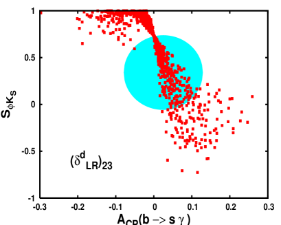
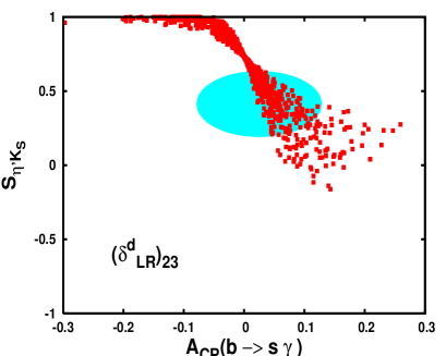
Figure 19: Correlations of $S_{\phi K_{S}}$ versus $A_{CP}(b\to s\gamma)$ (left) and $S_{\eta^{\prime}K_{S}}$ versus $A_{CP}(b\to s\gamma)$ (right), for gluino contributions with one single mass insertion ${\left(\delta^{d}_{LR}\right)_{23}}$.

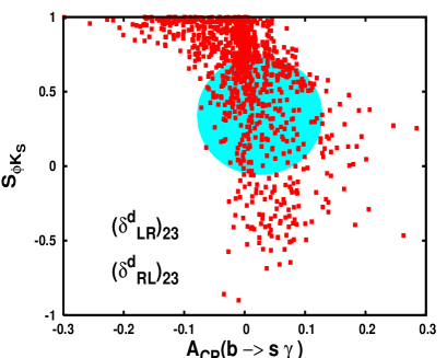
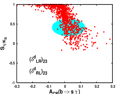
Figure 20: As in Fig. 19, but for gluino contributions with two mass insertions ${\left(\delta^{d}_{LR}\right)_{23}}$ and ${\left(\delta^{d}_{RL}\right)_{23}}$.

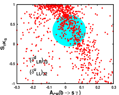
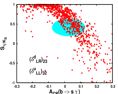
Figure 21: As in Fig. 19, but for gluino and chargino contributions with mass insertions ${\left(\delta^{d}_{LR}\right)_{23}}$ and ${\left(\delta^{u}_{LL}\right)_{32}}$ respectively.

7 Conclusions

The $B$-meson decays to $\phi K$, $\eta^{\prime}K$, and to $X_{S}\gamma$ provide a clean window to the physics beyond the SM. In this paper we have systematically analyzed the supersymmetric contributions to the CP asymmetries and the branching ratios of these processes in a model independent way. The relevant SUSY contributions in the $b\to s$ transitions, namely chargino and gluino exchanges in box and penguin diagrams, have been considered by using the mass insertion method.

We have provided analytical expressions for all the relevant Wilson coefficients. Both naive factorization and QCD factorization approximation to determine the hadronic matrix elements have been employed. We showed that the SUSY predictions for the mixing CP asymmetry of $S_{\phi K_{S}}$ and $S_{\eta^{\prime}K_{S}}$ are not very sensitive to the kind of approximation adopted for evaluating hadronic matrix elements.

We found that due to the stringent constraints from the experimental measurements of $BR(b\to s\gamma)$, the scenario with pure chargino exchanges cannot give large and negative values for CP asymmetry $S_{\phi K_{S}}$. Indeed, by combining present experimental constraints on $S_{\phi K_{S}}$ and $S_{\eta^{\prime}K_{S}}$ asymmetries at $2\sigma$ level, pure chargino contributions can be almost ruled out. On the other hand, it is quite possible for gluino exchanges to account for $S_{\phi K_{S}}$ and $S_{\eta^{\prime}K_{S}}$ at the same time. Interestingly, we have shown that the charged Higgs, if not too heavy, may change the chargino and gluino contributions to enhance the CP asymmetries considerably.

The branching ratios of these decays have also been considered. It has been noticed that the $\rho$ parameter is strictly bounded by the $B\to\phi K$ branching ratio, and this influences strongly the possible SUSY contributions to the asymmetries. Investigating the correlations between CP asymmetries and branching ratios, pointed out that the most favored SUSY scenarios, which easily satisfy all the experimental results, are the ones with inclusion of two mass insertions. In particular, a pure gluino dominated scenario, in which both $LR$ and $RL$ mass insertions are contributing and the one in which both gluino and chargino contribute with $LR$ and $LL$ mass insertions in down- and up-squark sectors, respectively. In the latter scenario we show that chargino exchanges provide sizeable effects. This is due to the fact that $b\to s\gamma$ constraints could be relaxed by potentially destructive interferences between gluino and chargino amplitudes. Finally, it is remarkable to notice that in the scenario in which both LR and RL down squark mass insertions dominate, the observed large enhancement of $BR(B\to\eta^{\prime}K)$ could be naturally explained, while respecting all the other experimental constraints on CP asymmetries.

We also discussed the correlations between the CP asymmetries of these processes and the direct CP asymmetry in $b\to s\gamma$ decay. In this case, we found that the general trend of SUSY models, satisfying all the experimental constraints, strongly favors large and positive contributions to $b\to s\gamma$ asymmetry.

More precise measurements would certainly allow us to draw more definite conclusions on the SUSY models that can accommodate these data.

Acknowledgments

The authors thank Debrupa Chakraverty for her efforts in the initial stages of this work. We would like to thank G. D’Agostini, E. Kou, and K. Österberg for very useful discussions. E.G. acknowledges the CERN PH-TH division and IPPP, CPT of Durham University for their kind hospitality during the preparation of this work. The authors appreciate the financial support from the Academy of Finland (project numbers 104368 and 54023) and from the Associate Scheme of ICTP.

Appendix

Appendix A Chargino contributions in MIA

Here we provide the expressions for chargino contributions, at leading order in MIA, to the $R_{F}^{AB}$ quantities in Eq.(15), where $F$ refers to $D,E,C,B_{(u,d)}$, and $M_{\gamma,g}$ [11].

$$R_{D}^{LL} = \sum_{i=1,2}\,|V_{i1}|^{2}\,x_{{\scriptscriptstyle W}i}\,P_{D}(x_{i})$$

$$R_{D}^{RL} = -\sum_{i=1,2}V_{i2}^{\star}V_{i1}\,x_{{\scriptscriptstyle W}i}\,P_{D}(x_{i})$$

$$R_{D}^{RR} = \sum_{i=1,2}\,|V_{i2}|^{2}\,x_{{\scriptscriptstyle W}i}\,P_{D}(x_{i})$$

$$R_{D}^{LR} = \left(R_{D}^{RL}\right)^{\star}$$

$$R_{E}^{LL} = \sum_{i=1,2}\,|V_{i1}|^{2}\,x_{{\scriptscriptstyle W}i}\,P_{E}(x_{i})$$

$$R_{E}^{RL} = -\sum_{i=1,2}V_{i2}^{\star}V_{i1}\,x_{{\scriptscriptstyle W}i}\,P_{E}(x_{i})$$

$$R_{E}^{RR} = \sum_{i=1,2}\,|V_{i2}|^{2}\,x_{{\scriptscriptstyle W}i}\,P_{E}(x_{i})$$

$$R_{E}^{LR} = \left(R_{E}^{RL}\right)^{\star}$$

$$R_{C}^{LL} = \sum_{i=1,2}|V_{i1}|^{2}\,P_{C}^{(0)}(\bar{x}_{i})+\sum_{i,j=1,2}\left[U_{i1}V_{i1}U_{j1}^{\star}V_{j1}^{\star}\,P_{C}^{(2)}(x_{i},x_{j})\right.$$

$$+ \left.|V_{i1}|^{2}|V_{j1}|^{2}\left(\frac{1}{8}-P_{C}^{(1)}(x_{i},x_{j})\right)\right]$$

$$R_{C}^{RL} = -\frac{1}{2}\sum_{i=1,2}\,V_{i2}^{\star}V_{i1}\,P_{C}^{(0)}(\bar{x}_{i})-\sum_{i,j=1,2}\,V_{j2}^{\star}V_{i1}\left(U_{i1}U_{j1}^{\star}\,P_{C}^{(2)}(x_{i},x_{j})\right.$$

$$+ \left.V_{i1}^{\star}V_{j1}\,P_{C}^{(1)}(x_{i},x_{j})\right)$$

$$R_{C}^{LR} = \left(R_{C}^{RL}\right)^{\star},$$

$$R_{C}^{RR} = \sum_{i,j=1,2}\,V_{j2}^{\star}V_{i2}\left(U_{i1}U_{j1}^{\star}\,P_{C}^{(2)}(x_{i},x_{j})+V_{i1}^{\star}V_{j1}\,P_{C}^{(1)}(x_{i},x_{j})\right)$$

$$R_{B_{u}}^{LL} = 2\sum_{i,j=1,2}\,V_{i1}V_{j1}^{\star}U_{i1}U_{j1}^{\star}\,x_{Wj}\sqrt{x_{ij}}~{}P_{B}^{u}(\bar{x}_{j},x_{ij})$$

$$R_{B_{u}}^{RL} = -2\sum_{i,j=1,2}\,V_{i1}V_{j2}^{\star}U_{i1}U_{j1}^{\star}\,x_{Wj}\sqrt{x_{ij}}~{}P_{B}^{u}(\bar{x}_{j},x_{ij})$$

$$R_{B_{u}}^{LR} = \left(R_{B_{u}}^{RL}\right)^{\star}$$

$$R_{B_{u}}^{RR} = 2\sum_{i,j=1,2}\,V_{i2}V_{j2}^{\star}U_{i1}U_{j1}^{\star}\,x_{Wj}\sqrt{x_{ij}}~{}P_{B}^{u}(\bar{x}_{j},x_{ij})$$

$$R_{B_{d}}^{LL} = \sum_{i,j=1,2}\,|V_{i1}|^{2}|V_{j1}|^{2}\,x_{Wj}\,P_{B}^{d}(\bar{x}_{j},x_{ij})$$

$$R_{B_{d}}^{RL} = -\sum_{i,j=1,2}\,V_{i2}^{\star}V_{i1}|V_{j1}|^{2}\,x_{Wj}\,P_{B}^{d}(\bar{x}_{j},x_{ij})$$

$$R_{B_{d}}^{LR} = \left(R_{B_{d}}^{RL}\right)^{\star}$$

$$R_{B_{d}}^{RR} = \sum_{i,j=1,2}\,V_{i2}^{\star}V_{i1}V_{j1}^{\star}V_{j2}\,x_{Wj}\,P_{B}^{d}(\bar{x}_{j},x_{ij})$$

$$R_{M_{\gamma,g}}^{LL} = \sum_{i}|V_{i1}|^{2}\,x_{Wi}\,P_{M_{\gamma,g}}^{LL}(x_{i})-Y_{b}\sum_{i}V_{i1}U_{i2}\,x_{Wi}\,\frac{m_{\chi_{i}}}{m_{b}}P_{M_{\gamma,g}}^{LR}(x_{i})$$

$$R_{M_{\gamma,g}}^{LR} = -\sum_{i}V_{i1}^{\star}V_{i2}\,x_{Wi}\,P_{M_{\gamma,g}}^{LL}(x_{i})+Y_{b}\sum_{i}V_{i2}U_{i2}\,x_{Wi}\,\frac{m_{\chi_{i}}}{m_{b}}P_{M_{\gamma,g}}^{LR}(x_{i})$$

$$R_{M_{\gamma,g}}^{RL} = -\sum_{i}V_{i1}V_{i2}^{\star}\,x_{Wi}\,P_{M_{\gamma,g}}^{LL}(x_{i})$$

$$R_{M_{\gamma,g}}^{RR} = \sum_{i}|V_{i2}|^{2}\,x_{Wi}\,P_{M_{\gamma,g}}^{LL}(x_{i})\,.$$ (78)

Regarding the $R_{F}^{0}$ terms at the zero order in mass insertion, we have

$$R_{D}^{0} = 2x_{W}\sum_{i=1,2}|V_{i2}|^{2}D_{\chi}(x_{i})$$

$$R_{E}^{0} = 2x_{W}\sum_{i=1,2}|V_{i2}|^{2}E_{\chi}(x_{i})$$

$$R_{C}^{0} = 2\sum_{i,j=1,2}U_{i1}U^{\star}_{j1}V_{i2}V^{\star}_{j2}C_{\chi}^{(2)}(x_{i},x_{j})$$

$$R_{B_{d}}^{0} = -\frac{1}{2}\sum_{i,j=1,2}x_{Wj}V_{i2}^{\star}V_{i1}V_{j1}^{\star}V_{j2}B^{(d)}_{\chi}(\bar{x}_{j},\bar{x_{j}},x_{ij})$$

$$R_{B_{u}}^{0} = \sum_{i,j=1,2}x_{Wj}V_{i2}V_{j2}^{\star}U_{i1}^{\star}U_{j1}^{\star}B^{(u)}_{\chi}(\bar{x}_{j},\bar{x_{j}},x_{ij})$$

$$R_{M_{\gamma}}^{0} = -x_{W}\sum_{i=1,2}|V_{i2}|^{2}\left(F_{1}(x_{i})+\frac{2}{3}F_{2}(x_{i})\right)$$

$$R_{M_{g}}^{0} = -x_{W}\sum_{i=1,2}|V_{i2}|^{2}F_{2}(x_{i})$$ (79)

where $Y_{b}$ is the Yukawa coupling of bottom quark, $x_{{\scriptscriptstyle W}i}\equiv m_{W}^{2}/m_{\chi_{i}}^{2}$, $x_{{\scriptscriptstyle W}}\equiv m_{W}^{2}/\tilde{m}^{2}$, $x_{i}\equiv m_{\chi_{i}}^{2}/\tilde{m}^{2}$, $\bar{x}_{i}\equiv\tilde{m}^{2}/m_{\chi_{i}}^{2}$, and $x_{ij}\equiv m_{\chi_{i}}^{2}/m_{\chi_{j}}^{2}$. The chargino mixing matrices $U$ and $V$, are defined in Eq.(13). The loop functions of penguin $P_{D,E,C}$, $D_{\chi},E_{\chi},C_{\chi}$, box $B^{(u,d,\tilde{g})}$, $P_{B}^{(u,d,\tilde{g})}$, and magnetic and chromo-magnetic penguin diagrams $F_{1,2}$, $P_{M_{\gamma,g}}^{LL}$, $P_{M_{\gamma,g}}^{LR}$ are reported in appendix C.

Appendix B Chargino contributions in MIA for the light $\tilde{t}_{R}$ case

In this appendix we provide the relevant formulas for the case in which the mass of the stop-right ($m^{2}_{{\tilde{t}}_{R}}$) is lighter than the average squark mass $\tilde{m}^{2}$. We recall here that this will modify only the expressions of $R_{F}^{RL}$, $R_{F}^{RR}$, and $R_{F}^{0}$, since the light stop right does not affect $R_{F}^{LL}$. In the case of $R_{D,E,C}^{RR}$ and $R_{D,E,C}^{0}$ the functional forms of $R_{D,E,C}^{RR}$ and $R_{D,E,C}^{0}$ remain unchanged, while the arguments of the functions involved are changed as $x_{W}\to x_{Wt}$, $x_{i}\to x_{it}$, and ${\bar{x}}_{i}\to{\bar{x}}_{it}$, where $x_{Wt}\equiv m_{W}^{2}/m^{2}_{\tilde{t}_{R}}$, $x_{it}\equiv m_{\chi_{i}}^{2}/{m^{2}_{{\tilde{t}}_{R}}}$, ${\bar{x}_{it}}\equiv{m^{2}_{{\tilde{t}}_{R}}}/m_{\chi_{i}}^{2}$. Regarding the box-type contributions $R_{B_{u,d}}^{RR}$ and $R_{B_{u,d}}^{0}$, the functions $P_{B}^{(u,d)}$ and $B_{\chi}^{(u,d)}$ appearing there should be replaced as follows

$$P_{B}^{(u,d)}(\bar{x}_{j},x_{ij}) \to \bar{P}_{B}^{(u,d)}(\bar{x}_{jt},\bar{x}_{j},x_{ij})$$

$$B^{(u,d)}_{\chi}(\bar{x}_{j},\bar{x}_{j},x_{ij}) \to B^{(u,d)}_{\chi}(\bar{x}_{jt},\bar{x}_{j},x_{ij})\,,$$ (80)

where

$$\bar{P}_{B}^{(u,d)}(x,y,z)=\frac{1}{2}x\frac{\partial}{\partial x}B^{(u,d)}_{\chi}(x,y,z)\,.$$ (81)

In the case of $R_{F}^{LR}$ and $R_{F}^{RL}$ the analytical expression of loop functions of penguin $P_{D,E,C}$, box $P_{B}^{(u,d)}$, and magnetic and chromo-magnetic penguin diagrams $P_{M_{\gamma,g}}^{LL}$ and $P_{M_{\gamma,g}}^{LR}$ respectively, should be replaced with the following ones

$$P_{D,E}(x_{i}) \to P_{D,E}(x_{i},x_{it})$$

$$P_{C}^{0}(\bar{x}_{i}) \to P_{C}^{0}(\bar{x}_{i},\bar{x}_{it})$$

$$P_{C}^{(1,2)}(x_{i},x_{j}) \to P_{C}^{(1,2)}(x_{i},x_{it},x_{j},x_{jt})$$

$$P_{B}^{(u,d)}({\bar{x}}_{j},x_{ij}) \to P_{B}^{(u,d)}({\bar{x}}_{j},{\bar{x}}_{jt},x_{ij})$$ (82)

where

$$P_{D}(x_{i},x_{it}) = {2\over{(x_{t}-1)}}\left[x_{it}D_{\chi}(x_{it})-x_{i}D_{\chi}(x_{i})\right]$$

$$P_{E}(x_{i},x_{it}) = {2\over{(x_{t}-1)}}\left[x_{it}E_{\chi}(x_{it})-x_{i}E_{\chi}(x_{i})\right]$$

$$P_{C}^{(1,2)}(x_{i},x_{it},x_{j},x_{jt}) = {2\over{(x_{t}-1)}}\left[C_{\chi}^{(1,2)}(x_{jt},x_{it})-C_{\chi}^{(1,2)}(x_{j},x_{i})\right]$$

$$P_{C}^{(0)}({\bar{x}}_{i},{\bar{x}}_{it}) = {4\over{(x_{t}-1)}}\left[C_{\chi}^{(1)}({\bar{x}}_{it},{\bar{x}}_{i})-C_{\chi}^{(1)}({\bar{x}}_{i},{\bar{x}}_{i})\right]$$

$$P_{B}^{(u)}({\bar{x}}_{j},{\bar{x}}_{jt},x_{ij}) = {1\over{2(x_{t}-1)}}\left[B_{\chi}^{(u)}({\bar{x}}_{jt},{\bar{x}}_{j},x_{ij})-B_{\chi}^{(u)}({\bar{x}}_{j},{\bar{x}}_{j},x_{ij})\right]$$

$$P_{B}^{(d)}({\bar{x}}_{j},{\bar{x}}_{jt},x_{ij}) = -{1\over{2(x_{t}-1)}}\left[B_{\chi}^{(d)}({\bar{x}}_{jt},{\bar{x}}_{j},x_{ij})-B_{\chi}^{(d)}({\bar{x}}_{j},{\bar{x}}_{j},x_{ij})\right]$$

$$P_{M_{\gamma}}^{LL}(x_{i},x_{it}) = {1\over{(x_{t}-1)}}\left[x_{it}\left(F_{1}(x_{it})+\frac{2}{3}F_{2}(x_{it})\right)-x_{i}\left(F_{1}(x_{i})+\frac{2}{3}F_{2}(x_{i})\right)\right]$$

$$P_{M_{\gamma}}^{LR}(x_{i},x_{it}) = {1\over{(x_{t}-1)}}\left[x_{it}\left(F_{3}(x_{it})+\frac{2}{3}F_{4}(x_{it})\right)-x_{i}\left(F_{3}(x_{i})+\frac{2}{3}F_{4}(x_{i})\right)\right]$$

$$P_{M_{g}}^{LL}(x_{i},x_{it}) = {1\over{(x_{t}-1)}}\left[x_{it}F_{2}(x_{it})-x_{i}F_{2}(x_{i})\right]$$

$$P_{M_{g}}^{LR}(x_{i},x_{it}) = {1\over{(x_{t}-1)}}\left[x_{it}F_{4}(x_{it})-x_{i}F_{4}(x_{i})\right]\,.$$ (83)

The expressions for the loop functions involved in Eqs.(81) and (83) can be found in Appendix C.

Appendix C Basic SM and SUSY Loop functions

Here we report the loop functions entering in the SM and SUSY diagrams at 1-loop.

• SM functions

  $${\rm D}(x) = \frac{x^{2}\left(25-19x\right)}{36\left(x-1\right)^{3}}+\frac{\left(-3x^{4}+30x^{3}-54x^{2}+32x-8\right)}{18\left(x-1\right)^{4}}\log{x}$$

  $${\rm C}(x) = \frac{x\left(x-6\right)}{8\left(x-1\right)}+\frac{x\left(3x+2\right)}{8\left(x-1\right)^{2}}\log{x}$$

  $${\rm E}(x) = \frac{x\left(x^{2}+11x-18\right)}{12\left(x-1\right)^{3}}+\frac{\left(-9x^{2}+16x-4\right)}{6\left(x-1\right)^{4}}\log{x}$$

  $${\rm B}(x) = -\frac{x}{4(x-1)}+\frac{x}{4(x-1)^{2}}\log{x}$$ (84)

• Charged Higgs functions

  $${\rm D_{H}}(x) = \frac{x\left(47x^{2}-79x+38\right)}{108\left(x-1\right)^{3}}+\frac{x\left(-3x^{2}+6x-4\right)}{18\left(x-1\right)^{4}}\log{x}$$

  $${\rm C_{H}}(x) = -\frac{1}{2}{\rm B}(x)$$

  $${\rm E_{H}}(x) = \frac{x\left(7x^{2}-29x+16\right)}{36\left(x-1\right)^{3}}+\frac{x\left(3x-2\right)}{6\left(x-1\right)^{4}}\log{x}$$ (85)

• Chargino functions in MIA

  $$P_{D}(x) = {\frac{2\,x\,\left(-22+60\,x-45\,{x^{2}}+4\,{x^{3}}+3\,{x^{4}}-3\,\left(3-9\,{x^{2}}+4\,{x^{3}}\right)\,\log{x}\right)}{27\,{{\left(1-x\right)}^{5}}}}$$

  $$P_{E}(x) = {\frac{x\,\left(-1+6\,x-18\,{x^{2}}+10\,{x^{3}}+3\,{x^{4}}-12\,{x^{3}}\,\log{x}\right)}{9\,{{\left(1-x\right)}^{5}}}}$$

  $$P_{C}^{(0)}(x) = {\frac{x\,\left(3-4\,x+{x^{2}}+2\,\log{x}\right)}{8\,{{\left(1-x\right)}^{3}}}}$$

  $$P_{C}^{(1)}(x,y) = \frac{1}{8\left(x-y\right)}\left[\frac{x^{2}\left(x-1-\log{x}\right)}{(x-1)^{2}}-\frac{y^{2}\left(y-1-\log{y}\right)}{(y-1)^{2}}\right]$$

  $$P_{C}^{(2)}(x,y) = \frac{\sqrt{xy}}{4\left(x-y\right)}\left[\frac{x\left(x-1-\log{x}\right)}{(x-1)^{2}}-\frac{y\left(y-1-\log{y}\right)}{(y-1)^{2}}\right]$$

  $$P_{B}^{u}(x,y) = {\frac{-y-x\,\left(1-3\,x+y\right)}{4\,{{\left(x-1\right)}^{2}}\,{{\left(x-y\right)}^{2}}}}-{\frac{x\,\left({x^{3}}+y-3\,x\,y+{y^{2}}\right)\,\log{x}}{2\,{{\left(x-1\right)}^{3}}\,{{\left(x-y\right)}^{3}}}}$$

  $$+ {\frac{x\,y\,\log{y}}{2\,{{\left(x-y\right)}^{3}}\,\left(y-1\right)}}$$

  $$P_{B}^{d}(x,y) = -{\frac{x\,\left(3\,y-x\,\left(1+x+y\right)\right)}{4\,{{\left(x-1\right)}^{2}}\,{{\left(x-y\right)}^{2}}}}-{\frac{x\,\left({x^{3}}+\left(x-3\right)\,{x^{2}}\,y+{y^{2}}\right)\,\log{x}}{2\,{{\left(x-1\right)}^{3}}\,{{\left(x-y\right)}^{3}}}}$$

  $$+ {\frac{x\,{y^{2}}\,\log{y}}{2\,{{\left(x-y\right)}^{3}}\,\left(y-1\right)}}$$

  $$P_{M_{\gamma}}^{LL}(x) = \frac{x\left(-2-9x+18x^{2}-7x^{3}+3x\left(x^{2}-3\right)\log{x}\right)}{9\left(1-x\right)^{5}}$$

  $$P_{M_{\gamma}}^{LR}(x) = \frac{x\left(13-20x+7x^{2}+\left(6+4x-4x^{2}\right)\log{x}\right)}{6\left(1-x\right)^{4}}$$

  $$P_{M_{g}}^{LL}(x) = \frac{x\left(-1+9x+9x^{2}-17x^{3}+6x^{2}\left(3+x\right)\log{x}\right)}{12\left(1-x\right)^{5}}$$

  $$P_{M_{g}}^{LR}(x) = \frac{x\left(-1-4x+5x^{2}-2x\left(2+x\right)\log{x}\right)}{2\left(1-x\right)^{4}}$$ (86)

• Chargino functions in MIA with a light $\tilde{t}_{R}$

  $$D_{\chi}(x) = \frac{\left(-43x^{2}+101x-52\right)}{108\left(x-1\right)^{3}}+\frac{\left(2x^{3}-9x+6\right)}{18\left(x-1\right)^{4}}\log{x}$$

  $$C_{\chi}^{(1)}(x,y) = \frac{1}{16\left(y-x\right)}\left[\frac{x^{2}}{x-1}\log{x}-\frac{y^{2}}{y-1}\log{y}\right]$$

  $$C_{\chi}^{(2)}(x,y) = \frac{\sqrt{xy}}{8\left(y-x\right)}\left[\frac{x}{x-1}\log{x}-\frac{y}{y-1}\log{y}\right]$$

  $$E_{\chi}(x) = \frac{\left(-11x^{2}+7x-2\right)}{36\left(x-1\right)^{3}}+\frac{x^{3}}{6\left(x-1\right)^{4}}\log{x}$$

  $$B^{(u)}_{\chi}(x,y,z) = -\Big{[}F(x,y,z)+F(y,z,x)+F(z,x,y)\Big{]}$$

  $$B^{(d)}_{\chi}(x,y,z) = xF(x,y,z)+yF(y,z,x)+zF(z,x,y)$$

  $$F(x,y,z) = \frac{x\log{x}}{(x-1)(x-y)(x-z)}$$

  $$F_{1}(x) = \frac{\left(x^{3}-6x^{2}+3x+2+6x\log{x}\right)}{12\left(x-1\right)^{4}}$$

  $$F_{2}(x) = \frac{\left(2x^{3}+3x^{2}-6x+1-6x^{2}\log{x}\right)}{12\left(x-1\right)^{4}}$$

  $$F_{3}(x) = \frac{\left(x^{2}-4x+3+2\log{x}\right)}{2\left(x-1\right)^{3}}$$

  $$F_{4}(x) = \frac{\left(x^{2}-1+2x\log{x}\right)}{2\left(x-1\right)^{3}}$$ (87)

• Gluino functions in MIA

  $${\mbox{P}}_{1}(x) = {{1-6\,x+18\,{x^{2}}-10\,{x^{3}}-3\,{x^{4}}+12\,{x^{3}}\,\ln(x)}\over{18\,{{\left(x-1\right)}^{5}}}}\;$$

  $${\mbox{P}}_{2}(x) = {{7-18\,x+9\,{x^{2}}+2\,{x^{3}}+3\,\ln(x)-9\,{x^{2}}\,\ln(x)}\over{9\,{{\left(x-1\right)}^{5}}}}\;$$

  $${\mbox{M}}_{1}(x) = \frac{1+4x-5x^{2}+4x\ln(x)+2x^{2}\ln(x)}{2(1-x)^{4}}\;$$

  $${\mbox{M}}_{2}(x) = \frac{-5+4x+x^{2}-2\ln(x)-4x\ln(x)}{2(1-x)^{4}}\;$$

  $${\mbox{M}}_{3}(x) = {{-1+9\,x+9\,{x^{2}}-17\,{x^{3}}+18\,{x^{2}}\,\ln(x)+6\,{x^{3}}\,\ln(x)}\over{12\,{{\left(x-1\right)}^{5}}}}\;$$

  $${\mbox{M}}_{4}(x) = {{-1-9\,x+9\,{x^{2}}+{x^{3}}-6\,x\,\ln(x)-6\,{x^{2}}\,\ln(x)}\over{6\,{{\left(x-1\right)}^{5}}}}\;$$

  $${\mbox{B}}_{1}(x) = \frac{1}{4}{\mbox{M}}_{1}(x)$$

  $${\mbox{B}}_{2}(x) = -x{\mbox{M}}_{2}(x)\,.$$ (88)

References

- [1] A.G. Cohen, D.B. Kaplan and A.E. Nelson, Annu. Rev. Nucl. Part. Sci. 43 (1993) 27; M.B. Gavela, P. Hernandez, J. Orloff, O. Pène and C. Quimbay, Nucl. Phys. B 430 (1994) 345; ibid B 430 (1994) 382; A.D. Dolgov, hep-ph/9707419; V.A. Rubakov and M.E. Shaposhnikov, Usp. Fiz. Nauk. 166 (1996) 493 [Phys. Usp. 39 (1996) 461].
- [2] B. Aubert et al. [BaBar Collaboration], Nucl. Instrum. Meth. A 479 (2002) 1; S. Mori et al. [Belle Collaboration], Nucl. Instrum. Meth. A 479 (2002) 117.
- [3] R. Fleischer and T. Mannel, Phys. Lett. B 511 (2001) 240; C. W. Chiang and J. L. Rosner, Phys. Rev. D 68 (2003) 014007;
- [4] S. Khalil and R. Mohapatra, hep-ph/0402225, to appear in Nucl. Phys. B.
- [5] A. Datta, Phys. Rev. D 66 (2002) 071702; B. Dutta, C. S. Kim and S. Oh, Phys. Rev. Lett. 90 (2003) 011801; A. Kundu and T. Mitra, Phys. Rev. D 67 (2003) 116005; B. Dutta, C.S. Kim, S. Oh, G. Zhu, hep-ph/0312388, hep-ph/0312389.
- [6] E. Lunghi and D. Wyler, Phys. Lett. B 521 (2001) 320; M. B. Causse, arXiv:hep-ph/0207070; G. Hiller, Phys. Rev. D 66 (2002) 071502; M. Ciuchini and L. Silvestrini, Phys. Rev. Lett. 89 (2002) 231802; S. Khalil and E. Kou, Phys. Rev. D 67 (2003) 055009; K. Agashe and C. D. Carone, Phys. Rev. D 68 (2003) 035017; G. L. Kane, P. Ko, H. b. Wang, C. Kolda, J. h. Park and L. T. Wang; Phys. Rev. Lett. 90 (2003) 141803; C. Dariescu, M.A. Dariescu, N.G. Deshpande, D.K. Ghosh, Phys. Rev. D 69 (2004) 112003; M. Ciuchini, E. Franco, G. Martinelli, A. Masiero, M. Pierini, L. Silvestrini, hep-ph/0407073.
- [7] Z. Xiao and W. Zou, hep-ph/0407205.
- [8] M. Ciuchini, E. Franco, A. Masiero, L. Silvestrini, Phys. Rev. D 67 (2003) 075016, Erratum Phys. Rev. D 68 (2003) 079901.
- [9] S. Khalil and E. Kou, Phys. Rev. Lett. 91 (2003) 241602.
- [10] S. Baek, Phys. Rev. D 67 (2003) 096004; Y. Wang, Phys. Rev. D 69 (2004) 054001.
- [11] D. Chakraverty, E. Gabrielli, K. Huitu and S. Khalil, Phys. Rev. D 68 (2003) 095004.
- [12] J.F. Cheng, C.S. Huang, X.H. Wu, Phys. Lett. B 585 (2004) 287.
- [13] J. Charles, et al., The CKMfitter Group, hep-ph/0406184.
- [14] R. Fleischer, hep-ph/0405091.
- [15] D. London, R. Peccei Phys. Lett. B 223 (1989) 257.
- [16] D. London, A. Soni, Phys. Lett. B 407 (1997) 61.
- [17] Y. Grossman, G. Isidori, M. Worah, Phys. Rev. D 58 (1998) 057504.
- [18] M. A.Giorgi (BaBar collaboration), plenary talk at XXXII Int. Conference on High Energy Physics, Beijing, China, August 16-22, 2004, http://ichep04.ihep.ac.cn/
- [19] Y. Sakai (Belle collaboration), plenary talk at XXXII Int. Conference on High Energy Physics, Beijing, China, August 16-22, 2004, http://ichep04.ihep.ac.cn/
- [20] T.E. Browder, to appear in the proc. of 21st Int. Symposium on Lepton and Photon Interactions at High Energies, Batavia, Illinois, Aug. 11-16 2003, hep-ex/0312024.
- [21] B. Aubert et al., BaBar Collaboration, hep-ex/0403026; B. Aubert et al., BaBar Collaboration, Phys. Rev. Lett. 89 (2002) 201802; K. Abe et al., Belle Collaboration, Phys. Rev. D 66 (2002) 071102 (R).
- [22] A.J. Buras, hep-ph/0210291; A.J. Buras, F. Parodi, and A. Stocchi, JHEP 0301 (2003) 029.
- [23] B. Aubert et al., BaBar Collaboration, hep-ex/0403026.
- [24] K. Abe et al., Belle Collaboration, Phys. Rev. Lett. 91 (2003) 261602.
- [25] Heavy Flavor Averaging Group, http://www.slac.stanford.edu/xorg/hfag/.
- [26] B. Aubert et al., BaBar Collaboration, Phys. Rev. Lett. 91 (2003) 161801.
- [27] B. Aubert et al., BaBar Collaboration, Phys. Rev. D 69 (2004) 0111102; B. Aubert et al., BaBar Collaboration, Phys. Rev. Lett. 91 (2003) 161801.
- [28] K. Abe et al., Belle Collaboration, Phys. Rev. Lett. 91 (2003) 201801; H. Aihara (for the Belle Collaboration), talk at FPCP (2003).
- [29] R.A. Briere et al., CLEO Collaboration, Phys. Rev. Lett. 86 (2001) 3718; S.J. Richichi et al., CLEO Collaboration, Phys. Rev. Lett. 85 (2000) 520.
- [30] E. Kou and A.I. Sanda, Phys. Lett. B 525 (2002) 240.
- [31] I. E. Halperin and A. Zhitnitsky, Phys. Rev. Lett. 80 (1998) 438.
- [32] D. Atwood and A. Soni, Phys. Lett. B 405 (1997) 150.
- [33] P. Fayet, S. Ferrara, Phys. Rept. 32 (1977) 249; H. P. Nilles, Phys. Rept. 110 (1984) 1.
- [34] Y. Grossman, Y. Nir, and R. Rattazzi, Adv. Serv. Direct. High Energy Phys. 15 (1998) 755; hep-ph/9701231.
- [35] S. Abel, S. Khalil and O. Lebedev, Nucl. Phys. B 606 (2001) 151.
- [36] D. Bailin and S. Khalil, Phys. Rev. Lett. 86 (2001) 4227.
- [37] S. Abel, D. Bailin, S. Khalil and O. Lebedev, Phys. Lett. B 504 (2001) 241; S. Khalil, arXiv:hep-ph/0202204.
- [38] S. Bertolini, F. Borzumati and A. Masiero, Nucl. Phys. B 294 (1987) 321; M. Ciuchini et al., Phys. Rev. Lett. 79 (1997) 978; R. Barbieri and A. Strumia, Nucl. Phys. B 508 (1997) 3; S. A. Abel, W. N. Cottingham and I. B. Whittingham, Phys. Rev. B 58 (1998) 073006; A. Kagan, Proc. of the 7th Int. Symposium on Heavy Flavor Physics, Santa Barbara, California, July 7-11 1997; arXiv:hep-ph/9806266.
- [39] B. Dutta, C.S. Kim, S. Oh, G. Zhu, hep-ph/0312388, hep-ph/0312389.
- [40] L.J. Hall, V.A. Kostelecky, and S. Raby, Nucl. Phys. B 267 (1986) 415; J.S. Hagelin, S. Kelley, and T. Tanaka Nucl. Phys. B 415 (1994) 293. E. Gabrielli, A. Masiero, and L. Silvestrini, Phys. Lett. B 374 (1996) 80; F. Gabbiani, E. Gabrielli, A. Masiero, L. Silvestrini, Nucl. Phys. B 477 (1996) 321.
- [41] H. Simma and D. Wyler, Phys. Lett. B 272 (1991) 395; G. Kramer, W.F. Palmer, and H. Simma, Nucl. Phys. B 428 (1994) 77; Z. Phys. C 66 (1995) 429; G. Kramer and W.F. Palmer, Phys. Rev. D 52 (1995) 6411; G. Kramer, W.F. Palmer, and Y.L. Wu, Commun. Theor. Phys. 27 (1997) 457; D. Du and L. Guo, Z. Phys. C 75 (1997) 9; N.G. Deshpande, B. Dutta, and S. Oh , Phys. Rev. D 57 (1998) 5723.
- [42] A. Ali, G. Kramer, and C. D. Lü, Phys. Rev. D 58 (1998) 094009.
- [43] M. Beneke, G. Buchalla, M. Neubert, and C.T. Sachrajda, Phys. Rev. Lett. 83 (1999) 1914; Nucl. Phys. B 591 (2000) 313.
- [44] M. Beneke and M. Neubert, Nucl. Phys. B 675 (2003) 333.
- [45] M. Beneke and M. Neubert, Nucl. Phys. B 651 (2003) 225.
- [46] A. L. Kagan and M. Neubert, Phys. Rev. D 58 094012 (1998).
- [47] G. Buchalla, A.J. Buras, and M.E. Lautenbacher, Rev. Mod. Phys. 68 (1996) 1125.
- [48] S. Bertolini, F. Borzumati, A. Masiero, and G. Ridolfi, Nucl. Phys. B 353 (1991) 591.
- [49] F. Gabbiani, E. Gabrielli, A. Masiero, L. Silvestrini, Nucl. Phys. B 477 (1996) 321.
- [50] K. Adel and Y.P. Yao, Phys. Rev. D 49 (1994) 4945; A. Ali and C. Greub, Phys. Lett. B 361 (1995) 146; M. Misiak and M. Münz, Phys. Lett. B 344 (1995) 308; C. Greub, T. Hurth, and D. Wyler, Phys. Rev. D 54 (1996) 3350; C. Greub and T. Hurth, Phys. Rev. D 56 (1997) 2934; N. Pott, Phys. Rev. D 54 (1996) 938; K. Chetyrkin, M. Misiak, and M. Münz, Phys. Lett. B 400 (1997) 206, ibid. B 425 (1998) 414 (E); A.J. Buras, A. Kwiatkowski and N. Pott, Nucl. Phys. B 517 (1998) 353; P. Gambino and M. Misiak, Nucl. Phys. B 611 (2001) 338; A.J. Buras, A. Czarnecki, M. Misiak, and J. Urban, Nucl. Phys. B 631 (2002) 219.
- [51] E. Gabrielli and G. F. Giudice, Nucl. Phys. B 433 (1995) 3, [Erratum-ibid. B 507 (1997) 549 ]; A.J. Buras, P. Gambino, M. Gorbahn, S. Jager, and L. Silvestrini, Nucl. Phys. B 592 (2001) 55.
- [52] E.Gabrielli and S.Khalil, Phys. Rev. D 67 (2003) 015008.
- [53] S. Khalil and O. Lebedev, Phys. Lett. B 515 (2001) 387.
- [54] J.M. Gerard and W.S. Hou, Phys. Rev. D 43 (1991) 2909.
- [55] S. Eidelman et al., Phys. Lett. B 592 (2004) 1.
- [56] A. Kagan and M. Neubert, Eur. Phys. J. C 7 (1999) 5.
- [57] M. Ciuchini, G. Degrassi, P. Gambino, G.F. Giudice, Nucl. Phys. B 527 (1998) 21; ibid B 534 (1998) 3; P. Ciafaloni,A. Romanino and A. Strumia, Nucl. Phys. B 524 (1998) 361; F. Borzumati and C. Greub, Phys. Rev. D 58 (1998) 074004; ibid D 59 (1999) 057501; G. Degrassi, P. Gambino, G.F. Giudice, JHEP 0012 (2000) 009; M. Carena, D. Garcia, U. Nierste, C. E.M. Wagner, Phys. Lett. B 499 (2001) 141; F. Borzumati, C. Greub, Y. Yamada, Phys. Rev. D 69 (2004) 055005.
- [58] A. Kagan, Phys. Rev. D 51 6196 (1995); M. Ciuchini, E. Gabrielli, and G. F. Giudice, Phys. Lett. B 388 (1996) 353; Erratum-ibid. B 393 (1997) 489.
- [59] S. Chen et al., CLEO Collaboration, Phys. Rev. Lett. 87 (2001) 251807; R. Barate et al., ALEPH Collaboration, Phys. Lett. B 429 (1998) 169; K. Abe et al., Belle Collaboration, Phys. Lett. B 511 (2001) 151; B. Aubert et al., BaBar Collaboration, hep-ex/0207076; M. Steinhauser, hep-ph/0406240.
- [60] B. Aubert et al., Phys. Rev. Lett. 93 (2004) 021804.