DESY 04-121
July 2004
The Flavour Puzzle from
an Orbifold GUT Perspective

Wilfried Buchmüller

Deutsches Elektronen-Synchrotron DESY, Hamburg, Germany
Abstract

Neutrino masses and mixings are very different from quark masses and mixings. This puzzle is a crucial hint in the search for the mechanism which determines fermion masses in grand unified theories. We study the flavour problem in an $SO(10)$ GUT model in six dimensions compactified on an orbifold. Three sequential families are localized at three branes where $SO(10)$ is broken to its three GUT subgroups. Their mixing with bulk fields leads to large neutrino mixings as well as small mixings among left-handed quarks. The small hierarchy of neutrino masses is due to the mismatch between up-quark and down-quark mass hierarchies.

Talk given at the Fujihara Seminar
Neutrino Mass and Seesaw Mechanism, KEK, Japan, February 2004

1 Gauge unification in six dimensions

The symmetries and the particle content of the standard model (SM) point towards grand unified theories (GUTs) as the next step in the unification of all forces. Left- and right-handed quarks and leptons can be grouped in three $SU(5)$ multiplets [1],

$\displaystyle{\bf 10}=(q_{L},u_{R}^{c},e_{R}^{c})\;,\quad{\bf 5^{*}}=(d_{R}^{c},l_{L})\;,\quad{\bf 1}=\nu_{R}^{c}\;,$ (1)

or, alternatively, in two $SU(4)\times SU(2)\times SU(2)$ multiplets [2],

$\displaystyle({\bf 4},{\bf 2},{\bf 1})=(q_{L},l_{L})\;,\quad({\bf 4^{*}},{\bf 1},{\bf 2})=(u_{R}^{c},d_{R}^{c},\nu_{R}^{c},e_{R}^{c})\;.$ (2)

All quarks and leptons of one generation are unified in a single multiplet in the GUT group $SO(10)$ [3],

$\displaystyle{\bf 16}={\bf 10}+{\bf 5^{*}}+{\bf 1}=({\bf 4},{\bf 2},{\bf 1})+({\bf 4^{*}},{\bf 1},{\bf 2})\;.$ (3)

The group $SO(10)$ contains two different $SU(5)\times U(1)$ subgroups, corresponding to ordinary and ‘flipped’ $SU(5)$ [4], where right-handed up- and down-quarks are interchanged, yielding another viable GUT group. Together with the seesaw mechanism [5], whose twenty-fifth anniversery is celebrated at this symposium, grand unified theories provide an attractive extension of the standard model, which can also account for the observed smallness of neutrino masses.

In ordinary four-dimensional (4D) grand unified models, the breaking of the GUT symmetry groups to the standard model group $G_{SM}=SU(3)\times SU(2)\times U(1)$ requires a complicated Higgs sector, and considerable effort is needed to achieve the wanted gauge symmetry breaking together with a description of fermion masses and mixings that is consistent with experimental data.

Higher-dimensional theories offer new possibilities for gauge symmetry breaking in connection with the compactification to four dimensions. A simple and elegant scheme, leading to chiral fermions in four dimensions, is the compactification on orbifolds, first considered in string theories [6, 7], and recently revived in the context of effective field theories in higher dimensions [8]. Orbifold compactifications lead generically to ‘split multiplets’, i.e. incomplete representations of the underlying GUT symmetry, which provides a natural mechanism to split the light weak doublet from the heavy colour triplet Higgs fields. In the following we shall consider a supersymmetric $SO(10)$ model in 6D 111For $SO(10)$ models in 5D see Refs. [10]. and discuss its flavour structure [11].

Consider now the gauge theory with symmetry group $SO(10)$ in 6D with $N=2$ supersymmetry. The gauge fields $V_{M}(x,y,z)$, with $M=\mu,5,6$, $x^{5}=y$, $x^{6}=z$, and the gauginos $\lambda_{1}$, $\lambda_{2}$ are conveniently grouped into vector and chiral multiplets of the unbroken $N=1$ supersymmetry in 4D,

$$V=(V_{\mu},\lambda_{1})\;,\quad\Sigma=(V_{5,6},\lambda_{2})\;.$$ (4)

Here $V$ and $\Sigma$ are matrices in the adjoint representation of $SO(10)$.

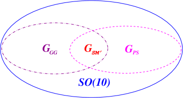
Symmetry breaking is achieved by compactification on the orbifold $T^{2}/(Z_{2}^{I}\times Z_{2}^{PS}\times Z_{2}^{GG})$. The discrete symmetries $Z_{2}$ break the extended $N=2$ supersymmetry to $N=1$, and the $SO(10)$ gauge group to the GUT subgroups (cf. Fig. (1))

$\displaystyle G_{PS}=SU(4)\times SU(2)\times SU(2)\;,\quad G_{GG}=SU(5)\times U(1)_{X}\;.$ (5)

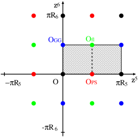
These breakings are localized at different points in the extra dimensions, $O=(0,0)$, $O_{PS}=(\pi R_{5}/2,0)$ and $O_{GG}=(0,\pi R_{6}/2)$, where

$\displaystyle P_{I}V(x,-y,-z)P_{I}^{-1}$ $\displaystyle=$ $\displaystyle\eta_{I}V(x,y,z)\;,$ (6)
$\displaystyle P_{PS}V(x,-y+{\pi R_{5}/2},-z)P_{PS}^{-1}$ $\displaystyle=$ $\displaystyle\eta_{PS}V(x,y+{\pi R_{5}/2},z)\;,$ (7)
$\displaystyle P_{GG}V(x,-y,-z+{\pi R_{6}/2})P_{GG}^{-1}$ $\displaystyle=$ $\displaystyle\eta_{GG}V(x,y,z+{\pi R_{6}/2})\;.$ (8)

Here $P_{I}=I$, the matrices $P_{PS}$ and $P_{GG}$ are given in Ref. [9], and the parities are chosen as $\eta_{I}=\eta_{PS}=\eta_{GG}=+1$. The extended supersymmetry is broken by choosing in the corresponding equations for $\Sigma$ all parities $\eta_{i}=-1$.

Refer to caption
Figure 1: The extended standard model gauge group $G_{SM^{\prime}}=SU(3)\times SU(2)\times U(1)^{2}$ as intersection of the two symmetric subgroups of $SO(10)$, $G_{GG}=SU(5)\times U(1)$ and $G_{PS}=SU(4)\times SU(2)\times SU(2)$.

There is a fourth fixpoint at $O_{fl}=(\pi R_{5}/2,\pi R_{6}/2)$, which is obtained by combining the three discrete symmetries $Z_{2}$, $Z_{2}^{PS}$ and $Z_{2}^{GG}$ defined above,

$$P_{fl}V(x,-y+{\pi R_{5}/2},-z+{\pi R_{6}/2})P_{fl}^{-1}=+V(x,y,+{\pi R_{5}/2},z+{\pi R_{6}/2})\;.$$ (9)

The unbroken subgroup at the fixpoint $O_{fl}$ is flipped $SU(5)$, i.e. $G_{fl}=SU(5)^{\prime}\times U(1)^{\prime}$. The physical region is obtained by folding the shaded regions in Fig. 2 along the dotted line and gluing the edges. The result is a ‘pillow’ with the four fixpoints as corners. The unbroken gauge group of the effective 4D theory is given by the intersection of the $SO(10)$ subgroups at the fixpoints. In this way one obtains the standard model group with an additional $U(1)$ factor,

$\displaystyle G_{SM^{\prime}}=SU(3)\times SU(2)\times U(1)_{Y}\times U(1)_{X}\;.$ (10)

The difference of baryon and lepton number is the linear combination $B-L=\sqrt{{16\over 15}}Y-\sqrt{{8\over 5}}X$. The zero modes of the vector multiplet $V$ form the gauge fields of G${}_{SM^{\prime}}$.

Refer to caption
Figure 2: $T^{2}/(Z_{2}\times Z_{2}^{PS}\times Z_{2}^{GG})$ orbifold on the $y$-$z$ plane. Four different types of fixed points, $O$, $O_{PS}$, $O_{GG}$, and $O_{FL}$, are denoted by black, red, blue, and green dots, respectively. The physical region is, for example, taken as the two-sided rectangle formed by folding the shaded region along the dotted line and then gluing together the touching edges.

The vector multiplet $V$ is a 45-plet of $SO(10)$, which has an irreducible anomaly in 6D. It is related to the irreducible anomalies of hypermultiplets in the fundamental and the spinor representations,

$$a({\bf 45})=-2a({\bf 10})\;,\quad a({\bf 16})=a({\bf 16^{*}})=-a({\bf 10})\;.$$ (11)

Hence, the cancellation of the irreducible anomalies requires two 10 hypermultiplets, $H_{1}=(H_{1},H_{1}^{c})$ and $H_{2}=(H_{2},H_{2}^{c})$, where the brackets denote the $N=1$ field content.

The parities for $H_{1}$ and $H_{2}$ may be chosen in such a way that one obtains the Higgs doublets of the MSSM as zero modes,

$\displaystyle H_{1}^{c}=H_{d}\;,\quad H_{2}=H_{u}\;.$ (12)

The D-term of the scalar potential has the flat direction $\langle H_{1}^{c}\rangle=\langle H_{2}\rangle=v$, which breaks $SU(2)\times U(1)$ to $U(1)_{em}$. The scale $v$ of electroweak symmetry breaking can be related to supersymmetry breaking, like in models of gaugino mediation.

The breaking of $B-L$ can be achieved by adding two 16 hypermultiplets, $\Phi^{c}$ and $\Phi$, with zero modes $N^{c}$, $N$. The scalar potential has the D-flat direction

$\displaystyle\langle N^{c}\rangle=\langle N\rangle=v_{N}\;,$ (13)

where $v_{N}\gg v$ can be fixed by a brane superpotential. Anomaly cancellation now requires two additional 10 hypermultiplets $H_{3}$ and $H_{4}$. The corresponding colour triplet zero modes ($D,G^{c}$) and ($D^{c},G$) aquire masses ${\cal O}(v_{N})$ from the same brane superpotential [12].

2 Flavour mixing and seesaw mechanism

So far we have constructed a gauge theory with symmetry group $SO(10)$ and $N=2$ supersymmetry in 6D, locally broken at four fixpoints, such that the effective low energy theory in 4D has $N=1$ supersymmetry and the extended SM gauge symmetry $G_{SM^{\prime}}$. In addition to the vector multiplet we have two 16 and four 10 hypermultiplets. The corresponding zero modes allow further symmetry breaking of $SU(2)\times U(1)$ and $U(1)_{B-L}$ by the ordinary Higgs mechanism.

How can matter be introduced? As our guiding principles we shall use anomaly cancellation and the embedding of quantum numbers in the adjoint representation of $E_{8}$222Such an approach has previously been pursued in the context of supersymmetric $\sigma$-models [13].. This implies that only two more 16 hypermultiplets are allowed, far too little to account for three quark-lepton generations. Hence, quarks and leptons must be brane fields. As an example, place $\psi_{1}$ at $O_{GG}$, $\psi_{2}$ at $O_{fl}$ and $\psi_{3}$ at $O_{PS}$. Here $\psi_{1}$, $\psi_{2}$ and $\psi_{3}$ correspond, up to mixings, to the first, second and third generation, respectively. We shall see that this assignment is in fact supported by fermion mass relations.

The three sequential generations are separated by distances large compared to the 6D cutoff scale $M_{*}$. Hence, they can only have diagonal Yukawa couplings with the bulk Higgs fields, since direct mixings are exponentially suppressed. On the contrary, brane fields can mix with bulk zero modes without suppression. The embedding into $E_{8}$ allows two additional 10 hypermultiplets $H_{5}$, $H_{6}$, together with two 16’s, $\phi$ and $\phi^{c}$. They lead to a partial fourth family together with an anti-family of zero modes, with the quantum numbers of lepton doublets and down-quark singlets,

$\displaystyle L=\left(\begin{array}[]{l}\nu_{4}\\ e_{4}\end{array}\right)\;,\quad L^{c}=\left(\begin{array}[]{l}\nu^{c}_{4}\\ e^{c}_{4}\end{array}\right)\;,\quad G^{c}_{5}=d^{c}_{4}\;,\quad G_{6}=d_{4}\;.$ (18)

Mixings take place only among left-handed leptons and right-handed down-quarks, which is similar to ‘lopsided’ $SU(5)$ models with $U(1)$ family symmetry [14]. This leads to a characteristic pattern of mass matrices.

Masses and mixings are determined by brane superpotentials. Allowed terms are restricted by R-invariance and an additional $U(1)_{\tilde{X}}$ symmetry. $H_{1}$, $H_{2}$, $\Phi$ and $\Phi^{c}$, which aquire a vacuum expectation value, have R-charge zero. All matter fields have R-charge one. The 16-plets $\psi_{i}$ and $\phi$ form a quartet $(\psi_{\alpha})=(\psi_{i},\phi)$, $\alpha=1\ldots 4$. The brane superpotential reads, for normalized bulk fields, up to quartic interactions (23 terms),

$\displaystyle W$ $\displaystyle=$ $\displaystyle M^{l}_{\alpha}\psi_{\alpha}\phi^{c}+{1\over 2}h^{(1)}_{\alpha\beta}\psi_{\alpha}\psi_{\beta}H_{1}+{1\over 2}h^{(2)}_{\alpha\beta}\psi_{\alpha}\psi_{\beta}H_{2}$ (19)
$\displaystyle+{1\over 2}{h^{N}_{\alpha\beta}\over M_{*}}\psi_{\alpha}\psi_{\beta}\Phi^{c}\Phi^{c}+\ldots\;.$

Here $M_{*}>1/R_{5,6}\sim\Lambda_{\rm GUT}$ is the cutoff of the 6D theory. On the different branes the Yukawa couplings $h^{(1)}$ and $h^{(2)}$ split into $h^{d},h^{e}$ and $h^{u},h^{D}$, respectively.

The breaking of $B-L$ yields masses ${\cal O}(v_{N})$ for colour triplet bulk zero modes. After electroweak symmetry breaking, $\langle H^{c}_{1}\rangle=v_{1}$, $\langle H_{2}\rangle=v_{2}$, all zero modes aquire mass terms, and one obtains

$\displaystyle W$ $\displaystyle=$ $\displaystyle d_{\alpha}m^{d}_{\alpha\beta}d^{c}_{\beta}+e^{c}_{\alpha}m^{e}_{\alpha\beta}e_{\beta}+n^{c}_{\alpha}m^{D}_{\alpha\beta}\nu_{\beta}$ (20)
$\displaystyle+u^{c}_{i}m^{u}_{ij}u_{j}+{1\over 2}n^{c}_{i}m^{N}_{ij}n^{c}_{j}\;.$

Here $m^{d}$, $m^{e}$ and $m^{D}$ are $4\times 4$ matrices, for instance,

$\displaystyle m^{e}=\left(\begin{array}[]{cccc}h^{d}_{11}v_{1}&0&0&h_{14}^{e}v_{1}\\ 0&h^{e}_{22}v_{1}&0&h_{24}^{e}v_{1}\\ 0&0&h^{d}_{33}v_{1}&h_{34}^{e}v_{1}\\ M^{l}_{1}&M^{l}_{2}&M^{l}_{3}&M^{l}_{4}\end{array}\right)\;,$ (25)

whereas $m^{u}$ and $m^{N}$ are diagonal $3\times 3$ matrices,

$\displaystyle m^{u}=\left(\begin{array}[]{ccc}h^{u}_{11}v_{2}&0&0\\ 0&h^{u}_{22}v_{2}&0\\ 0&0&h^{u}_{33}v_{2}\end{array}\right)\;,\quad m^{N}=\left(\begin{array}[]{ccc}h^{N}_{11}{v_{N}^{2}\over M_{*}}&0&0\\ 0&h^{N}_{22}{v_{N}^{2}\over M_{*}}&0\\ 0&0&h^{N}_{33}{v_{N}^{2}\over M_{*}}\end{array}\right)\;.$ (32)

Some of the mass matrix elements are equal due to GUT relations on the corresponding brane, such as $m^{e}_{11}=m^{d}_{11}$, $m^{D}_{22}=m^{u}_{22}$, whereas $m^{e}_{22}\neq m^{d}_{22}$ (flipped $SU(5)$ brane).

Assuming universal Yukawa couplings at each fixpoint, one obtains a simple pattern of quark and lepton mass matrices, significantly different from 4D $SO(10)$ models [15], which reads after a rescaling with the appropriate vauum expectation values ($\tan{\beta}=v_{2}/v_{1}\simeq 50$),

$\displaystyle{1\over\tan{\beta}}\ m^{u}\sim{v_{1}M_{*}\over v_{N}^{2}}\ m^{N}\sim\left(\begin{array}[]{ccc}\mu_{1}&0&0\\ 0&\mu_{2}&0\\ 0&0&\mu_{3}\end{array}\right)\;,$ (36)
$\displaystyle{1\over\tan{\beta}}\ m^{D}\sim m^{e}\sim m^{d}\sim\left(\begin{array}[]{cccc}\mu_{1}&0&0&\widetilde{\mu}_{1}\\ 0&\mu_{2}&0&\widetilde{\mu}_{2}\\ 0&0&\mu_{3}&\widetilde{\mu}_{3}\\ \widetilde{M}_{1}&\widetilde{M}_{2}&\widetilde{M}_{3}&\widetilde{M}_{4}\end{array}\right)\;,$ (41)

where $\mu_{i},\widetilde{\mu}_{i}={\cal O}(v_{1})$ and $\widetilde{M}_{i}={\cal O}(\Lambda_{\rm GUT})$. The quark-lepton mass spectrum requires $\mu_{i},\widetilde{\mu}_{i}$ to be hierarchical, which may be related to the different location of the three families in the extra dimension, although this is not explained by the present model. The GUT mixings $\widetilde{M}_{i}$ are assumed to be non-hierarchical.

The parameters $\mu_{1}$, $\mu_{2}$, $\mu_{3}$ are given by the up-quark masses, which also determine the heavy neutrino masses,

$\displaystyle\mu_{1}:\mu_{2}:\mu_{3}\sim m_{u}:m_{c}:m_{t}\sim M_{1}:M_{2}:M_{3}\;.$ (42)

Consider now the down-quark masses and CKM mixings for large $\tan{\beta}=v_{2}/v_{1}\simeq 50$, such that $h^{d}_{33}\simeq h^{u}_{33}$. Since the hierarchy of down-quark masses is much smaller the one of up-quarks, it must be dominated by the off-diagonal elements $\widetilde{\mu}_{i}$,

$\displaystyle\mu_{1}\ll\widetilde{\mu}_{1}\;,\quad\mu_{2}\ll\widetilde{\mu}_{2}\;,\quad\mu_{3}\sim\widetilde{\mu}_{3}\;.$ (43)

These parameters can be fixed by two masses and the Cabibbo angle,

$\displaystyle m_{b}\simeq\widetilde{\mu}_{3}\;,\quad m_{s}\simeq\widetilde{\mu}_{2}\;,\quad V_{us}=\Theta_{c}\sim{\widetilde{\mu}_{1}\over\widetilde{\mu}_{2}}\;.$ (44)

One then obtains three predictions, the other two mixing angles,

$\displaystyle V_{cb}\sim{m_{s}\over m_{b}}\simeq 2\times 10^{-2}\;,\quad V_{ub}\sim\Theta_{c}{m_{s}\over m_{b}}\simeq 4\times 10^{-3}\;,$ (45)

and the down quark mass,

$\displaystyle{m_{d}\over m_{s}}\sim\gamma\ \Theta_{c}\simeq\ 0.03\;,\quad\gamma\equiv{\mu_{2}\over\widetilde{\mu}_{2}}\sim{m_{c}m_{b}\over m_{t}m_{s}}\sim 0.1\;,$ (46)

which are consistent with data within factor of two. The charged lepton masses can also be correctly described. The unsuccessful $SU(5)$ relations $m_{s}=m_{\mu}$, $m_{d}=m_{e}$ are avoided since the second family is located at the flipped $SU(5)$ brane.

The neutrino mass matrix can now be computed based on the seesaw mechanism [5],

$\displaystyle\bar{m}_{\nu}=-\bar{m}^{D\top}{1\over m^{N}}\bar{m}^{D}\;.$ (47)

Here $\bar{m}^{D}$ is the $3\times 3$ matrix which is obtained from $m^{D}$ after integrating out the heavy fourth generation.

The structure of the charged lepton and the Dirac neutrino mass matrices is the same. Both matrices lead to large mixings between the ‘left-handed’ states. However, due to seesaw mechanism, there is a mismatch between the matrices which diagonalize the Majorana neutrino and the charged lepton mass matrices, and a large MNS mixing matrix remains. In a basis where $m^{e}$ is hierarchical, with small off-diagonal terms, the Majorana neutrino mass matrix $\bar{m}_{\nu}$ has the form

$\displaystyle\bar{m}_{\nu}\sim\left(\begin{array}[]{lll}\gamma^{2}&\gamma&\gamma\\ \gamma&1&1\\ \gamma&1&1\end{array}\right)m_{3}\;.$ (51)

This matrix is familiar from lopsided $SU(5)$ models with $U(1)$ flavour symmetry [14], and it is know to yield a successful neutrino phenomenology. Note that the small parameter is now determined by quark masses, $\gamma\sim m_{c}m_{b}/(m_{t}m_{s})$. One characteristic predictions is a large 1-3 mixing angle, $\Theta_{13}\sim\gamma\sim 0.1$. The coefficients ${\cal O}(1)$ are consistent with ‘sequential heavy neutrino dominance’ ($N_{3}$) [16], yielding large 2-3 mixing, $\sin{2\Theta_{23}}\sim 1$.

With $m_{3}\simeq\sqrt{\Delta m_{atm}^{2}}\sim m_{t}^{2}/M_{3}$ the heavy Majorana masses are $M_{3}\sim 10^{15}$ GeV, $M_{2}\sim 3\times 10^{12}$ GeV and $M_{1}\sim 10^{10}$ GeV. Decays of $N_{1}$ may be the origin of the baryon asymmetry of the universe [17]. In addition to $M_{1}$, the relevant quantities are the CP-asymmetry $\varepsilon_{1}$ and the effective neutrino mass $\widetilde{m}_{1}=(m^{D\dagger}m^{D})_{11}/M_{1}$. One easily obtains $\varepsilon_{1}\sim 0.1\;M_{1}/M_{3}\sim 10^{-6}$ and $\widetilde{m}_{1}\sim 0.2\;m_{3}$. These are the typical parameters of thermal leptogenesis [18].

One of the most puzzling questions in flavour physics is: Why are masses and mixings of quarks and neutrinos so different, and how does this happen in grand unified theories where quarks and leptons belong to the same multiplet? In the context of the discussed 6D $SO(10)$ model these questions have a simple answer:

  • The MNS mixings are large because neutrinos are mixtures of brane and bulk states, which are unrelated to quark and charged lepton masses and therefore not suppressed by small mass ratios.

  • The CKM mixings are small because left-handed down-quarks are pure brane states. The large mixings of right-handed down-quarks, together with the down-quark mass hierarchy, leads to small mixings for left-handed down-quarks.

  • Neutrinos have a small mass hierarchy because of the seesaw mechanism and the mass relations $m^{d}\sim m^{D}$, $m^{u}\sim m^{N}$; the ‘squared’ down-quark hierarchy is almost canceled by the larger up-quark hierarchy,

    $\displaystyle{m_{1}\over m_{3}}\sim\left({m_{d}\over m_{b}}\right)^{2}{m_{t}\over m_{u}}\sim 0.1\;.$ (52)

The basic mechanism determining the flavour structure is the mixing of three complete quark-lepton families, localized at three different branes, with an imcomplete family (split multiplets) originating from the bulk. This leads to welcome deviations from the familiar GUT mass relations. The mass hierarchies have a ‘geometric origin’ and are not explained by abelian or non-abelian flavour symmetries.

3 Proton decay

The 6D $SO(10)$ GUT model makes characteristic predictions for proton decay. Like in 5D orbifold GUTs, dimension-5 operators are absent [8]. The dimension-6 operators have an interesting flavour structure due to the quark-lepton ‘geography’ in the extra dimensions [19, 20].

In our 6D model the first generation is localized on the $SU(5)$ brane. This leads to the dimension-6 operators [21]

$\displaystyle{\cal L}_{\rm eff}$ $\displaystyle=$ $\displaystyle-{g^{2}\over(M_{\cal X}^{\rm eff})^{2}}\;\epsilon_{\alpha\beta\gamma}\left(e_{1}^{c}u^{c}_{1\alpha}\overline{q}_{1\beta}\overline{q}_{1\gamma}-d_{1\alpha}^{c}u^{c}_{1\beta}\overline{q}_{1\gamma}\overline{l}_{1}\right)\;,$ (53)

where

$\displaystyle\frac{1}{(M_{\cal X}^{\rm eff})^{2}}$ $\displaystyle=$ $\displaystyle 2\sum_{n,m=0}^{\infty}\frac{1}{M_{\cal X}^{2}(n,m)}$ (54)
$\displaystyle=$ $\displaystyle 2\sum_{n,m=0}^{\infty}\frac{R_{5}^{2}}{(2n+1)^{2}+\frac{R_{5}^{2}}{R_{6}^{2}}(2m)^{2}}\;$

accounts for the sum over all Kaluza-Klein modes; $R_{5}$ and $R_{6}$ are the radii of the two compact dimensions. The sum is logarithmically divergent and depends on the cutoff $M_{*}\sim 10^{17}$ GeV. In the symmetric case, $R_{5}=R_{6}=1/M_{c}$, one finds

$$\frac{1}{(M_{\cal X}^{\rm eff})^{2}}\simeq\frac{\pi}{4\,M_{c}^{2}}\left(\ln\left(\frac{M_{*}}{M_{c}}\right)+2.3\right)\;.$$ (55)
decay channel Branching Ratios [%]
6D SO(10) ${\sf SU(5)}\times{\sf U(1)}_{F}$
case I case II models A & B
$e^{+}\pi^{0}$ 75 71 54
$\mu^{+}\pi^{0}$ 4 5 < 1
$\bar{\nu}\pi^{+}$ 19 23 27
$e^{+}K^{0}$ 1 1 < 1
$\mu^{+}K^{0}$ < 1 < 1 18
$\bar{\nu}K^{+}$ < 1 < 1 < 1
$e^{+}\eta$ < 1 < 1 < 1
$\mu^{+}\eta$ < 1 < 1 < 1
Table 1: Proton decay branching ratios in a 6D $SO(10)$ model compared with 4D $SU(5)\times U(1)_{F}$ models.

The proton decay branching ratios depend on the overlap of the $SU(5)$ brane states with the mass eigenstates. Given the mass matrices of Section 2, the diagonalization can be explicitly carried out, which leads to the branching ratios listed in the table [21]. Case I and case II refer to two different sets of ${\cal O}(1)$ coefficients; the $SO(10)$ results are compared with the contribution from the dimension-6 operator in 4D $SU(5)$ models with $U(1)$ flavour symmetry.

The most striking difference is the decay channel $p\to\mu^{+}K^{0}$, which is suppressed by about two orders of magnitude in the 6D model with respect to the 4D models. In both cases the dominant decay mode is $p\to e^{+}\pi^{0}$. This is different from 5D $SU(5)$ orbifold GUTs where the dominant decay modes are $p\to K^{+}\nu$ and $p\to K^{0}\mu^{+}$ [19, 20].

Finally, a limit on the compactification scale can be derived from the decay width of the dominant channel $p\to e^{+}\pi^{0}$. One finds ($M_{*}=10^{17}$ GeV),

$$\Gamma(p\to e^{+}\pi^{0})\simeq\left(\frac{9\times 10^{15}\ {\rm GeV}}{M_{c}}\right)^{4}\left(5.3\times 10^{33}\ {\rm yrs}\right)^{-1}\;.$$ (56)

Hence, the current SuperKamiokande limit $\tau\geq 5.3\times 10^{33}$ [22] yields the lower bound on the compactification scale $M_{c}\geq M_{c}^{\rm min}\simeq 9\times 10^{15}\,{\rm GeV}$, which is very close to the 4D GUT scale $\Lambda_{\rm GUT}\simeq 2\times 10^{16}\ {\rm GeV}$ suggested by the unification of gauge couplings. The choice $M_{c}=\Lambda_{\rm GUT}$ yields the proton lifetime $\tau(p\rightarrow e^{+}\pi^{0})\simeq 1\times 10^{35}$ yrs which, remarkably, lies within the reach of the next generation of large volume detectors!

4 Towards E8 in higher dimensions

It is a remarkable group theoretical fact that the adjoint representation $\bf 45$ of $SO(10)$, together with the spinors $\bf 16$, $\bf\overline{16}$ and a $U(1)$ factor form the adjoint representation of $E_{6}$. Coset spaces of $E_{7}$ and $E_{8}$ with subgroups containing $SO(10)$ have similar properties. This raises the question whether the discussed 6D $SO(10)$ model can be understood as part of a higher-dimensional theory with gauge group $E_{8}$, as it emerges in string theory [23].

Consider the chain of $E_{8}$ subgroups

$$E_{8}\supset SO(16)\supset SO(10)\times SO(6)\supset\ldots,$$ (57)

and the corresponding decomposition of the adjoint representation,

$\displaystyle{\bf 248}$ $\displaystyle=$ $\displaystyle{\bf 120}+{\bf 128}$ (58)
$\displaystyle=$ $\displaystyle{\bf(45,1)}+{\bf(1,15)}+{\bf(10,6)}+{\bf(16,4)}+{\bf(\overline{16},\overline{4})}\;.$

As discussed in Section 2, the 6D $SO(10)$ model has $N=2$ supersymmetry. The $\bf 45$ vector multiplet of $SO(10)$, and the six $\bf 10$ and four $\bf 16$ hypermultiplets represent the maximal number of fields from the adjoint of $E_{8}$ for which the irreducible 6D anomalies cancel. For this particular set of fields, also the reducible 6D anomalies cancel [11].

Orbifold GUT models of the type discussed in this talk can occur as intermediate step in an orbifold compactification of the heterotic string [24, 25]. The model of Ref. [24]
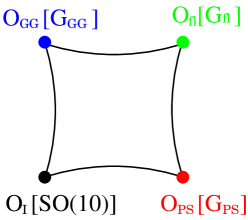
Refer to caption
Figure 3: The three $SO(10)$ subgroups at the corresponding fixpoints of the orbifold $T^{2}/(Z_{2}^{I}\times Z_{2}^{PS}\times Z_{2}^{GG})$. At each of these fixpoints one quark-lepton family is localized.

indeed contains a 6D $SO(10)$ GUT with the set of bulk fields described above. At the orbifold fixpoints states from the twisted sector of the string are localized, as illustrated in Fig. 3 for the considered orbifold GUT.

Orbifold GUTs have many phenomenologically attractive features. In particular split multiplets successfully explain the doublet-doublet splitting of Higgs fields. Their mixing with brane fields also leads to flavour physics with unexpected features and the needed deviations from the simplest GUT mass relations.

A successful ultraviolet completion in compactifications of the heterotic string will allow to address many questions which go beyond orbifold GUTs. These include quantum numbers and localization of brane fields, which are related to twisted sectors of the string, and the unification with gravity.

I would like to thank T. Asaka, L. Covi, D. Emmanuel-Costa and S. Wiesenfeldt for a fruitful collaboration, A. Hebecker for comments on the manuscript and the organizers of the seesaw symposium at KEK, especially K. Nakamura, for arranging an enjoyable and stimulating meeting.

References

  • [1] H. Georgi, S. L. Glashow, Phys. Rev. Lett. 32 (1974) 438.
  • [2] J. C. Pati, A. Salam, Phys. Rev. D 10 (1974) 275.
  • [3] H. Georgi, Particles and Fields 1974, ed. C. E. Carlson (AIP, NY, 1975) p. 575;
    H. Fritzsch, P. Minkowski, Ann. of Phys. 93 (1975) 193.
  • [4] S. M. Barr, Phys. Lett. B 112 (1982) 219;
    J. P. Derendinger, J. E. Kim, D. V. Nanopoulos, Phys. Lett. B 139 (1984) 170.
  • [5] T. Yanagida, in Workshop on unified Theories, KEK report 79-18 (1979) p. 95;
    M. Gell-Mann, P. Ramond, R. Slansky, in Supergravity (North Holland, Amsterdam, 1979) eds. P. van Nieuwenhuizen, D. Freedman, p. 315
  • [6] L. J. Dixon, J. A. Harvey, C. Vafa, E. Witten, Nucl. Phys. B 261 (1985) 678; ibid. Nucl. Phys. B 274 (1986) 285.
  • [7] L. E. Ibáñez, H. P. Nilles, F. Quevedo, Phys. Lett. B 187 (1987) 25;
    L. E. Ibáñez, J. E. Kim, H. P. Nilles, F. Quevedo, Phys. Lett. B 191 (1987) 282.
  • [8] Y. Kawamura, Progr. Theor. Phys. 103 (2000) 613; ibid. 105 (2001) 999;
    G. Altarelli, F. Feruglio, Phys. Lett. B 511 (2001) 257;
    L. J. Hall, Y. Nomura, Phys. Rev. D 64 (2001) 055003;
    A. Hebecker, J. March-Russell, Nucl. Phys. B 613 (2001) 3.
  • [9] T. Asaka, W. Buchmüller, L. Covi, Phys. Lett. B 523 (2001) 199;
    L. J. Hall, Y. Nomura, T. Okui, D. R. Smith, Phys. Rev. D 65 (2002) 035008.
  • [10] R. Dermisek, A. Mafi, Phys. Rev. D 65 (2002) 055002;
    H. D. Kim, S. Raby, JHEP 0301 (2003) 056.
  • [11] T. Asaka, W. Buchmüller, L. Covi, Phys. Lett. B 563 (2003) 209.
  • [12] T. Asaka, W. Buchmüller, L. Covi, Phys. Lett. B 540 (2002) 295.
  • [13] W. Buchmüller, S. T. Love, R. D. Peccei, T. Yanagida, Phys. Lett. B 115 (1982) 233;
    C. L. Ong, Phys. Rev. D 27 (1983) 3044; ibid. Phys. Rev. D 31 (1985) 3271;
    S. Irié and Y. Yasui, Z. Phys. C29 (1985) 123;
    W. Buchmüller, O. Napoly, Phys. Lett. B 163 (1985) 161;
    K. Itoh, T. Kugo, H. Kunitomo, Progr. Theor. Phys. 75 (1986) 386.
  • [14] J. Sato, T. Yanagida, Phys. Lett. B 430 (1998) 127;
    N. Irges, S. Lavignac, P. Ramond, Phys. Rev. D 58 (1998) ;
    G. Altarelli, F. Feruglio and I. Masina, hep-ph/0405048.
  • [15] C. H. Albright, Int. J. Mod. Phys. A 18 (2003) 3947.
  • [16] S. F. King, Nucl. Phys. B 576 (2000) 85.
  • [17] M. Fukugita, T. Yanagida, Phys. Lett. B 174 (1986) 45.
  • [18] W. Buchmüller, M. Plümacher, Phys. Lett. B 389 (1996) 73;
    W. Buchmüller, T. Yanagida, Phys. Lett. B 445 (1999) 399.
  • [19] Y. Nomura, Phys. Rev. D 65 (2002) 085036.
  • [20] A. Hebecker and J. March-Russell, Phys. Lett. B 539 (2002) 119.
  • [21] W. Buchmüller, L. Covi, D. Emmanuel-Costa, S. Wiesenfeldt, hep-ph/0407070.
  • [22] Y. Suzuki et al. [TITAND Working Group Collaboration], arXiv:hep-ex/0110005.
  • [23] M. B. Green, J. H. Schwarz, E. Witten, Superstring Theory, Cambridge Univ. Press, Cambridge, 1987.
  • [24] T. Kobayashi, S. Raby, R.-J. Zhang, hep-ph/0403065.
  • [25] S. Förste, H. P. Nilles, P. Vaudrevange, A. Wingerter, hep-th/0406208.