Twisted Split Fermions

Abstract

The observed flavor structure of the standard model arises naturally in “split fermion” models which localize fermions at different places in an extra dimension. It has, until now, been assumed that the bulk masses for such fermions can be chosen to be flavor diagonal simultaneously at every point in the extra dimension, with all the flavor violation coming from the Yukawa couplings to the Higgs. We consider the more natural possibility in which the bulk masses cannot be simultaneously diagonalized, that is, that they are twisted in flavor space. We show that, in general, this does not disturb the natural generation of hierarchies in the flavor parameters. Moreover, it is conceivable that all the flavor mixing and CP-violation in the standard model may come only from twisting, with the five-dimensional Yukawa couplings taken to be universal.

I Introduction

One of the motivations to extend the Standard Model (SM) is to explain the fermion flavor structures. It is likely that there is a more fundamental theory that produces the observed masses and mixing angles in a natural way, namely, without small dimensionless parameters. One such framework uses split fermions to generate the small numbers AS . The basic idea is to localize the SM fermion fields at different locations in compact extra dimensions. Then, the four dimensional (4D) Yukawa couplings between left handed and right handed 4D fermion fields are exponentially suppressed by the overlap of the corresponding zero mode wavefunctions. In general, such a split fermions setup induces small and hierarchical 4D Yukawa couplings without imposing any extra symmetries. In addition, one can account for proton stability by separating quarks and leptons in the extra dimension. Specific realizations, phenomenological implications and experimental signatures of the split fermions framework can be found in AS ; MS ; GGH ; KT ; PDG ; ASmodels ; GT ; Mats ; Branco ; GP ; GrPe ; GaussLocH ; LocH ; NP ; AGS .

Fermion localization works as follows AS ; MS ; PDG . Consider, for simplicity, a model with one infinite extra dimension. (For the more realistic case of a finite extra dimension see, for example, GGH ; KT ; GrPe .) The model contains one bulk scalar, the localizer, which is assumed to get a vacuum expectation value (vev) which depends on the extra dimension coordinate, $z$. Thus, the five dimensional (5D) Dirac spinors have two mass terms: a $z$-independent bare mass and a $z$-dependent mass term due to the couplings to the localizer. For $\Psi_{i}$, a generic Dirac field (with $i=1,2,3$ as the generation index) and $\Phi(z)$, the localizer vev, these mass terms read

$${\cal L}=\bar{\Psi}^{i}\tilde{M}_{ij}(z)\Psi^{j},\qquad\tilde{M}_{ij}(z)\equiv m_{ij}+\lambda_{ij}\Phi(z)\,,$$ (1)

where $m_{ij}$ and $\lambda_{ij}$ are $z$-independent Hermitian matrices.

In the past is was always assumed that $m_{ij}$ and $\lambda_{ij}$ can be diagonalized simultaneously. In that case the problem of obtaining the 4D observables is significantly simpler. We can carry out the Kaluza-Klein (KK) decomposition of the 5D fields in the basis in which the mass matrix is diagonal. Each zero mode, which is interpreted as the corresponding SM chiral fermion field, then has a wavefunction in the extra dimension $f_{i}(z)$. These wavefunctions must satisfy the condition derived from the 5D Dirac equation:

$$\left[\partial_{z}-\tilde{M}_{i}(z)\right]f_{i}(z)=0,\qquad\tilde{M}_{i}=[m_{ii}+\lambda_{ii}\Phi(z)]\,,$$ (2)

where $\partial_{z}\equiv\partial/\partial z$. The solution is

$${f_{i}}(z)=f_{i}(0)\exp\left[\int_{0}^{z}\tilde{M}_{i}(z^{\prime})dz^{\prime}\right]\,,$$ (3)

where $f_{i}(0)$ is an arbitrary vector that specifies the values of the solutions at $z=0$. For example, in the case where the localizer vev is linear, the zero mode wavefunctions are Gaussians AS ; MS . These Gaussians peak at the points where $\tilde{M}_{i}(z)=0$. The fact that the wavefunctions which correspond to different generations are localized at different points leads to the required small overlaps.

In this work we relax the assumption that the parameters in the Lagrangian should be aligned in flavor space, that is, we assume that $m_{ij}$ and $\lambda_{ij}$ cannot be diagonalized simultaneously. We call the unaligned case “twisted”, and the aligned case “untwisted”. We will focus on answering the following two questions related to the attractive features of the split fermions framework:

• In the presence of twisting, can one naturally suppress operators which involve fields in different representations? This is required to account for the proton longevity.

• In the presence of twisting, are the hierarchies between operators which involve fields from the same representation still natural? This is required to account for the flavor puzzle.

As we demonstrate below the answer to both of the above questions is positive: The presence of twisting does not spoil the basic appealing features of the split fermions framework.

Once we understand how twisting affects hierarchies, we can ask whether twisting may also be useful for model building. Again the answer is positive. One example is related to the fact that twisting induces new CP violating sources. This was used in NP to construct a new type of leptogenesis model. Below we demonstrate how the standard model flavor mixing and CP violation may arise purely from twisting. Another possible application is related to a solution of the strong CP problem, which will be discussed in a separate work.

II The Twist - Basic formalism

We consider the most general Lagrangian of Eq. (1). We would like to find the profile of the zero modes and calculate the 4D observables in terms of the 5D Lagrangian parameters. The answer is nontrivial because the effective mass matrix of the fermions $\tilde{M}_{ij}(z)$ is a $z$-dependent Hermitian matrix. There is no global $SU(3)$ flavor transformation which brings $\tilde{M}_{ij}(z)$ to a diagonal form simultaneously at every $z$. $\tilde{M}_{ij}(z)$ can be diagonalized by a $z$-dependent special unitary matrix $U(z)$, however this does not leave the 5D kinetic terms invariant. This is to be compared to the untwisted case where $U$ is $z$-independent. Formally we can introduce a local measure of the twist by

$$R_{ij}(z)=\left[\tilde{M}_{ik}(z),{d\over dz}\,\tilde{M}_{kj}(z)\right].$$ (4)

When $R_{ij}(z)$ is non-zero, a twist is present in that region. Only when $R_{ij}(z)=0$ for all values of $z$ does the general (twisted) case reduce to the flavor-aligned (untwisted) case.

In the general twisted case the KK decomposition for a vector (in flavor space) fermion field is given by

$$\Psi_{i}(x_{\mu},z)=\sum_{n,\alpha}(f_{L}^{n})_{i\alpha}(z)P_{L}\psi^{n}_{\alpha}(x_{\mu})+\sum_{n,\alpha}(f_{R}^{n})_{i\alpha}(z)P_{R}\psi^{n}_{\alpha}(x_{\mu})\,,$$ (5)

where $x_{\mu}$ are the known four dimensions, $(f_{L}^{n})_{i\alpha}$ and $(f_{R}^{n})_{i\alpha}$ are $z$-dependent wavefunctions, and $P_{L}\,(P_{R})$ is the left (right) handed chirality projection operator. Our notation is such that 5D (4D) fields are denoted by capital (lowercase) letters. We can think about the Latin (Greek) indices as labeling the flavor space in 5D (4D). Note that the 5D wavefunctions, $f_{R}^{n}$ and $f_{L}^{n}$, are generic $z$-dependent matrices in flavor space, as compared to the untwisted case AS , where they were diagonal and hence simply functions.

We are interested in the zero modes since they correspond to the SM fermions. Consider, for example, the wavefunctions of the left handed zero modes, $f_{j\alpha}(z)$. These must satisfy the condition derived from the 5D Dirac equation:

$$\left[\delta_{ij}\partial_{z}-\tilde{M}_{ij}(z)\right]f_{j\alpha}(z)=0\,,$$ (6)

where $i,j=1\ldots 3$ stand for the three components of a single wave function, while $\alpha=1\ldots 3$ labels the three different solutions to this equation and thus corresponds to the SM flavor indices. The solution may be written formally in a straightforward way:

$$f_{i\alpha}(z)=P\exp\left[\int_{0}^{z}\tilde{M}_{ij}(z^{\prime})dz^{\prime}\right]\times f_{j\alpha}(0)\,,$$ (7)

where $P$ stands for the path ordered product and $f_{j\alpha}(0)$ is an arbitrary $3\times 3$ matrix that specifies the values of the different solutions at $z=0$. In principle, we can choose $f_{j\alpha}(0)$ such that the three vectors $f_{i1}$, $f_{i2}$ and $f_{i3}$ constitute a set of orthonormal eigenvectors:

$$\int dz\,f^{*}_{i\alpha}(z)\,f_{i\beta}(z)=\delta_{\alpha\beta}\,.$$ (8)

In practice, we can just choose the vectors to be linearly independent and then get an orthonormal set by applying the Gram-Schmidt procedure.

The nontrivial difference between the twisted (7) and untwisted (3) case is that with twisting one cannot factorize the solution of the zero modes into a form of flavor-space times $z$-space. At each point, each solution is a vector in flavor space, but the twisting forces it to rotate (twist) as it moves along the extra-dimension. This follows directly from the fact that with twisting the matrix $\tilde{M}_{ij}$ cannot be diagonalized simultaneously at all $z$.

Unfortunately, in the most general twisted case, equation (7) is not very instructive (although it can be used for numerical computations). In certain cases even with twisting we can find explicit solutions. For example, in two generations, the two coupled first-order differential equations (6) can be combined into a single second order equation. Then, if $\tilde{M}$ has a simple enough form, we may be able to find solutions. For example, if $\tilde{M}$ depends linearly on $z$, the solutions are Kummer functions (see Appendix A). In three generations the composite equation is third order and is in general unsolvable, even with a linear $\tilde{M}$.

In order to obtain the 4D observables we start from the 5D couplings of the fermions to the SM Higgs field. Consider for example the couplings of the quarks doublets, $Q_{i}$, to the down type quark singlets, $D_{j}$,

$$S=\int d^{5}xY^{d}_{ij}H\bar{Q}_{i}D_{j}\,,$$ (9)

where $H$ is the SM Higgs field and the Dirac structure is suppressed. The 5D Yukawa couplings, $Y^{d}_{ij}$, are assumed to be arbitrary parameters without any specific flavor structure. Performing the KK reduction, assuming that the profile of the Higgs vev is flat, and keeping only the zero modes, we obtain the standard 4D action

$$S=\int d^{4}x\,y^{d}_{\alpha\beta}\,h\,\bar{q}_{\alpha}\,d_{\beta}\,.$$ (10)

The dimensionless 4D Yukawa couplings are given by

$$y^{d}_{\alpha\beta}=\int dzY^{d}_{ij}\,f^{q*}_{i\alpha}(z)\,f^{d}_{j\beta}(z)\,,$$ (11)

where $f^{q}$ ($f^{d}$) is the wavefunction of the left (right) handed quark doublet (down type singlet) and the sum over $i$ and $j$ is implicit.

For simplicity, here and in it what follows, we work with rescaled parameters. That is, we scale constants and wavefunctions to the appropriate power of the fundamental scale to make them dimensionless.

III General properties of the zero modes

In the following two sections we demonstrate that twisting does not destroy the essential appealing features of the split fermions framework, namely, localization and separation of the fermion zero modes.

First, consider localization. We confine our discussion to the case were the eigenvalues of $\tilde{M}_{ij}(z)$ are monotonically decreasing functions of $z$ (as is the case in the models of AS ). In the untwisted case the peaks of the zero modes are located at the points where one of the flavors has a zero bulk mass. This implies that we can separate fermions in different representations, for example quarks and leptons, to forbid proton decay. In this section we show that a similar localization holds in the twisted case as well.

To see this, we show that since the eigenvalues of $\tilde{M}_{ij}(z)$ are monotonic functions of $z$, we can define a “localization region”. We define this region as the region between the two points $z_{a}$ and $z_{b}$ such that for $z<z_{a}$ ($z>z_{b}$) all the eigenvalues are positive (negative). The magnitude of each of the zero modes, $|f_{\alpha}|^{2}\equiv\sum_{i}f^{*}_{i\alpha}f_{i\alpha}$, decays outside the localization region as is shown below.

It is sufficient to study the norm of the wavefunction because the overlap between the norms provides an upper bound on the overlap between the actual wavefunctions,

$$\int dzf_{i\alpha}^{q*}(z)f_{j\beta}^{u}(z)\leq\int dz|f_{\alpha}^{q}(z)||f_{\beta}^{u}(z)|,$$ (12)

which serves as a bound on the effective 4D couplings. Using eq. (6) we obtain

$$\partial_{5}|f_{\alpha}(z)|^{2}=2\sum_{k}m_{k}(z)|f_{k\alpha}(z)|^{2}.$$ (13)

where there is no sum on the index $\alpha$ and $m_{k}(z)$ are the eigenvalues of $\tilde{M}_{ij}(z)$. We denote by $m_{\max}(z)$ [$m_{\min}(z)$] the maximal [minimal] eigenvalue of $\tilde{M}$ at $z$. Then, we can place bounds on the right hand side of equation (13)

$$m_{\min}|f_{\alpha}(z)|^{2}\leq\sum_{i}m_{i}(z)|f_{i\alpha}(z)|^{2}\leq m_{\max}|f_{\alpha}(z)|^{2}\,.$$ (14)

We see that the norms of the zero modes fall at large positive and negative values. In particular,

$$|f_{\alpha}(z)|^{2}\leq\exp\left[2{\int_{z_{b}}^{z}dz^{\prime}m_{\max}(z^{\prime})}\right]|f_{\alpha}(z_{b})|^{2}\qquad{\rm for}~{}z>z_{b}.$$ (15)

Note that $m_{\max}<0$ over all of the integration range. A similar bound may be placed in the $z<z_{a}$ region

$$|f_{\alpha}(z)|^{2}\leq\exp\left[-2\int_{z}^{z_{a}}dz^{\prime}m_{\min}(z^{\prime})\right]|f_{\alpha}(z_{a})|^{2}\qquad{\rm for}~{}z<z_{a},$$ (16)

where $m_{\min}>0$ all over the integration range. We see that the norm of the wave function indeed decays outside the localization region.

The above arguments hold separately for each SM representation. Thus, different representations can be separated if their localization regions do not overlap. In models where the localizer vev is linear, like that of AS , $m_{\max}$ and $m_{\min}$ are roughly linear far away from the localization region. In that case the bounds in equations (15) and (16) imply that far from the localization region the norms of the zero modes are suppressed exponentially (as Gaussians). The generalization to the more realistic models in which a stable scalar configuration is not a monotonic function of $z$ is straightforward. In these cases one can divide the extra dimension into regions where the scalar is monotonic and apply the above analysis for each of the regions separately. Thus we have answered question (i) from the introduction: fermions in different representations can be naturally separated.

IV The Adiabatic Approximation

Though we have shown that exponentially small overlaps are easily achieved between different representations, in order to solve the flavor puzzle hierarchies within a representation are required. To see whether this is the case in our framework one needs a better handle on the profiles of fermions zero modes. As we already mentioned, the general solution to the zero mode wavefunction equation is not very useful in this respect. Here we show that in many cases one can make an approximation in which the governing physics is clear.

The zero mode equation (6) bears resemblance to the time dependent Schrödinger equation, $i\partial_{t}|\psi\rangle=H|\psi\rangle$, with $it$ replaced by $z$. The $z$ dependent $\tilde{M}$ corresponds to a time varying Hamiltonian. One of the useful approximation methods for solving a time varying Hamiltonian in quantum mechanics is the adiabatic approximation messiah where the wavefunction is assumed to be an instantaneous energy eigenstate at all times.

It is useful to make a similar approximation in our case. The assumption we make is that the independent solutions of eq. (6) are each governed by a single eigenvalue of the mass matrix at each point in the extra dimension. We thus expect each solution to be aligned with one of the eigenvectors of $\tilde{M}(z)$ at each point.

We begin by writing an ansatz for the solution to the equation which satisfies the guideline mentioned above. The ansatz for the left handed zero mode profile is

$$f^{\mathrm{ad}}_{i\alpha}\left(z\right)={1\over N}\,\exp\left[\int_{0}^{z}dz^{\prime}\,m_{\alpha}\left(z^{\prime}\right)\right]V_{i\alpha}\left(z\right)\,,$$ (17)

where $V_{i\alpha}(z)$ are the $z$ dependent normalized eigenvectors of the twisted bulk mass matrix

$$\tilde{M}_{ij}(z)V_{j\alpha}\left(z\right)=m_{\alpha}(z)V_{i\alpha}(z)\qquad\mbox{with}\qquad V_{i\alpha}^{*}V_{i\beta}=\delta_{\alpha\beta}\,.$$ (18)

Within this approximation each zero mode is localized around the zero of a single ($z$ dependent) eigenvalue of the mass matrix. The adiabatic ansatz is thus a straightforward generalization of the untwisted solution. In both cases the wavefunction of each profile is governed by a single function which is an eigenvalue of the bulk mass matrix and therefore in both cases the wavefunctions are localized. In the adiabatic limit the only added feature introduced with twisting is that the wavefunction points in different directions in flavor space for various values of $z$.

To what extent is the adiabatic approximation valid in generic models? The standard condition in quantum mechanics literature is that the approximation holds so long as the quantity

$$\frac{\langle V_{1}|\partial_{z}\tilde{M}|V_{2}\rangle}{(m_{1}-m_{2})^{2}},$$ (19)

is small throughout the evolution of the system messiah . Our case however, is somewhat more subtle due to the fact that the evolution of the wavefunctions with ‘time’ is not unitary. The rate at which the true solution deviates from the adiabatic one at a certain point is indeed proportional to the quantity in eq. (19) but is also depends on the values of the wavefunctions at that point.

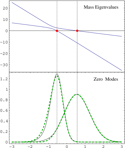
Figure 1: The two solid blue lines in the upper figure are the eigenvalues of the mass matrix $\tilde{M}(z)$ given in eq. (20). The localization region defined in the previous section lies between the two vertical dotted lines. The exact solution to the norm of the wavefunctions is in the lower figure in solid lines while the adiabatic approximation is in thick dashed green curves. Note that the departure of the adiabatic solution from the exact one occurs where the two eigenvalues approach one another.

We did not try here to fully formulate and derive the necessary conditions for the validity of the above approximation. One can, however, get good intuition by numerically comparing it with the exact solution, eq. (7). This allows us to learn about the accuracy of the adiabatic approximation. As an example consider the following mass matrix for the two generation case

$$\tilde{M}(z)=\pmatrix{-2z+1&1\cr 1&-5z-10}\,,$$ (20)

where we work with rescaled parameters such that $z$ and $\tilde{M}$ are dimensionless. In the upper part of figure 1 we plot the two eigenvalues of the mass matrix and in the lower part of the figure 1 we plot the norm of adiabatic solution that is induced by the eigenvalues (green dashed curves). For comparison the adiabatic curves are plotted on top of the exact solution (black solid lines).

We see that in the case presented in figure 1 the adiabatic approximation is very good. It noticeably deviates from the exact solution only in the region where the two eigenvalues approach one another as one would expect from eq. (19). This departure only occurs once both profiles have decayed (or have started to do so). Consequently, physical quantities are hardly affected and the approximation holds to a very good accuracy.

We expect this behavior to be generic in models that have well localized and separated wavefunctions. This is because separation implies that at the points $z_{i}$, where any of the mass eigenvalues vanishes, the mass differences are large. Thus, non-adiabatic contributions are supressed near $z_{i}$. If the eigenvalues are changing smoothly the non-adiabaticity generically occurs well outside the localization region. We have indeed observed that increasing the separation (and hierarchy) between flavors improves the approximation. We have checked numerically several cases that lead to hierarchical Yukawa matrices and found that the adiabatic approximation works very well in these cases.

V Hierarchies and mixing from twisting

So far we have shown that even with twisting, localization and separation within a representation naturally occur. In this section we discuss twisting as the only source of flavor mixing and CP violation. We consider below the following two questions:

• Can all the flavor mixing and CP violation come from twisting? That is, can we take the 5D Yukawa matrices to be universal, so that all of the SM flavor structure comes from twisting?

• Can the above scenario be realized naturally?

We show that the answer to the above two questions is positive. We first demonstrate numerically that twisting can serve as the only source of flavor mixing. Then we support this observation, for more generic cases, using the adiabatic approximation. Finally, we present a toy model in which this situation occurs naturally.

Let us begin with the numerical example. We denote the mass matrices as

$$\tilde{M}_{ij}^{r}\left(z\right)=m_{ij}^{r}-\eta_{ij}^{r}z\,.$$ (21)

with $r=Q,U,D$. We assume that the 5D Yukawa couplings are proportional to the unit matrix. Then, the Lagrangian of the model is given schematically by

$${\cal L}=Y^{U}\delta_{ij}H\bar{Q}_{i}\,U_{j}+Y^{D}\delta_{ij}H\bar{Q}_{i}\,D_{j}+\tilde{M}_{ij}^{Q}\bar{Q}_{i}Q_{j}+\tilde{M}_{ij}^{U}\bar{U}_{i}U_{j}+\tilde{M}_{ij}^{D}\bar{D}_{i}D_{j}\,.$$ (22)

When $m^{r}_{ij}$ and $\eta^{r}_{ij}$ can be diagonalized simultaneously this model is untwisted. In the most generic case, however, when no symmetry is imposed, the mass matrix is expected to be twisted. For our explicit example we choose the following parameters for the bulk masses

$$\tilde{M}^{Q}(z) = \pmatrix{3.4\,z-4&2.3\cr 2.3&2.6\,z-6}\,,$$

$$\tilde{M}^{D}(z) = \pmatrix{4.1\,z+1&1\cr 1&3.1\,z-3}\,,$$

$$\tilde{M}^{U}(z) = \pmatrix{4.5\,z+4&1\cr 1&2.9\,z+2}\,,$$ (23)

where we work with rescaled parameters such that $z$ and $\tilde{M}^{r}$ are dimensionless. We obtain hierarchical fermion masses

$${m_{d}\over m_{s}}=2.1\times 10^{-1},\qquad{m_{u}\over m_{c}}=8.0\times 10^{-3},$$ (24)

and finite mixing

$$\sin\theta_{C}=0.19.$$ (25)

Note that this is only an example. We did not try to search for a mass matrix which precisely generates the observed 4D flavor parameters. We use this example only to demonstrate the fact that 4D flavor mixing and hierarchical masses can originate only from the twisting.

While we gave an explicit example only for one simple case, the conclusion holds much more generally. To see this, we use the adiabatic approximation. Using Eqs. (11) and (17) we see that

$$y^{d}_{\alpha\beta}\approx{1\over N_{Q}N_{D}}\int dz\exp\left[\int_{0}^{z}dz^{\prime}\,m^{Q}_{\alpha}\left(z^{\prime}\right)\right]\exp\left[\int_{0}^{z}dz^{\prime}\,m^{D}_{\beta}\left(z^{\prime}\right)\right]V_{i\alpha}^{Q}\left(z\right)V_{i\beta}^{D*}\left(z\right)\,.$$ (26)

The exponential factors in (26) teach us that we expect a hierarchical structure for the 4D Yukawa couplings. In addition, for the realistic case of three generations, the product ${V^{Q}_{i\alpha}}V^{D*}_{i\beta}$ is just a product of two $SU(3)$ matrices. This shows that flavor mixing is induced. Furthermore, these $SU(3)$ matrices generically contain ${\cal O}$(1) phases. Thus, $\delta_{\rm CKM}$, the CP violating phase in the 4D CKM matrix, is expected to be of order unity as observed.

The above numerical study exemplifies the possibility that all of the SM flavor conversion is achieved due to the twist in the bulk, and not due to the 5D Yukawa couplings. Below we construct a toy model which naturally realizes this idea. Consider a model for quarks with a non-Abelian horizontal flavor symmetry $SU(3)_{F}$ on a 5D orbifold $M_{4}\times S_{1}/Z_{2}$. The fermions, $Q^{i},U^{i},D^{i}$ are fundamentals of the flavor group where all other SM fields are singlets. The Higgs field, the left handed component of $Q^{i}$ and the right handed component of $D^{i}$ and $U^{i}$ are even under the $Z_{2}$ orbifold symmetry, and all the other fields are odd. Because of the orbifold symmetry, a bulk mass for the fermions is forbidden. But an effective mass can be generated from the vev of $Z_{2}$ odd bulk scalars that are SM singlets. For our example, we include an adjoint (octet) $\Phi_{ij}$ and a singlet $\phi$ of $SU(3)_{F}$. The Yukawa couplings to the Higgs, on the other hand, are allowed and are proportional to unit matrices due to the flavor symmetry.

Generically, there is a potential for the scalars in the bulk. This potential naively generates an untwisted scalar vev since varying vevs are usually not the lowest energy configuration. Thus, we also include boundary terms that change this naive expectation. When the symmetry is explicitly broken on the boundaries, the competition between the bulk and boundary terms can force the vev of $\Phi$ to be twisted.

To be explicit, consider the case in which the boundaries preserve only an $SU(2)$ subgroup of the bulk $SU(3)_{F}$. Under this $SU(2)$, $\Phi_{ij}$ decomposes into a scalar $\Phi\equiv\Phi_{33}$, a fundamental $\Phi_{l}=\left(\Phi_{13},\Phi_{23}\right)$, an antifundamental $\Phi_{l}^{*}$, and an adjoint $\Phi_{lm}$ with $l,m=1,2$. For each of the above fields we can write a boundary term

$$-{\cal L}^{\rm brane}_{\Phi}=\sum_{B=0,\pi R}\left[a_{B}^{2}\left(\partial_{z}\Phi\right)^{2}+b_{B}^{2}\left(\partial_{z}\Phi_{l}\right)^{2}+c_{B}^{2}\left(\partial_{z}\Phi_{lm}\right)^{2}\right]+\ldots$$ (27)

where higher order (stabilizing) terms are omitted for simplicity. The parameters $a_{0,\pi R}$, $b_{0,\pi R}$ and $c_{0,\pi R}$ are real and generically different on the two different branes. The terms above cause non-zero vevs to be developed for the derivative of $\Phi,\Phi_{1}$ and $\Phi_{lm}\,$ at $z=0$

$$\langle\partial_{z}\Phi\rangle|_{0}={\cal O}(1)\,,\ \ \ \langle\partial_{z}\Phi_{l}\rangle|_{0}=\pmatrix{0\cr{\cal O}(1)}\,,\ \ \ \langle\partial_{z}\Phi_{lm}\rangle|_{0}=H_{lm}\,,$$ (28)

where $H_{lm}$ is an order one Hermitian matrix and we used an $SU(2)$ transformation to bring the vev of $\partial_{z}\Phi_{l}$ to its special form. Similarly, at $z=\pi R$ the derivatives get non-vanishing vevs, which are generically different from those at $z=0$. Consequently, the mass matrix at both boundaries are not aligned and a twist is generated in the bulk.

We assume that $v^{2}_{F}/\Lambda^{2}\ll 1$ where $v_{F}$ is the typical vev of the bulk scalars and $\Lambda$ is the effective cutoff of the 5D theory. Then, to leading order in $v^{2}_{F}/\Lambda^{2}$, the 5D Lagrangian is given by eq. (22) with

$$\tilde{M}_{ij}^{r}=c_{1}^{r}\langle\Phi_{ij}\rangle+c_{2}^{r}\langle\phi\rangle\,,$$ (29)

where $c_{1}^{r}$ and $c_{2}^{r}$ are unknown constants. We see that the 5D Yukawa couplings are proportional to the unit matrix and that $\tilde{M}_{ij}^{r}$ cannot be globally diagonalized at each $z$ because it is twisted. Due to the fact that the bulk scalars are odd under the $Z_{2}$ orbifold symmetry the correction to the universal Yukawa matrices is suppressed by ${\cal O}(v^{2}_{F}/\Lambda^{2})$. There are additional higher dimension brane Yukawa terms which are volume suppressed and are therefore negligible. We conclude that in this toy model the 4D flavor violation is, to leading order, only due to twisting.

VI Discussions and conclusions

We found that in many ways neglecting the twist is a simplifying assumption. Twisting does not change the fact that split fermions generically produce hierarchical Yukawa couplings. At first neglecting the twist seems unjustified: it changes the symmetry breaking pattern of the theory. For example, suppose there is a single fermion representation in the bulk, with 3 flavors. When $\tilde{M}(z)\propto{\mathbf{1}}_{3}$ there is an enhanced $U(3)$ flavor symmetry in the theory. Including a diagonal $\tilde{M}(z)$ breaks the $U(3)$ symmetry down to $U(1)^{3}$. Including a generic twisted $\tilde{M}(z)$ breaks it further to $U(1)$ NP . In untwisted models this last step occurs only due to the standard model Yukawa interactions.

In the untwisted case the fact that we get hierarchical Yukawa couplings and small mixing can be understood from symmetry considerations as follows. The $U(1)^{3}\to U(1)$ breaking is due to non-diagonal 5D Yukawa couplings, which connect fields of different SM representations, and therefore, the last stage of symmetry breaking occurs between objects that are separated in the extra dimension. Thus, the 4D Yukawa couplings are small since they are suppressed by the small overlap of the separated zero modes. That is, the $U(1)^{3}$ remains as an approximate symmetry, and it is restored once the zero mode wavefunctions are far away from each other.

In the twisted case the fact that an approximate $U(1)^{3}$ symmetry is obtained in the low energy effective theory is less obvious. Nevertheless, we claim that this remain the case due to the same reason, namely, symmetry breaking occurs between objects that are separated in the extra dimension. In other words, even with the twist, we have shown that the zero modes are localized and separated. This implies that the 4D Yukawa couplings are small since they are proportional to the small overlap of the different zero modes. Just like in the untwisted case, when the separation is very large, the $U(1)^{3}$ symmetry is restored. Thus, the effect of the twist is only to add new sources of flavor mixing and CP violation.

In conclusion, the main result from our study is that the twist does not affect the general appealing features of the split fermions framework, that is, the possibility of naturally creating hierarchies without symmetries. Furthermore, it opens a possibility in which the observed CKM mixing and CP violation arise from twisting and not from the 5D Yukawa couplings.

Appendix A Linear potential: Explicit solution

There is one case where we could find an explicit analytic solution to the zero mode wavefunctions. This is the case of a two generation model with an infinite extra dimension and a localizer with a linear vev. Here we only sketch the derivation GS , and discuss some of the properties of the solution.

In the case under study the mass matrix defined in (1) can be written as

$$\tilde{M}_{ij}(z)=m_{ij}-\eta_{ij}z\,.$$ (30)

It is convenient to chose a basis in which $m_{ij}$ is real, $\eta_{ij}$ is diagonal and $\eta_{11}>\eta_{22}$. Then, eq. (6) is given explicitly by

$$f_{1}^{\prime}(z)+(\eta_{11}z-m_{11})f_{1}(z)-m_{12}f_{2}(z) = 0,$$ (31)

$$f_{2}^{\prime}(z)+(\eta_{22}z-m_{22})f_{2}(z)-m_{12}f_{1}(z) = 0,$$ (32)

where the prime denotes a derivative with respect to $z$ and the index $\alpha$ was dropped. The solution is

$$f_{1}(z) = p(z)\left[c_{1}m_{12}t(z)M(a,3/2,w(z))+c_{2}M(a-1/2,1/2,w(z))\right],$$

$$f_{2}(z) = p(z)\left[c_{2}m_{12}t(z)M(a+1/2,3/2,w(z))+c_{1}M(a,1/2,w(z))\right],$$ (33)

where $M$ is the Kummer function and

$$p(z) = \exp\left[-{(m_{11}-\eta_{11}\,z)^{2}\over 2\eta_{11}}\right],$$

$$a = \frac{\eta_{11}-\eta_{22}+m_{12}^{2}}{2(\eta_{11}-\eta_{22})},$$

$$t(z) = z-\frac{m_{11}-m_{22}}{\eta_{11}-\eta_{22}},$$

$$w(z) = {\eta_{11}-\eta_{22}\over 2}\,t(z)^{2}.$$ (34)

The normalization condition is

$$\int\left[f_{1}(z)^{2}+f_{2}(z)^{2}\right]dz=1.$$ (35)

The set of equations (31) and (32) has two independent solutions related to the two independent constants $c_{1}$ and $c_{2}$ that appear in (A). This degree of freedom in the solution corresponds to the index $\alpha$ of $f_{i\alpha}$. One can choose the integration constants such that the two wavefunctions are orthogonal

$$\int dz\sum_{i=1}^{2}f_{i1}(z)f_{i2}(z)=0.$$ (36)

In practice we ensure the orthogonality by applying the Gram-Schmidt procedure on a pair of non-orthogonal wavefunctions.

Arriving to the solution in (A) is straightforward. We first use (31) and plug it into (32) to arrive at a second order differential equation for $f_{1}$. Using $f_{1}(z)=g(z)p(z)t(z)$ this equation is

$$w\,{d^{2}g\over dw^{2}}+(3/2-w){dg\over dw}-a\,g=0,$$ (37)

which is the Kummer equation book . The general solution to (37) is

$$g(w)=g_{a}\,M(a,3/2,w)+g_{b}\,{M(a-1/2,1/2,w)\over\sqrt{w}}\,,$$ (38)

where $g_{a}$ and $g_{b}$ are two independent constants. To get the solution for $f_{2}$ we used the following properties of $M$ book ,

$${dM(\alpha,\gamma,w)\over dw} = {\alpha\over\gamma}M(\alpha+1,\gamma+1,w),$$ (39)

$${w\over\gamma}M(\alpha+1,\gamma+1,w) = M(\alpha+1,\gamma,w)-M(\alpha,\gamma,w),$$ (40)

$$\alpha M(\alpha+1,\gamma+1,w) = (\alpha-\gamma)M(\alpha,\gamma+1,w)+\gamma M(\alpha,\gamma,w).$$ (41)

One can check that in the $m_{12}\to 0$ limit the solution of the twisted case (A) reduces to the solution of the untwisted case. In that limit $a\to 1/2$ and we recall the following properties of the Kummer function

$$M(0,c,b)=1,\qquad M(c,c,b)=e^{b},$$ (42)

for arbitrary $c$ and $b$. Then we get

$$f_{1}(z)=c_{2}\exp\left[-{(m_{11}-\eta_{11}\,z)^{2}\over 2\eta_{11}}\right],\qquad f_{2}(z)=c_{1}\exp\left[-{(m_{22}-\eta_{22}\,z)^{2}\over 2\eta_{22}}\right].$$ (43)

Taking the two independent solution to be those where either $c_{1}$ or $c_{2}$ vanish, we get the two Gaussian solutions of the untwisted case AS .

References

- (1) N. Arkani-Hamed and M. Schmaltz, Phys. Rev. D 61, 033005 (2000) [hep-ph/9903417].
- (2) E. A. Mirabelli and M. Schmaltz, Phys. Rev. D 61, 113011 (2000) [hep-ph/9912265].
- (3) H. Georgi, A. K. Grant and G. Hailu, Phys. Rev. D 63, 064027 (2001) [hep-ph/0007350].
- (4) D. E. Kaplan and T. M. Tait, JHEP 0111, 051 (2001) [hep-ph/0110126].
- (5) B. Grzadkowski and M. Toharia, extra hep-ph/0401108.
- (6) G. Perez, Phys. Rev. D 67, 013009 (2003) [hep-ph/0208102].
- (7) Y. Grossman and G. Perez, Phys. Rev. D 67, 015011 (2003) [hep-ph/0210053].
- (8) Y. Nagatani and G. Perez, hep-ph/0401070.
- (9) J. Hewett and J. March-Russell, Phys. Rev. D 66, 010001 (2002).
- (10) H. V. Klapdor-Kleingrothaus and U. Sarkar, Phys. Lett. B 541, 332 (2002) [hep-ph/0201226]; P. Q. Hung and M. Seco, Nucl. Phys. B 653, 123 (2003) [arXiv:hep-ph/0111013]; Y. Uehara, JHEP 0112, 034 (2001) [hep-ph/0107297]; G. Barenboim, G. C. Branco, A. de Gouvea and M. N. Rebelo, Phys. Rev. D 64, 073005 (2001) [hep-ph/0104312]; J. L. Crooks, J. O. Dunn and P. H. Frampton, Astrophys. J. 546, L1 (2001) [astro-ph/0002089]; S. Khalil and R. Mohapatra, hep-ph/0402225; P. Q. Hung, M. Seco and A. Soddu, Nucl. Phys. B 692, 83 (2004) [arXiv:hep-ph/0311198]; J. M. Frere, G. Moreau and E. Nezri, along Phys. Rev. D 69, 033003 (2004) [hep-ph/0309218]; B. Lillie and J. L. Hewett, Phys. Rev. D 68, 116002 (2003) [hep-ph/0306193]; W. F. Chang and J. N. Ng, JHEP 0212, 077 (2002) [hep-ph/0210414]; P. Q. Hung, Phys. Rev. D 67, 095011 (2003) [hep-ph/0210131].
- (11) T. Matsuda, Phys. Rev. D 66, 047301 (2002) [hep-ph/0205331]; Phys. Rev. D 66, 023508 (2002) [hep-ph/0204307]; Phys. Rev. D 65, 107302 (2002) [hep-ph/0202258].
- (12) N. Haba and N. Maru, Phys. Rev. D 66, 055005 (2002) [arXiv:hep-ph/0204069]; Mod. Phys. Lett. A 17, 2341 (2002) [arXiv:hep-ph/0202196]; N. Haba, N. Maru and N. Nakamura, hep-ph/0209009; N. Maru, Phys. Lett. B 522, 117 (2001) [hep-ph/0108002]; M. Kakizaki and M. Yamaguchi, Int. J. Mod. Phys. A 19, 1715 (2004) [arXiv:hep-ph/0110266]; M. Maru, N. Sakai, Y. Sakamura and R. Sugisaka, Nucl. Phys. B 616, 47 (2001) [hep-th/0107204]; M. Kakizaki and M. Yamaguchi, Prog. Theor. Phys. 107, 433 (2002) [hep-ph/0104103].
- (13) D. E. Kaplan and T. M. Tait, JHEP 0006, 020 (2000) [hep-ph/0004200]; G. R. Dvali and M. A. Shifman, Phys. Lett. B 475, 295 (2000) [hep-ph/0001072]; A. Hebecker and J. March-Russell, Phys. Lett. B 541, 338 (2002) [hep-ph/0205143]; F. Del Aguila and J. Santiago, JHEP 0203, 010 (2002) [hep-ph/0111047].
- (14) G. C. Branco, A. de Gouvea and M. N. Rebelo, Phys. Lett. B 506, 115 (2001) [hep-ph/0012289].
- (15) N. Arkani-Hamed, Y. Grossman and M. Schmaltz, Phys. Rev. D 61, 115004 (2000) [hep-ph/9909411]; T. Han, G. D. Kribs and B. McElrath, Phys. Rev. Lett. 90, 031601 (2003) [arXiv:hep-ph/0207003]; W. F. Chang, I. L. Ho and J. N. Ng, Phys. Rev. D 66, 076004 (2002) [arXiv:hep-ph/0203212]; S. Nussinov and R. Shrock, Phys. Lett. B 526, 137 (2002) [hep-ph/0101340]; Phys. Rev. Lett. 88, 171601 (2002) [hep-ph/0112337]; D. J. Chung and T. Dent, Phys. Rev. D 66, 023501 (2002) [hep-ph/0112360]; T. G. Rizzo, Phys. Rev. D 64, 015003 (2001) [hep-ph/0101278]; A. Masiero, M. Peloso, L. Sorbo and R. Tabbash, Phys. Rev. D 62, 063515 (2000) [hep-ph/0003312]; A. Delgado, A. Pomarol and M. Quiros, JHEP 0001, 030 (2000) [hep-ph/9911252].
- (16) See for example: A. Messiah, Quantum Mechanics,Vol. 2, North Holland, Amsterdam, 1961; L. I. Schiff, Quantum Mechanics, McGraw - Hill, New York 1968.
- (17) N. Shuhmaher, unpublished notes.
- (18) See, for example, I.S. Gradshtein and I.M. Ryzhik, fifth edition, section 9.2.