Bound States and Critical Behavior of the Yukawa Potential

Abstract

We investigate the bound states of the Yukawa potential $V(r)=-\lambda\exp(-\alpha r)/r$, using different algorithms: solving the Schrödinger equation numerically and our Monte Carlo Hamiltonian approach. There is a critical $\alpha=\alpha_{C}$, above which no bound state exists. We study the relation between $\alpha_{C}$ and $\lambda$ for various angular momentum quantum number $l$, and find in atomic units, $\alpha_{C}(l)=\lambda[A_{1}\exp(-l/B_{1})+A_{2}\exp(-l/B_{2})]$, with $A_{1}=1.020(18)$, $B_{1}=0.443(14)$, $A_{2}=0.170(17)$, and $B_{2}=2.490(180)$.

Key words: Yukawa potential, bound states, critical behavior.

1 Introduction

About 70 years ago, Yukawa proposed his famous meson theory to describe the interactions between nucleons[1], in which the potential is given by

$$V(r)=-\lambda{\exp(-\alpha r)\over r}.$$ (1)

Here $\lambda$ and $1/\alpha$ are respectively the strength and range of the nucleon force. Last few decades have seen a lot of ongoing analytical and numerical efforts[2, 5, 6, 7, 8, 9, 10, 11, 12, 13] on exploring the properties of the Yukawa potential. Up to very recently, this model still receives great attention[14, 15, 16, 17, 18], for it plays an important role not only in particle/nuclear physics, but also in many other branches: atomic physics, chemical physics, gravitational plasma physics, and solid-state physics. In plasma physics, it is known as the Debye-Hückel potential; while in solid-state physics and atomic physics, it is named as the Thomas-Fermi or screened Coulomb potential.

Critical phenomena exist not only in Quantum Chromodynamics (QCD) at finite temperature/chemical potential[19, 20, 21, 22], but also in the Yukawa potential in Quantum Mechanics (QM) [3, 4, 5, 10, 11, 12, 13]. For $\alpha=0$, the Yukawa potential reduces to the Coulomb potential, and it is known to have infinite number of bound states. For $\alpha=\infty$, there is no interaction at all, and the system is completely free. Therefore, when $\alpha$ is non-zero, the Yukawa potential has some features very different from the Coulomb potential. One expects that the number of bound states is limited, because the interactions are screened. When $\alpha$ is sufficiently large, one expects that the bound states disappear.

In this paper, we study systematically the bound states and the critical behavior of the Yukawa potential, using different algorithms: (1) numerical solution to differential equation[23]; (2) Monte Carlo Hamiltonian approach[24], developed by some authors of the present article. The effects of the input parameters on the wave function and energy, and therefore on the critical behavior of the system are investigated in great details. We also propose a general relation among the critical $\alpha$, $\lambda$ and the angular momentum $l$.

The rest of paper is organized as follows. In Sec. 2, we describe briefly the numerical methods. In Sec. 3, we show the results. The critical behavior is discussed in Sec. 4 and the discussions are given in Sec. 5

2 Algorithms

2.1 Schrödinger equation

Because there is a spherical symmetry in the Yukawa potential Eq. (1), the Schrödinger equation is reduced to a radial one

$${d^{2}u(r)\over dr^{2}}+\left[{2m\over\hbar^{2}}\left(E-U\left(r\right)\right)\right]u(r)=0,$$ (2)

where $u(r)$ is the reduced wave function, and $U(r)$ is a $l$ dependent potential

$$U(r)=V(r)+{l(l+1)\hbar^{2}\over 2mr^{2}}.$$ (3)

Runge-Kutta and Numerov algorithms are two widely employed methods[23] for numerically solving such a Sturm-Liouville problem. Let us take the Numerov algorithm as an example. With $q(r)=\left(E-U\left(r\right)\right)2m/\hbar^{2}$, the Schrödinger equation

$${d^{2}u(r)\over dr^{2}}+q(r)u(r)=0$$ (4)

is differentiated as

$$c_{n+1}u_{n+1}+c_{n-1}u_{n-1}=c_{n}u_{n}+O(\epsilon^{6}),$$ (5)

where $\epsilon$ is the integration step, and

$$c_{n+1} = 1+{\epsilon^{2}\over 12}q_{n+1},$$

$$c_{n} = 2-{5\epsilon^{2}\over 6}q_{n},$$

$$c_{n-1} = 1+{\epsilon^{2}\over 12}q_{n-1}.$$ (6)

The boundary condition is $u(0)=u(r_{max})=0$. One can carry out the integration from $r=0$ and $r=r_{max}$, and match the wave function and the its derivative in the potential well region. Then we can combine the Sturm theorem and bisection method to find the eigenvalues and eigen-functions.

2.2 Monte Carlo Hamiltonian

Although most 1D QM problems can well be studied by Runge-Kutta and Numerov algorithms, it is impossible to extend them to high dimensional QM or quantum field theory. Monte Carlo (MC) method with importance sampling[25] is able to compute high dimensional (and even “infinite” dimensional) path integrals. Unfortunately, using the standard Lagrangian MC technique, it is extremely difficult to estimate wave functions and spectrum of excited states. Let us take as an example a new type of hadrons predicted by QCD, the so-called glueballs[26, 27], which are bound states of gluons. Wave functions in conjunction with the energy spectrum contain more physical information on glueballs.

Some years ago, we proposed a new approach[24] (named Monte Carlo Hamiltonian method or MCH) to investigate this problem. A lot of models[24, 28, 29, 30, 31, 32, 33, 34] in QM have been used to test the method. This method has also been applied to scalar field theories[35, 36, 37, 38].

We briefly mention the basic idea of MC Hamiltonian[24]. Starting from the Euclidean action $S_{E}=\int dt~{}\left(m\dot{r}^{2}/2+U(r)\right)$, we consider the transition amplitude in imaginary time between time $t=0$ and $t=T$ for all combinations of positions $r_{i},r_{j}\in\{r_{1},\dots,r_{N}\}$,

$$M_{i,j}(T)=<r_{i}|e^{-HT/\hbar}|r_{j}>=\int[dr]\exp[-S_{E}[r]/\hbar]\bigg{|}_{r_{j},0}^{r_{i},T},$$ (7)

which is a path integral[39] and can be computed by MC simulation with importance sampling[25], at least in QM and the scalar models. The $N\times N$ transition matrix $M$ can be diagonalized by a unitary transformation and used to construct the effective Hamiltonian[24]. Then we obtain the eigenvalues and eigen-functions of the effective Hamiltonian.

Although MCH has been very successful applied to many local potentials, a special treatment has to be taken for QM with potentials having singularity at $r=0$. The trick is to replace $V(r)$ by

$$V_{eff}(r)={{\exp(2r/R)-1}\over{\exp(2r/R)+1}}V(r).$$ (8)

$V_{eff}(r)$ is equal to $V(r)$ in the $R\to 0$ limit. We first compute the spectrum and wave functions at some finite $R$, and then extrapolate the data to $R\to 0$. In Ref. [40], we successfully applied this method to the hydrogen system.

3 Numerical results

Figure 1: $V_{eff}(r)$ as a function of $r$.

Both the Numerov and Runge-Kutta algorithms can be directly applied to the Yukawa potential with very high precision. For MCH, as mentioned in Sec. 2, we have to introduce a cutoff $R$ for $V_{eff}(r)$. Figure 1 shows the dependence of $V_{eff}(r)$ on $R$. For computing the transition matrix elements Eq. (7), we choose the regular basis:

$$r_{j}=j\times\Delta r, j=1,2,\ldots,N,$$ (9)

and let $\hbar=1$ , $m=1$, $\Delta r=1.0$, and $N=100$.

Figures 2-4 show the reduced wave function of the first three bound states at $l=0$, $\lambda=1$ and $\alpha=0.1$. These figures indicate that when $R\to 0$ the MCH data approach the Runge-Kutta/Numerov data. Table 1 lists some spectrum data for $l=0$, $\lambda=1$ and $\alpha=0.1$, 0.2, 0.3, 0.4. The error analysis follows the method described in Ref. [40]. Within error bars, the MCH data agree with those obtained by the Runge-Kutta/Numerov algorithms. We have also confirmed that for sufficient large $r_{max}$, which is the limit of integration, the results are stable and independent on $r_{max}$.

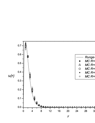
Figure 2: Reduced wave function for the ground state at $l=0$, and $\lambda=1$ and $\alpha=0.1$.

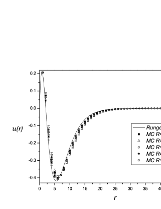
Figure 3: Same as Fig. 2, but for the first excited state.

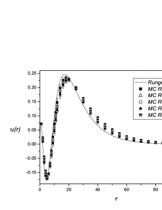
Figure 4: Same as Fig. 2, but for the second excited state.

$\alpha$	Quantum number $n$	Runge-Kutta/Numerov	MCH ($R\to 0$)
0.1	1	-0.4070	-0.4051 $\pm$ 0.0612
	2	-0.0499	-0.0463 $\pm$ 0.0069
	3	-0.0032	-0.0031 $\pm$ 0.0008
0.2	1	-0.3268	-0.3345 $\pm$ 0.0604
	2	-0.0121	-0.0120 $\pm$ 0.0036
0.3	1	-0.2576	-0.2453 $\pm$ 0.0584
0.4	1	-0.1984	-0.2069 $\pm$ 0.0545

Table 1: Comparison of some eigenvalues for $l=0$, $\lambda=1$, and some $\alpha$, between the Runge-Kutta/Numerov and MCH methods, where the MCH data have been extrapolated to the $R=0$ limit.

4 Critical Phenomena

As mentioned in Sec. 1, for a finite $\alpha$, the number of bound states is finite. Let us first take the system with $l=0$, $\lambda=1$ and $\alpha=0.1$ as an example. Figures 5 and 6 show the reduced wave function of the third excited state with $r_{max}=100$ and $r_{max}=200$ respectively. The location of the lowest valley goes further and further away from the origin, with increasing limit of integration $r_{max}$. It will goes to $r=\infty$ when $r_{max}\to\infty$. The eigenvalue $E$ for the third excited state is $8.1037\times 10^{-4}$ for $r_{max}=100$, $1.5533\times 10^{-4}$ for $r_{max}=200$, and $6.4491\times 10^{-5}$ for $r_{max}=300$. I.e., $E$ goes to zero when $r_{max}\to\infty$. Therefore the third excited state is no longer bounded. This also applies to higher states.

Figure 5: Reduced wave function for the third excited state at $l=0$, and $\lambda=1$ and $\alpha=0.1$, with $r_{max}=100$.

Figure 6: Same as Fig. 5, but with $r_{max}=200$.

	$\lambda=1$	$\lambda=2$	$\lambda=3$	$\lambda=4$	$\lambda=5$
$\alpha=0$	$\infty$	$\infty$	$\infty$	$\infty$	$\infty$
$\alpha=0.1$	3	5	6	7	7
$\alpha=0.2$	3	3	4	5	5
$\alpha=0.3$	2	2	3	3	3
$\alpha=0.4$	1	2	3	3	3
$\alpha=0.5$	1	2	2	3	3
$\alpha=0.6$	1	2	2	2	3
$\alpha\in[0.7,0.9]$	1	1	2	2	2
$\alpha\in[1.0,1.1]$	1	1	1	2	2
$\alpha=1.2$	-	1	1	2	2
$\alpha\in[1.3,1.4]$	-	1	1	1	2
$\alpha\in[1.5,2.3]$	-	1	1	1	1
$\alpha\in[2.4,3.5]$	-	-	1	1	1
$\alpha\in[3.6,4.7]$	-	-	-	1	1
$\alpha\in[4.8,5.9]$	-	-	-	1	1
$\alpha=6.0$	-	-	-	-	-

Table 2: Number of bound states at $l=0$ for various $\lambda$ and $\alpha$.

Table 2 shows the number of bound states for $l=0$ and various $\lambda$ and $\alpha$. From the table, we find that when $\alpha$ is sufficiently large, the attractive potential is so screened so that the system no longer has a bound state. The critical value for $\alpha$ is named critical screening parameter $\alpha_{C}$. After fine scanning $\alpha$ and studying the dependence of $u(r)$ on $r_{max}$, we obtain in Tab. 3 the value of $\alpha_{C}$ for $l=0$ and various $\lambda$. It is clear that $\alpha_{C}$ satisfy the relation

$$\alpha_{C}(l=0)=1.1906\lambda.$$ (10)

This tells us that the physics is the same for all $\lambda$, after rescaling the variables.

$\lambda$	1	2	3	4	5
$\alpha_{C}$	1.1906	2.3812	3.5718	4.7624	5.9530

Table 3: Dependence of $\alpha_{C}$ on $\lambda$ for $l=0$.

We have obtained the result of Tab. 3 by two criteria: (1) There is a unstable peak (or valley) in the ground wave function, with its location moving to $r\to\infty$ when $r_{max}\to\infty$; (2) The eigenvalue of the ground state becomes zero or positive as $r_{max}\to\infty$.

The second criterion is easy to understand for the $l=0$ case. In such a case, $U(r)=V(r)<0$. If the eigenvalue $E\geq 0$, then $q(r)$ in Eq. (4) becomes non-negative. According to QM, we know the state is unbounded. When $l\neq 0$, special care must be taken. Figures 7-9 plot $U(r)$ for $l\neq 0$ and various $\alpha$. When $\alpha<<\alpha_{C}$, as shown in Fig. 7, there is a well in $U(r)$, so that some bound states with $E<0$ might exist; Of course, a state with $E\geq 0$ is unbounded and the particle can travel to arbitrary large distance, because $q(r)$ is non-negative in the right hand side of the well. While $\alpha>>\alpha_{C}$, as shown in Fig. 9, the effective interaction is repulsive, and no bound state could exist.

Figure 7: $U(r)$ for $l\neq 0$ when $\alpha<<\alpha_{C}$.

Figure 8: $U(r)$ for $l\neq 0$ when $\alpha\approx\alpha_{C}$.

Figure 9: $U(r)$ for $l\neq 0$ when $\alpha>>\alpha_{C}$.

When $\alpha$ is equal to or just above $\alpha_{C}$, at which $U(r)$ behaves as Fig. 8, the second term in Eq. (3) dominates at intermediate and larger $r$. Is the state with eigenvalue $E=0+$ bounded? Without sufficiently large $r_{max}$, one would conclude that the state with $E=0+$ to be bounded. However, with sufficiently large $r_{max}$, $q(r)$ becomes non-negative at large $r$, and the particle can penetrate the well and goes to $r\to\infty$ through tunnelling. This means the state with $E=0+$ is actually not a bound state.

One should look into the wave function in great detail. Let us take $l=4$, $\lambda=1$, and $\alpha=0.03135$ as an example. $U(r)$ behaves like Fig. 8. When $r_{max}\in[300,4267)$, the system seems to have a bounded ground state with $E\approx 1.84\times 10^{-6}$. The reduced wave function of the ground state is shown in Fig. 10; The wave function and energy are stable within this range of $r_{max}$. However, when $r_{max}\geq 4267$, as shown in Fig. 11, a peak in $u(r)$ at large $r$ appears. The location of this peak goes to $r\to\infty$ as increasing $r_{max}$, at the same time, the energy of the state also tends to zero. Therefore, there is no ground state for $l=4$, $\lambda=1$, and $\alpha=0.03135$.

Figure 10: Reduced wave function for the ground state with $l=4$, $\lambda=1$, $\alpha=0.03135$ and $r_{max}<4267$.

Figure 11: Same as Fig. 10, but with $r_{max}=4267$.

Table 4 lists the value of $\alpha_{C}$ for various $l$, where $k_{l}$ is defined by

$$k_{l}={\alpha_{C}(l)\over\lambda}.$$ (11)

Figure 12 shows $k_{l}$ as a function of $l$. We can fit the data by

$$k_{l}=A_{1}\exp(-{l\over B_{1}})+A_{2}\exp(-{l\over B_{2}}),$$ (12)

with the fitting parameters given in Tab. 5. For small $l$, the first term is dominant because $A_{1}>A_{2}$. While for larger $l$, the second term is dominant, because $B_{1}<B_{2}$. This implies that $\alpha_{C}$ decays exponentially for large $l$.

$l$	0	1	2	3	4	5
$k_{l}$	1.1906	0.2202	0.0913	0.0498	0.0313	0.0215
$l$	6	7	8	9	10
$k_{l}$	0.0157	0.0119	0.0094	0.0076	0.0063

Table 4: Dependence of $k_{l}$ on $l$.

Figure 12: $k_{l}$ as a function of $l$.

fitting coefficient	$A_{1}$	$B_{1}$	$A_{2}$	$B_{2}$
data	1.020	0.443	0.170	2.490
error	0.018	0.014	0.017	0.180

Table 5: Fitting parameters in Eq. (12).

5 Discussions

In the preceding sections, we have systematically investigated the bound states and critical phenomena of the Yukawa potential, by means of different numerical algorithms. The results for the critical screening $\alpha_{C}$ are consistent with the literature. We also obtain a new relation between $\alpha_{C}$ and the angular momentum $l$.

When judging whether a state is bounded, one must carefully study the effects of the boundary $r_{max}$ on the wave function and energy. We believe such an experience might be very useful for numerical study of quantum theory, in particular at criticality.

While the Runge-Kutta/Numerov algorithm works better in 1D QM, it does not work in quantum field theory. In this case, the Monte Carlo methods play an important role. The Monte Carlo Hamiltonian method has been tested as a useful method for computing the wave function and spectrum beyond the ground state, at least in QM and the scalar lattice field theory. We believe that the extension to QCD will allow to explore more useful information on strong interactions.

Acknowledgments

We thank K Schmidt for useful discussions.

References

- [1] H. Yukawa, Proc. Phys. Math. Soc. Jap. 17 (1935) 48.
- [2] R. Sachs, and M. Goeppert-Mayer, Phys. Rev. 53 (1938) 991.
- [3] G.M. Harris, Phys. Rev. 125 (1962) 1131.
- [4] H. Schey, and J. Schwartz, Phys. Rev. 139 (1965) B1428.
- [5] J. Rogers, H. Graboske, and E. Harwood, Phys. Rev. A1 (1970) 1577.
- [6] J. McEnnan, L. Kissel, and R. Pratt, Phys. Rev. A13 (1976) 532.
- [7] C. Gerry, J. Phys. A17 (1984) L313.
- [8] H. Kröger, R. Girard, and G. Dufour, Phys. Rev. C37 (1988) 486.
- [9] R. Girard, H. Kröger, P. Labelle and Z. Bajzer, Phys. Rev. A 37 (1988) 3195.
- [10] S. Garavelli, and F. Oliveira, Phys. Rev. Lett. 66 (1991) 1310.
- [11] O. Gomes, H. Chacham, and J. Mohallem, Phys. Rev. A50 (1994) 228.
- [12] V. I. Yukalov, E. P. Yukalova and F. A. Oliveira, J. Phys. A 31 (1998) 4337.
- [13] F. Brau, J. Phys. A36 (2003) 9907.
- [14] L. Bertini, M. Mella, D. Bressanini, and G. Morosi, Phys. Rev. A69 (2004) 042504.
- [15] D. Dean, I. Drummond, and R. Horgan J. Phys. A37 (2004) 2039.
- [16] S. De Leo and P. Rotelli, Phys. Rev. D 69 (2004) 034006.
- [17] S. Khrapak, A. Ivlev, G. Morfill, and S. Zhdanov, Phys. Rev. Lett. 90 (2003) 225002.
- [18] L. Iorio, Phys. Lett. A298 (2002) 315.
- [19] E. B. Gregory, S. H. Guo, H. Kröger and X. Q. Luo, Phys. Rev. D 62 (2000) 054508.
- [20] X. Q. Luo, E. B. Gregory, S. H. Guo and H. Kröger, in Non-perturbative methods and lattice QCD, World Scientific, Singapore (2001) 138. hep-ph/0011120.
- [21] Y.Z. Fang and X. Q. Luo, Phys. Rev. D 69 (2004) 114501.
- [22] X. Q. Luo, Phys. Rev. D 70 (2004) 091504 (Rapid Commun.).
- [23] W. Press, S. Teukolsky, W. Vetterling, B. Flannery, “Numerical Recipes in C”, (Cambridge University Press, 1992).
- [24] H. Jirari, H. Kroger, X. Q. Luo and K. J. M. Moriarty, Phys. Lett. A 258 (1999) 6.
- [25] N. Metropolis, A. W. Rosenbluth, M. N. Rosenbluth, A. H. Teller and E. Teller, J. Chem. Phys. 21 (1953) 1087.
- [26] X.Q. Luo, and Q. Chen, Mod. Phys. Lett. A11 (1996) 2435.
- [27] X.Q. Luo, Q. Chen, S. Guo, X. Fang, and J. Liu, Nucl. Phys. B (Proc. Suppl.)53 (1997) 243.
- [28] X. Q. Luo, C. Q. Huang, J. Q. Jiang, H. Jirari, H. Kroger and K. J. M. Moriarty, Physica A 281 (2000) 201.
- [29] X. Q. Luo, C. Q. Huang, J. Q. Jiang, H. Jirari, H. Kroger and K. J. M. Moriarty, Nucl. Phys. B(Proc. Suppl.) 83 (2000) 810.
- [30] H. Jirari, H. Kroger, C. Q. Huang, J. Q. Jiang, X. Q. Luo and K. J. M. Moriarty, Nucl. Phys. B(Proc. Suppl.) 83 (2000) 953.
- [31] J. Q. Jiang, C. Q. Huang, X. Q. Luo, H. Jirari, H. Kroger and K. Moriarty, Commun. Theor. Phys. 34 (2000) 723.
- [32] C. Huang, J. Jiang, X. Q. Luo, H. Jirari, H. Kroger and K. Moriarty, High Energy Phys. Nucl. Phys. 24 (2000) 478.
- [33] X. Q. Luo, H. Xu, J. Yang, Y. Wang, D. Chang, Y. Lin and H. Kroger, Commun. Theor. Phys. 36 (2001) 7.
- [34] X. Q. Luo, J. J. Liu, C. Q. Huang, J. Q. Jiang and H. Kroger, Commun. Theor. Phys. 38 (2002) 561.
- [35] X. Q. Luo, H. Jirari, H. Kroger and K. J. Moriarty, in Non-perturbative methods and lattice QCD, World Scientific, Singapore (2001) 100. hep-lat/0108026.
- [36] C. Q. Huang, X. Q. Luo, H. Kroger and K. J. Moriarty, Phys. Lett. A299 (2002) 483.
- [37] H. Kroger, X. Q. Luo and K. J. Moriarty, Nucl. Phys. B(Proc. Suppl.)119 (2003) 508.
- [38] H. Kroger, X. Q. Luo and K. J. Moriarty, Math. Comput. Simul. 62 (2003) 377.
- [39] R.P. Feynman and A.R. Hibbs, Quantum Mechanics and Path Integrals, (McGraw-Hill, New York, 1965).
- [40] X. Q. Luo, X. N. Cheng and H. Kroger, Commun. Theor. Phys. 41 (2004) 509.