1 Introduction

QCD is a theory which gives rise to extremely diverse phenomena depending on the energy range which is involved. At low energies ($E\mathrel{\raise 2.58334pt\hbox{$<$}\kern-7.7778pt\lower 2.79857pt\hbox{$\sim$}}1$ GeV) the physics is non perturbative and it is in many aspects strongly influenced by chiral symmetry. Chiral symmetry is a global symmetry of the QCD Lagrangian (as we will discuss in detail) in the case where $N^{0}_{F}\geq 2$ quarks are massless and it happens that the vacuum of this theory breaks the symmetry spontaneously, a fact which is linked to confinement. Physically, this property is relevant because some of the quarks happen to be very light, with a mass much smaller than 1 GeV, such that they do probe, in a sense, the chiral vacuum. The method of chiral perturbation theory (ChPT) exploits this property of QCD in a general and systematic way. These lectures are an introduction to this subject at a basic level which could help the reader in tackling, later on, the classic papers on this subject[1][2][3]. For a rather complete introduction one may consult the recent review[4]. A detailed description of applications can be found in the book[5] and, for the quantum field theoretical aspects, of course, one should consult Weinberg’s book[6].

2 Symmetries of chiral QCD

The field content of QCD consists of a set of 8 massless gluon fields $G^{a}_{\mu}$ associated with the $SU_{c}(3)$ colour gauge group and a set of six quarks $q_{f}$. The mass pattern of the quarks is remarkable and is displayed below

$f$	$q_{f}$	$m_{f}$ ( MeV)
1	u	$\sim$ 5
2	d	$\sim$ 7
3	s	$\sim$ 100
4	c	$\sim$ 1200
5	b	$\sim$ 4200
6	t	$\sim$ 174000

The masses are “running” parameters i.e they depend on a scale $\mu$ (for the light quarks the numbers above correspond to $\mu=2$ GeV). At present, the determination of the masses is very approximate (see e.g.[7]). One of the goals of the chiral expansion is to extract informations on the values of lightest three quarks from experiment. The numbers above suggest to divide the quarks into a group of “light” quarks, $f\leq 3$ and a group of heavy quarks for $f\geq 4$. The chiral expansion is an effective Lagrangian technique which generates an expansion in powers of the light quark masses, $m_{f}$ divided by a scale $\Lambda$ which is expected to be of the order of 1 GeV. This expansion is completely non perturbative with respect to the QCD running coupling constant $g_{s}$ and will necessitates that one makes a change from the quark and gluon fields to a new set of variables.

2.1 Identification of the symmetries

As a first step, let us write the QCD Lagrangian in the following form

$${\cal L}_{QCD}={\cal L}^{0}_{QCD}+{\cal L}^{sources}_{QCD}$$ (1)

with

$${\cal L}^{0}_{QCD}=-{1\over 4}G^{a}_{\mu\nu}G^{a\,\mu\nu}+\sum_{f={N^{0}_{F}+1}}^{6}\bar{q}_{f}(i\gamma^{\mu}D_{\mu}-m_{f})q_{f}$$

$$\phantom{{\cal L}^{0}_{QCD}=}+\sum_{f=1}^{N^{0}_{F}}\bar{q}_{f}\gamma^{\mu}(iD_{\mu})q_{f}\ .$$ (2)

Here, $D_{\mu}$ is the covariant derivative

$$iD_{\mu}=i\partial_{\mu}+g_{s}G^{a}_{\mu}{T^{a}}\ .$$ (3)

with $T^{a}$ being the eight generators of the $SU_{c}(3)$ colour group (i.e. $T^{a}=\lambda^{a}/2$, $\lambda^{a}$ are the Gell-Mann matrices). The quark fields must be considered as 3-vectors in colour space. In this formula, the quark flavours with $f\geq{N^{0}_{F}+1}$ are the ones which we decide to treat as heavy. We note that ${\cal L}^{0}_{QCD}$ does not contain any mass term for the quarks with flavour index $f\leq{N^{0}_{F}}$, which we will call the light quarks. There is some freedom in the choice of ${N^{0}_{F}}$, one can take ${N^{0}_{F}}=2$ or ${N^{0}_{F}}=3$. For definiteness, we will assume ${N^{0}_{F}}=3$ in the following. The mass terms of the light quarks are included in the second piece ${\cal L}^{sources}_{QCD}$ which we will discuss in detail later. This piece will also account for the couplings of the quarks to the other fields in the standard model. The piece ${\cal L}^{0}_{QCD}$ is to be treated exactly: the dynamics will be reflected in the values of sets of low-energy coupling constants. The piece ${\cal L}^{sources}_{QCD}$ will be treated perturbatively.

For the moment, let us examine the symmetry properties of ${\cal L}^{0}_{QCD}$. We recall the basic properties of the Dirac gamma matrices

$$\{\gamma_{\mu},\gamma_{\nu}\}=2g_{\mu\nu},\quad\{\gamma_{\mu},\gamma_{5}\}=0$$ (4)

A particular representation for these matrices is

$$\gamma_{0}=\left(\begin{array}[]{cc}0&-\mathbf{1}\\ -\mathbf{1}&0\\ \end{array}\right),\ \gamma_{i}=\left(\begin{array}[]{cc}0&\sigma_{i}\\ -\sigma_{i}&0\\ \end{array}\right),\ \gamma_{5}=\left(\begin{array}[]{cc}\mathbf{1}&0\\ 0&-\mathbf{1}\\ \end{array}\right)\ .$$ (5)

The entries there are 2x2 matrices and $\sigma_{i}$ are the three Pauli matrices. Chiral symmetry is a group of transformations which acts on the light quark fields. The heavy quark fields as well as the gluon fields are unaffected by these transformations. In order to see how these transformations operate let us form a $N_{F}^{0}$–components vector from the $N_{F}^{0}$ light quarks, with $N_{F}^{0}=3$, for instance

$$\psi=\left(\begin{array}[]{c}u\\ d\\ s\\ \end{array}\right)\ .$$ (6)

Next, let us introduce two projectors

$$P_{L}={1-\gamma^{5}\over 2},\quad P_{R}={1+\gamma^{5}\over 2}\ .$$ (7)

It is easily verified that the projectors satisfy the following properties

$$P_{L}+P_{R}=1,\quad P_{L}^{2}=P_{L},\quad P_{R}^{2}=P_{R}$$

$$P_{L}P_{R}=P_{R}P_{L}=0,\quad\gamma_{\mu}P_{L}=P_{R}\gamma_{\mu},\quad\gamma_{\mu}P_{R}=P_{L}\gamma_{\mu}$$ (8)

With the help of these we define projected spinor fields

$$\psi_{L}=P_{L}\psi,\quad\psi_{R}=P_{R}\psi$$ (9)

and, using that $\bar{\psi}=\psi^{\dagger}\gamma^{0}$

$$\bar{\psi}_{L}=\bar{\psi}P_{R},\quad\bar{\psi}_{R}=\bar{\psi}P_{L}\ .$$ (10)

The projected spinors are eigenstates of “chirality”

$$\gamma^{5}\psi_{L}=-\psi_{L},\quad\gamma^{5}\psi_{R}=\psi_{R}\ .$$ (11)

Using the representation (5) above for the gamma matrices these projected spinors can be associated with two-component spinors $\tilde{\psi}_{L}$ and $\tilde{\psi}_{R}$ (called Weyl spinors)

$$\psi_{L}=\left(\begin{array}[]{c}0\\ \tilde{\psi}_{L}\\ \end{array}\right)\quad\psi_{R}=\left(\begin{array}[]{c}\tilde{\psi}_{R}\\ 0\\ \end{array}\right)$$ (12)

In the absence of interactions the projected spinors are also eigenstates of helicity. Starting from the free Dirac equation, and considering positive-energy plane-waves $\tilde{\psi}_{L}(x)=\exp(-ipx)\tilde{\psi}_{L}(p)$, $\tilde{\psi}_{R}(x)=\exp(-ipx)\tilde{\psi}_{R}(p)$, indeed, one easily finds that $\tilde{\psi}_{L}(p)$ and $\tilde{\psi}_{R}(p)$ correspond to states with a left-handed and a right-handed helicity respectively,

$$\vec{\sigma}\cdot\widehat{p}\,\tilde{\psi}_{L}(p)=-\tilde{\psi}_{L}(p)\ ,\quad\vec{\sigma}\cdot\widehat{p}\,\tilde{\psi}_{R}(p)=\tilde{\psi}_{R}(p)\ .$$ (13)

The key feature of ${\cal L}^{0}_{QCD}$ is that, using eqs.(2.1), we can rewrite the massless quark part as two independent pieces in terms of $\psi_{L}$ and $\psi_{R}$,

$${\cal L}_{QCD}^{chir}\equiv\bar{\psi}i\gamma^{\mu}D_{\mu}\psi=\bar{\psi}(P_{L}+P_{R})i\gamma^{\mu}D_{\mu}(P_{L}+P_{R})\psi={\cal L}_{QCD}^{L}+{\cal L}_{QCD}^{R}$$ (14)

with

$${\cal L}_{QCD}^{L}=\bar{\psi}_{L}i\gamma^{\mu}D_{\mu}\psi_{L},\quad{\cal L}_{QCD}^{R}=\bar{\psi}_{R}i\gamma^{\mu}D_{\mu}\psi_{R}\ .$$ (15)

It is important to note that the decomposition (14) holds in QCD because the gluons are vector particles (and not scalars or tensors). Let $g_{L}$ be a $N_{F}^{0}\times N_{F}^{0}$ matrix and let us perform the transformation

$$\psi_{L}\to\,g_{L}\psi_{L},\ \bar{\psi}_{L}\to\bar{\psi}_{L}\,g_{L}^{\dagger}$$ (16)

(we recall that according to eq.(6) $\psi_{L}$ is a $N_{F}^{0}$ components vector) while $\psi_{R}$ is unaffected. We see that the Lagrangian (14) is left invariant by this transformation provided that the matrices $g_{L}$ satisfy

$$g_{L}^{\dagger}\,g_{L}=I\ .$$ (17)

In other terms $g_{L}$ must be a unitary matrix. The Lagrangian (14) is thus found to be invariant under transformations by a group of unitary matrices which we may call $U_{L}(3)$ acting on $\psi_{L}$. Obviously, the Lagrangian is also invariant under a group of unitary matrices acting on $\psi_{R}$. The complete invariance group of ${\cal L}^{0}_{QCD}$ is therefore

$$U_{L}(N_{F}^{0})\times U_{R}(N_{F}^{0})\ .$$ (18)

We can parametrize an arbitrary element of this group in the following way

$$(g_{L},g_{R})=({\rm e}^{i\alpha}{\rm e}^{i\beta}{\rm e}^{i\alpha^{l}T^{l}}{\rm e}^{i\beta^{l}T^{l}},{\rm e}^{i\alpha}{\rm e}^{-i\beta}{\rm e}^{i\alpha^{l}T^{l}}{\rm e}^{-i\beta^{l}T^{l}})$$ (19)

in terms of $2(N_{F}^{0})^{2}$ real parameters. This expression shows that one can factor out two $U(1)$ groups, such that one can write

$$U_{L}(N_{F}^{0})\times U_{R}(N_{F}^{0})=U_{V}(1)\times U_{A}(1)\times SU_{L}(N_{F}^{0})\times SU_{R}(N_{F}^{0})\ .$$ (20)

One can also verify that the ensemble of matrices which have the form

$$(g,g)=({\rm e}^{i\alpha^{l}T^{l}},{\rm e}^{i\alpha^{l}T^{l}})$$ (21)

form a subgroup which we will label as $SU_{V}(N_{F}^{0})$. The set of matrices of the form

$$(h,h^{\dagger})=({\rm e}^{i\beta^{l}T^{l}},{\rm e}^{-i\beta^{l}T^{l}})$$ (22)

are called axial transformations, this set does not form a group. It is useful to note how the spinor $\psi=\psi_{L}+\psi_{R}$ transforms under a vector and an axial transformation. Starting from eq.(16) and the similar one for $\psi_{R}$ it is easy to deduce

$$V:\psi\to{\rm e}^{i\alpha^{l}T^{l}}\psi\quad\ A:\psi\to{\rm e}^{i\beta^{l}T^{l}\gamma^{5}}\psi\ .$$ (23)

2.2 Consequences of the symmetries

According to Noether’s theorem, to each parameter of a continuous symmetry corresponds a current $J_{\mu}(x)$ which is conserved, i.e. satisfies $\partial^{\mu}J_{\mu}(x)=0$ (see e.g. [6]). The method for obtaining the explicit form of the current is standard. In the present case, we consider $\psi(x)$ fields which are solutions of the classical equations of motion, such that the action is invariant under arbitrary infinitesimal variations $\delta\psi(x)$ to first order. Then we generate variations associated with chiral transformations with infinitesimal values of the parameters $\alpha$, $\beta$, $\alpha_{l}$, $\beta_{l}$, taken to be $x$ dependent. For instance, in order to obtain the axial current we perform the variation

$$\delta\psi(x)=i\beta^{l}(x)T^{l}\gamma^{5}\psi(x),\quad$$ (24)

for arbitrary infinitesimal $\beta^{l}(x)$ and use the fact that $\delta S^{0}_{QCD}=0$. In this way one easily obtains the form of the vector and axial-vector currents,

$$V_{\mu}^{0}=\bar{\psi}\gamma_{\mu}\psi,\quad V_{\mu}^{a}=\bar{\psi}\gamma_{\mu}{\lambda^{a}\over 2}\psi,\quad A_{\mu}^{a}=\bar{\psi}\gamma_{\mu}\gamma_{5}{\lambda^{a}\over 2}\psi,\quad\ .$$ (25)

The singlet axial-vector current $A_{\mu}^{0}$ is also conserved at the classical level, but the conservation law $\partial^{\mu}A_{\mu}^{0}=0$ turns out to be modified in $QCD$ by quantum mechanical effects (this is the famous ABJ anomaly[9] ). This was analyzed in detail by ’t Hooft ref.[10] and the result is that the $U_{A}(1)$ group is not a symmetry of ${\cal L}^{0}_{QCD}$ at the quantum level.

In addition to this continuous symmetry group, the $QCD$ action is invariant under the discrete symmetries of parity, charge conjugation and time reversal invariance. Starting from the representation in terms of Weyl spinors,

$$\psi(t,\vec{x})=\left(\begin{array}[]{l}\tilde{\psi}_{R}(t,\vec{x})\\ \tilde{\psi}_{L}(t,\vec{x})\end{array}\right)$$ (26)

let us recall how $P$ and $C$, for instance, act (see e.g. [6]),

$$P:\psi\to\left(\begin{array}[]{l}\tilde{\psi}_{L}(t,-\vec{x})\\ \tilde{\psi}_{R}(t,-\vec{x})\end{array}\right),\quad C:\psi\to\left(\begin{array}[]{l}\sigma_{2}\tilde{\psi}_{L}^{*}(t,\vec{x})\\ -\sigma_{2}\tilde{\psi}_{R}^{*}(t,\vec{x})\end{array}\right)$$ (27)

The action of both $C$ and $P$ acting on the chiral part of the QCD Lagrangian (see (14) ), ${\cal L}^{chir}_{QCD}$ is to interchange the parts ${\cal L}^{L}_{QCD}$ and ${\cal L}^{R}_{QCD}$.

At this point we may start to ask ourselves about the consequences of this symmetry concerning the spectrum of bound states of QCD. The important issue will be to know whether the ground state of QCD (i.e. the vacuum) is also invariant under the full chiral group or not. Let us first assume that the vacuum is fully invariant: the expectation then (still ignoring the small effect of light quark masses) is that the spectrum will consist of degenerate double $SU(3)$ multiplets of opposite parity. Let us show this, for example, in the case of the vector and the axial vector mesons. Let us consider the correlator

$$\Pi_{\mu\nu}^{+-}=<0|TV^{+}_{\mu}(x)V^{-}_{\nu}(0)|0>,\quad V^{\pm}_{\mu}(x)=\bar{\psi}(x){\lambda_{1}\pm i\lambda_{2}\over 2}\gamma^{\mu}\psi(x)\ .$$ (28)

Firstly, using invariance of the vacuum under $SU_{V}(3)$ transformations

$${\rm e}^{i\alpha^{l}Q^{l}_{V}}|0>=|0>$$ (29)

one can derive that the correlators are flavour symmetric, i.e. for any two flavour indices $i,j$ the correlator must be of the form

$$\Pi_{\mu\nu}^{ij}={1\over 2}\delta^{ij}\Pi_{\mu\nu}^{+-}\ .$$ (30)

Next, let us also assume invariance of the vacuum under the axial transformation

$${\rm e}^{i\beta Q^{3}_{A}}|0>=|0>\ .$$ (31)

This implies

$$<0|TV^{+}_{\mu}(x)V^{-}_{\nu}(0)|0>=<0|{\rm e}^{-i\beta Q^{3}_{A}}TV^{+}_{\mu}(x)V^{-}_{\nu}(0){\rm e}^{i\beta Q^{3}_{A}}|0>=<0|TV^{{}^{\prime}+}_{\mu}(x)V^{{}^{\prime}-}_{\nu}(0)|0>$$ (32)

where

$$V^{{}^{\prime}+}_{\mu}(x)=\bar{\psi}^{\prime}(x){\lambda_{1}\pm i\lambda_{2}\over 2}\gamma^{\mu}\psi^{\prime}(x),\quad\psi^{\prime}(x)={\rm e}^{i\beta{\lambda^{3}\over 2}\gamma^{5}}\psi(x)\ .$$ (33)

Expanding up to quadratic order in the parameter $\beta$ we get

$$V^{{}^{\prime}+}_{\mu}(x)=V^{+}_{\mu}(x)+i\beta A^{+}_{\mu}(x)-{1\over 2}\beta^{2}V^{+}_{\mu}(x)$$

$$V^{{}^{\prime}-}_{\mu}(x)=V^{-}_{\mu}(x)-i\beta A^{-}_{\mu}(x)-{1\over 2}\beta^{2}V^{-}_{\mu}(x)\ .$$ (34)

Replacing in eq.(32) and collecting the terms quadratic in $\beta$ we obtain that the correlator of vector currents is identical to the correlator of axial-vector currents

$$<0|TV^{+}_{\mu}(x)V^{-}_{\nu}(0)|0>=<0|TA^{+}_{\mu}(x)A^{-}_{\nu}(0)|0>\ .$$ (35)

Eq.(35) implies that the vector and axial-vector mesons should form mass degenerate multiplets. One could repeat the same argument using scalar and pseudo-scalar currents baryon currents etc… However, this is not what is observed experimentally: while such multiplets exist, the axial-vectors are much heavier than the vectors. The reason for this behaviour is that while the QCD Lagrangian is invariant under the chiral symmetry group the ground state of the theory is not invariant under the full group (one says that there is spontaneous breakdown of this part of the symmetry group). The possibility of such a behaviour in field theory was pointed out by Nambu and by Goldstone[11]. An important implication which they noted is the related existence of massless particles, now referred to as the Nambu-Goldstone bosons. We will illustrate this property, which is crucial for the low energy properties of QCD and the chiral expansion method, in the next section. Before that, let me simply state a set of nice results which have been proved in the case of QCD.
a) The subgroup $SU_{V}(N_{F}^{0})$ of the chiral group cannot be spontaneously broken[12].
b) The lightest particles in the QCD spectrum are pseudoscalar mesons[13]
c) Assuming that QCD with $N^{0}_{F}$ massless quarks confines, then, in the case $N^{0}_{F}\geq 3$, one can show that the QCD spectrum must contain massless boson states in order to properly satisfy the so called anomaly matching conditions[14]. These bosons, according to the result b) must be pseudoscalar bosons. This last result implies that symmetry under the axial transformations must undergo spontaneous breakdown in QCD. It is however not excluded that a discrete axial subgroup could remain unbroken.

3 Illustration of spontaneous symmetry breaking

3.1 A spin model

We first illustrate with a simple lattice model that in a system with an infinite number of variables, the possibility that spontaneous breakdown of a symmetry occurs is rather natural. Let us consider a system of spins, represented as 3-vectors of unit length, located on the sites of an infinite dimensional lattice. The Hamiltonian of this system is taken to be

$$H=J\sum\vec{S}_{i}.\vec{S}_{j}$$ (36)

where the sum extends, say, over nearest neighbours. The Hamiltonian is invariant under the transformations $\vec{S}_{i}\to g\vec{S}_{i}$ which leave the scalar product invariant, i.e. $g$ belongs to the group of 3-dimensional rotations $O(3)$. Concerning the ground state of the system, we have two possibilities

• the system is disordered

• the system is ordered.

As an example of the latter possibility we may have all the spins aligned along a given direction which would correspond to a ferromagnetic system. This is illustrated in fig.1 below.

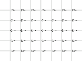
Figure 1: Ordered ground state corresponding to a ferromagnetic system.

In this case, the ground state is not invariant under the symmetry group $O(3)$ it is invariant under the subgroup of rotations perpendicular to the $x-$axis, that is, an $O(2)$ group. Alternatively, the ground state of the system may be disordered, i.e. the directions of the spins are randomly distributed. This is illustrated in fig.2.

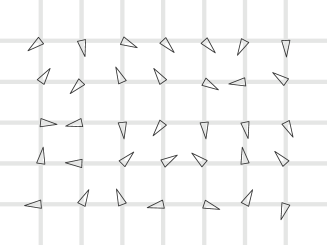
Figure 2: Disordered ground state.

In this case, the aspect of the system will appear to be the same for an observer in any reference frame. In particular, the ground state is invariant under the same symmetry group $O(3)$ as the Hamiltonian (36). We may characterize the nature of the ground state by an order parameter. For instance, we may choose the average value of the spin along the $x-$axis as an order parameter

$$M_{1}=<S^{x}>={1\over N}\sum_{i}{S^{x}_{i}}$$ (37)

Obviously, $M_{1}$ vanishes if the state is disordered, as in fig.2 and it is non-vanishing in the case of the ferromagnetic state. More complicated forms of order are also possible. For instance, fig.3 illustrates the case of an anti-ferromgnetic ground state.

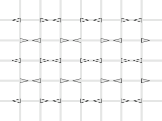
Figure 3: Ordered ground state corresponding to a anti-ferromagnetic system.

In this case, the state is invariant under the group $O(2)$ of rotations perpendicular to the $x-$axis and also under the change of $x$ into $-x$ so the full symmetry group is $O(2)\times Z_{2}$. The order parameter $M_{1}$ vanishes for this state but we can imagine a more complicated order parameter

$$M_{2}={1\over N}\sum S^{x}_{i}S^{x}_{i+1}$$ (38)

which does not, while $M_{2}$ would still vanish in the case of a disordered ground state. Analogous situations in the case of QCD were discussed in refs.[15] and [16].

3.2 The linear sigma model

Now we consider a continuous model, the classic linear sigma model[17] and we will investigate in more details the dynamics of the fluctuations around the ground state. The dynamical degrees of freedom consist of four real-valued scalar fields $\phi_{a}(x)$ which can be collected into a four-component vector $\tilde{\phi}(x)$ and the dynamics is defined from the following Lagrangian,

$${\cal L}_{lsm}={1\over 2}\partial_{\mu}\tilde{\phi}(x)\cdot\partial^{\mu}\tilde{\phi}(x)+{\mu\over 2}\tilde{\phi}(x)\cdot\tilde{\phi}(x)-{\lambda\over 4}(\tilde{\phi}(x)\cdot\tilde{\phi}(x))^{2}$$ (39)

One must have $\lambda>0$ otherwise the Hamiltonian would not be bounded from below and $\mu$ can have either sign. The Lagrangian is invariant under transformations of the four-vector $\tilde{\phi}$

$$\tilde{\phi}\to G\tilde{\phi}$$ (40)

where $G$ belongs to the orthogonal group $O(4)$. One can reformulate the model such that the global symmetry resembles the one in QCD. For this purpose, let us map the four vector to a $2\times 2$ matrix $\Sigma$

$$\Sigma=\phi_{0}+i\vec{\tau}\cdot\vec{\phi}\ .$$ (41)

In terms of $\Sigma$ the Lagrangian can be written as follows,

$${\cal L}_{lsm}={1\over 4}{\rm tr\,}(\partial_{\mu}\Sigma\partial^{\mu}\Sigma^{\dagger})+{\mu\over 4}{\rm tr\,}(\Sigma\Sigma^{\dagger})-{\lambda\over 16}({\rm tr\,}(\Sigma\Sigma^{\dagger}))^{2}\ .$$ (42)

In this form, the invariance group appears to be $SU(2)\times SU(2)$ with

$$\Sigma\to g\Sigma h^{\dagger}$$ (43)

which resembles the case of $QCD$ with $N^{0}_{F}=2$.

Let us now consider the ground state $\psi_{0}$ of this system. By analogy with the spin system considered above we may choose the expectation values of the components of $\tilde{\phi}$ as order parameters. By a suitable redefinition we can always arrange that the expectation value of the $\phi_{0}$ component

$$<\Psi_{0}|\phi_{0}|\Psi_{0}>\equiv\bar{\phi}_{0}$$ (44)

may or may not be vanishing while the other expectation values $\bar{\phi}_{i},i=1,2,3$ are always vanishing. In a semi-classical approximation $\bar{\phi}_{0}$ is given simply by solving the classical equations of motion for $\phi_{0}$ (this can be seen easily using the path integral formalism). Because of translational invariance of the vacuum $\bar{\phi}_{0}$ is independent of $x$ and the equations of motion simply read

$$\bar{\phi}_{0}(\mu-\lambda\bar{\phi}_{0}^{2})=0\ .$$ (45)

If $\mu<0$ the only solution is $\bar{\phi}_{0}=0$ which corresponds to a disordered vacuum, invariant under the full symmetry group. If $\mu>0$ there are solutions with $\bar{\phi}_{0}\neq 0$,

$$\bar{\phi}_{0}=\pm\sqrt{\mu\over\lambda}\ .$$ (46)

Fig. 4 shows that these are the stable solutions. In this case, the subgroup $SU_{V}(2)$ of transformations with elements of the form $(g,g)$ leave the vacuum invariant

$$g\bar{\phi}_{0}g^{\dagger}=\bar{\phi}_{0}$$ (47)

while the set of axial transformations $(h,h^{\dagger})$ do not

$$h\bar{\phi}_{0}h\neq\bar{\phi}_{0}\ .$$ (48)

\psfrag{energy}{$<H>$ }\psfrag{phi0bar}{$\bar{\phi}_{0}$}\includegraphics[width=284.52756pt]{lsmvac}

Figure 4: Value of the Hamiltonian as a function of $\bar{\phi}_{0}$.

Correspondingly, we expect the appearance of three massless states: this is Goldstone theorem. The theorem holds in the absence of gauge fields coupling to these states and can be proved quite generally [18]. We will verify this in the semi-classical approximation: for this purpose, we consider small fluctuations around the classical solution. One way to perform this is to write the $\Sigma$ field as,

$$\Sigma=\bar{\phi}_{0}+\phi_{0}+i\vec{\tau}.\vec{\phi}\ .$$ (49)

We will choose, however, the following alternative parametrization for the fluctuations

$$\Sigma=(\bar{\phi}_{0}+\sigma)U,\quad U=\exp\left({i\vec{\tau}\vec{\pi}\over\bar{\phi}_{0}}\right)\ .$$ (50)

The parametrization (49) is the most convenient one if we want to perform an ordinary perturbative expansion (i.e. an expansion in powers of the coupling constant $\lambda$). The alternative parametrization will allow us to perform a radically different kind of expansion: the chiral expansion. Replacing in the Lagrangian(42) one obtains,

$${\cal L}_{lsm}={1\over 4}(\bar{\phi}_{0}+\sigma)^{2}\langle\partial_{\mu}U\partial^{\mu}U^{\dagger}\rangle$$ (51)

$$\phantom{{\cal L}_{lsm}=}+{1\over 2}\partial_{\mu}\sigma\partial^{\mu}\sigma++{\mu\over 2}(\bar{\phi}_{0}+\sigma)^{2}-{\lambda\over 4}(\bar{\phi}_{0}+\sigma)^{4}\ .$$ (52)

One observes that no mass term appears in this Lagrangian for the three pions $\pi_{a}$, this is in accordance Goldstone theorem. In addition, one has a $\sigma$ meson, which is massive,

$$m_{\sigma}^{2}=2\mu\ .$$ (53)

One notices from (51) that the strength of the interaction among pions vanishes for vanishing momenta, such that for small pion momenta we have a weakly coupled system. The main idea of the chiral expansion is that if we confine ourselves to a range of energies (or momenta) for the pions which is much smaller than $m_{\sigma}$ we can “integrate out” the sigma field. In this way we can describe the dynamics of pions as an expansion in powers of the momenta. For this purpose, let us introduce a chiral counting rule: we count the term $\langle\partial_{\mu}U\partial^{\mu}U^{\dagger}\rangle$ as $O(p^{2})$ since it involves two derivatives of the pion field. How do we count the $\sigma$ field ? We expect it to be a small fluctuation so let us count it as $O(p^{2})$ also. These rules automatically give rise to an expansion. To begin with, we have a single term of order $O(p^{2})$,

$${\cal L}^{(2)}={1\over 4}(\bar{\phi}_{0})^{2}\langle\partial_{\mu}U\partial^{\mu}U^{\dagger}\rangle\ .$$ (54)

At $O(p^{4})$, at the classical level we must keep terms linear and quadratic in the sigma field,

$${\cal L}^{(4)}={1\over 2}\bar{\phi}_{0}\sigma\langle\partial_{\mu}U\partial^{\mu}U^{\dagger}\rangle-{1\over 2}m_{\sigma}^{2}\sigma^{2}\ .$$ (55)

It is easy here to integrate over the $\sigma$ field and we obtain

$${\cal L}^{(4)}={(\bar{\phi}_{0})^{2}\over 8m_{\sigma}^{2}}\langle\partial_{\mu}U\partial^{\mu}U^{\dagger}\rangle^{2}\ .$$ (56)

From this, we see that we are generating an expansion in powers of $p^{2}/m_{\sigma}^{2}$. We have performed here a simplified expansion at the classical level, we will mention below how quantum effects (i.e. loops) are to be taken into account. The possibility of performing a chiral expansion is very general and only requires that a continuous symmetry is spontaneously broken. In the next section, we move to the more interesting case of QCD.

4 Low-energy expansion in $QCD$

4.1 Order parameters

We now return to $QCD$, let us identify some operators which can be considered as order parameters. By analogy with the case of the ferromagnet such operators must be non-invariant under a chiral transformation. The simplest such operator is the so-called quark condensate,

$${\cal Q}_{u}=\bar{u}_{L}u_{R}+\bar{u}_{R}u_{L}=\bar{u}u\ .$$ (57)

As a result of the spontaneous breaking of axial symmetry, the vacuum expectation value

$$<\Psi_{0}|{\cal Q}_{u}|\Psi_{0}>\neq 0$$ (58)

is expected to be non-vanishing and by flavour symmetry, if $N_{F}^{0}=3$, one has $<\Psi_{0}|\bar{u}u|\Psi_{0}>$ = $<\Psi_{0}|\bar{d}d|\Psi_{0}>$ = $<\Psi_{0}|\bar{s}s|\Psi_{0}>$. By analogy with the case of the anti-ferromagnet discussed in sec. 3 the quark condensate will vanish if a discrete subgroup of the axial transformations happened to remain unbroken, for example the subgoup $Z_{4}$ with elements,

$$(g_{k},g^{\dagger}_{k}),\quad g_{k}=\exp({ik\pi\over 2}\lambda_{3}),k=0,1,2,3.$$ (59)

Such a possibility was discussed in ref.[16]. The authors argued that it was ruled out in the case of QCD. Ruling out such a possibility based on experiment is also interesting. This is rather difficult and has been achieved only recently by comparing calculations of $\pi\pi$ scattering in ChPT at NNLO with accurate experimental data[19]. We can construct many operators which are order parameters. For instance,

$${\cal Q}^{(4)}=\bar{u}_{L}\gamma_{\mu}d_{L}\bar{d}_{R}\gamma^{\mu}u_{R}$$ (60)

is an order parameter which is also invariant under the transformations (59) contrary to the operator $\bar{u}u$.

4.2 Source term

The part of the $QCD$ Lagrangian which was labeled ${\cal L}_{QCD}^{sources}$ has so far been ignored. Let us first write this term in a generic way, in terms of a set of sources $v_{\mu}$, $a_{\mu}$, $s$, $p$ which are $N^{0}_{F}\times N^{0}_{F}$ matrices in flavour space

$${\cal L}_{QCD}^{sources}=\bar{\psi}\gamma_{\mu}(v_{\mu}+\gamma_{5}a_{\mu})\psi-\bar{\psi}(s+i\gamma_{5}p)\psi$$ (61)

The vector and axial-vector sources correspond to physical fields from the electroweak sector treated at the classical level,

$$(v_{\mu}+a_{\mu})_{phys}=-eQF_{\mu}-{e\over\sin\theta_{W}\cos\theta_{W}}(-Q\sin^{2}\theta_{W})\,Z_{\mu}$$

$$(v_{\mu}-a_{\mu})_{phys}=-eQF_{\mu}-{e\over\sin\theta_{W}\cos\theta_{W}}(-Q\sin^{2}\theta_{W}+Q-{1\over 6}I)\,Z_{\mu}$$

$$\phantom{v_{\mu}-a_{\mu})_{phys}=-eQF_{\mu}+}-{e\over\sqrt{2}\sin\theta_{W}}\left(\begin{array}[]{ccc}0&V_{ud}W^{+}_{\mu}&V_{us}W^{+}_{\mu}\\ V_{ud}W^{-}_{\mu}&0&0\\ V_{us}W^{-}_{\mu}&0&0\\ \end{array}\right)$$ (65)

where $Q=diag(2/3,-1/3,-1/3)$ is the quark charge matrix. The scalar sources correspond to the Higgs field but the only observable effect at low energy is via the quark masses

$$(s+ip)_{phys}=\left(\begin{array}[]{ccc}m_{u}&0&0\\ 0&m_{d}&0\\ 0&0&m_{s}\\ \end{array}\right)\ .$$ (66)

The source term of the QCD Lagrangian is not invariant under the chiral group. Indeed, under an infinitesimal vector transformation with parameter $\alpha\equiv\alpha^{l}T^{l}$ (see (19)) one finds the following variation

$$\delta_{\alpha}{\cal L}_{QCD}^{sources}=i\bar{\psi}\left(\gamma^{\mu}[v_{\mu},\alpha]+\gamma^{\mu}\gamma_{5}[a_{\mu},\alpha]-[s,\alpha]-i\gamma_{5}[p,\alpha]\right)\psi\ .$$ (67)

Under an infinitesimal axial transformation with parameter $\beta\equiv\beta^{l}T^{l}$ one finds the following transformation

$$\delta_{\beta}{\cal L}_{QCD}^{sources}=-i\bar{\psi}\left(\gamma^{\mu}\gamma_{5}[v_{\mu},\beta]+\gamma^{\mu}[a_{\mu},\beta]+\gamma_{5}\{s,\beta\}+i\{p,\beta\}\right)\psi\ .$$ (68)

An important physical consequence of the non-invariance of the scalar source term is that the set of Nambu-Goldstone bosons acquire masses and become pseudo-Goldstone bosons. In order to properly incorporate the transformation behaviour of the sources into the effective Lagrangian one uses the following trick (spurion method): assuming that the sources are formally allowed to transform under the chiral group what is the transformation law that leaves the full Lagrangian, including the source term invariant ? It is easy to see that the sources must transform as follows,

$$v_{\mu}-a_{\mu}\to g_{L}(v_{\mu}-a_{\mu})g^{\dagger}_{L}$$

$$v_{\mu}+a_{\mu}\to g_{R}(v_{\mu}+a_{\mu})g^{\dagger}_{R}$$

$$s+ip\to g_{R}(s+ip)g^{\dagger}_{L}$$

$$s-ip\to g_{L}(s-ip)g^{\dagger}_{R}\$$ (69)

In fact, once we allow the sources to transform we have an even more general invariance property. We find that we can make the full Lagrangian invariant under local chiral transformations, provided that we assume that the vector and axial-vector sources formally transform as follows,

$$v_{\mu}(x)-a_{\mu}(x)\to g_{L}(x)(v_{\mu}(x)-a_{\mu}(x))g^{\dagger}_{L}(x)+ig_{L}(x)\partial_{\mu}g^{\dagger}_{L}(x)$$

$$v_{\mu}(x)+a_{\mu}(x)\to g_{R}(x)(v_{\mu}(x)+a_{\mu}(x))g^{\dagger}_{R}(x)+ig_{R}(x)\partial_{\mu}g^{\dagger}_{R}(x)\ .$$ (70)

Let us simply mention that this invariance is a property of the partition function of QCD, $W(v_{\mu},a_{\mu},s,p)$ which is expressed as a functional integral,

$$\exp iW(v_{\mu},a_{\mu},s,p)=\int d\mu(G,q_{f},\bar{q}_{f})\exp i\left(S^{0}_{QCD}+S^{sources}_{QCD}\right)\ .$$ (71)

The invariance under the axial transformations, which holds at the classical level, must be modified at the quantum level to account for the Adler-Bardeen anomaly (see e.g.[3] ). Since the QCD Green’s functions are obtained by taking functional derivatives of $W(v_{\mu},a_{\mu},s,p)$ with respect to the sources one obtains relations among various Green’s functions known as chiral Ward identities.

4.3 Low-energy effective Lagrangian

We can now start to construct the effective Lagrangian describing the low-energy dynamics of QCD taking the external sources into account. We must first provide chiral counting rules for the sources. This will allow us to generate a perturbation expansion as a function of the momenta and also to expand simultaneously perturbatively in terms of the sources. The obvious choice for the vector and axial vector sources is to count them as $O(p)$. The choice for the scalar and pseudoscalar sources is somewhat less obvious. The standard choice is is to count them as $O(p^{2})$. If the quark condensate were vanishing or very small, then, another choice should be made[20]. Instructed by our experience with the linear sigma model we encode the set of $(N^{0}_{F})^{2}-1$ pseudo-Goldstone bosons into a unitary matrix U,

$$U=\exp{i\pi^{l}\lambda^{l}\over F_{0}}\ .$$ (72)

More explicitly, one has

$$\pi^{l}\lambda^{l}\equiv\left(\begin{array}[]{lll}\pi_{3}+{1\over\sqrt{3}}\eta_{8}&\sqrt{2}\pi^{+}&\sqrt{2}K^{+}\\ \sqrt{2}\pi^{-}&-\pi_{3}+{1\over\sqrt{3}}\eta_{8}&\sqrt{2}K^{0}\\ \sqrt{2}K^{-}&\sqrt{2}\bar{K}^{0}&{-2\over\sqrt{3}}\eta_{8}\\ \end{array}\right)$$ (73)

The matrix $U$ transforms as

$$U\to g_{R}Ug_{L}^{\dagger}\ .$$ (74)

We also note the transformation rules under the discrete symmetries of parity and charge conjugation

$$P:\quad U(x)\to U^{\dagger}(\tilde{x})$$

$$C:\quad U(x)\to^{t}U(x)$$ (75)

In order to enforce the invariance under local chiral transformation in the presence of sources we construct a covariant derivative which transforms in the same way as U,

$$D_{\mu}U=\partial_{\mu}U-i(v_{\mu}+a_{\mu})U+iU(v_{\mu}-a_{\mu})$$ (76)

We can finally write down the chiral Lagrangian of order $p^{2}$ which contains two independent terms which satisfy the local chiral invariance constraints,

$${\cal L}^{(2)}={F_{0}^{2}\over 4}\left(\langle D_{\mu}UD^{\mu}U^{\dagger}\rangle+2B_{0}\langle U(s-ip)+U^{\dagger}(s+ip)\rangle\right)$$ (77)

At leading order in ChPT one computes the QCD Green’s functions from the Lagrangian (77) at tree level. In other terms, we have the following representation for the QCD partition function $W$,

$$W(v_{\mu},a_{\mu},s,p)={\cal L}^{(2)}(U_{class},v_{\mu},a_{\mu},s,p)+O(p^{4})$$ (78)

where $U_{class}$ stands for the solution for the $U$ field of the classical equations of motion.

4.4 Interpretation of the low-energy parameters

The Lagrangian contains two parameters $F_{0}$ and $B_{0}$ which values encode the exact dynamics from the part ${\cal L}^{0}_{QCD}$ of the QCD Lagrangian. The parameter $B_{0}$ must depend on the QCD renormalization scale $\mu_{0}$ such that the product $B_{0}(\mu_{0})m_{f}(\mu_{0})$ is invariant. What is its physical interpretation ? To answer this question we note that the VEV of the operator $\bar{u}u$ can be expressed as a derivative of the partition function $W$,

$$<\Psi_{0}|\bar{u}u|\Psi_{0}>=-{\delta W(v_{\mu}=0,a_{\mu}=0,s=m_{u},p=0)\over\delta m_{u}}\Big{|}_{m_{u}=0}$$ (79)

We can now compute this same quantity from the low energy effective theory using eq.(78) and we find

$$<\Psi_{0}|\bar{u}u|\Psi_{0}>=-B_{0}F_{0}^{2}\ .$$ (80)

We can also interpret the parameter $F_{0}$ by computing the matrix element of the axial current between the vacuum and a one pion state and we find

$$<\Psi_{0}|\bar{\psi}(x){\lambda^{3}\over 2}\gamma_{\mu}\gamma_{5}\psi(x)|\pi^{a}(p)>=i\delta^{3a}p_{\mu}{\rm e}^{-ipx}F_{0}\ .$$ (81)

Therefore $F_{0}$ is the so-called pion decay constant which, physically, can be determined from the decay rate of the charged pions

$$\Gamma_{\pi^{+}\to l^{+}\nu}={G_{F}^{2}\over 4\pi}F_{0}^{2}m_{l}^{2}m_{\pi}V^{2}_{ud}\left(1-{m_{l}^{2}\over m_{\pi}^{2}}\right)$$ (82)

We note that $F_{0}$ is a quantity which is defined in the chiral limit, it is equal to the physical decay constant only at the leading order in ChPT. $B_{0}$ is seen from eq.(80) to be related to an operator which is an order parameter. The same property holds for $F_{0}$ which can be expressed as an integral,

$$F_{0}^{2}={1\over 6}\int d^{4}x<\Psi_{0}|\bar{u}_{L}(x)\gamma_{\mu}d_{L}(x)\,\bar{d}_{R}(0)\gamma^{\mu}u_{R}(0)|\Psi_{0}>$$ (83)

which involves a correlation function which is an order parameter of chiral symmetry. This is a rather generic feature of low-energy parameters.

4.5 Higher orders

At this point we have defined the chiral expansion at leader order $O(p^{2})$. Let us only briefly mention here the idea involved in going to the next order (the details can be found in refs.[1, 2, 3]). Firstly, the Lagrangian ${\cal L}^{(2)}$ must be used not just at the tree level but one must include the quantum corrections at one loop. Secondly, the chiral Lagrangian itself must be enlarged to include a set of terms ${\cal L}^{(4)}$. The procedure of renormalization can be shown to be well defined.

4.6 Quark mass ratios

Let us now compute, for instance, the masses of the pseudo-scalar mesons. Expanding the Lagrangian (77) to second order in the fields it is not difficult to obtain,

$$M^{2}_{\pi^{0}}=M^{2}_{\pi^{+}} =B_{0}(m_{u}+m_{d})$$ (84)

$$M^{2}_{K^{+}} =B_{0}(m_{u}+m_{s})$$

$$M^{2}_{K^{0}} =B_{0}(m_{d}+m_{s})$$

$$M^{2}_{\eta} ={B_{0}\over 3}(m_{u}+m_{d}+4m_{s})$$

One immediate prediction is the Gell-Mann-Oakes-Renner[21] relation

$$3M^{2}_{\eta}=2(M^{2}_{K^{+}}+M^{2}_{K^{0}})-M^{2}_{\pi^{0}}$$ (85)

which is rather well satisfied experimentally. Another outcome concerns the quark mass ratios. We can first determine the ratio of the strange over non-strange average mass,

$${2m_{s}\over m_{u}+m_{d}}={M^{2}_{K^{+}}+M^{2}_{K^{0}}\over M^{2}_{\pi^{0}}}-1\simeq 26\ .$$ (86)

We can also determine the isospin breaking mass difference $m_{u}-m_{d}$ from the difference $M^{2}_{K^{+}}-M^{2}_{K^{0}}$ but we must remove the electromagnetic contribution to this quantity,

$${m_{u}-m_{d}\over m_{u}+m_{d}}={M^{2}_{K^{+}}-M^{2}_{K^{0}}-(M^{2}_{K^{+}}-M^{2}_{K^{0}})^{EM}\over M^{2}_{\pi^{0}}}$$ (87)

This electromagnetic piece is itself determined in fact by chiral symmetry at this order (Dashen’s theorem[22] )

$$(M^{2}_{K^{+}}-M^{2}_{K^{0}})^{EM}=M^{2}_{\pi^{+}}-M^{2}_{\pi^{0}}$$ (88)

which allows one to deduce that $m_{u}/m_{d}\simeq 0.55$. Improving on these results using higher order ChPT turns out to be more subtle than one might expect, for a discussion see ref.[23].

5 Concluding remarks

At the leading order ChPT is a very predictive theory. The leading order Lagrangian contains four parameters $F_{0},\ B_{0}m_{u},\ B_{0}m_{d},\ B_{0}m_{s}$ in terms of which a very large number of quantities can be computed: pseudo-scalar masses, pseudo-scalar scattering amplitudes like $\pi\pi\to\pi\pi$, $K\pi\to K\pi$, the strong decay $\eta\to 3\pi$, electromagnetic form-factors, electromagnetic decays like $\pi^{0}\to 2\gamma$, weak decays like $K\to\pi l\nu$, $K\to\pi\pi l\nu$ etc… Unfortunately, leading order ChPT is not the whole story. In fact, comparing theory and experiment at this order gives mixed results: sometimes the agreement is very good and sometimes there is a factor of two difference. In going to higher order one takes into account both quantum effects (loops) as well as higher-order chiral Lagrangian terms. The extension of ChPT at NLO was developed in the classic papers of Gasser and Leutwyler[2],[3] and more recently, the formalism as well as many calculations have been extended to the NNLO level (see [24]). At higher orders many new parameters appear, this limits the predictivity but one then aims at high precision. One example of a successful prediction is the pion-pion S-wave scattering length. This quantity can be determined experimentally from the semi-leptonic $K$ decay amplitude $K\to\pi\pi l\nu$ and the most recent determination gives[25]

$$a_{0}^{0}=0.228\pm 0.012\quad({\rm experiment})$$ (89)

The prediction from the recent NNLO calculations[26] give

$$a_{0}^{0}=0.220\pm 0.005\quad({\rm theory})$$ (90)

which agrees with experiment and improves considerably over the leading order prediction $a_{0}^{0}=0.16$.

We have restricted the discussion to the mesonic sector, some results on the quark mass ratios were given, other parameters from the electro-weak Lagrangian that one may be willing to extract from low energy data are the Kobayashi–Maskawa matrix elements $V_{ud}$, $V_{us}$. Chiral symmetry also influences the interactions of the pseudo–scalars with other particles. Much work was devoted to the sectors with one, two or several baryons. Also, since the chiral expansion parametrizes the way in which physical observables would vary if we were able to vary the quark masses there are potential useful applications for performing extrapolations in connection with lattice QCD simulations.

References

- [1] S. Weinberg, Physica A 96 (1979) 327.
- [2] J. Gasser and H. Leutwyler, Annals Phys. 158 (1984) 142.
- [3] J. Gasser and H. Leutwyler, Nucl. Phys. B 250 (1985) 465.
- [4] S. Scherer, [arXiv:hep-ph/0210398].
- [5] J. F. Donoghue, E. Golowich and B. R. Holstein,Dynamics of the Standard Model, Cambridge University Press, (1992).
- [6] S. Weinberg, The Quantum Theory of Fields, vol.II, Cambridge University Press, (1996).
- [7] K. Hagiwara et al. [Particle Data Group Collaboration], Phys. Rev. D 66 (2002) 010001.
- [8] H. Fritzsch, M. Gell-Mann, Proc. XVI Int. Conf. High Energy Physics, Chicago 1972, vol.2, 135, H. Fritzsch, M. Gell-Mann and H. Leutwyler, Phys. Lett. B47 (1973) 365.
- [9] S. L. Adler, Phys. Rev. 177 (1969) 2426, J. S. Bell and R. Jackiw, Nuovo Cim. A 60 (1969) 47.
- [10] G. ’t Hooft, Phys. Rev. Lett. 37 (1976) 8, Phys. Rev. D14 (1976) 3432, Phys. Rept. 142 (1986) 357.
- [11] Y. Nambu, Phys. Rev. Lett. 4 (1960) 380, J. Goldstone, Nuov. Cim. 19 (1961) 154.
- [12] C. Vafa and E. Witten, Nucl. Phys. B234 (1984) 173.
- [13] D. Weingarten, Phys. Rev. Lett. 51 (1983) 1830.
- [14] G. ’t Hooft, lecture given at the Cargèse Summer Institute 1979, in Recent developments in Gauge theories eds. G ’t Hooft et al (Plenum NY 1980) reprinted in G. ’t Hooft, Under the Spell of the Gauge Principle (World Scientific, Singapore, 1994).
- [15] J. Stern, [arXiv:hep-ph/9801282].
- [16] I. I. Kogan, A. Kovner and M. A. Shifman, Phys. Rev. D 59 (1999) 016001 [arXiv:hep-ph/9807286].
- [17] M. Gell-Mann and M. Lévy, Nuov. Cim. 16 (1960) 705.
- [18] J. Goldstone, A. Salam and S. Weinberg, Phys. Rev. 127 (1962) 965.
- [19] G. Colangelo, J. Gasser and H. Leutwyler, Phys. Rev. Lett. 86 (2001) 5008, [hep-ph/0103063]
- [20] M. Knecht and J. Stern, in The second DAPHNE Physics Handbook. Eds. L. Maiani, G. Pancheri and N. Paver (Frascati, 1995), [arXiv:hep-ph/9411253], J. Stern, Nucl. Phys. Proc. Suppl. 64 (1998) 232 [arXiv:hep-ph/9710264].
- [21] M. Gell-Mann, R. J. Oakes and B. Renner, Phys. Rev. 175 (1968) 2195.
- [22] R. F. Dashen, Phys. Rev. 183 (1969) 1245.
- [23] H. Leutwyler, Phys. Lett. B 378 (1996) 313 [arXiv:hep-ph/9602366].
- [24] J. Bijnens, AIP Conf. Proc. 698 (2004) 407 [arXiv:hep-ph/0307082].
- [25] S. Pislak et al. [BNL-E865 Collaboration], Phys. Rev. Lett. 87 (2001) 221801 [arXiv:hep-ex/0106071].
- [26] G. Colangelo, J. Gasser and H. Leutwyler, Phys. Lett. B488 (2000) 261 [arXiv:hep-ph/0007112]