Various aspects of the Higgs boson phenomenology of the Minimal Supersymmetric Standard Model (MSSM) are reviewed. Emphasis is put on the effects of higher-order corrections. The masses and couplings are discussed in the MSSM with real and complex parameters. Higher-order corrections to Higgs boson production channels at a prospective $e^{+}e^{-}$ linear collider are investigated. Corrections to Higgs boson decays to SM fermions and their phenomenological implications for hadron and lepton colliders are explored.

Chapter 1 Introduction

The search for the lightest Higgs boson is a crucial test of Supersymmetry (SUSY) [1] which can be performed with the present and the next generation of accelerators. The prediction of a relatively light Higgs boson is common to all supersymmetric models whose couplings remain in the perturbative regime up to a very high energy scale [2]. Within the Minimal Supersymmetric Standard Model (MSSM), where all parameters are assumed to be real (rMSSM), the mass of the lightest ${\cal CP}$-even Higgs boson, $m_{h}$, is bounded from above by about $m_{h}\;\raisebox{-3.00003pt}{$\stackrel{{\scriptstyle\displaystyle<}}{{\sim}}$}\;140\,\,\mathrm{GeV}$ [5, 7], including radiative corrections at the one-loop [8, 9, 10, 11] and at the two-loop level [5, 7, 12, 13, 14, 15, 16, 17, 18, 19, 20, 21, 22, 23, 24, 25]. In the case where also complex parameters are allowed (cMSSM) the evaluations of the Higgs boson sector are less advanced [26, 27, 28, 29, 30, 31, 32, 33], but the upper bound of $\sim 140\,\,\mathrm{GeV}$ still holds. This places the lightest MSSM Higgs boson in the reach of the currently operating Tevatron (depending on the luminosity performance), the LHC, and a prospective future $e^{+}e^{-}$ linear collider (LC).

While at the Tevatron one can at most hope for the discovery of the Higgs boson and possibly a crude mass measurement [34], at the LHC already a high-precision determination of $m_{h}$ down to $\delta m_{h}^{\rm exp}=100-200\,\,\mathrm{MeV}$ [35] as well as some coupling and total width measurements [36] seem to be feasible. At the LC eventually, $m_{h}$ can be determined at the $50\,\,\mathrm{MeV}$ level [37]. The mass and width measurements are summarized in Tab. 1.1 for a Higgs boson with $m_{h}\sim 120\,\,\mathrm{GeV}$. The various production cross sections [37, 38], see Tab. 1.2, as well as the branching ratios to SM fermions and gauge bosons [37, 39, 40], see Tab. 1.3, can be determined with high precision down to a few per cent at the LC. Even the trilinear Higgs boson couplings seem to be in reach [41].

collider	$\delta m_{h}$ [GeV]	$\delta\Gamma_{h}/\Gamma_{h}$
Tevatron	${\cal O}(2)$	–
LHC	$0.2$	$40\%$
LC	$0.05$	$6\%$

Table 1.1: Expected precisions for the measurement of the lightest Higgs boson mass and width at the Tevatron, the LHC and the LC [34, 35, 37].

collider	decay mode	$\delta\,\sigma/\sigma$
LC	$e^{+}e^{-}\to Z^{*}\to Zh$	1.5%
LC	$e^{+}e^{-}\to\bar{\nu}\nu W^{+}W^{-}\to\bar{\nu}\nu h$	2%

Table 1.2: Expected precisions for the measurement of Higgs production cross sections at the LC [37, 38].

decay mode	$\delta{\rm BR}/{\rm BR}$ ($\sqrt{s}=500\,\,\mathrm{GeV}$)	$\delta{\rm BR}/{\rm BR}$ ($\sqrt{s}=1\,\,\mathrm{TeV}$)
$h\to b\bar{b}$	1.5%	1.5%
$h\to\tau^{+}\tau^{-}$	4.5%	2%
$h\to c\bar{c}$	6%	–
$h\to gg$	4%	2.5%
$h\to WW^{*}$	3%	–

Table 1.3: Expected precisions for the measurement of Higgs branching ratios at the LC for Higgs boson masses of $\sim 120\,\,\mathrm{GeV}$. For the analysis at $\sqrt{s}=1\,\,\mathrm{TeV}$ not all channels have been investigated [37, 39, 40].

These expected accuracies make it mandatory to have a corresponding precision of the theoretical predictions in terms of the relevant SUSY parameters at hand. In this report we review several recent theoretical evaluations of higher-order corrections to the Higgs boson masses in the MSSM, to the dominant production cross sections at the LC, and to the decays to SM fermions, which are relevant for measurements at the Tevatron, the LHC, and the LC.

Chapter 2 The Higgs boson sector of the MSSM with real parameters

In this section we will concentrate on the corrections in the Higgs boson sector in the MSSM with real parameters (rMSSM). The corresponding case with complex parameters (cMSSM) is treated in Sect. 3. An introduction to other ascpects of MSSM phenomenology can be found in Ref. [1].

2.1 The Higgs boson sector at tree-level

Contrary to the Standard Model (SM), in the MSSM two Higgs doublets are required. The Higgs potential [42]

$$V = m_{1}^{2}|{\cal H}_{1}|^{2}+m_{2}^{2}|{\cal H}_{2}|^{2}-m_{12}^{2}(\epsilon_{ab}{\cal H}_{1}^{a}{\cal H}_{2}^{b}+\mbox{h.c.})$$ (2.1)

$$+\frac{1}{8}(g_{1}^{2}+g_{2}^{2})\left[|{\cal H}_{1}|^{2}-|{\cal H}_{2}|^{2}\right]^{2}+\frac{1}{2}g_{2}^{2}|{\cal H}_{1}^{{\dagger}}{\cal H}_{2}|^{2}~{},$$

contains $m_{1},m_{2},m_{12}$ as soft SUSY breaking parameters; $g,g^{\prime}$ are the $SU(2)$ and $U(1)$ gauge couplings, and $\epsilon_{12}=-1$.

The doublet fields $H_{1}$ and $H_{2}$ are decomposed in the following way:

$${\cal H}_{1} = \left(\begin{array}[]{c}{\cal H}_{1}^{0}\\[2.15277pt] {\cal H}_{1}^{-}\end{array}\right)\;=\;\left(\begin{array}[]{c}v_{1}+\frac{1}{\sqrt{2}}(\phi_{1}^{0}+i\chi_{1}^{0})\\[2.15277pt] -\phi_{1}^{-}\end{array}\right)~{},$$ (2.6)

$${\cal H}_{2} = \left(\begin{array}[]{c}{\cal H}_{2}^{+}\\[2.15277pt] {\cal H}_{2}^{0}\end{array}\right)\;=\;\left(\begin{array}[]{c}\phi_{2}^{+}\\[2.15277pt] v_{2}+\frac{1}{\sqrt{2}}(\phi_{2}^{0}+i\chi_{2}^{0})\end{array}\right)~{}.$$ (2.11)

The potential (2.1) can be described with the help of two independent parameters (besides $g$ and $g^{\prime}$): $\tan\beta\hskip 2.84526pt=v_{2}/v_{1}$ and $M_{A}^{2}=-m_{12}^{2}(\tan\beta\hskip 2.84526pt+\cot\beta\hskip 2.84526pt)$, where $M_{A}$ is the mass of the ${\cal CP}$-odd Higg boson $A$.

The diagonalization of the bilinear part of the Higgs potential, i.e. of the Higgs mass matrices, is performed via the orthogonal transformations

$$\left(\begin{array}[]{c}H^{0}\\[2.15277pt] h^{0}\end{array}\right) = \left(\begin{array}[]{cc}\cos\alpha&\sin\alpha\\[2.15277pt] -\sin\alpha&\cos\alpha\end{array}\right)\left(\begin{array}[]{c}\phi_{1}^{0}\\[2.15277pt] \phi_{2}^{0}~{},\end{array}\right)$$ (2.18)

$$\left(\begin{array}[]{c}G^{0}\\[2.15277pt] A^{0}\end{array}\right) = \left(\begin{array}[]{cc}\cos\beta&\sin\beta\\[2.15277pt] -\sin\beta&\cos\beta\end{array}\right)\left(\begin{array}[]{c}\chi_{1}^{0}\\[2.15277pt] \chi_{2}^{0}\end{array}\right)~{},$$ (2.25)

$$\left(\begin{array}[]{c}G^{\pm}\\[2.15277pt] H^{\pm}\end{array}\right) = \left(\begin{array}[]{cc}\cos\beta&\sin\beta\\[2.15277pt] -\sin\beta&\cos\beta\end{array}\right)\left(\begin{array}[]{c}\phi_{1}^{\pm}\\[2.15277pt] \phi_{2}^{\pm}\end{array}\right)~{}.$$ (2.32)

The mixing angle $\alpha$ is determined through

$$\alpha={\rm arctan}\left[\frac{-(M_{A}^{2}+M_{Z}^{2})\sin\beta\cos\beta\hskip 2.84526pt}{M_{Z}^{2}\cos^{2}\beta\hskip 2.84526pt+M_{A}^{2}\sin^{2}\beta\hskip 2.84526pt-m^{2}_{h,{\rm tree}}}\right]~{},~{}~{}-\frac{\pi}{2}<\alpha<0~{}.$$ (2.33)

One gets the following Higgs spectrum:

$$\mbox{2 neutral bosons},\,{\cal CP}=+1 : h,H$$

$$\mbox{1 neutral boson},\,{\cal CP}=-1 : A$$

2 charged bosons $$: H^{+},H^{-}$$

3 unphysical Goldstone bosons $$: G,G^{+},G^{-}.$$ (2.34)

At tree level the mass matrix of the neutral ${\cal CP}$-even Higgs bosons is given in the $\phi_{1}$-$\phi_{2}$-basis in terms of $M_{Z}$, $M_{A}$, and $\tan\beta\hskip 2.84526pt$ by

$$M_{\rm Higgs}^{2,{\rm tree}} = \left(\begin{array}[]{cc}m_{\phi_{1}}^{2}&m_{\phi_{1}\phi_{2}}^{2}\\ m_{\phi_{1}\phi_{2}}^{2}&m_{\phi_{2}}^{2}\end{array}\right)$$ (2.37)

$$= \left(\begin{array}[]{cc}M_{A}^{2}\sin^{2}\beta\hskip 2.84526pt+M_{Z}^{2}\cos^{2}\beta&-(M_{A}^{2}+M_{Z}^{2})\sin\beta\cos\beta\\ -(M_{A}^{2}+M_{Z}^{2})\sin\beta\cos\beta&M_{A}^{2}\cos^{2}\beta\hskip 2.84526pt+M_{Z}^{2}\sin^{2}\beta\end{array}\right),$$ (2.40)

which by diagonalization according to eq. (2.18) yields the tree-level Higgs boson masses

$$M_{\rm Higgs}^{2,{\rm tree}}\stackrel{{\scriptstyle\alpha}}{{\longrightarrow}}\left(\begin{array}[]{cc}m_{H,{\rm tree}}^{2}&0\\ 0&m_{h,{\rm tree}}^{2}\end{array}\right)~{}.$$ (2.41)

The charged Higgs boson mass is given by

$$m_{H^{\pm}}^{2}=M_{A}^{2}+M_{W}^{2}~{}.$$ (2.42)

The masses of the gauge bosons are given in analogy to the SM:

$$M_{W}^{2}=\frac{1}{2}g_{2}^{2}(v_{1}^{2}+v_{2}^{2});\qquad M_{Z}^{2}=\frac{1}{2}(g_{1}^{2}+g_{2}^{2})(v_{1}^{2}+v_{2}^{2});\qquad M_{\gamma}=0.$$ (2.43)

2.2 The scalar quark sector

The squark mass term of the MSSM Lagrangian is given by

$${\cal L}_{m_{\tilde{f}}}=-\frac{1}{2}\Big{(}\tilde{f}_{L}^{{\dagger}},\tilde{f}_{R}^{{\dagger}}\Big{)}\;{\bf Z}\;\left(\begin{array}[]{c}\tilde{f}_{L}\\[2.15277pt] \tilde{f}_{R}\end{array}\right)~{},$$ (2.44)

where

$${\bf Z}=\left(\begin{array}[]{cc}M_{\tilde{Q}}^{2}+M_{Z}^{2}\cos 2\beta\hskip 2.84526pt(I_{3}^{f}-Q_{f}s_{\mathrm{w}}^{2})+m_{f}^{2}&m_{f}(A_{f}-\mu\{\cot\beta\hskip 2.84526pt;\tan\beta\hskip 2.84526pt\})\\ m_{f}(A_{f}-\mu\{\cot\beta;\tan\beta\})&M_{\tilde{Q}^{\prime}}^{2}+M_{Z}^{2}\cos 2\beta\hskip 2.84526ptQ_{f}s_{\mathrm{w}}^{2}+m_{f}^{2}\end{array}\right),$$ (2.45)

and $\{\cot\beta\hskip 2.84526pt;\tan\beta\hskip 2.84526pt\}$ corresponds to $\{u;d\}$-type squarks. The soft SUSY breaking term $M_{\tilde{Q}^{\prime}}$ is given by:

$$M_{\tilde{Q}^{\prime}} = \left\{\begin{array}[]{cl}M_{\tilde{U}}&\quad\mbox{for $u$-type squarks}\\ M_{\tilde{D}}&\quad\mbox{for $d$-type squarks}\end{array}\right..$$ (2.48)

In order to diagonalize the mass matrix and to determine the physical mass eigenstates the following rotation has to be performed:

$$\left(\begin{array}[]{c}\tilde{f}_{1}\\ \tilde{f}_{2}\end{array}\right)=\left(\begin{array}[]{cc}\cos\theta\kern-1.99997pt_{\tilde{f}}&\sin\theta\kern-1.99997pt_{\tilde{f}}\\ -\sin\theta\kern-1.99997pt_{\tilde{f}}&\cos\theta\kern-1.99997pt_{\tilde{f}}\end{array}\right)\left(\begin{array}[]{c}\tilde{f}_{L}\\ \tilde{f}_{R}\end{array}\right).$$ (2.49)

The mixing angle $\theta\kern-1.99997pt_{\tilde{f}}$ is given for $\tan\beta\hskip 2.84526pt>1$ by:

$$\cos\theta\kern-1.99997pt_{\tilde{f}} = \sqrt{\frac{(m_{\tilde{f}_{R}}^{2}-m_{\tilde{f}_{1}}^{2})^{2}}{m_{f}^{2}\,(A_{f}-\mu\{\cot\beta\hskip 2.84526pt;\tan\beta\hskip 2.84526pt\})^{2}+(m_{\tilde{f}_{R}}^{2}-m_{\tilde{f}_{1}}^{2})^{2}}}$$ (2.50)

$$\sin\theta\kern-1.99997pt_{\tilde{f}} = \mp\;{\rm sgn}\Big{[}A_{f}-\mu\{\cot\beta\hskip 2.84526pt;\tan\beta\hskip 2.84526pt\}\Big{]}$$ (2.51)

$$\times\;\sqrt{\frac{m_{f}^{2}\,(A_{f}-\mu\{\cot\beta\hskip 2.84526pt;\tan\beta\hskip 2.84526pt\})^{2}}{m_{f}^{2}\,(A_{f}-\mu\{\cot\beta\hskip 2.84526pt;\tan\beta\hskip 2.84526pt\})^{2}+(m_{\tilde{f}_{R}}^{2}-m_{\tilde{f}_{1}}^{2})^{2}}}~{}.$$

The negative sign in (2.51) corresponds to $u$-type squarks, the positive sign to $d$-type ones. $m_{\tilde{f}_{R}}^{2}=M_{\tilde{Q}^{\prime}}^{2}+M_{Z}^{2}\cos 2\beta\hskip 2.84526ptQ_{f}s_{\mathrm{w}}^{2}+m_{f}^{2}$ denotes the lower right entry in the squark mass matrix (2.45). The masses are given by the eigenvalues of the mass matrix:

$$m_{\tilde{f}_{1,2}}^{2} = \frac{1}{2}\left[M_{\tilde{Q}}^{2}+M_{\tilde{Q}^{\prime}}^{2}\right]+\frac{1}{2}M_{Z}^{2}\cos 2\beta\hskip 2.84526ptI^{f}_{3}+m_{f}^{2}$$ (2.54)

$$\left\{\begin{array}[]{l}\displaystyle\pm\;\frac{c_{f}}{2}\,\sqrt{\Big{[}M_{\tilde{Q}}^{2}-M_{\tilde{Q}^{\prime}}^{2}+M_{Z}^{2}\cos 2\beta\hskip 2.84526pt(I^{f}_{3}-2Q_{f}s_{\mathrm{w}}^{2})\Big{]}^{2}+4m_{f}^{2}\Big{(}A_{u}-\mu\cot\beta\hskip 2.84526pt\Big{)}^{2}}\\[8.61108pt] \displaystyle\pm\;\frac{c_{f}}{2}\,\sqrt{\Big{[}M_{\tilde{Q}}^{2}-M_{\tilde{Q}^{\prime}}^{2}+M_{Z}^{2}\cos 2\beta\hskip 2.84526pt(I^{f}_{3}-2Q_{f}s_{\mathrm{w}}^{2})\Big{]}^{2}+4m_{f}^{2}\Big{(}A_{d}-\mu\tan\beta\hskip 2.84526pt\Big{)}^{2}}\end{array}\right.$$

$$c_{f} = {\rm sgn}\left[M_{\tilde{Q}}^{2}-M_{\tilde{Q}^{\prime}}^{2}+M_{Z}^{2}\cos 2\beta\hskip 2.84526pt(I^{f}_{3}-2Q_{f}s_{\mathrm{w}}^{2})\right]$$

for $u$-type and $d$-type squarks, respectively. For most of our discussions we make the choice

$$M_{\tilde{Q}}=M_{\tilde{Q}^{\prime}}=:m_{\tilde{q}}\equiv M_{\rm SUSY}~{}.$$ (2.55)

Since the non-diagonal entry of the mass matrix eq. (2.45) is proportional to the fermion mass, mixing becomes particularly important for scalar tops ($\tilde{f}=\tilde{t}$), in the case of $\tan\beta\hskip 2.84526pt\gg 1$ also for scalar bottoms ($\tilde{f}=\tilde{b}$).

Furthermore it is possible to express the squark mass matrix in terms of the physical masses $m_{\tilde{f}_{1}},m_{\tilde{f}_{2}}$ and the mixing angle $\theta\kern-1.99997pt_{\tilde{f}}$:

$${\bf Z}=\left(\begin{array}[]{cc}\cos^{2}\theta\kern-1.99997pt_{\tilde{f}}m_{\tilde{f}_{1}}^{2}+\sin^{2}\theta\kern-1.99997pt_{\tilde{f}}m_{\tilde{f}_{2}}^{2}&\sin\theta\kern-1.99997pt_{\tilde{f}}\cos\theta\kern-1.99997pt_{\tilde{f}}(m_{\tilde{f}_{1}}^{2}-m_{\tilde{f}_{2}}^{2})\\ \sin\theta\kern-1.99997pt_{\tilde{f}}\cos\theta\kern-1.99997pt_{\tilde{f}}(m_{\tilde{f}_{1}}^{2}-m_{\tilde{f}_{2}}^{2})&\sin^{2}\theta\kern-1.99997pt_{\tilde{f}}m_{\tilde{f}_{1}}^{2}+\cos^{2}\theta\kern-1.99997pt_{\tilde{f}}m_{\tilde{f}_{2}}^{2}\end{array}\right)~{}.$$ (2.56)

$A_{f}$ can be written as follows:

$$A_{f}=\frac{\sin\theta\kern-1.99997pt_{\tilde{f}}\cos\theta\kern-1.99997pt_{\tilde{f}}(m_{\tilde{f}_{1}}^{2}-m_{\tilde{f}_{2}}^{2})}{m_{f}}+\mu\{\cot\beta\hskip 2.84526pt;\tan\beta\hskip 2.84526pt\}.$$ (2.57)

Since the most relevant squarks for the MSSM Higgs boson sector are the $\tilde{t}$ and $\tilde{b}$ particles, here we explicitly list their mass matrices in the basis of the gauge eigenstates $\tilde{t}_{L},\tilde{t}_{R}$ and $\tilde{b}_{L},\tilde{b}_{R}$:

$${\cal M}^{2}_{\tilde{t}} = \left(\begin{array}[]{cc}M_{\tilde{t}_{L}}^{2}+m_{t}^{2}+\cos 2\beta\hskip 2.84526pt(\frac{1}{2}-\frac{2}{3}s_{\mathrm{w}}^{2})M_{Z}^{2}&m_{t}X_{t}\\ m_{t}X_{t}&M_{\tilde{t}_{R}}^{2}+m_{t}^{2}+\frac{2}{3}\cos 2\beta\hskip 2.84526pts_{\mathrm{w}}^{2}M_{Z}^{2}\end{array}\right),$$ (2.60)

$${\cal M}^{2}_{\tilde{b}} = \left(\begin{array}[]{cc}M_{\tilde{b}_{L}}^{2}+m_{b}^{2}+\cos 2\beta\hskip 2.84526pt(-\frac{1}{2}+\frac{1}{3}s_{\mathrm{w}}^{2})M_{Z}^{2}&m_{b}X_{b}\\ m_{b}X_{b}&M_{\tilde{b}_{R}}^{2}+m_{b}^{2}-\frac{1}{3}\cos 2\beta\hskip 2.84526pts_{\mathrm{w}}^{2}M_{Z}^{2}\end{array}\right),$$ (2.63)

where

$$m_{t}X_{t}=m_{t}(A_{t}-\mu\cot\beta\hskip 2.84526pt),\quad m_{b}\,X_{b}=m_{b}\,(A_{b}-\mu\tan\beta\hskip 2.84526pt).$$ (2.64)

Here $A_{t}$ denotes the trilinear Higgs–stop coupling, $A_{b}$ denotes the Higgs–sbottom coupling, and $\mu$ is the Higgs mixing parameter. SU(2) gauge invariance requires the relation

$$M_{\tilde{t}_{L}}=M_{\tilde{b}_{L}}.$$ (2.65)

2.3 Corrections in the Feynman-diagrammatic approach

2.3.1 Renormalization

In order to calculate the higher-order corrections to the Higgs boson masses and effective mixing angle, the renormalized Higgs boson self-energies are needed. The parameters appearing in the Higgs potential, see eq. (2.1), are renormalized as follows:

$$M_{Z}^{2} \to M_{Z}^{2}+\delta M_{Z}^{2}, T_{h} \to T_{h}+\delta T_{h},$$ (2.66)

$$M_{W}^{2} \to M_{W}^{2}+\delta M_{W}^{2}, T_{H} \to T_{H}+\delta T_{H},$$

$$M_{\rm Higgs}^{2} \to M_{\rm Higgs}^{2}+\delta M_{\rm Higgs}^{2}, \tan\beta\, \to\tan\beta\,(1+\delta\!\tan\!\beta\,).$$

$$m_{H^{\pm}}^{2} \to m_{H^{\pm}}^{2}+\delta m_{H^{\pm}}^{2}$$

$M_{\rm Higgs}^{2}$ denotes the tree-level Higgs boson mass matrix given in eq. (2.40). $T_{h}$ and $T_{H}$ are the tree-level tadpoles, i.e. the terms linear in $h$ and $H$ in the Higgs potential.

The field renormalization matrices of both Higgs multiplets can be set up symmetrically,

$$\begin{pmatrix}h\\[5.0pt] H\end{pmatrix}\to\begin{pmatrix}1+\tfrac{1}{2}\delta Z_{hh}&\tfrac{1}{2}\delta Z_{hH}\\[5.0pt] \tfrac{1}{2}\delta Z_{hH}&1+\tfrac{1}{2}\delta Z_{HH}\end{pmatrix}\cdot\begin{pmatrix}h\\[5.0pt] H\end{pmatrix}~{},$$ (2.67)

and for the charged Higgs boson

$$H^{\pm}\to H^{\pm}(1+\delta Z_{H^{-}H^{+}})~{}.$$ (2.68)

For the mass counter term matrices we use the definitions

$$\delta M_{\rm Higgs}^{2}=\begin{pmatrix}\delta m_{h}^{2}&\delta m_{hH}^{2}\\[5.0pt] \delta m_{hH}^{2}&\delta m_{H}^{2}\end{pmatrix}~{}.$$ (2.69)

The renormalized self-energies, $\hat{\Sigma}(p^{2})$, can now be expressed through the unrenormalized self-energies, $\Sigma(p^{2})$, the field renormalization constants and the mass counter terms. This reads for the ${\cal CP}$-even part,

$$\hat{\Sigma}_{hh}(p^{2}) =\Sigma_{hh}(p^{2})+\delta Z_{hh}(p^{2}-m_{h,{\rm tree}}^{2})-\delta m_{h}^{2},$$ (2.70a)

$$\hat{\Sigma}_{hH}(p^{2}) =\Sigma_{hH}(p^{2})+\delta Z_{hH}(p^{2}-\tfrac{1}{2}(m_{h,{\rm tree}}^{2}+m_{H,{\rm tree}}^{2}))-\delta m_{hH}^{2},$$ (2.70b)

$$\hat{\Sigma}_{HH}(p^{2}) =\Sigma_{HH}(p^{2})+\delta Z_{HH}(p^{2}-m_{H,{\rm tree}}^{2})-\delta m_{H}^{2}~{},$$ (2.70c)

and for the charged Higgs boson

$$\hat{\Sigma}_{H^{-}H^{+}}(p^{2})=\Sigma_{H^{-}H^{+}}(p^{2})+\delta Z_{H^{-}H^{+}}(p^{2}-m_{H^{\pm}}^{2})-\delta m_{H^{\pm}}^{2}~{}.$$ (2.71)

Inserting the renormalization transformation into the Higgs mass terms leads to expressions for their counter terms which consequently depend on the other counter terms introduced in (2.66).

For the ${\cal CP}$-even part of the Higgs sectors, these counter terms are:

$$\delta m_{h}^{2} =\delta M_{A}^{2}\cos^{2}(\alpha-\beta)+\delta M_{Z}^{2}\sin^{2}(\alpha+\beta)$$ (2.72a)

$$\quad+\tfrac{e}{2M_{Z}s_{\mathrm{w}}c_{\mathrm{w}}}(\delta T_{H}\cos(\alpha-\beta)\sin^{2}(\alpha-\beta)+\delta T_{h}\sin(\alpha-\beta)(1+\cos^{2}(\alpha-\beta)))$$

$$\quad+\delta\!\tan\!\beta\,\sin\beta\,\cos\beta\,(M_{A}^{2}\sin 2(\alpha-\beta)+M_{Z}^{2}\sin 2(\alpha+\beta)),$$

$$\delta m_{hH}^{2} =\tfrac{1}{2}(\delta M_{A}^{2}\sin 2(\alpha-\beta)-\delta M_{Z}^{2}\sin 2(\alpha+\beta))$$ (2.72b)

$$\quad+\tfrac{e}{2M_{Z}s_{\mathrm{w}}c_{\mathrm{w}}}(\delta T_{H}\sin^{3}(\alpha-\beta)-\delta T_{h}\cos^{3}(\alpha-\beta))$$

$$\quad-\delta\!\tan\!\beta\,\sin\beta\,\cos\beta\,(M_{A}^{2}\cos 2(\alpha-\beta)+M_{Z}^{2}\cos 2(\alpha+\beta)),$$

$$\delta m_{H}^{2} =\delta M_{A}^{2}\sin^{2}(\alpha-\beta)+\delta M_{Z}^{2}\cos^{2}(\alpha+\beta)$$ (2.72c)

$$\quad-\tfrac{e}{2M_{Z}s_{\mathrm{w}}c_{\mathrm{w}}}(\delta T_{H}\cos(\alpha-\beta)(1+\sin^{2}(\alpha-\beta))+\delta T_{h}\sin(\alpha-\beta)\cos^{2}(\alpha-\beta))$$

$$\quad-\delta\!\tan\!\beta\,\sin\beta\,\cos\beta\,(M_{A}^{2}\sin 2(\alpha-\beta)+M_{Z}^{2}\sin 2(\alpha+\beta))~{}.$$

For the charged Higgs boson it reads

$$\delta m_{H^{\pm}}^{2}=\delta M_{A}^{2}+\delta M_{W}^{2}~{}.$$ (2.73)

For the field renormalization we chose to give each Higgs doublet one renormalization constant,

$${\cal H}_{1}\to(1+\tfrac{1}{2}\delta Z_{{\cal H}_{1}}){\cal H}_{1},\quad{\cal H}_{2}\to(1+\tfrac{1}{2}\delta Z_{{\cal H}_{2}}){\cal H}_{2}~{}.$$ (2.74)

This leads to the following expressions for the various field renormalization constants in eq. (2.67):

$$\delta Z_{hh} =\sin^{2}\!\alpha\,\delta Z_{{\cal H}_{1}}+\cos^{2}\!\alpha\,\delta Z_{{\cal H}_{2}},$$ (2.75a)

$$\delta Z_{hH} =\sin\alpha\,\cos\alpha\,(\delta Z_{{\cal H}_{2}}-\delta Z_{{\cal H}_{1}}),$$ (2.75b)

$$\delta Z_{HH} =\cos^{2}\!\alpha\,\delta Z_{{\cal H}_{1}}+\sin^{2}\!\alpha\,\delta Z_{{\cal H}_{2}},$$ (2.75c)

$$\delta Z_{H^{-}H^{+}} =\sin^{2}\!\beta\,\delta Z_{{\cal H}_{1}}+\cos^{2}\!\beta\,\delta Z_{{\cal H}_{2}}~{}.$$ (2.75d)

The counter term for $\tan\beta$ can be expressed in terms of the vaccuum expectation values as

$$\delta\tan\beta=\frac{1}{2}\left(\delta Z_{{\cal H}_{2}}-\delta Z_{{\cal H}_{1}}\right)+\frac{\delta v_{2}}{v_{2}}-\frac{\delta v_{1}}{v_{1}}~{},$$ (2.76)

where the $\delta v_{i}$ are the renormalization constants of the $v_{i}$:

$$v_{1}\to\left(1+\delta Z_{{\cal H}_{1}}\right)\left(v_{1}+\delta v_{1}\right),\quad v_{2}\to\left(1+\delta Z_{{\cal H}_{2}}\right)\left(v_{2}+\delta v_{2}\right)~{}.$$ (2.77)

The renormalization conditions are fixed by an appropriate renormalization scheme. For the mass counter terms on-shell conditions are used:

$$\delta M_{Z}^{2}=\mbox{Re}\,\Sigma_{ZZ}(M_{Z}^{2}),\quad\delta M_{W}^{2}=\mbox{Re}\,\Sigma_{WW}(M_{W}^{2}),\quad\delta M_{A}^{2}=\mbox{Re}\,\Sigma_{AA}(M_{A}^{2}).$$ (2.78)

Here $\Sigma$ denotes the transverse part of the self-energy. Since the tadpole coefficients are chosen to vanish in all orders, their counter terms follow from $T_{\{h,H\}}+\delta T_{\{h,H\}}=0$:

$$\delta T_{h}=-{T_{h}},\quad\delta T_{H}=-{T_{H}}~{}.$$ (2.79)

For the remaining renormalization constants for $\delta\tan\beta$, $\delta Z_{{\cal H}_{1}}$ and $\delta Z_{{\cal H}_{2}}$ several choices are possible, see the discussion in Sect. 2.3.4. As will be shown there, the most convenient choice is a $\overline{\rm{DR}}$ renormalization of $\delta\tan\beta$, $\delta Z_{{\cal H}_{1}}$ and $\delta Z_{{\cal H}_{2}}$,

$$\delta\!\tan\!\beta\, =\delta\!\tan\!\beta\,^{\overline{\rm{DR}}}\;=\;-\frac{1}{2\cos 2\alpha\hskip 2.84526pt}\left[\mbox{Re}\,\Sigma^{\prime}_{hh}(m_{h,{\rm tree}}^{2})-\mbox{Re}\,\Sigma^{\prime}_{HH}(m_{H,{\rm tree}}^{2})\right]^{\rm div},$$ (2.80a)

$$\delta Z_{{\cal H}_{1}} =\delta Z_{{\cal H}_{1}}^{\overline{\rm{DR}}}\;=\;-\left[\mbox{Re}\,\Sigma^{\prime}_{HH\;|\alpha=0}\right]^{\rm div},$$ (2.80b)

$$\delta Z_{{\cal H}_{2}} =\delta Z_{{\cal H}_{2}}^{\overline{\rm{DR}}}\;=\;-\left[\mbox{Re}\,\Sigma^{\prime}_{hh\;|\alpha=0}\right]^{\rm div}~{}.$$ (2.80c)

The corresponding renormalization scale, $\mu_{\overline{\mathrm{DR}}}$, is set to $\mu_{\overline{\mathrm{DR}}}=m_{t}$ in all numerical evaluations.

2.3.2 The concept of higher order corrections in the Feynman-diagrammatric approach

In the Feynman diagrammatic (FD) approach the higher-order corrected ${\cal CP}$-even Higgs boson masses in the rMSSM are derived by finding the poles of the $(h,H)$-propagator matrix. The inverse of this matrix is given by

$$\left(\Delta_{\rm Higgs}\right)^{-1}=-i\left(\begin{array}[]{cc}p^{2}-m_{H,{\rm tree}}^{2}+\hat{\Sigma}_{HH}(p^{2})&\hat{\Sigma}_{hH}(p^{2})\\ \hat{\Sigma}_{hH}(p^{2})&p^{2}-m_{h,{\rm tree}}^{2}+\hat{\Sigma}_{hh}(p^{2})\end{array}\right)~{}.$$ (2.81)

Determining the poles of the matrix $\Delta_{\rm Higgs}$ in eq. (2.81) is equivalent to solving the equation

$$\left[p^{2}-m_{h,{\rm tree}}^{2}+\hat{\Sigma}_{hh}(p^{2})\right]\left[p^{2}-m_{H,{\rm tree}}^{2}+\hat{\Sigma}_{HH}(p^{2})\right]-\left[\hat{\Sigma}_{hH}(p^{2})\right]^{2}=0\,.$$ (2.82)

The status of the available results for the self-energy contributions to eq. (2.81) can be summarized as follows. For the one-loop part, the complete result within the MSSM is known [8, 9, 10, 11]. The by far dominant one-loop contribution is the ${\cal O}(\alpha_{t})$ term due to top and stop loops ($\alpha_{t}\equiv h_{t}^{2}/(4\pi)$, $h_{t}$ being the superpotential top coupling). Concerning the two-loop effects, their computation is quite advanced and has now reached a stage such that all the presumably dominant contributions are known. They include the strong corrections, usually indicated as ${\cal O}(\alpha_{t}\alpha_{s})$, and Yukawa corrections, ${\cal O}(\alpha_{t}^{2})$, to the dominant one-loop ${\cal O}(\alpha_{t})$ term, as well as the strong corrections to the bottom/sbottom one-loop ${\cal O}(\alpha_{b})$ term ($\alpha_{b}\equiv h_{b}^{2}/(4\pi)$), i.e. the ${\cal O}(\alpha_{b}\alpha_{s})$ contribution. The latter can be relevant for large values of $\tan\beta\hskip 2.84526pt$. Presently, the ${\cal O}(\alpha_{t}\alpha_{s})$ [12, 16, 5, 18, 19], ${\cal O}(\alpha_{t}^{2})$ [12, 20, 21] and the ${\cal O}(\alpha_{b}\alpha_{s})$ [22, 23] contributions to the self-energies are known for vanishing external momenta. In the (s)bottom corrections the all-order resummation of the $\tan\beta\hskip 2.84526pt$-enhanced terms, ${\cal O}(\alpha_{b}(\alpha_{s}\tan\beta)^{n})$, is also performed [43, 44]. Recently the ${\cal O}(\alpha_{t}\alpha_{b})$ and ${\cal O}(\alpha_{b}^{2})$ corrections became available [24]. Most recently the ${\cal O}(\alpha_{b}\alpha_{\tau})$ corrections have been evaluated, which are, however, completely negligible [45]. Finally a “full” two-loop effective potential calculation (including even the momentum dependence for the leading pieces) has been published [25]. However, the latter results have been obtained using a certain renormalization in which all quantities, including SM gauge boson masses and couplings, are $\overline{\rm{DR}}$ parameters. This makes them not usable in the approach and evaluations presented here.

The charged Higgs boson mass is obtained by solving the equation

$$p^{2}-m_{H^{\pm}}^{2}-\hat{\Sigma}_{H^{-}H^{+}}(p^{2})=0~{}.$$ (2.83)

The charged Higgs boson self-energy is known at the one-loop level [46, 47]. We will not explore the corrections to the charged Higgs boson mass further in this report. For a detailed analysis, see Ref. [47].

2.3.3 The $\alpha_{\rm eff}$-approximation

The dominant contributions for the Higgs boson self-energies can be obtained by setting $p^{2}=0$. Approximating the renormalized Higgs boson self-energies by

$$\hat{\Sigma}(p^{2})\to\hat{\Sigma}(0)\equiv\hat{\Sigma}$$ (2.84)

yields the Higgs boson masses by re-diagonalizing the dressed mass matrix

$$M_{\rm Higgs}^{2}=\left(\begin{array}[]{cc}m_{H}^{2}-\hat{\Sigma}_{HH}&-\hat{\Sigma}_{hH}\\ -\hat{\Sigma}_{hH}&m_{h}^{2}-\hat{\Sigma}_{hh}\end{array}\right)\stackrel{{\scriptstyle\Delta\alpha}}{{\longrightarrow}}\left(\begin{array}[]{cc}M_{H}^{2}&0\\ 0&M_{h}^{2}\end{array}\right),$$ (2.85)

where $M_{h}$ and $M_{H}$ are the corresponding higher-order-corrected Higgs boson masses. The rotation matrix in the transformation (2.85) reads:

$$D(\Delta\alpha)=\left(\begin{array}[]{cc}\cos\Delta\alpha&-\sin\Delta\alpha\\ \sin\Delta\alpha&\cos\Delta\alpha\end{array}\right)~{}.$$ (2.86)

The angle $\Delta\alpha$ is related to the renormalized self-energies and masses through the eigenvector equation

$$\left(\begin{array}[]{cc}m_{H}^{2}-\hat{\Sigma}_{HH}-M_{h}^{2}&-\hat{\Sigma}_{hH}\\ -\hat{\Sigma}_{hH}&m_{h}^{2}-\hat{\Sigma}_{hh}-M_{h}^{2}\end{array}\right)\left(\begin{array}[]{c}-\sin\Delta\alpha\\ \cos\Delta\alpha\end{array}\right)~{}=~{}0$$ (2.91)

which yields

$$\frac{\hat{\Sigma}_{hH}}{M_{h}^{2}-m_{H}^{2}+\hat{\Sigma}_{HH}}~{}=~{}\tan\Delta\alpha~{}.$$ (2.92)

The second eigenvector equation leads to:

$$\frac{-\hat{\Sigma}_{hH}}{M_{H}^{2}-m_{h}^{2}+\hat{\Sigma}_{hh}}~{}=~{}\tan\Delta\alpha~{}.$$ (2.93)

Using the relations

$$D(\alpha_{\rm eff})=D(\alpha)\;D(\Delta\alpha)$$ (2.94)

and

$$\left(\begin{array}[]{cc}\hat{\Sigma}_{HH}&\hat{\Sigma}_{hH}\\ \hat{\Sigma}_{hH}&\hat{\Sigma}_{hh}\end{array}\right)=D^{-1}(\alpha)\left(\begin{array}[]{cc}\hat{\Sigma}_{\phi_{1}}&\hat{\Sigma}_{\phi_{1}\phi_{2}}\\ \hat{\Sigma}_{\phi_{1}\phi_{2}}&\hat{\Sigma}_{\phi_{2}}\end{array}\right)D(\alpha)$$ (2.95)

it is obvious that $\alpha_{\rm eff}=(\alpha+\Delta\alpha$) is exactly the angle that diagonalizes the higher-order corrected Higgs boson mass matrix in the $\phi_{1},\phi_{2}$-basis:

$$\left(\begin{array}[]{cc}m_{\phi_{1}}^{2}-\hat{\Sigma}_{\phi_{1}}&m_{\phi_{1}\phi_{2}}^{2}-\hat{\Sigma}_{\phi_{1}\phi_{2}}\\ m_{\phi_{1}\phi_{2}}^{2}-\hat{\Sigma}_{\phi_{1}\phi_{2}}&m_{\phi_{2}}^{2}-\hat{\Sigma}_{\phi_{2}}\end{array}\right)\stackrel{{\scriptstyle\alpha_{\rm eff}}}{{\longrightarrow}}\left(\begin{array}[]{cc}M_{H}^{2}&0\\ 0&M_{h}^{2}\end{array}\right)~{}$$ (2.100)

$$\Big{\downarrow}~{}~{}\alpha$$ (2.101)

$$\left(\begin{array}[]{cc}m_{H}^{2}-\hat{\Sigma}_{HH}&-\hat{\Sigma}_{hH}\\ -\hat{\Sigma}_{hH}&m_{h}^{2}-\hat{\Sigma}_{hh}\end{array}\right)\stackrel{{\scriptstyle\Delta\alpha}}{{\longrightarrow}}\left(\begin{array}[]{cc}M_{H}^{2}&0\\ 0&M_{h}^{2}\end{array}\right).$$ (2.106)

The angle $\alpha_{\rm eff}$ can be obtained from

$$\alpha_{\rm eff}={\rm arctan}\left[\frac{-(M_{A}^{2}+M_{Z}^{2})\sin\beta\cos\beta\hskip 2.84526pt-\hat{\Sigma}_{\phi_{1}\phi_{2}}}{M_{Z}^{2}\cos^{2}\beta\hskip 2.84526pt+M_{A}^{2}\sin^{2}\beta\hskip 2.84526pt-\hat{\Sigma}_{\phi_{1}}-m_{h}^{2}}\right]~{},~{}~{}-\frac{\pi}{2}<\alpha_{\rm eff}<\frac{\pi}{2}~{}.$$ (2.107)

2.3.4 Recently calculated higher-order corrections

In order to discuss the impact of recent improvements in the MSSM Higgs sector we will make use of the program FeynHiggs2.1 [48, 49], which is a Fortran code for the evaluation of the neutral ${\cal CP}$-even Higgs sector of the MSSM including higher-order corrections to the renormalized Higgs boson self-energies. The code comprises all existing higher-order corrections (except of the results of Ref. [25], which have been obtained in a pure $\overline{\rm{DR}}$ renormalization scheme, see Sect. 2.3.2). This includes the well known full one-loop corrections [8, 9, 10, 11], the two-loop leading, momentum-independent, ${\cal O}(\alpha_{t}\alpha_{s})$ correction in the $t/\tilde{t}$ sector [16, 5, 19], the two-loop leading logarithmic corrections at ${\cal O}(\alpha_{t}^{2})$ [14, 15] and all further corrections discussed below. By two-loop momentum-independent corrections here and hereafter we mean the two-loop contributions to Higgs boson self-energies evaluated at zero external momenta. At the one-loop level, the momentum-independent contributions are the dominant part of the self-energy corrections, that, in principle, should be evaluated at external momenta squared equal to the poles of the $h,H$-propagator matrix, eq. (2.81).

With the implementation of the latest results obtained in the MSSM Higgs sector, FeynHiggs allows the presently most precise prediction of the masses of the ${\cal CP}$-even Higgs bosons and the corresponding mixing angle. The latest version of FeynHiggs2.1 can be obtained from www.feynhiggs.de.

Hybrid renormalization scheme at the one-loop level

FeynHiggs is based on the FD approach with on-shell renormalization conditions [5]. This means in particular that all the masses in the FD result are the physical ones, i.e. they correspond to physical observables. Since eq. (2.82) is solved iteratively, the result for $m_{h}$ and $m_{H}$ contains a dependence on the field-renormalization constants of $h$ and $H$, which is formally of higher-order. Accordingly, there is some freedom in choosing appropriate renormalization conditions for fixing the field-renormalization constants (this can also be interpreted as affecting the renormalization of $\tan\beta$). Different renormalization conditions have been considered in the literature, e.g. ($\hat{\Sigma}^{\prime}$ denotes the derivative with respect to the external momentum squared):

1. on-shell renormalization for $\hat{\Sigma}_{Z},\hat{\Sigma}_{A},\hat{\Sigma}^{\prime}_{A},\hat{\Sigma}_{AZ}$, and $\delta v_{1}/v_{1}=\delta v_{2}/v_{2}$ [11]

2. on-shell renormalization for $\hat{\Sigma}_{Z},\hat{\Sigma}_{A},\hat{\Sigma}_{AZ}$, and $\delta v_{i}=\delta v_{i,{\rm div}},i=1,2$ [10]

3. on-shell renormalization for $\hat{\Sigma}_{Z},\hat{\Sigma}_{A}$ , $\overline{\rm{DR}}$ renormalization (employing dimensional reduction [50]) for $\delta Z_{{\cal H}_{1}},\delta Z_{{\cal H}_{2}}$ and $\tan\beta$ [49], see also the discussion in Sect. 2.3.1.

The original full one-loop evaluations of the Higgs boson self-energies [10, 11] were based on type-1 renormalization conditions, thus requiring the derivative of the $A$ boson self-energy. In Ref. [49] a hybrid $\overline{\rm{DR}}$/on-shell scheme, type 3, has been proposed. The choice of a $\overline{\rm{DR}}$ definition for $\delta Z_{h},\delta Z_{H}$ and $\tan\beta$ requires to specify a renormalization scale $Q^{2}$ at which these parameters are defined, which is commonly chosen to be $m_{t}$. Variation of this scale gives some indication of the size of unknown higher-order corrections, see Sect. 2.5.3. These new renormalization conditions lead to a more stable behavior around thresholds, e.g. $M_{A}=2\,m_{t}$, and avoid unphysically large contributions in certain regions of the MSSM parameter space . This effect is demonstrated in Fig. 2.1.

   

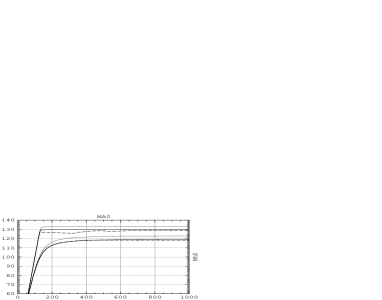
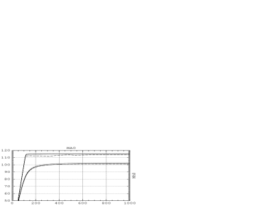
Figure 2.1: The lightest Higgs boson mass is shown as a function of $M_{A}$ in the $m_{h}^{\rm max}$ and the no-mixing scenario [53], see the Appendix. $\tan\beta$ has been set to $\tan\beta=3$ (lower curves) and $\tan\beta=50$ (upper curves). The hybrid $\overline{\rm{DR}}$/on-shell scheme (solid lines) is compared with the original on-shell (type-1) renormalization (dashed). The dotted lines indicate the effect of the “subleading” ${\cal O}(\alpha_{t}^{2})$ correction.

Two-loop ${\cal O}(\alpha_{t}^{2})$ corrections

Recently, the two-loop ${\cal O}(\alpha_{t}^{2})$ corrections in the limit of zero external momentum became available, first only for the lightest eigenvalue, $m_{h}$, and in the limit $M_{A}\gg M_{Z}$ [20], then for all the entries of the Higgs propagator matrix for arbitrary values of $M_{A}$ [21]. These corrections were obtained in the effective-potential approach, that allows to construct the Higgs boson self-energies, at zero external momenta, by taking the relevant derivatives of the field-dependent potential. In this procedure it is important, in order to make contact with the physical $M_{A}$, to compute the effective potential as a function of both ${\cal CP}$-even and ${\cal CP}$-odd fields, as emphasized in Ref. [19]. In the evaluation of the ${\cal O}(\alpha_{t}^{2})$ corrections, the specification of a renormalization prescription for the Higgs mixing parameter $\mu$ is also required and it has been chosen as $\overline{\rm{DR}}$. In FeynHiggs2.1, which includes the two-loop ${\cal O}(\alpha_{t}^{2})$ corrections, the corresponding renormalization scale is fixed to be the same as for $\delta Z_{h},\delta Z_{H}$ and $\tan\beta$.

Figure 2.2: Two-loop corrected $M_{h}$ as a function of $X_{t}$ in various steps of approximation. The relevant MSSM parameters are chosen as $\tan\beta=3\,,\,m_{t}^{\rm pole}=174.3\,\,\mathrm{GeV}$, $M_{\tilde{t}_{L}}=M_{\tilde{t}_{R}}=M_{A}=\mu=1\,\,\mathrm{TeV}$ and $m_{\tilde{g}}=800\,\,\mathrm{GeV}$. The meaning of the different curves is explained in the text.

The availability of the complete result for the momentum-independent part of the ${\cal O}(\alpha_{t}^{2})$ corrections allows to judge the quality of results that incorporate only the logarithmic contributions [14, 15]. In Fig. 2.2 (see also Fig. 2.1) we plot the two-loop corrected $m_{h}$ as a function of the stop mixing parameter, $X_{t}$. For simplicity, the soft SUSY breaking parameters in the diagonal entries of the stop mass matrix, $M_{\tilde{t}_{L}},\,M_{\tilde{t}_{R}}$, are chosen to be equal, $M_{\tilde{t}_{L}}=M_{\tilde{t}_{R}}=M_{\rm SUSY}$. For the numerical analysis $M_{\rm SUSY}$ as well as $M_{A}$ and $\mu$, are chosen to be all equal to $1\,\,\mathrm{TeV}$, while the gluino mass is $m_{\tilde{g}}=800\,\,\mathrm{GeV}$, and $\tan\beta=3$. If not otherwise stated, in all plots below we choose the trilinear couplings in the stop and sbottom sectors equal to each other, $A_{b}=A_{t}$, and set $M_{2}=M_{\rm SUSY}$, where $M_{2}$ is the SU(2) gaugino mass parameter (the U(1) gaugino mass parameter is obtained via the GUT relation, $M_{1}=5/3\,s_{\mathrm{w}}^{2}/c_{\mathrm{w}}^{2}\,M_{2}$).

The solid and dotted lines in Fig. 2.2 are computed with and without the inclusion of the full ${\cal O}(\alpha_{t}^{2})$ corrections, while the dashed and dot–dashed ones are obtained including only the logarithmic contributions. In particular, the dashed curve corresponds to the result of [14], obtained with the one-loop renormalization group method. The dot–dashed curve, instead, corresponds to the leading and next-to-leading logarithmic terms. For a more detailed discussion see Ref. [7]. From Fig. 2.2 it can also be seen that, for small $X_{t}$, the full ${\cal O}(\alpha_{t}^{2})$ result is very well reproduced by the logarithmic approximation, once the next-to-leading terms are correctly taken into account. On the other hand, when $X_{t}$ is large there are significant differences, amounting to several GeV, between the logarithmic approximation and the full result. Such differences are due to non-logarithmic terms that scale like powers of $X_{t}/M_{\rm SUSY}$. It should be noted that for more general choices of the MSSM parameters the renormalization group method becomes rather involved (see e.g. Ref. [54], where the case of a large splitting between $M_{\tilde{t}_{L}}$ and $M_{\tilde{t}_{R}}$ is discussed), and a suitable next-to-leading logarithmic approximation to the full result is much more difficult to devise.

Two-loop sbottom corrections

Due to the smallness of the bottom mass, the ${\cal O}(\alpha_{b})$ one-loop corrections to the Higgs boson self-energies can be numerically non-negligible only for $\tan\beta\gg 1$ and sizable values of the $\mu$ parameter. In fact, at the classical level $h_{b}/h_{t}=(m_{b}/m_{t})\tan\beta$, thus $\tan\beta\gg 1$ is needed in order to have $\alpha_{b}\sim\alpha_{t}$ in spite of $m_{b}\ll m_{t}$. In contrast to the ${\cal O}(\alpha_{t})$ corrections where both top and stop loops give sizable contributions, in the case of the ${\cal O}(\alpha_{b})$ corrections the numerically dominant contributions come from sbottom loops: those coming from bottom loops are always suppressed by the small value of the bottom mass. A sizable value of $\mu$ is then required to have sizable sbottom–Higgs scalar interactions in the large-$\tan\beta$ limit.

The relation between the bottom-quark mass and the Yukawa coupling $h_{b}$, which controls also the interaction between the Higgs fields and the sbottom squarks, reads at lowest order $m_{b}=h_{b}v_{1}/\sqrt{2}$. This relation is affected at one-loop order by large radiative corrections [43, 44] (see also Ref. [55]), proportional to $h_{b}v_{2}$, in general giving rise to $\tan\beta$-enhanced contributions. These terms proportional to $v_{2}$, often indicated as threshold corrections to the bottom mass, are generated either by gluino–sbottom one-loop diagrams, resulting in ${\cal O}(\alpha_{b}\alpha_{s})$ corrections to the Higgs masses, or by chargino–stop loops, giving ${\cal O}(\alpha_{b}\alpha_{t})$ corrections. Because the $\tan\beta$-enhanced contributions can be numerically relevant, an accurate determination of $h_{b}$ from the experimental value of the bottom mass requires a resummation of such effects to all orders in the perturbative expansion, as described in Ref. [44].

The leading effects are included in the effective Lagrangian formalism developed in Ref. [44]. Numerically this is by far the dominant part of the contributions from the sbottom sector. The effective Lagrangian is given by

$${\cal L}=\frac{g}{2M_{W}}\frac{\overline{m}_{b}}{1+\Delta m_{b}}\Bigg{[} \tan\beta\;A\,i\,\bar{b}\gamma_{5}b+\sqrt{2}\,V_{tb}\,\tan\beta\;H^{+}\bar{t}_{L}b_{R}$$ (2.108)

$$+ \left(\frac{\sin\alpha\hskip 2.84526pt}{\cos\beta\hskip 2.84526pt}-\Delta m_{b}\frac{\cos\alpha\hskip 2.84526pt}{\sin\beta}\right)h\bar{b}_{L}b_{R}$$

$$- \left(\frac{\cos\alpha\hskip 2.84526pt}{\cos\beta\hskip 2.84526pt}+\Delta m_{b}\frac{\sin\alpha\hskip 2.84526pt}{\sin\beta}\right)H\bar{b}_{L}b_{R}\Bigg{]}+{\rm h.c.}~{}.$$

Here $\overline{m}_{b}$ denotes the running bottom quark mass including SM QCD corrections. In the numerical evaluations we choose $\overline{m}_{b}=\overline{m}_{b}(m_{t})\approx 2.74\,\,\mathrm{GeV}$. Furthermore, $\Delta m_{b}$ is given at ${\cal O}(\alpha_{s})$ by

$$\Delta m_{b}=\frac{2\alpha_{s}}{3\,\pi}\,m_{\tilde{g}}\,\mu\,\tan\beta\,\times\,I(m_{\tilde{b}_{1}},m_{\tilde{b}_{2}},m_{\tilde{g}}),$$ (2.109)

where $I$ is given by

$$I(a,b,c)=\frac{1}{(a^{2}-b^{2})(b^{2}-c^{2})(a^{2}-c^{2})}\,\left(a^{2}b^{2}\log\frac{a^{2}}{b^{2}}+b^{2}c^{2}\log\frac{b^{2}}{c^{2}}+c^{2}a^{2}\log\frac{c^{2}}{a^{2}}\right).$$ (2.110)

The large $\tilde{b}-\tilde{g}$ loops are resummed to all orders of $(\alpha_{s}\tan\beta)^{n}$ via the inclusion of $\Delta m_{b}$ [44]. The prefactor $1/(1+\Delta m_{b})$ in eq. (2.108) arises from the resummation of the leading corrections to all orders. They are due to the shift in the relation of the bottom Yukawa coupling to the physical $b$ quark mass, coming from the loop induced coupling of the $\phi_{1}$ to the bottom quarks. The additional terms $\sim\Delta m_{b}$ in the $h\bar{b}b$ and $H\bar{b}b$ couplings arise from the mixing and coupling of the “other” Higgs boson, $H$ and $h$, respectively, to the $b$ quarks.

The $b/\tilde{b}$ corrections to the renormalized Higgs boson self-energies in eq. (2.81) are given at the one-loop level by the Feynman diagrams shown in Figs. 2.3, 2.4.

Figure 2.3: Generic Feynman diagrams for the $b/\tilde{b}$ contributions to Higgs boson self-energies (H = $h,H,A$).

                 

Figure 2.4: Generic Feynman diagrams for the $b/\tilde{b}$ contributions to Higgs tadpoles (H = $h,H$).

The $\Delta m_{b}$ corrections included in the effective Lagrangian, eq. (2.108), enter the one-loop diagrams in the following ways:

• The factor $(m_{b}\sin\alpha\hskip 2.84526pt/\cos\beta\hskip 2.84526pt)$ in the $hb\bar{b}$ coupling changes to

  $$m_{b}\frac{\sin\alpha\hskip 2.84526pt}{\cos\beta\hskip 2.84526pt}\to\frac{m_{b}}{1+\Delta m_{b}}\left(\frac{\sin\alpha\hskip 2.84526pt}{\cos\beta\hskip 2.84526pt}-\Delta m_{b}\frac{\cos\alpha\hskip 2.84526pt}{\sin\beta}\right).$$ (2.111)

  The corresponding factor $(-m_{b}\cos\alpha\hskip 2.84526pt/\cos\beta\hskip 2.84526pt)$ in the $Hb\bar{b}$ coupling is shifted to

  $$-m_{b}\frac{\cos\alpha\hskip 2.84526pt}{\cos\beta\hskip 2.84526pt}\to-\frac{m_{b}}{1+\Delta m_{b}}\left(\frac{\cos\alpha\hskip 2.84526pt}{\cos\beta\hskip 2.84526pt}+\Delta m_{b}\frac{\sin\alpha\hskip 2.84526pt}{\sin\beta}\right).$$ (2.112)

  Finally, the $Ab\bar{b}$ coupling receives the factor

  $$m_{b}\to\frac{m_{b}}{1+\Delta m_{b}}.$$ (2.113)

  It should be noted that the $b$ quark masses appearing in the bottom propagators do not receive a correction.

• The $b$ quark masses in the $\tilde{b}$ mass matrix (2.63) are due to Yukawa couplings from the scalar bottoms to the Higgs doublets. Thus they receive the shift

  $$m_{b}\to\frac{m_{b}}{1+\Delta m_{b}}.$$ (2.114)

• For the same reason the $m_{b}$ factors in the Higgs-$\tilde{b}\bar{\tilde{b}}$ couplings receive the same shift as given in eq. (2.114).

Using the above changes in the one-loop corrections includes the leading $b/\tilde{b}$ corrections beyond one-loop, resummed to all orders.

Recently the complete two-loop  momentum-independent, ${\cal O}(\alpha_{b}\alpha_{s})$ corrections (which are not included in the ${\cal O}(\alpha_{b}(\alpha_{s}\tan\beta)^{n})$ resummation) have been computed [22, 23]. The result obtained makes use of an appropriate choice of renormalization conditions on the relevant parameters that allows to disentangle the genuine two-loop effects from the large threshold corrections to the bottom mass, and also ensures the decoupling of heavy gluinos.

Figure 2.5: The result for the lightest ${\cal CP}$-even Higgs-boson mass in the MSSM, $M_{h}$, as obtained with the program FeynHiggs is shown as a function of $\tan\beta$ for $M_{A}=120$ GeV, $\mu=-1\,\,\mathrm{TeV}$, $M_{\tilde{t}_{L}}=M_{\tilde{t}_{R}}=M_{\tilde{b}_{R}}=m_{\tilde{g}}=1$ TeV, $A_{t}=A_{b}=2\,\,\mathrm{TeV}$. The meaning of the different curves is explained in the text.

To appreciate the importance of the various sbottom contributions, we plot in Fig. 2.5 the light Higgs mass $M_{h}$ as a function of $\tan\beta$. The SM running bottom mass computed at the top mass scale, $m_{b}(m_{t})=2.74$ GeV, is used in order to account for the universal large QCD corrections. The relevant MSSM parameters are chosen as $M_{A}=120\,\,\mathrm{GeV}$, $\mu=-1\,\,\mathrm{TeV}$, $M_{\tilde{t}_{L}}=M_{\tilde{t}_{R}}=M_{\tilde{b}_{R}}=m_{\tilde{g}}=1\,\,\mathrm{TeV}$, $A_{t}=A_{b}=2\,\,\mathrm{TeV}$. The dot–dashed curve in Fig. 2.5 includes the full one-loop contribution as well as the two-loop ${\cal O}(\alpha_{t}\alpha_{s}+\alpha_{t}^{2})$ corrections (the latter being approximately $\tan\beta$-independent when $\tan\beta$ is large). The dashed curve includes also the resummation of the $\tan\beta$-enhanced threshold effects in the relation between $h_{b}$ and $m_{b}$. Finally, the solid curve includes in addition the complete ${\cal O}(\alpha_{b}\alpha_{s})$ two-loop corrections of Ref. [22]. In the last two curves, the steep dependence of $m_{h}$ on $\tan\beta$ when the latter is large is driven by the sbottom contributions. One sees that the $\tan\beta$-enhanced threshold effects account for the bulk of the sbottom contributions beyond one-loop. The genuine ${\cal O}(\alpha_{b}\alpha_{s})$ two-loop corrections can still shift $m_{h}$ by a few GeV for very large values of $\tan\beta$ and $\mu$.

2.3.5 Implications for $\tan\beta$ exclusion bounds

The improved knowledge of the two-loop contributions to the Higgs boson self-energies results in a very precise prediction for the Higgs boson masses and mixing angle with interesting implications for MSSM parameter space analyses. In this section an important consequence of the various corrections is presented: the implications on the upper limit on $m_{h}$ within the MSSM and on the corresponding limit on $\tan\beta$ arising from confronting the upper bound on $m_{h}$ with the lower limit from Higgs searches, see also the discussion in Ref. [6].

The theoretical upper bound on the lightest Higgs boson mass as a function of $\tan\beta$ can be combined with the results from direct searches at LEP to constrain $\tan\beta$. The diagonalization of the tree-level mass matrix, eq. (2.40), yields a value for $m_{h,{\rm tree}}$ that is maximal when $M_{A}\gg M_{Z}$, in which case $m_{h,{\rm tree}}^{2}\simeq M_{Z}^{2}\,\cos^{2}2\beta\hskip 2.84526pt$, which vanishes for $\tan\beta=1$. Radiative corrections significantly increase the light Higgs boson mass compared to its tree-level value, but still $m_{h}$ is minimized for values of $\tan\beta$ around one. Thus, in principle, the region of low $\tan\beta$ can be probed experimentally via the search for the lightest MSSM Higgs boson [56]. If the remaining MSSM parameters are tuned in such a way to obtain the maximal value of $M_{h}$ as a function of $\tan\beta$ (for reasonable values of $M_{\rm SUSY}$ and taking into account the experimental uncertainties of $m_{t}$ and the other SM input parameters as well as the theoretical uncertainties from unknown higher-order corrections), the experimental lower bound on $M_{h}$ can be used to obtain exclusion limits for $\tan\beta$. While in general a detailed investigation of a variety of different possible production and decay modes is necessary in order to determine whether a particular point of the MSSM parameter space can be excluded via the Higgs searches or not, the situation simplifies considerably in the region of small $\tan\beta$ values. In this parameter region the lightest ${\cal CP}$-even Higgs boson of the MSSM couples to the $Z$ boson with SM-like strength, and its decay into a $b\bar{b}$ pair is not significantly suppressed. Thus, within good approximation, constraints on $\tan\beta$ can be obtained in this parameter region by confronting the exclusion bound on the SM Higgs boson with the upper limit on $M_{h}$ within the MSSM. We use this approach below in order to discuss the implications of the new $M_{h}$ evaluation on $\tan\beta$ exclusion bounds.

Concerning the upper bound on $M_{h}$ within the MSSM, the one-loop corrections contribute positively to $M_{h}^{2}$. The two-loop effects of ${\cal O}(\alpha_{t}\alpha_{s})$ and ${\cal O}(\alpha_{t}^{2})$, on the other hand, enter with competing signs, the former reducing $M_{h}^{2}$ while the latter give a (smaller) positive contribution. The actual bound that can be derived depends sensitively on the precise value of the top-quark mass, because the dominant one-loop contribution to $M_{h}^{2}$, as well as the two-loop ${\cal O}(\alpha_{t}\alpha_{s})$ term, scale as $m_{t}^{4}$. Furthermore, a large top mass amplifies the relative importance of the two-loop ${\cal O}(\alpha_{t}^{2})$ correction, because of the additional $m_{t}^{2}$ factor.

In order to discuss restrictions on the MSSM parameter space it has become customary in the recent years to refer to so-called benchmark scenarios of MSSM parameters [53, 57]. The $m_{h}^{\rm max}$ benchmark scenario [53] has been designed such that for fixed values of $m_{t}$ and $M_{\rm SUSY}$ the predicted value of the lightest ${\cal CP}$-even Higgs boson mass is maximized for each value of $M_{A}$ and $\tan\beta$. The value of the top-quark mass had been fixed to its experimental central value, $m_{t}=174.3\,\,\mathrm{GeV}$, while the SUSY parameters are taken as in the $m_{h}^{\rm max}$ scenario, see the Appendix. Furthermore, $M_{A}$ has been fixed to $M_{A}=1\,\,\mathrm{TeV}$.

Figure 2.6: The result for the lightest ${\cal CP}$-even Higgs boson mass, $M_{h}$, as a function of $\tan\beta$ in the $m_{h}^{\rm max}$ scenario. The dotted curve has been obtained with a renormalization-group improved effective potential method, using the code subhpoledm. The short-dashed curve corresponds to the result obtained with FeynHiggs1.0, while the dash-dotted curve shows the result of FeynHiggs1.3, where the improvements described in Sect. 2.3.4 are included. The full curve shows the result from FeynHiggs2.1, using the top quark mass of $m_{t}=178.0\,\,\mathrm{GeV}$. The dot-dashed curve, also obtained with FeynHiggs2.1, employs $m_{t}=182.3\,\,\mathrm{GeV}$ and $M_{\rm SUSY}=2\,\,\mathrm{TeV}$. The vertical long-dashed line corresponds to the LEP exclusion bound for the SM Higgs boson of $114.4\,\,\mathrm{GeV}$.

In Fig. 2.6 we plot $M_{h}$ as a function of $\tan\beta$ in the $m_{h}^{\rm max}$ scenario. The dashed and dot-dashed curves correspond to the result obtained with the previous (used for the LEP evaluations so far [56]) and the more advanced version (where the improvements described in Sect. 2.3.4 are included, and which will be used for the final LEP evaluations [58]) of FeynHiggs, respectively. The two versions, FeynHiggs1.0 and FeynHiggs1.3, differ by the recent improvements obtained in the MSSM Higgs sector which are described in Sect. 2.3.4. Also shown as a solid line is the result obtained with FeynHiggs2.1 (which for the $m_{h}^{\rm max}$ scenario should yield quantitatively the same result as FeynHiggs1.3), but with $m_{t}$ set to the recently obtained new experimental value, $m_{t}^{\rm exp}=178.0\,\,\mathrm{GeV}$ [3]. For comparison, also the result obtained with a renormalization-group improved effective potential method is indicated. The dotted curve in Fig. 2.6 corresponds to the code subhpoledm [14, 59, 44] in the $m_{h}^{\rm max}$ scenario, for a $\tilde{t}$ mixing parameter $X_{t}^{\overline{\rm{MS}}}=\sqrt{6}\,M_{\rm SUSY}$ [14, 59] (see also the Appendix). It deviates from the result of FeynHiggs1.0 by typically not more than 1 GeV for $\tan\beta\geq 1$. The LEP exclusion bound for the mass of a SM-like Higgs [60], $M_{H_{\rm SM}}\geq 114.4\,\,\mathrm{GeV}$, is shown in the figure as a vertical long–dashed line. As can be seen from the figure, the improvements on the theoretical prediction described in Sect. 2.3.4, in particular the inclusion of the complete momentum-independent ${\cal O}(\alpha_{t}^{2})$ corrections into FeynHiggs, gives rise to a significant increase in the upper bound on $M_{h}$ as a function of $\tan\beta$. Comparison of this prediction with the exclusion bound on a SM-like Higgs shows that the lower limit on $\tan\beta$ is considerably weakened. Also the new top mass value, see the solid line, shifting the resulting $M_{h}$ values upwards, weakens the $\tan\beta$ exclusion bound.

Concerning the interpretation of the results shown in Fig. 2.6, it should be kept in mind that within the (pure) $m_{h}^{\rm max}$ benchmark scenario $m_{t}$ and $M_{\rm SUSY}$ are kept fixed, and no theoretical uncertainties from unknown higher-order corrections are taken into account. In order to arrive at a more general exclusion bound on $\tan\beta$ that is not restricted to a particular benchmark scenario, the impact of the parametric and higher-order uncertainties in the prediction for $M_{h}$ has to be considered [6]. In order to demonstrate in particular the dependence of the $\tan\beta$ exclusion bound on the chosen value of the top pole mass, besides the solid line obtained with $m_{t}=178.0\,\,\mathrm{GeV}$, the dot–dashed curve in Fig. 2.6 shows the result obtained with FeynHiggs2.1 where the top-quark mass has been increased by one standard deviation, $\sigma_{m_{t}}=4.3\,\,\,\mathrm{GeV}$, to $m_{t}=182.3\,\,\mathrm{GeV}$, and $M_{\rm SUSY}$ has been changed from 1 TeV to 2 TeV. It can be seen that in this more general scenario no lower limit on $\tan\beta$ from the LEP Higgs searches can be obtained.

Constraints from the Higgs searches at LEP do of course play an important role in regions of the MSSM parameter space where the parameters are such that $M_{h}$ does not reach its maximum value. Also in this case, however, the remaining theoretical uncertainties from unknown higher-order corrections (see Sect. 2.5 below) have to be taken into account in order to obtain conservative exclusion limits.

2.4 Comparison with the RG approach

The diagrammatic two-loop computation of the dominant contributions at ${\cal O}(\alpha\alpha_{s})$ to the neutral ${\cal CP}$-even Higgs boson masses [16] had been obtained first in the on-shell scheme, was subsequently combined [5] with the complete diagrammatic one-loop on-shell result of Ref. [11]. Within the RG approach [14, 15], on the other hand, the two-loop results was expressed in terms of the top-quark mass in the $\overline{\rm{MS}}$ scheme.

Besides a sizable shift in the upper bound of $M_{h}$ of about $5\,\,\mathrm{GeV}$, apparent deviations between the explicit diagrammatic two-loop calculation and the results of the RG computation were observed in the dependence of $M_{h}$ on the stop-mixing parameter $X_{t}$. While the value of $X_{t}$ that maximizes the lightest ${\cal CP}$-even Higgs mass is $(X_{t})_{\rm max}\simeq\pm\sqrt{6}\,M_{S}\approx\pm 2.4\,M_{S}$ ($M_{S}$ denotes the soft SUSY-breaking parameter in the $\tilde{t}$ and $\tilde{b}$ sector, $M_{S}\equiv M_{\tilde{t}_{L}}=M_{\tilde{t}_{R}}=M_{\tilde{b}_{L}}=M_{\tilde{b}_{R}}$) in the RG results, the corresponding on-shell two-loop diagrammatic computation found a maximal value for $M_{h}$ at $(X_{t})_{\rm max}\approx 2M_{S}$. Moreover, the RG result is symmetric under $X_{t}\to-X_{t}$ and has a (local) minimum at $X_{t}=0$. In contrast, the two-loop diagrammatic computation yields $M_{h}$ values for positive and negative $X_{t}$ that differ significantly from each other and the local minimum in $M_{h}$ is shifted slightly away from $X_{t}=0$ [17].

In this section, it is shown that this apparent discrepancy is caused by the different renormalization schemes employed in the two approaches, leading to differences in the leading-logarithmic contributions. It will furthermore be shown that in the analytic approximation for the leading $m_{t}^{4}$ corrections, the dominant numerical contribution of the new genuine non-logarithmic two-loop contributions of the FD result [16, 5] can be absorbed into an effective one-loop expression by choosing an appropriate scale for the running top-quark mass in different terms of the expression.

2.4.1 Approximation formulas for $M_{h}$

Within the RG approach the following approximation for $M_{h}$ has been obtained [13, 14, 15, 59], taking into account terms up to ${\cal O}(\alpha\alpha_{s})$:

$$M_{h}^{2}=m_{h}^{2,{\rm tree}}+\frac{3}{2}\frac{G_{F}\sqrt{2}}{\pi^{2}}\overline{m}_{t}^{4}\left\{-\ln\left(\frac{\overline{m}_{t}^{2}}{\overline{M}_{S}^{\lower 2.0pt\hbox{$\scriptstyle\,2$}}}\right)+\frac{\overline{X}_{t}^{\lower 2.0pt\hbox{$\scriptstyle\,2$}}}{\overline{M}_{S}^{\lower 2.0pt\hbox{$\scriptstyle\,2$}}}\left(1-\frac{1}{12}\frac{\overline{X}_{t}^{\lower 2.0pt\hbox{$\scriptstyle\,2$}}}{\overline{M}_{S}^{\lower 2.0pt\hbox{$\scriptstyle\,2$}}}\right)\right\}$$ (2.115)

$${}-3\frac{G_{F}\sqrt{2}}{\pi^{2}}\frac{\alpha_{s}}{\pi}\overline{m}_{t}^{4}\left\{\ln^{2}\left(\frac{\overline{m}_{t}^{2}}{\overline{M}_{S}^{\lower 2.0pt\hbox{$\scriptstyle\,2$}}}\right)+\left[\frac{2}{3}-2\frac{\overline{X}_{t}^{\lower 2.0pt\hbox{$\scriptstyle\,2$}}}{\overline{M}_{S}^{\lower 2.0pt\hbox{$\scriptstyle\,2$}}}\left(1-\frac{1}{12}\frac{\overline{X}_{t}^{\lower 2.0pt\hbox{$\scriptstyle\,2$}}}{\overline{M}_{S}^{\lower 2.0pt\hbox{$\scriptstyle\,2$}}}\right)\right]\ln\left(\frac{\overline{m}_{t}^{2}}{\overline{M}_{S}^{\lower 2.0pt\hbox{$\scriptstyle\,2$}}}\right)\right\},$$

where we have introduced the notation $\overline{M}_{S},\overline{X}_{t}$ to emphasize that the corresponding quantities are $\overline{\rm{MS}}$ parameters, which are evaluated at the scale $\mu=M_{S}$:

$$\overline{M}_{S}\equiv M_{S}^{\overline{\mathrm{MS}}}(M_{S}),\quad\overline{X}_{t}\equiv X_{t}^{\overline{\mathrm{MS}}}(M_{S}),$$ (2.116)

and $\overline{m}_{t}\equiv m^{\overline{\mathrm{MS}}}_{t,\mathrm{SM}}(m_{t})$ is the $\overline{\rm{MS}}$ top mass

$$\overline{m}_{t}=\overline{m}_{t}(m_{t})\approx\frac{M_{t}}{1+\frac{4}{3\,\pi}\alpha_{s}(m_{t})}~{}.$$ (2.117)

$M_{t}$ denotes the top quark pole mass. Since in this section only the ${\cal O}(\alpha\alpha_{s})$ corrections are investigated, we do not include here the contributions of ${\cal O}(\alpha_{t})$, see however Sect. 2.5.4.

Concerning the FD result, we consider the dominant one-loop and two-loop terms and we focus on the case $M_{A}\gg M_{Z}$, for which the result for $M_{h}^{2}$ can be expressed in a particularly compact form [17]

$$M_{h}^{2}=m_{h}^{2,{\rm tree}}+m_{h}^{2,{\alpha}}+m_{h}^{2,{\alpha\alpha_{s}}},$$ (2.118)

and neglect the non-leading terms of ${\cal O}(M_{Z}^{2}/M_{A}^{2})$. Assuming that $M_{S}\gg M_{t}$ and neglecting the non-leading terms of ${\cal O}(M_{t}/M_{S})$ and ${\cal O}(M_{Z}^{2}/M_{t}^{2})$, one obtains the following simple result for the one-loop and two-loop contributions

$$m_{h}^{2,{\alpha}} = \frac{3}{2}\frac{G_{F}\sqrt{2}}{\pi^{2}}M_{t}^{4}\left\{-\ln\left(\frac{M_{t}^{2}}{M_{S}^{2}}\right)+\frac{X_{t}^{2}}{M_{S}^{2}}\left(1-\frac{1}{12}\frac{X_{t}^{2}}{M_{S}^{2}}\right)\right\},$$ (2.119)

$$m_{h}^{2,{\alpha\alpha_{s}}} = -3\frac{G_{F}\sqrt{2}}{\pi^{2}}\frac{\alpha_{s}}{\pi}M_{t}^{4}\left\{\ln^{2}\left(\frac{M_{t}^{2}}{M_{S}^{2}}\right)-\left(2+\frac{X_{t}^{2}}{M_{S}^{2}}\right)\ln\left(\frac{M_{t}^{2}}{M_{S}^{2}}\right)-\frac{X_{t}}{M_{S}}\left(2-\frac{1}{4}\frac{X_{t}^{3}}{M_{S}^{3}}\right)\right\}.$$

The corresponding formulae, in which terms up to ${\cal O}(M_{t}^{4}/M_{S}^{4})$ are kept, can be found in Ref. [59].

In eqs. (2.119)-(LABEL:eq:mh2ldiagos) the parameters $M_{t}$, $M_{S}$, $X_{t}$ are on-shell quantities. Using eq. (2.117), the on-shell result for $M_{h}^{2}$, eqs. (2.118)–(LABEL:eq:mh2ldiagos), can easily be rewritten in terms of the running top-quark mass $\overline{m}_{t}$. While this reparameterization does not change the form of the one-loop result, it induces an extra contribution at ${\cal O}(\alpha\alpha_{s})$. Keeping again only terms that are not suppressed by powers of $\overline{m}_{t}/M_{S}$, the resulting expressions read

$$m_{h}^{2,{\alpha}} = \frac{3}{2}\frac{G_{F}\sqrt{2}}{\pi^{2}}\overline{m}_{t}^{4}\Biggl{\{}-\ln\left(\frac{\overline{m}_{t}^{2}}{M_{S}^{2}}\right)+\frac{X_{t}^{2}}{M_{S}^{2}}\left(1-\frac{1}{12}\frac{X_{t}^{2}}{M_{S}^{2}}\right)\Biggr{\}},$$ (2.121)

$$m_{h}^{2,{\alpha\alpha_{s}}} = -3\frac{G_{F}\sqrt{2}}{\pi^{2}}\frac{\alpha_{s}}{\pi}\overline{m}_{t}^{4}\Biggl{\{}\ln^{2}\left(\frac{\overline{m}_{t}^{2}}{M_{S}^{2}}\right)+\left(\frac{2}{3}-\frac{X_{t}^{2}}{M_{S}^{2}}\right)\ln\left(\frac{\overline{m}_{t}^{2}}{M_{S}^{2}}\right)$$ (2.122)

$${}+\frac{4}{3}-2\frac{X_{t}}{M_{S}}-\frac{8}{3}\frac{X_{t}^{2}}{M_{S}^{2}}+\frac{17}{36}\frac{X_{t}^{4}}{M_{S}^{4}}\Biggr{\}},$$

in accordance with the formulae given in Ref. [17].

We now compare the diagrammatic result expressed in terms of the parameters $\overline{m}_{t}$, $M_{S}$, $X_{t}$, eqs. (2.121)-(2.122), with the RG result of eq. (2.115), which is given in terms of the $\overline{\rm{MS}}$ parameters $\overline{m}_{t}$, $\overline{M}_{S}$, $\overline{X}_{t}$ eq. (2.116). While the $X_{t}$-independent logarithmic terms are the same in both the diagrammatic and RG results, the corresponding logarithmic terms at two loops that are proportional to powers of $X_{t}$ and $\overline{X}_{t}$, respectively, are different. Furthermore, eq. (2.122) does not contain a logarithmic term proportional to $X_{t}^{4}$, while the corresponding term proportional to $\overline{X}_{t}^{\lower 2.0pt\hbox{$\scriptstyle\,4$}}$ appears in eq. (2.115). To check whether these results are consistent with each other, one must relate the on-shell and $\overline{\rm{MS}}$ definitions of the parameters $M_{S}$ and $X_{t}$.

Finally, we note that the non-logarithmic terms contained in eq. (2.122) correspond to genuine two-loop contributions that are not present in the RG result of eq. (2.115). They can be interpreted as a two-loop finite threshold correction to the quartic Higgs self-coupling in the RG approach. In particular, note that eq. (2.122) contains a term that is linear in $X_{t}$. This is the main source of the asymmetry in the two-loop corrected Higgs mass under $X_{t}\to-X_{t}$ obtained by the diagrammatic method. The non-logarithmic terms in eq. (2.122) give rise to a numerically significant increase of the maximal value of $M_{h}$ of about 5 GeV in this approximation.

2.4.2 On-shell and $\overline{\rm MS}$ definitions of $M_{S}$ and $X_{t}$

Since the parameters $p=\{m_{\tilde{t}_{1}}^{2},m_{\tilde{t}_{2}}^{2},\theta_{\tilde{t}},m_{t}\}$ of the $t$–$\tilde{t}$ sector are renormalized differently in different schemes, the parameters $M_{S}$ and $X_{t}$ also have a different meaning in these schemes. The relation between these parameters in the $\overline{\rm{MS}}$ and in the on-shell scheme have been derived in Refs. [59, 61] and read in leading order in $m_{t}/M_{S}$:

$$\overline{M}_{S}^{\lower 2.0pt\hbox{$\scriptstyle\,2$}} = M_{S}^{2,\mathrm{OS}}-\frac{8}{3}\frac{\alpha_{s}}{\pi}M_{S}^{2}\,,$$ (2.123)

$$\overline{X}_{t} = X_{t}^{\mathrm{OS}}\frac{M_{t}}{\overline{m}_{t}(M_{S})}+\frac{8}{3}\frac{\alpha_{s}}{\pi}M_{S}\,.$$ (2.124)

As previously noted, it is not necessary to specify the definition of the parameters that appear in the ${\cal O}(\alpha_{s})$ terms as long as higher orders are neglected. Thus, we use the generic symbol $M_{S}^{2}$ in the ${\cal O}(\alpha_{s})$ terms of eqs. (2.123)–(2.124). The corresponding results including terms up to ${\cal O}\left(m_{t}^{4}/M_{S}^{4}\right)$ can be found in Ref. [59].

Finally, the evaluation of the ratio $M_{t}/\overline{m}_{t}(M_{S})$ is needed. In leading order in $m_{t}/M_{S}$ it is given by [59]:

$$\overline{m}_{t}(M_{S})=\overline{m}_{t}\left[1+\frac{\alpha_{s}}{\pi}\ln\left(\frac{m_{t}^{2}}{M_{S}^{2}}\right)+\frac{\alpha_{s}}{3\pi}\frac{X_{t}}{M_{S}}\right]\,,$$ (2.125)

where $\overline{m}_{t}\equiv m^{\overline{\mathrm{MS}}}_{t,\mathrm{SM}}(m_{t})$ is given in terms of $M_{t}$ by eq. (2.117). Note that the term in eq. (2.125) that is proportional to $X_{t}$ is a threshold correction due to the supersymmetry-breaking stop-mixing effect. Inserting the result of eq. (2.125) into eq. (2.124) yields

$$\overline{X}_{t}=X_{t}^{\mathrm{OS}}+\frac{\alpha_{s}}{3\pi}M_{S}\left[8+\frac{4X_{t}}{M_{S}}-\frac{X_{t}^{2}}{M_{S}^{2}}-\frac{3X_{t}}{M_{S}}\ln\left(\frac{m_{t}^{2}}{M_{S}^{2}}\right)\right]\,.$$ (2.126)

It is interesting to note that $\overline{X}_{t}\neq 0$ when $X_{t}^{\mathrm{OS}}=0$. Moreover, it is clear from eq. (2.126) that the relation between $X_{t}$ defined in the on-shell and the $\overline{\rm{MS}}$ schemes includes a leading logarithmic effect, which has to be taken into account in a comparison of the leading logarithmic contributions in the RG and the two-loop diagrammatic results.

A remark on the regularization scheme is in order here. In the effective field theory, the running top-quark mass at scales below $M_{S}$ is the SM running coupling of eq. (2.117), which is calculated in dimensional regularization. This is matched to the running top-quark mass as computed in the full supersymmetric theory. One could argue that the appropriate regularization scheme for the latter should be dimensional reduction (DRED) [50], which is usually applied in loop calculations in supersymmetry. The result of such a change would be to modify slightly the two-loop non-logarithmic contribution to $M_{h}$ that is proportional to powers of $X_{t}$. Of course, the physical Higgs mass is independent of any scheme. One is free to re-express eqs. (2.119)-(LABEL:eq:mh2ldiagos) (which depend on the on-shell parameters $M_{t}$, $M_{S}$, $X_{t}$) in terms of parameters defined in any other scheme. In this paper, we find $\overline{\rm{MS}}$–renormalization via DREG to be the most convenient scheme for the comparison of the diagrammatic and RG results for $M_{h}$.

2.4.3 Comparing the RG and the Feynman diagrammatic results

In order to directly compare the two-loop diagrammatic and RG results, we must convert from on-shell to $\overline{\rm{MS}}$ parameters. Inserting eqs. (2.123)-(2.126) into eqs. (2.121)-(2.122), one finds

$$m_{h}^{2,{\alpha}} = \frac{3}{2}\frac{G_{F}\sqrt{2}}{\pi^{2}}\overline{m}_{t}^{4}\left\{-\ln\left(\frac{\overline{m}_{t}^{2}}{\overline{M}_{S}^{\lower 2.0pt\hbox{$\scriptstyle\,2$}}}\right)+\frac{\overline{X}_{t}^{\lower 2.0pt\hbox{$\scriptstyle\,2$}}}{\overline{M}_{S}^{\lower 2.0pt\hbox{$\scriptstyle\,2$}}}\left(1-\frac{1}{12}\frac{\overline{X}_{t}^{\lower 2.0pt\hbox{$\scriptstyle\,2$}}}{\overline{M}_{S}^{\lower 2.0pt\hbox{$\scriptstyle\,2$}}}\right)\right\}\,,$$ (2.127)

$$m_{h}^{2,{\alpha\alpha_{s}}} = -3\frac{G_{F}\sqrt{2}}{\pi^{2}}\frac{\alpha_{s}}{\pi}\overline{m}_{t}^{4}\Biggl{\{}\ln^{2}\left(\frac{\overline{m}_{t}^{2}}{\overline{M}_{S}^{\lower 2.0pt\hbox{$\scriptstyle\,2$}}}\right)+\left[\frac{2}{3}-2\frac{\overline{X}_{t}^{\lower 2.0pt\hbox{$\scriptstyle\,2$}}}{\overline{M}_{S}^{\lower 2.0pt\hbox{$\scriptstyle\,2$}}}\left(1-\frac{1}{12}\frac{\overline{X}_{t}^{\lower 2.0pt\hbox{$\scriptstyle\,2$}}}{\overline{M}_{S}^{\lower 2.0pt\hbox{$\scriptstyle\,2$}}}\right)\right]\ln\left(\frac{\overline{m}_{t}^{2}}{\overline{M}_{S}^{\lower 2.0pt\hbox{$\scriptstyle\,2$}}}\right)$$ (2.128)

$${}+\frac{\overline{X}_{t}}{\overline{M}_{S}}\left(\frac{2}{3}-\frac{7}{9}\frac{\overline{X}_{t}^{\lower 2.0pt\hbox{$\scriptstyle\,2$}}}{\overline{M}_{S}^{\lower 2.0pt\hbox{$\scriptstyle\,2$}}}+\frac{1}{36}\frac{\overline{X}_{t}^{\lower 2.0pt\hbox{$\scriptstyle\,3$}}}{\overline{M}_{S}^{\lower 2.0pt\hbox{$\scriptstyle\,3$}}}+\frac{1}{18}\frac{\overline{X}_{t}^{\lower 2.0pt\hbox{$\scriptstyle\,4$}}}{\overline{M}_{S}^{\lower 2.0pt\hbox{$\scriptstyle\,4$}}}\right)\Biggr{\}}+{\cal O}\left(\frac{\overline{m}_{t}}{\overline{M}_{S}}\right)\,.$$

Comparing eq. (2.128) with eq. (2.115) shows that the logarithmic contributions of the diagrammatic result expressed in terms of the $\overline{\rm{MS}}$ parameters $\overline{m}_{t}$, $\overline{M}_{S}$, $\overline{X}_{t}$ agree with the logarithmic contributions obtained by the RG approach. The differences in the logarithmic terms observed in the comparison of eqs. (2.121)-(2.122) with eq. (2.115) have thus been traced to the different renormalization schemes applied in the respective calculations. The fact that the logarithmic contributions obtained within the two approaches agree after a proper rewriting of the parameters of the stop sector is an important consistency check of the calculations. In addition to the logarithmic contributions, eq. (2.128) also contains non-logarithmic contributions, which are numerically sizable.

Figure 2.7: Comparison of the diagrammatic two-loop ${\cal O}(\alpha\alpha_{s})$ result for $M_{h}$, to leading order in $\overline{m}_{t}/\overline{M}_{S}$ (eqs. (2.127)-(2.128)) with the RG result of eq. (2.115). Note that the latter omits the one-loop threshold corrections due to stop mixing in the evaluation of $\overline{m}_{t}(M_{S})$. Since this quantity enters in the definition of $\overline{X}_{t}$, see eq. (2.124), the meaning of $X_{t}^{\rm MS}$ plotted along the $x$-axis is slightly different for the diagrammatic curve, where $X_{t}^{\rm MS}=\overline{X}_{t}$, and the RG curve, where $X_{t}^{\rm MS}=\overline{X}_{t}\,[1+(\alpha_{s}/3\pi)(X_{t}/M_{S})]$. See text for further details. The graph is plotted for $\overline{M}_{S}=M_{A}=(m_{\tilde{g}}^{2}+\overline{m}_{t}^{2})^{1/2}=1\,\,\mathrm{TeV}$.

In Fig. 2.7, we compare the diagrammatic result for $M_{h}$ in the leading $m_{t}^{4}$ approximation to the results obtained by RG techniques. While the diagrammatic result expressed in terms of $\overline{m}_{t}$, $\overline{M}_{S}$, $\overline{X}_{t}$ agrees well with the RG result in the region of no mixing in the stop sector, sizable deviations occur for large mixing. In particular, the non-logarithmic contributions give rise to an asymmetry under the change of sign of the parameter $\overline{X}_{t}$, while the RG result is symmetric under $\overline{X}_{t}\to-\overline{X}_{t}$. In the approximation considered here, the maximal value for $M_{h}$ in the diagrammatic result lies about 3 GeV higher than the maximal value of the RG result. The differences are slightly larger for smaller $\tan\beta$ values. In addition, as previously noted, the maximal-mixing point $(\overline{X}_{t})_{\rm max}$ (where the radiatively corrected value of $M_{h}$ is maximal) is equal to its one-loop value, $(\overline{X}_{t})_{\rm max}\simeq\pm\sqrt{6}M_{S}$, in the RG result of eq. (2.115), while it is shifted in the two-loop diagrammatic result. However, Fig. 2.7 illustrates that the shift in $(\overline{X}_{t})_{\rm max}$ from its one-loop value, while significant in the two-loop on-shell diagrammatic result, is largely diminished when the latter is re-expressed in terms of $\overline{\rm{MS}}$ parameters.

The differences between the diagrammatic and RG results shown in Fig. 2.7 can be attributed to non-negligible non-logarithmic terms proportional to powers of $X_{t}$. Clearly, the RG technique can be improved to incorporate these terms. In Ref. [15], it was shown that the leading two-loop contributions to $M_{h}^{2}$ given by the RG result of eq. (2.115) could be absorbed into an effective one-loop expression. This was accomplished by considering separately the $X_{t}$–independent leading double logarithmic term (the “no-mixing” contribution) and the leading single logarithmic term that is proportional to powers of $\overline{X}_{t}$ (the “mixing” contribution) at ${\cal O}(\alpha\alpha_{s})$. Both terms can be reproduced by an effective one-loop expression, where $\overline{m}_{t}$ in eq. (2.127), which appears in the no-mixing and mixing contributions, is replaced by the running top-quark mass evaluated at the scales $\mu_{t}$ and $\mu_{\tilde{t}}$, respectively:

$$\mbox{no mixing: }\mu_{t}\equiv(\overline{m}_{t}\overline{M}_{S})^{1/2}\,,\qquad\mbox{mixing: }\mu_{\tilde{t}}\equiv\overline{M}_{S}\,.$$ (2.129)

That is, at ${\cal O}(\alpha\alpha_{s})$, the leading double logarithmic term is precisely reproduced by the single-logarithmic term at ${\cal O}(\alpha)$, by replacing $\overline{m}_{t}$ with $\overline{m}_{t}(\mu_{t})$, while the leading single logarithmic term at two loops proportional to powers of $\overline{X}_{t}$ is precisely reproduced by the corresponding non-logarithmic terms proportional to $\overline{X}_{t}$ by replacing $\overline{m}_{t}$ with $\overline{m}_{t}(\overline{M}_{S})$.

Figure 2.8: Comparison of the diagrammatic two-loop ${\cal O}(\alpha\alpha_{s})$ result for $M_{h}$, to leading order in $\overline{m}_{t}/\overline{M}_{S}$ (eqs. (2.127)-(2.128)) with the “mixed-scale” one-loop RG result of eq. (2.130). Note that the latter now includes the threshold corrections due to stop mixing in the evaluation of $\overline{m}_{t}(M_{S})$ in contrast to the RG results depicted in Fig. 2.7. “Mixed-scale” indicates that in the no-mixing and mixing contributions to the one-loop Higgs mass, the running top quark mass is evaluated at different scales according to eq. (2.129). See text for further details. The graph is plotted for $\overline{M}_{S}=M_{A}=(m_{\tilde{g}}^{2}+\overline{m}_{t}^{2})^{1/2}=1\,\,\mathrm{TeV}$.

Applying the same procedure to eq. (2.128) and rewriting it in terms of the running top-quark mass at the corresponding scales as specified in eq. (2.129), we obtain

$$m_{h}^{2,{\alpha}} = \frac{3}{2}\frac{G_{F}\sqrt{2}}{\pi^{2}}\left\{-\overline{m}_{t}^{4}(\mu_{t})\ln\left(\frac{\overline{m}_{t}^{2}(\mu_{t})}{\overline{M}_{S}^{\lower 2.0pt\hbox{$\scriptstyle\,2$}}}\right)+\overline{m}_{t}^{4}(M_{S})\frac{\overline{X}_{t}^{\lower 2.0pt\hbox{$\scriptstyle\,2$}}}{\overline{M}_{S}^{\lower 2.0pt\hbox{$\scriptstyle\,2$}}}\left(1-\frac{\overline{X}_{t}^{\lower 2.0pt\hbox{$\scriptstyle\,2$}}}{12\overline{M}_{S}^{\lower 2.0pt\hbox{$\scriptstyle\,2$}}}\right)\right\},$$ (2.130)

$$m_{h}^{2,{\alpha\alpha_{s}}} = -3\frac{G_{F}\sqrt{2}}{\pi^{2}}\frac{\alpha_{s}}{\pi}m_{t}^{4}\left\{\frac{1}{6}\ln\left(\frac{m_{t}^{2}}{M_{S}^{2}}\right)+\frac{X_{t}}{M_{S}}\left(\frac{2}{3}-\frac{1}{9}\frac{X_{t}^{2}}{M_{S}^{2}}+\frac{1}{36}\frac{X_{t}^{3}}{M_{S}^{3}}\right)\right\}\,.$$ (2.131)

Indeed, the $X_{t}$–independent leading double logarithmic term and the leading single logarithmic term that is proportional to powers of $\overline{X}_{t}$ have disappeared from the two-loop expression eq. (2.131), having been absorbed into an effective one-loop result (2.130), (denoted henceforth as the “mixed-scale” one-loop RG result). Among the terms that remain in eq. (2.131), there is a subleading one-loop logarithm at two loops which is a remnant of the no-mixing contribution. But, note that the magnitude of the coefficient ($1/6$) has been reduced from the corresponding coefficients that appear in eqs. (LABEL:eq:mh2ldiagos)-(2.128) ($-2$ and $2/3$, respectively). In addition, the remaining leftover two-loop non-logarithmic terms are also numerically insignificant. We conclude that the “mixed-scale” one-loop RG result provides a very good approximation to the leading $m_{t}^{4}$ corrections to $M_{h}^{2}$ at ${\cal O}(\alpha_{s}\alpha_{t})$, in which the most significant two-loop terms have been absorbed into an effective one-loop expression.

To illustrate this result, we compare in Fig. 2.8 the diagrammatic two-loop result expressed in terms of $\overline{\rm{MS}}$ parameters (eqs. (2.127)-(2.128)) with the “mixed-scale” one-loop RG result of eq. (2.130) as a function of $\overline{X}_{t}$. The difference between the solid and dashed lines of Fig. 2.8 is precisely equal to the leftover two-loop term given by eq. (2.131), which is seen to be numerically small. Hence, within the simplifying framework under consideration (i.e., only leading $t$–$\tilde{t}$ sector-contributions are taken into account assuming a simplified stop squared-mass matrix (2.60), with $\overline{M}_{S}$, $M_{A}\gg\overline{m}_{t}$ and $m_{\tilde{g}}=m_{\tilde{q}}$), we see that the “mixed-scale” one-loop result for $M_{h}$ provides a very good approximation to a more complete two-loop result for all values of $\overline{X}_{t}$.

2.5 Missing higher-order corrections and parametric uncertainties

The prediction for $M_{h}$ in the MSSM is affected by two kinds of uncertainties, parametric uncertainties from the experimental errors of the input parameters and uncertainties from unknown higher-order corrections.

2.5.1 Parametric uncertainties

Currently the parametric uncertainties dominate over those from unknown higher-order corrections, as the present experimental error of the top-quark mass of about $\pm 4\,\,\mathrm{GeV}$ [3] induces an uncertainty of $\Delta M_{h}\approx\pm 4\,\,\mathrm{GeV}$ [6]. However, at the next generation of colliders $m_{t}$ will be measured with a much higher precision, reaching the level of about 0.1 GeV at an $e^{+}e^{-}$ LC [37]. Thus, the $m_{t}$-induced parametric error will be drastically reduced, see also Refs. [62, 63].

Besides $m_{t}$, the other SM input parameters whose experimental errors can be relevant for the prediction of $M_{h}$ are $M_{W}$, $\alpha_{s}$, and $m_{b}$. The $W$ boson mass $M_{W}$ mainly enters via the reparameterization of the electromagnetic coupling $\alpha(0)$ in terms of the Fermi constant $G_{F}$,

$$\alpha(0)=\frac{\sqrt{2}\,G_{F}}{\pi}M_{W}^{2}\left(1-\frac{M_{W}^{2}}{M_{Z}^{2}}\right)\frac{1}{1+\Delta r}~{},$$ (2.132)

where the quantity $\Delta r$ summarizes the radiative corrections.

The present experimental error of the $W$ boson mass of $34\,\,\mathrm{MeV}$ leads to a parametric theoretical uncertainty of $M_{h}$ below $0.1\,\,\mathrm{GeV}$. In view of the prospective improvements in the experimental accuracy of $M_{W}$ the parametric uncertainty induced by $M_{W}$ will be substantially smaller than the one induced by $m_{t}$ even for $\delta m_{t}=0.1\,\,\mathrm{GeV}$.

The current experimental error of the strong coupling constant, $\delta\alpha_{s}(M_{Z})=\pm 0.002$ [64], induces a parametric theoretical uncertainty of $M_{h}$ of about $0.3\,\,\mathrm{GeV}$. Since a future improvement of the error of $\alpha_{s}(M_{Z})$ by about a factor of two can be envisaged [65, 66], the parametric uncertainty induced by $m_{t}$ will dominate over the one induced by $\alpha_{s}(M_{Z})$ down to the level of $\delta m_{t}=0.1$–$0.2\,\,\mathrm{GeV}$. The effect of the experimental uncertainties in $m_{b}$ are negligible, once the proper resummation of the leading effects [43, 44] is taken into account.

Also the (so far unknown) SUSY parameters have a large impact on the value of $M_{h}$. Most prominent here are the parameters of the $\tilde{t}$ sector. However, the induced uncertainty will depend strongly on the future experimental uncertainty, and can thus currently not very well estimated. Therefore these uncertainties are not further investigated here.

2.5.2 Estimating missing two-loop corrections

Given our present knowledge of the two-loop contributions to the Higgs boson self-energies, see Sect. 2.3.4, the theoretical accuracy reached in the prediction for the ${\cal CP}$-even Higgs boson masses is quite advanced. However, obtaining a complete two-loop result for the Higgs boson masses and mixing angle requires additional contributions that are not yet available. In this and the following sections we discuss the possible effect of the missing two-loop corrections, and we estimate the size of the higher-order (i.e. three-loop) contributions.

It is customary to separate the corrections to the Higgs boson self-energies into two parts: i) the momentum-independent part, namely the contributions to the self-energies evaluated at zero external momenta, which can also be computed in the effective potential approach; ii) the momentum-dependent corrections, i.e. the effects induced by the dependence on the external momenta of the self-energies that are required to determine the poles of the $(h,H)$-propagator matrix.

All the presently available two-loop contributions are computed at zero external momentum, and moreover they are obtained in the so-called gaugeless limit, namely by switching off the electroweak gauge interactions (with the already discussed exception in Ref. [25], see Sect. 2.3.2). The two approximations are in fact related, since the leading Yukawa corrections are obtained by neglecting both the momentum dependence and the gauge interactions. In order to systematically improve the result beyond the approximation of the leading Yukawa terms, both effects from the gauge interactions and the momentum dependence should be taken into account.

To try to estimate, although in a very rough way, the importance of the various contributions we look at their relative size in the one-loop part. There, in the effective potential part, the effect of the ${\cal O}(\alpha_{t})$ corrections typically amounts to an increase in $M_{h}$ of 40–60 GeV, depending on the choice of the MSSM parameters, whereas the corrections due to the electroweak (D-term) Higgs–squark interactions usually decrease $M_{h}$ by less than 5 GeV [9]. Instead, the purely electroweak gauge corrections to $M_{h}$, namely those coming from Higgs, gauge boson and chargino or neutralino loops [11], are typically quite small at one-loop  and can reach at most 5 GeV in specific regions of the parameter space (namely for large values of $\mu$ and $M_{2}$). Concerning the effects induced by the dependence on the external momentum, as a general rule we expect them to be more relevant in the determination of the heaviest eigenvalue $M_{H}$ of the Higgs boson mass matrix, and when $M_{A}$ is larger than $M_{Z}$, see Sect. 3.3.2. Indeed, only in this case the self-energies are evaluated at external momenta comparable to or larger than the masses circulating in the dominant loops. In addition, if $M_{A}$ is much larger than $M_{Z}$, the relative importance of these corrections decreases, since the tree-level value of $m_{H}$ grows with $M_{A}$. In fact, the effect of the one-loop momentum-dependent corrections on $M_{h}$ amounts generally to less than 2 GeV.

Assuming that the relative size of the two-loop contributions follows a pattern similar to the one-loop part, we estimate that the two-loop diagrams involving D-term interactions should induce a variation in $M_{h}$ of at most 1–2 GeV, while we expect those with pure gauge electroweak interactions to contribute to $M_{h}$ not very significantly, probably of the order of 1 GeV or less. Given the smallness of the one-loop contribution it seems quite unlikely that the effect of the momentum-dependent part of the ${\cal O}(\alpha_{t}\alpha_{s})$ corrections to $M_{h}$, which should be the largest among this type of two-loop contributions, could be larger than 1 GeV. As already said, the situation can, in principle, be different for the heavier Higgs boson mass. The momentum-dependent corrections turn out to be more relevant in processes where the $H$ boson appears as an external particle, see Refs. [47, 67] and Sect. 3.3.2.

2.5.3 Effects of the variation of the renormalization scale

Another way of estimating the uncertainties of the kind discussed above is to investigate the renormalization scale dependence introduced via the $\overline{\rm{DR}}$ definition of $\tan\beta$, $\mu$, and the Higgs field-renormalization constants [51], see Sect. 2.3.4. The variation of the scale parameter between $0.5m_{t}$ and $2m_{t}$ is shown in Fig. 2.9. It gives rise to a shift in $M_{h}$ of about $\pm 1.5\,\,\mathrm{GeV}$. This intrinsic error is in accordance with the estimates in Sect. 2.5.2.

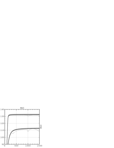
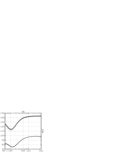
Figure 2.9: The renormalization scale dependence of $M_{h}$ introduced via the $\overline{\rm{DR}}$ definition of $\tan\beta$ and the Higgs field renormalization constants is shown as a function of $M_{A}$ (left plot) and $\tan\beta$ (right). The lower curves correspond to $\tan\beta=2$ (left) and $M_{A}=100\,\,\mathrm{GeV}$ (right). For the upper curves we have set $\tan\beta=20$ (left) and $M_{A}=500\,\,\mathrm{GeV}$ (right). $\mu_{\overline{\rm{DR}}}$ has been varied from $m_{t}/2$ to $2m_{t}$. The other parameters are chosen according to the $m_{h}^{\rm max}$ scenario, see the Appendix. The dotted line corresponds to the full on-shell scheme, see Sect. 2.3.4.

2.5.4 Estimate of the uncertainties from unknown three-loop corrections

Even in the case that a complete two-loop computation of the MSSM Higgs masses is achieved, non-negligible uncertainties will remain, due to the effect of higher-order corrections. Although a three-loop computation of the Higgs masses is not available so far, it is possible to give at least a rough estimate for the size of these unknown contributions.

A first estimate can be obtained by varying the renormalization scheme in which the parameters entering the two-loop part of the corrections are expressed. In fact, the resulting difference in the numerical results amounts formally to a three-loop effect. Since the ${\cal O}(\alpha_{t}\alpha_{s}+\alpha_{t}^{2})$ corrections are particularly sensitive to the value of the top mass, we compare the predictions for $M_{h}$ obtained using in the two-loop corrections either the top pole mass, $m_{t}^{\rm pole}=174.3\,\,\mathrm{GeV}$, or the SM running top mass $\overline{m}_{t}$, expressed in the $\overline{\rm{MS}}$ renormalization scheme, i.e.

$$\overline{m}_{t}\;\;\equiv\;\;m_{t}(m_{t})^{\overline{\rm{MS}}}_{\mathrm{SM}}\;\;\simeq\;\;\frac{m_{t}^{\rm pole}}{1+4\,\alpha_{s}(m_{t})/3\pi-\alpha_{t}(m_{t})/2\pi}~{}.$$ (2.133)

Figure 2.10: $M_{h}$ as a function of $X_{t}$, using either $m_{t}^{\rm pole}$ or $\overline{m}_{t}$ in the two-loop corrections. The relevant MSSM parameters are chosen as $\tan\beta=3\,,\,M_{\rm SUSY}=M_{A}=\mu=1\,\,\mathrm{TeV}$ and $m_{\tilde{g}}=800\,\,\mathrm{GeV}$. For the different lines see text.

Inserting appropriate values for the SM running couplings $\alpha_{s}$ and $\alpha_{t}$ we find $\overline{m}_{t}=168.6\,\,\mathrm{GeV}$. In Fig. 2.10 we show the effect of changing the renormalization scheme for $m_{t}$ in the two-loop part of the corrections. The relevant MSSM parameters are chosen as in Fig. 2.2, i.e. $\tan\beta=3\,,\;M_{\rm SUSY}=M_{A}=\mu=1\,\,\mathrm{TeV}$ and $m_{\tilde{g}}=800\,\,\mathrm{GeV}$. The dot–dashed and dotted curves show the ${\cal O}(\alpha_{t}\alpha_{s})$ predictions for $M_{h}$ obtained using $m_{t}^{\rm pole}$ or $\overline{m}_{t}$, respectively, in the two-loop corrections. The solid and dashed curves, instead, show the corresponding ${\cal O}(\alpha_{t}\alpha_{s}+\alpha_{t}^{2})$ predictions for $M_{h}$. The difference in the two latter curves induced by the shift in $m_{t}$, which should give an indication of the size of the unknown three-loop corrections, is of the order of 1–1.5 GeV. However, as can be seen from the figure, the effect of the shift in $m_{t}$ partially cancels between the ${\cal O}(\alpha_{t}\alpha_{s})$ and ${\cal O}(\alpha_{t}^{2})$ corrections, and there is no guarantee that such a compensating effect will appear again in the three-loop corrections.

An alternative way of estimating the typical size of the leading three-loop corrections makes use of the renormalization group approach. If all the supersymmetric particles (including the ${\cal CP}$-odd Higgs boson $A$) have the same mass $M_{\rm SUSY}$, and $\beta=\pi/2$, the effective theory at scales below $M_{\rm SUSY}$ is just the SM, with the role of the Higgs doublet played by the doublet that gives mass to the up-type quarks. In this simplified case, it is easy to apply the techniques of Refs. [14, 15] in order to obtain the leading logarithmic corrections to $M_{h}$ up to three loops (see also Ref. [68]). Considering, for further simplification, the case of zero stop mixing, we find

$$\left(\Delta M_{h}^{2}\right)^{\rm LL}=\frac{3\,\alpha_{t}\,\overline{m}_{t}^{2}}{\pi}\,t\,\left[\,1+\left(\frac{3}{8}\,\alpha_{t}-2\,\alpha_{s}\right)\,\frac{t}{\pi}+\left(\frac{23}{6}\,\alpha_{s}^{2}-\frac{5}{4}\,\alpha_{s}\alpha_{t}-\frac{33}{64}\,\alpha_{t}^{2}\right)\,\frac{t^{2}}{\pi^{2}}\,+...\,\right]\;,$$ (2.134)

where $t=\log\,(M_{\rm SUSY}^{2}/\overline{m}_{t}^{2})$, $\overline{m}_{t}$ is defined in eq. (2.133), $\alpha_{t}$ and $\alpha_{s}$ have to be interpreted as SM running quantities computed at the scale $Q=\overline{m}_{t}$, and the ellipses stand for higher loop contributions. It can be checked that, for $M_{\rm SUSY}=1\,\,\mathrm{TeV}$, the effect of the three-loop leading logarithmic terms amounts to an increase in $M_{h}$ of the order of 1–1.5 GeV. If $M_{\rm SUSY}$ is pushed to larger values, the relative importance of the higher-order logarithmic corrections obviously increases. In that case, it becomes necessary to resum the logarithmic corrections to all orders, by solving the appropriate renormalization group equations numerically. Since it is unlikely that a complete three-loop diagrammatic computation of the MSSM Higgs boson masses will be available in the near future, it will probably be necessary to combine different approaches (e.g. diagrammatic, effective potential, and renormalization group), in order to improve the accuracy of the theoretical predictions up to the level required to compare with the experimental results expected at the next generation of colliders.

To summarize this discussion, the uncertainty in the prediction for the lightest ${\cal CP}$-even Higgs boson arising from not yet calculated three-loop and even higher-order corrections can conservatively be estimated to be 1–2 GeV. From the various missing two-loop corrections an uncertainty of less than 1–2 GeV is expected. However, it is extremely unlikely that all these effects would coherently sum up, with no partial compensation among them. Therefore we believe that a realistic estimate of the uncertainty from unknown higher-order corrections in the theoretical prediction for the lightest Higgs boson mass should not exceed $3\,\,\mathrm{GeV}$.

2.6 Outlook

The current precision in the theory prediction of $M_{h}$, with an uncertainty of about $3\,\,\mathrm{GeV}$ from missing higher-order corrections and at least $4\,\,\mathrm{GeV}$ from parametric uncertainties can certainly not match the anticipated experimental precision at the LHC ($\Delta m_{h}\approx 200\,\,\mathrm{MeV}$) or at the LC ($\Delta m_{h}\approx 50\,\,\mathrm{MeV}$).

The intrinsic uncertainties from unknown higher-order corrections could be reduced to the level of $0.5\,\,\mathrm{GeV}$ or below, if a full two-loop calculation (including a proper renormalization) and leading/subleading three-loop (and possibly leading four-loop) calculations are available. On the other hand, the top quark mass will be measured extremely precisely at the LC [69], bringing down the parametric error induced by $m_{t}$ to the level of $0.1\,\,\mathrm{GeV}$. Also the other parametric uncertainties from SM parameters are expected to be reduced to this level.

If both the intrinsic and the parametric error will reduce as anticipated, the mass of the lightest Higgs boson $M_{h}$ can serve as an extremely accurate electroweak precision observable. It will be possible to use it to constrain unknown SUSY parameters, especially from the scalar top sector, see e.g. Refs. [70, 71, 72].

Chapter 3 The Higgs boson sector of the cMSSM

The radiative corrections to the Higgs boson masses in the ${\cal CP}$ conserving MSSM (rMSSM) are meanwhile quite advanced, as has been described in detail in Sect. 2. Comparisons of different methods, see e.g. Sect. 2.4, showing agreement where expected, have lead to deeper insight into the radiative corrections in the MSSM Higgs sector and thus to the confidence that the higher-order contribution, although being large, are under control.

In the case of the MSSM with complex parameters (cMSSM) the higher-order corrections have yet been restricted, after the first more general investigations [26], to evaluations in the EP approach [27] and to the RG improved one-loop EP method [28, 29]. These results have been restricted to the corrections coming from the (s)fermion sector and some leading logarithmic corrections from the gaugino sector. A more complete calculation has been attempted in Ref. [30]. More recently the leading one-loop corrections have also been evaluated in the FD method, using the on-shell renormalization scheme [31]. Some preliminary results including the full one-loop evaluation have been presented in Ref. [32]. The full one-loop result including a detailed phenomenological analysis can be found in Ref. [33, 47].

In this chapter we describe the full one-loop calculation in the FD approach using the on-shell renormalization scheme ($\overline{\rm{MS}}$ renormalization for $\tan\beta$ and the field renormalizations). Following Ref. [31], we present all analytical details of the calculation. The results are then briefly analyzed in view of the corrections coming from the non-(s)fermion sectors and the effects of the non-vanishing external momentum that can only be incorporated completely in the FD approach. For a more detailed analysis, see Ref. [33]. All results are incorporated into the public Fortran code FeynHiggs2.1  [73].

3.1 Tree-level relations and on-shell renormalization scheme

In this section we review the tree-level structure of of the MSSM, however with an emphasis on the ${\cal CP}$-violating parameters and their effects.

3.1.1 The scalar quark sector in the cMSSM

The mass matrix of two squarks of the same flavor, $\tilde{q}_{L}$ and $\tilde{q}_{R}$, is given by

$$M_{\tilde{q}}=\begin{pmatrix}M_{L}^{2}+m_{q}^{2}&m_{q}\;X_{q}^{*}\\ m_{q}\;X_{q}&M_{R}^{2}+m_{q}^{2}\end{pmatrix}$$ (3.1)

with

$$M_{L}^{2} = M_{\tilde{Q}}^{2}+M_{Z}^{2}\cos 2\beta\hskip 2.84526pt(I_{3}^{q}-Q_{q}s_{\mathrm{w}}^{2})$$

$$M_{R}^{2} = M_{\tilde{Q}^{\prime}}^{2}+M_{Z}^{2}\cos 2\beta\hskip 2.84526ptQ_{q}s_{\mathrm{w}}^{2}$$ (3.2)

$$X_{q} = A_{q}-\mu^{*}\{\cot\beta\hskip 2.84526pt,\tan\beta\},$$

where $\{\cot\beta\hskip 2.84526pt,\tan\beta\}$ applies for up- and down-type squarks, respectively. In the Higgs and scalar quark sector of the cMSSM $N_{q}+1$ phases are present, one for each $A_{q}$ and one for $\mu$, i.e. $N_{q}+1$ new parameters appear. As an abbreviation it will be used

$$\phi_{q}={\rm arg}\left(X_{q}\right).$$ (3.3)

As an independent parameter one can trade $\arg(A_{q})=\varphi_{A_{q}}$ for $\phi_{q}$.
The squark mass eigenstates are obtained by the rotation

$$\left(\begin{array}[]{c}\tilde{q}_{1}\\ \tilde{q}_{2}\end{array}\right)={\mathbf{U}}_{\tilde{q}}\left(\begin{array}[]{c}\tilde{q}_{L}\\ \tilde{q}_{R}\end{array}\right)$$ (3.4)

with

$${\mathbf{U}}_{\tilde{q}}=\left(\begin{array}[]{cc}c_{\tilde{q}}&s_{\tilde{q}}\\ -s_{\tilde{q}}^{*}&c_{\tilde{q}}\end{array}\right),\quad{\mathbf{U}}^{\tilde{q}+}{\mathbf{U}}^{\tilde{q}}={\rm 1\kern-1.19995pt\rule{0.3pt}{6.45831pt}\raisebox{0.0pt}{\rule{1.00006pt}{0.3pt}}}~{},$$ (3.5)

The mass eigenvalues are given by

$$m_{\tilde{q}_{1,2}}^{2}=m_{q}^{2}+\frac{1}{2}\left[M_{L}^{2}+M_{R}^{2}\mp\sqrt{(M_{L}^{2}-M_{R}^{2})^{2}+4m_{q}^{2}|X_{q}|^{2}}~{}\right],$$ (3.6)

and are independent of the phase of $X_{q}$. The elements of the mixing matrix ${\mathbf{U}}$ can be calculated as

$$c_{\tilde{q}}=\frac{\sqrt{M_{L}^{2}+m_{q}^{2}-m_{\tilde{q}_{2}}^{2}}}{\sqrt{m_{\tilde{q}_{1}}^{2}-m_{\tilde{q}_{2}}^{2}}},\quad s_{\tilde{q}}=\frac{X_{q}^{*}}{\sqrt{M_{L}^{2}+m_{q}^{2}-m_{\tilde{q}_{2}}^{2}}\sqrt{m_{\tilde{q}_{1}}^{2}-m_{\tilde{q}_{2}}^{2}}}.$$ (3.7)

The parameter $c_{\tilde{q}}\equiv\cos\theta\kern-1.49994pt_{\tilde{q}}$ is real, whereas $s_{\tilde{q}}\equiv e^{-i\phi_{q}}\,\sin\theta\kern-1.49994pt_{\tilde{q}}$ can be complex with the phase

$$\phi_{s_{\tilde{q}}}=-\phi_{q}={\rm arg}\left(X_{q}^{*}\right)~{}.$$ (3.8)

3.1.2 The chargino/neutralino sector in the cMSSM

The physical masses of the charginos can be determined from the matrix

$${\mathbf{X}}=\begin{pmatrix}M_{2}&\sqrt{2}\sin\beta\,M_{W}\\ \sqrt{2}\cos\beta\,M_{W}&\mu\end{pmatrix},$$ (3.9)

which contains the soft breaking term $M_{2}$ and the Higgs mass term $\mu$, both of which may take on complex values in the cMSSM. The rotation to the physical chargino mass eigenstates is done by transforming the original Wino and Higgsino fields with the help of two unitary 2$\times$2 matrices ${\mathbf{U}}$ and ${\mathbf{V}}$,

$$\begin{pmatrix}\tilde{\chi}_{1}^{+}\\ \tilde{\chi}_{2}^{+}\end{pmatrix}={\mathbf{V}}\begin{pmatrix}\tilde{W}^{+}\\ \tilde{H}_{1}^{+}\end{pmatrix},\quad\begin{pmatrix}\tilde{\chi}_{1}^{-}\\ \tilde{\chi}_{2}^{-}\end{pmatrix}={\mathbf{U}}\begin{pmatrix}\tilde{W}^{-}\\ \tilde{H}_{2}^{-}\end{pmatrix}$$ (3.10)

These definitions lead to the diagonal mass matrix

$$\begin{pmatrix}m_{\tilde{\chi}^{\pm}_{1}}&0\\ 0&m_{\tilde{\chi}^{\pm}_{2}}\end{pmatrix}={\mathbf{U}}^{*}\,{\mathbf{X}}\,{\mathbf{V}}^{+}.$$ (3.11)

From this relation, it becomes clear that the chargino masses $m_{\tilde{\chi}^{\pm}_{1}}$ and $m_{\tilde{\chi}^{\pm}_{2}}$ can be determined as the (real and positive) singular values of ${\mathbf{X}}$. The singular value decomposition of ${\mathbf{X}}$ also yields results for ${\mathbf{U}}$ and ${\mathbf{V}}$.

A similar procedure is used for the determination of the neutralino masses and mixing matrix, which can both be calculated from the mass matrix

$${\mathbf{Y}}=\begin{pmatrix}M_{1}&0&-M_{Z}\,s_{\mathrm{w}}\cos\beta\,&M_{Z}\,s_{\mathrm{w}}\sin\beta\,\\ 0&M_{2}&\quad M_{Z}\,c_{\mathrm{w}}\cos\beta\,&M_{Z}\,c_{\mathrm{w}}\sin\beta\,\\ -M_{Z}\,s_{\mathrm{w}}\cos\beta\,&M_{Z}\,c_{\mathrm{w}}\cos\beta\,&0&-\mu\\ \quad M_{Z}\,s_{\mathrm{w}}\sin\beta\,&M_{Z}\,c_{\mathrm{w}}\sin\beta\,&-\mu&0\end{pmatrix}.$$ (3.12)

This symmetric matrix contains the additional complex soft-breaking parameter $M_{1}$. Its diagonalization is achieved by a transformation starting from the original bino/wino/Higgsino basis,

$$\begin{pmatrix}\tilde{\chi}^{0}_{1}\\[5.0pt] \tilde{\chi}^{0}_{2}\\[5.0pt] \tilde{\chi}^{0}_{3}\\[5.0pt] \tilde{\chi}^{0}_{4}\end{pmatrix}={\mathbf{N}}\begin{pmatrix}\tilde{B}^{0}\\[5.0pt] \tilde{W}^{0}\\[5.0pt] \tilde{H}_{2}^{0}\\[5.0pt] \tilde{H}_{1}^{0}\end{pmatrix},\quad\begin{pmatrix}m_{\tilde{\chi}^{0}_{1}}&0&0&0\\[5.0pt] 0&m_{\tilde{\chi}^{0}_{2}}&0&0\\[5.0pt] 0&0&m_{\tilde{\chi}^{0}_{3}}&0\\[5.0pt] 0&0&0&m_{\tilde{\chi}^{0}_{4}}\end{pmatrix}={\mathbf{N}}^{*}\,{\mathbf{Y}}\,{\mathbf{N}}^{+}.$$ (3.13)

The unitary 4$\times$4 matrix ${\mathbf{N}}$ and the physical neutralino masses again result from a numerical singular value decomposition of ${\mathbf{Y}}$. The symmetry of ${\mathbf{Y}}$ permits the non-trivial condition of using only one matrix ${\mathbf{N}}$ for its diagonalization, in contrast to the chargino case shown above.

3.1.3 The cMSSM Higgs potential

The Higgs potential $V_{H}$ contains the real soft breaking terms $m_{1}^{2}$ and $m_{2}^{2}$, the potentially complex soft breaking parameter $m_{12}^{2}$ and the $U(1)$ and $SU(2)$ coupling constants $g_{1}$ and $g_{2}$:

$$V_{H} =m_{1}^{2}H_{1i}^{*}H_{1i}+m_{2}^{2}H_{2i}^{*}H_{2i}+\epsilon_{ij}(m_{12}^{2}H_{1i}H_{2j}+{m_{12}^{2}}^{*}H_{1i}^{*}H_{2j}^{*})$$

$$\quad+\tfrac{1}{8}(g_{1}^{2}+g_{2}^{2})(H_{1i}^{*}H_{1i}-H_{2i}^{*}H_{2i})^{2}+\tfrac{1}{2}g_{2}^{2}|H_{1i}^{*}H_{2i}|^{2}.$$ (3.14)

The indices $\{i,j\}=\{1,2\}$ refer to the respective Higgs doublet component, and $\epsilon_{12}=+1$. The Higgs doublets are decomposed in the following way,

$${\cal H}_{1}=\begin{pmatrix}H_{11}\\ H_{12}\end{pmatrix} =\begin{pmatrix}v_{1}+\tfrac{1}{\sqrt{2}}(\phi_{1}-i\chi_{1})\\ -\phi^{-}_{1}\end{pmatrix},$$

$${\cal H}_{2}=\begin{pmatrix}H_{21}\\ H_{22}\end{pmatrix} =e^{i\xi}\begin{pmatrix}\phi^{+}_{2}\\ v_{2}+\tfrac{1}{\sqrt{2}}(\phi_{2}+i\chi_{2})\end{pmatrix}.$$ (3.15)

As compared to the real case, see eq. (2.11), besides the vacuum expectation values $v_{1}$ and $v_{2}$, eq. (3.1.3) introduces a real, as yet undetermined, possible new phase $\xi$ between the two Higgs doublets. Using this decomposition, $V_{H}$ can be rearranged in powers of the fields,

$$V_{H} =\cdots-T_{\phi_{1}}\phi_{1}-T_{\phi_{2}}\phi_{2}-T_{\chi_{1}}\chi_{1}-T_{\chi_{2}}\chi_{2}$$

$$+\tfrac{1}{2}\begin{pmatrix}\phi_{1},\phi_{2},\chi_{1},\chi_{2}\end{pmatrix}{\mathbf{M}}_{\mathrm{n}}\begin{pmatrix}\phi_{1}\\ \phi_{2}\\ \chi_{1}\\ \chi_{2}\end{pmatrix}+\begin{pmatrix}\phi^{-}_{1},\phi^{-}_{2}\end{pmatrix}{\mathbf{M}}_{\mathrm{c}}\begin{pmatrix}\phi^{+}_{1}\\ \phi^{+}_{2}\end{pmatrix}+\cdots,$$ (3.16)

where the coefficients of the linear terms are the tadpoles and those of the quadratic terms are the mass matrices ${\mathbf{M}}_{\mathrm{n}}$ and ${\mathbf{M}}_{\mathrm{c}}$. The tadpole coefficients read

$$T_{\phi_{1}} =-\sqrt{2}(m_{1}^{2}v_{1}+\cos\xi^{\prime}|m_{12}^{2}|v_{2}+\tfrac{1}{4}(g_{1}^{2}+g_{2}^{2})(v_{1}^{2}-v_{2}^{2})v_{1}),$$ (3.17a)

$$T_{\phi_{2}} =-\sqrt{2}(m_{2}^{2}v_{2}+\cos\xi^{\prime}|m_{12}^{2}|v_{1}-\tfrac{1}{4}(g_{1}^{2}+g_{2}^{2})(v_{1}^{2}-v_{2}^{2})v_{2}),$$ (3.17b)

$$T_{\chi_{1}} =-\sqrt{2}\sin\xi^{\prime}|m_{12}^{2}|v_{1}=-T_{\chi_{2}},$$ (3.17c)

with $\xi^{\prime}:=\xi+\arg(m_{12}^{2})$.

The real, symmetric 4$\times$4-matrix ${\mathbf{M}}_{\mathrm{n}}$ and the hermitian 2$\times$2-matrix ${\mathbf{M}}_{\mathrm{c}}$ contain the following elements,

$${\mathbf{M}}_{\mathrm{n}} =\begin{pmatrix}{\mathbf{M}}_{\phi}&{\mathbf{M}}_{\phi\chi}\\[5.0pt] {\mathbf{M}}_{\phi\chi}&{\mathbf{M}}_{\chi}\end{pmatrix},$$ (3.18a)

$${\mathbf{M}}_{\phi} =\begin{pmatrix}m_{1}^{2}+\tfrac{1}{4}(g_{1}^{2}+g_{2}^{2})(3v_{1}^{2}-v_{2}^{2})&\cos\xi^{\prime}|m_{12}^{2}|-\tfrac{1}{2}(g_{1}^{2}+g_{2}^{2})v_{1}v_{2}\\[5.0pt] \cos\xi^{\prime}|m_{12}^{2}|-\tfrac{1}{2}(g_{1}^{2}+g_{2}^{2})v_{1}v_{2}&m_{2}^{2}+\tfrac{1}{4}(g_{1}^{2}+g_{2}^{2})(3v_{2}^{2}-v_{1}^{2})\end{pmatrix},$$ (3.18b)

$${\mathbf{M}}_{\phi\chi} =\begin{pmatrix}0&-\sin\xi^{\prime}|m_{12}^{2}|\\[5.0pt] \sin\xi^{\prime}|m_{12}^{2}|&0\end{pmatrix},$$ (3.18c)

$${\mathbf{M}}_{\chi} =\begin{pmatrix}m_{1}^{2}+\tfrac{1}{4}(g_{1}^{2}+g_{2}^{2})(v_{1}^{2}-v_{2}^{2})&\cos\xi^{\prime}|m_{12}^{2}|\\[5.0pt] \cos\xi^{\prime}|m_{12}^{2}|&m_{2}^{2}+\tfrac{1}{4}(g_{1}^{2}+g_{2}^{2})(v_{2}^{2}-v_{1}^{2})\end{pmatrix},$$ (3.18d)

$${\mathbf{M}}_{\mathrm{c}} =\begin{pmatrix}m_{1}^{2}+\tfrac{1}{4}g_{1}^{2}(v_{1}^{2}-v_{2}^{2})+\tfrac{1}{4}g_{2}^{2}(v_{1}^{2}+v_{2}^{2})&e^{i\xi^{\prime}}|m_{12}^{2}|-\tfrac{1}{2}g_{2}^{2}v_{1}v_{2}\\[5.0pt] e^{-i\xi^{\prime}}|m_{12}^{2}|-\tfrac{1}{2}g_{2}^{2}v_{1}v_{2}&m_{2}^{2}+\tfrac{1}{4}g_{1}^{2}(v_{2}^{2}-v_{1}^{2})+\tfrac{1}{4}g_{2}^{2}(v_{1}^{2}+v_{2}^{2})\end{pmatrix}.$$ (3.18e)

The non-vanishing elements of ${\mathbf{M}}_{\phi\chi}$ lead to ${\cal CP}$-violating mixing terms in the Higgs potential between the ${\cal CP}$-even fields $\phi_{1}$ and $\phi_{2}$ and the ${\cal CP}$-odd fields $\chi_{1}$ and $\chi_{2}$ if $\xi^{\prime}\neq 0$. The physically relevant mass eigenstates in lowest order follow from a unitary transformation of the original fields,

$$\begin{pmatrix}h\\ H\\ A\\ G\end{pmatrix}={\mathbf{U}}_{\mathrm{n}(0)}\cdot\begin{pmatrix}\phi_{1}\\ \phi_{2}\\ \chi_{1}\\ \chi_{2}\end{pmatrix},\quad\begin{pmatrix}H^{\pm}\\ G^{\pm}\end{pmatrix}={\mathbf{U}}_{\mathrm{c}(0)}\cdot\begin{pmatrix}\phi_{1}^{\pm}\\ \phi_{2}^{\pm}\end{pmatrix},$$ (3.19)

such that the resulting mass matrices

$${\mathbf{M}}_{\mathrm{n}}^{\rm diag}={\mathbf{U}}_{\mathrm{n}(0)}{\mathbf{M}}_{\mathrm{n}}{\mathbf{U}}_{\mathrm{n}(0)}^{+}\quad{\rm and}\quad{\mathbf{M}}_{\mathrm{c}}^{\rm diag}={\mathbf{U}}_{\mathrm{c}(0)}{\mathbf{M}}_{\mathrm{c}}{\mathbf{U}}_{\mathrm{c}(0)}^{+}$$ (3.20)

of the new fields will be diagonal. The new fields correspond to the three neutral Higgs bosons $h$, $H$ and $A$, the charged pair $H^{\pm}$ and the Goldstone bosons $G$ and $G^{\pm}$.

The lowest-order mixing matrices can be determined from the eigenvectors of ${\mathbf{M}}_{\mathrm{n}}$ and ${\mathbf{M}}_{\mathrm{c}}$, calculated under the additional condition that the tadpole coefficients (3.17) must vanish in order that $v_{1}$ and $v_{2}$ are indeed stationary points of the Higgs potential. This automatically requires $\xi^{\prime}=0$, which in turn leads to a vanishing matrix ${\mathbf{M}}_{\phi\chi}$ and a real, symmetric matrix ${\mathbf{M}}_{\mathrm{c}}$. Therefore, no ${\cal CP}$-violation occurs in the Higgs potential at the lowest order, and the corresponding mixing matrices can be parametrized by real mixing angles as

$${\mathbf{U}}_{\mathrm{n}(0)}=\begin{pmatrix}-\sin\alpha\,&\cos\alpha\,&0&0\\ \quad\cos\alpha\,&\sin\alpha\,&0&0\\ 0&0&-\sin\beta_{\mathrm{n}}&\cos\beta_{\mathrm{n}}\\ 0&0&\quad\cos\beta_{\mathrm{n}}&\sin\beta_{\mathrm{n}}\end{pmatrix},\quad{\mathbf{U}}_{\mathrm{c}(0)}=\begin{pmatrix}-\sin\beta_{\mathrm{c}}&\cos\beta_{\mathrm{c}}\\ \quad\cos\beta_{\mathrm{c}}&\sin\beta_{\mathrm{c}}\end{pmatrix}.$$ (3.21)

The mixing angles $\alpha$, $\beta_{\mathrm{n}}$ and $\beta_{\mathrm{c}}$ can be determined from the requirement that this transformation will result in diagonal mass matrices for the physical fields.

3.1.4 Higgs mass terms and tadpoles

The terms in $V_{H}$ that are linear or quadratic in the physical fields are denoted as follows,

$$V_{H} =\mathrm{const.}-T_{h}\cdot h-T_{H}\cdot H-T_{A}\cdot A-T_{G}\cdot G$$

$$\quad+\tfrac{1}{2}\begin{pmatrix}h,H,A,G\end{pmatrix}\cdot\begin{pmatrix}m_{h}^{2}&m_{hH}^{2}&m_{hA}^{2}&m_{hG}^{2}\\ m_{hH}^{2}&m_{H}^{2}&m_{HA}^{2}&m_{HG}^{2}\\ m_{hA}^{2}&m_{HA}^{2}&m_{A}^{2}&m_{AG}^{2}\\ m_{hG}^{2}&m_{HG}^{2}&m_{AG}^{2}&m_{G}^{2}\end{pmatrix}\cdot\begin{pmatrix}h\\ H\\ A\\ G\end{pmatrix}+$$ (3.22)

$$\quad+\begin{pmatrix}H^{-},G^{-}\end{pmatrix}\cdot\begin{pmatrix}m_{H^{\pm}}^{2}&m_{H^{-}G^{+}}^{2}\\ m_{G^{-}H^{+}}^{2}&m_{G^{\pm}}^{2}\end{pmatrix}\cdot\begin{pmatrix}H^{+}\\ G^{+}\end{pmatrix}+\cdots.$$

In order to perform a simple renormalization procedure, the parameters in $V_{H}$ have to be expressed in term of physical parameters. In total, $V_{H}$ contains eight independent real parameters: $v_{1}$, $v_{2}$, $g_{1}^{2}$, $g_{2}^{2}$, $m_{1}^{2}$, $m_{2}^{2}$, $|m_{12}^{2}|$ and $\arg(m_{12}^{2})$ (or $\xi^{\prime}$). The coupling constants $g_{1}$ and $g_{2}$ can be replaced by the electric coupling constant $e$ and the weak mixing angle $\theta_{\mathrm{w}}$ ($s_{\mathrm{w}}\equiv\sin\theta_{\mathrm{w}}$, $c_{\mathrm{w}}\equiv\cos\theta_{\mathrm{w}}$),

$$e=g_{1}\,c_{\mathrm{w}}=g_{2}\,s_{\mathrm{w}},$$ (3.23)

while the $Z$ boson mass $M_{Z}$ and $\tan\beta$ substitute for $v_{1}$ and $v_{2}$:

$$\tan\beta=\frac{v_{2}}{v_{1}},\;M_{Z}^{2}=\tfrac{1}{2}(g_{1}^{2}+g_{2}^{2})(v_{1}^{2}+v_{2}^{2}).$$ (3.24)

The $W$ boson mass is then given by

$$M_{W}=\frac{1}{2}g_{2}^{2}(v_{1}^{2}+v_{2}^{2}).$$ (3.25)

The tadpole coefficients in the physical basis follow from the original ones (3.17) by applying the transformation (3.21),

$$T_{H} =\sqrt{2}[-m_{1}^{2}v_{1}\cos\alpha\,-m_{2}^{2}v_{2}\sin\alpha\,-\cos\xi^{\prime}|m_{12}^{2}|(v_{1}\sin\alpha\,+v_{2}\cos\alpha\,)$$ (3.26a)

$$\quad-\tfrac{1}{4}(g_{1}^{2}+g_{2}^{2})(v_{1}^{2}-v_{2}^{2})(v_{1}\cos\alpha\,-v_{2}\sin\alpha\,)],$$

$$T_{h} =\sqrt{2}[+m_{1}^{2}v_{1}\sin\alpha\,-m_{2}^{2}v_{2}\cos\alpha\,-\cos\xi^{\prime}|m_{12}^{2}|(v_{1}\cos\alpha\,-v_{2}\sin\alpha\,)$$ (3.26b)

$$\quad+\tfrac{1}{4}(g_{1}^{2}+g_{2}^{2})(v_{1}^{2}-v_{2}^{2})(v_{1}\sin\alpha\,+v_{2}\cos\alpha\,)],$$

$$T_{A} =\sqrt{2}\sin\xi^{\prime}|m_{12}^{2}|(v_{1}\cos\beta_{\mathrm{n}}+v_{2}\sin\beta_{\mathrm{n}}),$$ (3.26c)

$$T_{G} =-\tan(\beta-\beta_{\mathrm{n}})T_{A}.$$ (3.26d)

Due to the linear dependence of $T_{G}$ on $T_{A}$, eq. (3.26) provides only three replacements for the original parameters. Typically, the remaining parameter is replaced by either the mass of the neutral $A$-boson, $m_{A}$, or the mass of the charged pair, $m_{H^{\pm}}$. Their expressions in terms of the original parameters are given by

$$m_{A}^{2} =m_{1}^{2}\sin^{2}\beta_{\mathrm{n}}+m_{2}^{2}\cos^{2}\beta_{\mathrm{n}}-\sin 2\beta_{\mathrm{n}}\cos\xi^{\prime}|m_{12}^{2}|$$

$$\quad-\cos 2\beta_{\mathrm{n}}\tfrac{1}{4}(g_{1}^{2}+g_{2}^{2})(v_{1}^{2}-v_{2}^{2}),$$ (3.27a)

$$m_{H^{\pm}}^{2} =m_{1}^{2}\sin^{2}\beta_{\mathrm{c}}+m_{2}^{2}\cos^{2}\beta_{\mathrm{c}}-\sin 2\beta_{\mathrm{c}}\cos\xi^{\prime}|m_{12}^{2}|$$

$$\quad-\cos 2\beta_{\mathrm{c}}\tfrac{1}{4}(g_{1}^{2}+g_{2}^{2})(v_{1}^{2}-v_{2}^{2})+\tfrac{1}{2}g_{2}^{2}(v_{1}\cos\beta_{\mathrm{c}}+v_{2}\sin\beta_{\mathrm{c}})^{2}.$$ (3.27b)

If $\beta_{\mathrm{n}}=\beta_{\mathrm{c}}$ (what will be shown below) the relation between $m_{A}^{2}$ and $m_{H^{\pm}}^{2}$ becomes

$$m_{H^{\pm}}^{2}=m_{A}^{2}+M_{W}^{2}~{}.$$ (3.28)

Using (3.26a-c) and (3.27) or (3.27), all of $m_{1}^{2}$, $m_{2}^{2}$, $|m_{12}^{2}|$ and $\xi^{\prime}$ can be substituted by $T_{h}$, $T_{H}$, $T_{A}$ and ($m_{A}$ or $m_{H^{\pm}}$). In summary, this leads to the following replacements:

$$v_{1} \to\frac{\sqrt{2}\,\cos\beta\hskip 2.84526pt\,s_{\mathrm{w}}\,c_{\mathrm{w}}\,M_{Z}}{e},$$ (3.29)

$$v_{2} \to\frac{\sqrt{2}\,\sin\beta\,s_{\mathrm{w}}\,c_{\mathrm{w}}\,M_{Z}}{e},$$ (3.30)

$$g_{1} \to e/c_{\mathrm{w}},$$ (3.31)

$$g_{2} \to e/s_{\mathrm{w}},$$ (3.32)

$$m_{1}^{2} \to-\frac{1}{8}\Big{[}-4m_{A}^{2}+2(2m_{A}^{2}+M_{Z}^{2})\cos 2\beta\hskip 2.84526pt+M_{Z}^{2}\cos(4\beta-2\beta_{\mathrm{n}})+M_{Z}^{2}\cos(2\beta_{\mathrm{n}})$$ (3.33)

$$+\frac{eT_{h}\cos\beta_{\mathrm{n}}}{2c_{\mathrm{w}}s_{\mathrm{w}}M_{Z}}\left(\cos\beta\hskip 2.84526pt\cos\beta_{\mathrm{n}}\sin\alpha\hskip 2.84526pt+\sin\beta(\cos\alpha\hskip 2.84526pt\cos\beta_{\mathrm{n}}+2\sin\alpha\hskip 2.84526pt\sin\beta_{\mathrm{n}})\right)$$

$$+\frac{eT_{H}\cos\beta_{\mathrm{n}}}{2c_{\mathrm{w}}s_{\mathrm{w}}M_{Z}}\left(\cos\beta_{\mathrm{n}}\sin\alpha\hskip 2.84526pt\sin\beta-\cos\alpha\hskip 2.84526pt(\cos\beta\hskip 2.84526pt\cos\beta_{\mathrm{n}}+2\sin\beta\sin\beta_{\mathrm{n}})\right)\Big{]}/\left(\cos^{2}(\beta-\beta_{\mathrm{n}})\right),$$

$$m_{2}^{2} \to\frac{1}{8}\Big{[}4m_{A}^{2}+2(2m_{A}^{2}+M_{Z}^{2})\cos 2\beta\hskip 2.84526pt+M_{Z}^{2}\cos(4\beta-2\beta_{\mathrm{n}})+M_{Z}^{2}\cos(2\beta_{\mathrm{n}})$$ (3.34)

$$-\frac{eT_{h}\sin\beta_{\mathrm{n}}}{2c_{\mathrm{w}}s_{\mathrm{w}}M_{Z}}\left(\cos\beta\hskip 2.84526pt\sin\beta_{\mathrm{n}}\sin\alpha\hskip 2.84526pt+\cos\alpha\hskip 2.84526pt(\sin\beta\sin\beta_{\mathrm{n}}+2\cos\beta\hskip 2.84526pt\cos\beta_{\mathrm{n}})\right)$$

$$-\frac{eT_{H}\sin\beta_{\mathrm{n}}}{4c_{\mathrm{w}}s_{\mathrm{w}}M_{Z}}\left(2\sin\alpha\hskip 2.84526pt\sin\beta\sin\beta_{\mathrm{n}}+\cos\beta\hskip 2.84526pt(3\sin(\alpha-\beta_{\mathrm{n}})+\sin(\alpha+\beta_{\mathrm{n}})\right)\Big{]}/\left(\cos^{2}(\beta-\beta_{\mathrm{n}})\right),$$

$$|m_{12}^{2}| \to\sqrt{\left(f_{m}^{2}+f_{s}^{2}\right)}$$ (3.35)

$${}f_{m}=\Big{[}\frac{1}{2}m_{A}^{2}\sin 2\beta\hskip 2.84526pt-\frac{eT_{h}}{4c_{\mathrm{w}}s_{\mathrm{w}}M_{Z}}\left(\cos(\beta+\alpha)+\cos(\beta-\alpha)\hskip 2.84526pt\cos(2\beta_{\mathrm{n}})\right)$$

$${}~{}~{}~{}~{}~{}~{}~{}-\frac{eT_{H}}{4c_{\mathrm{w}}s_{\mathrm{w}}M_{Z}}\left(\sin(\beta+\alpha)+\sin(\beta-\alpha)\hskip 2.84526pt\cos(2\beta_{\mathrm{n}})\right)\Big{]}/\left(\cos^{2}(\beta-\beta_{\mathrm{n}})\right),$$

$${}f_{s}=\frac{eT_{A}}{2s_{\mathrm{w}}c_{\mathrm{w}}M_{Z}\left(\cos\beta\hskip 2.84526pt\cos\beta_{\mathrm{n}}+\sin\beta\sin\beta_{\mathrm{n}}\right)},$$

$$\sin\xi^{\prime} \to f_{s}/\sqrt{f_{m}^{2}+f_{s}^{2}},$$ (3.36)

$$\cos\xi^{\prime} \to f_{m}/\sqrt{f_{m}^{2}+f_{s}^{2}}~{}.$$ (3.37)

The resulting physical mass terms are given either in terms of $m_{A}$ or $m_{H^{\pm}}$, depending on which parameter leads to more compact expressions.

The charged Higgs sector contains, apart from $m_{H^{\pm}}^{2}$, the mass terms

$$m_{H^{-}G^{+}}^{2} =-m_{H^{\pm}}^{2}\tan(\beta-\beta_{\mathrm{c}})$$ (3.38a)

$$\quad-\tfrac{e}{2M_{Z}s_{\mathrm{w}}c_{\mathrm{w}}}T_{H}\sin(\alpha-\beta_{\mathrm{c}})/\cos(\beta-\beta_{\mathrm{c}})$$

$$\quad-\tfrac{e}{2M_{Z}s_{\mathrm{w}}c_{\mathrm{w}}}T_{h}\cos(\alpha-\beta_{\mathrm{c}})/\cos(\beta-\beta_{\mathrm{c}})$$

$$\quad-\tfrac{e}{2M_{Z}s_{\mathrm{w}}c_{\mathrm{w}}}iT_{A}/\cos(\beta-\beta_{\mathrm{n}}),$$

$$m_{G^{-}H^{+}}^{2} =(m_{H^{-}G^{+}}^{2})^{*},$$ (3.38b)

$$m_{G^{\pm}}^{2} =m_{H^{\pm}}^{2}\tan^{2}(\beta-\beta_{\mathrm{c}})$$

$$\quad-\tfrac{e}{2M_{Z}s_{\mathrm{w}}c_{\mathrm{w}}}T_{H}\cos(\alpha+\beta-2\beta_{\mathrm{c}})/\cos^{2}(\beta-\beta_{\mathrm{c}})$$ (3.38c)

$$\quad+\tfrac{e}{2M_{Z}s_{\mathrm{w}}c_{\mathrm{w}}}T_{h}\sin(\alpha+\beta-2\beta_{\mathrm{c}})/\cos^{2}(\beta-\beta_{\mathrm{c}}),$$ (3.38d)

where the star denotes a complex conjugation.

The neutral mass matrix is more easily parametrized by $m_{A}$, as can be seen from the 2$\times$2 sub-matrix of the $A$ and $G$ boson:

$$m_{AG}^{2} =-m_{A}^{2}\tan(\beta-\beta_{\mathrm{n}})$$ (3.39a)

$$\quad-\tfrac{e}{2M_{Z}s_{\mathrm{w}}c_{\mathrm{w}}}T_{H}\sin(\alpha-\beta_{\mathrm{n}})/\cos(\beta-\beta_{\mathrm{n}})$$

$$\quad-\tfrac{e}{2M_{Z}s_{\mathrm{w}}c_{\mathrm{w}}}T_{h}\cos(\alpha-\beta_{\mathrm{n}})/\cos(\beta-\beta_{\mathrm{n}}),$$

$$m_{G}^{2} =m_{A}^{2}\tan^{2}(\beta-\beta_{\mathrm{n}})$$ (3.39b)

$$\quad-\tfrac{e}{2M_{Z}s_{\mathrm{w}}c_{\mathrm{w}}}T_{H}\cos(\alpha+\beta-2\beta_{\mathrm{n}})/\cos^{2}(\beta-\beta_{\mathrm{n}})$$

$$\quad+\tfrac{e}{2M_{Z}s_{\mathrm{w}}c_{\mathrm{w}}}T_{h}\sin(\alpha+\beta-2\beta_{\mathrm{n}})/\cos^{2}(\beta-\beta_{\mathrm{n}}).$$ (3.39c)

The ${\cal CP}$-violating mixing terms connecting the $h$-/$H$- and the $A$-/$G$-sector are

$$m_{hA}^{2} =\tfrac{e}{2M_{Z}s_{\mathrm{w}}c_{\mathrm{w}}}T_{A}\sin(\alpha-\beta_{\mathrm{n}})/\cos(\beta-\beta_{\mathrm{n}}),$$ (3.40a)

$$m_{hG}^{2} =\tfrac{e}{2M_{Z}s_{\mathrm{w}}c_{\mathrm{w}}}T_{A}\cos(\alpha-\beta_{\mathrm{n}})/\cos(\beta-\beta_{\mathrm{n}}),$$ (3.40b)

$$m_{HA}^{2} =-m_{hG}^{2},$$ (3.40c)

$$m_{HG}^{2} =\tfrac{e}{2M_{Z}s_{\mathrm{w}}c_{\mathrm{w}}}T_{A}\sin(\alpha-\beta_{\mathrm{n}})/\cos(\beta-\beta_{\mathrm{n}}).$$ (3.40d)

Finally, the mass terms of the ${\cal CP}$-even $h$ and $H$ bosons are:

$$m_{h}^{2} =M_{Z}^{2}\sin^{2}(\alpha+\beta)$$ (3.41a)

$$\quad+m_{A}^{2}\cos^{2}(\alpha-\beta)/\cos^{2}(\beta-\beta_{\mathrm{n}})$$

$$\quad+\tfrac{e}{2M_{Z}s_{\mathrm{w}}c_{\mathrm{w}}}T_{H}\cos(\alpha-\beta)\sin^{2}(\alpha-\beta_{\mathrm{n}})/\cos^{2}(\beta-\beta_{\mathrm{n}})$$

$$\quad+\tfrac{e}{2M_{Z}s_{\mathrm{w}}c_{\mathrm{w}}}T_{h}\tfrac{1}{2}\sin(\alpha-\beta_{\mathrm{n}})(\cos(2\alpha-\beta-\beta_{\mathrm{n}})+3\cos(\beta-\beta_{\mathrm{n}}))/\cos^{2}(\beta-\beta_{\mathrm{n}}),$$

$$m_{hH}^{2} =-M_{Z}^{2}\sin(\alpha+\beta)\cos(\alpha+\beta)$$ (3.41b)

$$\quad+m_{A}^{2}\sin(\alpha-\beta)\cos(\alpha-\beta)/\cos^{2}(\beta-\beta_{\mathrm{n}})$$

$$\quad+\tfrac{e}{2M_{Z}s_{\mathrm{w}}c_{\mathrm{w}}}T_{H}\sin(\alpha-\beta)\sin^{2}(\alpha-\beta_{\mathrm{n}})/\cos^{2}(\beta-\beta_{\mathrm{n}})$$

$$\quad-\tfrac{e}{2M_{Z}s_{\mathrm{w}}c_{\mathrm{w}}}T_{h}\cos(\alpha-\beta)\cos^{2}(\alpha-\beta_{\mathrm{n}})/\cos^{2}(\beta-\beta_{\mathrm{n}}),$$

$$m_{H}^{2} =M_{Z}^{2}\cos^{2}(\alpha+\beta)$$ (3.41c)

$$\quad+m_{A}^{2}\sin^{2}(\alpha-\beta)/\cos^{2}(\beta-\beta_{\mathrm{n}})$$

$$\quad+\tfrac{e}{2M_{Z}s_{\mathrm{w}}c_{\mathrm{w}}}T_{H}\tfrac{1}{2}\cos(\alpha-\beta_{\mathrm{n}})(\cos(2\alpha-\beta-\beta_{\mathrm{n}})-3\cos(\beta-\beta_{\mathrm{n}}))/\cos^{2}(\beta-\beta_{\mathrm{n}})$$

$$\quad-\tfrac{e}{2M_{Z}s_{\mathrm{w}}c_{\mathrm{w}}}T_{h}\sin(\alpha-\beta)\cos^{2}(\alpha-\beta_{\mathrm{n}})/\cos^{2}(\beta-\beta_{\mathrm{n}}).$$

3.1.5 Masses and mixing angles in lowest order

The masses and mixing angles in lowest order follow from eqs. (3.38)-(3.41) and the additional requirement that both the tadpole coefficients $T_{\{h,H,A\}}$ and all non-diagonal entries of the mass matrices must vanish. From (3.38a) and (3.39a), it immediately follows that

$$\beta_{\mathrm{c}}=\beta_{\mathrm{n}}=\beta,$$ (3.42)

which in turn determines the tree-level value of $\alpha=\alpha_{(0)}$ (up to a sign) from (3.41b) as (which is equivalent to eq. (2.33) in the rMSSM)

$$\tan 2\alpha_{(0)}=\tan 2\beta\frac{m_{A}^{2}+M_{Z}^{2}}{m_{A}^{2}-M_{Z}^{2}},\quad-\frac{\pi}{2}\leq\alpha_{(0)}\leq 0~{}.$$ (3.43)

The Higgs masses $m_{h(0)}$ and $m_{H(0)}$ are the eigenvalues of their 2$\times$2 mass matrix with entries (3.41, $\alpha$ set to zero),

$$\{m_{h(0)}^{2},m_{H(0)}^{2}\}=\tfrac{1}{2}\left(m_{A}^{2}+M_{Z}^{2}\mp\sqrt{(m_{A}^{2}+M_{Z}^{2})^{2}-4m_{A}^{2}M_{Z}^{2}\cos^{2}2\beta}\right).$$ (3.44a)

Finally, combining eqs. (3.27) and (3.42) relates the remaining masses $m_{A}$ and $m_{H^{\pm}}$ with each other,

$$m_{H^{\pm}}^{2}=m_{A}^{2}+c_{\mathrm{w}}^{2}M_{Z}^{2}=m_{A}^{2}+M_{W}^{2}.$$ (3.45)

Specifying one Higgs boson mass as an input parameter therefore unambiguously determines the other ones. Since the ${\cal CP}$-odd $A$ boson will –due to the ${\cal CP}$-violating mixing in the neutral Higgs sector– no longer be an eigenstate in higher orders, the charged Higgs mass $m_{H^{\pm}}$ will be used as input parameter in the cMSSM.

3.1.6 Renormalization of the Higgs potential

In this and the following sections we will focus one the one-loop corrections to the cMSSM Higgs sector. However, two-loop corrections (taken from the rMSSM, see Refs. [16, 5, 7]) will be included in our numerical evaluation, see Sect. 3.3.

In order to calculate the first-order corrections to the Higgs boson masses and effective mixing angles, the counter terms for the mass and tadpole coefficients in the Higgs potential are needed. Apart from these, counter terms are needed for several other parameters which appear in the Higgs potential:

$$M_{Z}^{2} \rightarrow M_{Z}^{2}+\delta M_{Z}^{2}, T_{h} \rightarrow T_{h}+\delta T_{h},$$ (3.46)

$$M_{W}^{2} \rightarrow M_{W}^{2}+\delta M_{W}^{2}, T_{H} \rightarrow T_{H}+\delta T_{H},$$

$${\mathbf{M}}_{\mathrm{n}} \rightarrow{\mathbf{M}}_{\mathrm{n}}+\delta{\mathbf{M}}_{\mathrm{n}}, T_{A} \rightarrow T_{A}+\delta T_{A},$$

$${\mathbf{M}}_{\mathrm{c}} \rightarrow{\mathbf{M}}_{\mathrm{c}}+\delta{\mathbf{M}}_{\mathrm{c}}, \tan\beta\, \rightarrow\tan\beta\,(1+\delta\!\tan\!\beta\,).$$

These definitions explain why the expressions (3.38-3.41) for the Higgs masses must differentiate between the mixing angles $\beta_{\mathrm{n}}$ and $\beta_{\mathrm{c}}$ (which, like $\alpha$, are not renormalized) and the parameter $\beta$ (which is). This distinction is necessary to arrive at the following expressions for the counter terms.

The field renormalization matrices of both Higgs multiplets can be set up symmetrically,

$$\begin{pmatrix}h\\[5.0pt] H\\[5.0pt] A\\[5.0pt] G\end{pmatrix}\rightarrow\begin{pmatrix}1+\tfrac{1}{2}\delta Z_{hh}&\tfrac{1}{2}\delta Z_{hH}&\tfrac{1}{2}\delta Z_{hA}&\tfrac{1}{2}\delta Z_{hG}\\[5.0pt] \tfrac{1}{2}\delta Z_{hH}&1+\tfrac{1}{2}\delta Z_{HH}&\tfrac{1}{2}\delta Z_{HA}&\tfrac{1}{2}\delta Z_{HG}\\[5.0pt] \tfrac{1}{2}\delta Z_{hA}&\tfrac{1}{2}\delta Z_{HA}&1+\tfrac{1}{2}\delta Z_{AA}&\tfrac{1}{2}\delta Z_{AG}\\[5.0pt] \tfrac{1}{2}\delta Z_{hG}&\tfrac{1}{2}\delta Z_{HG}&\tfrac{1}{2}\delta Z_{AG}&1+\tfrac{1}{2}\delta Z_{GG}\end{pmatrix}\cdot\begin{pmatrix}h\\[5.0pt] H\\[5.0pt] A\\[5.0pt] G\end{pmatrix}$$ (3.47a)

and

$$\begin{pmatrix}H^{+}\\[5.0pt] G^{+}\end{pmatrix} \rightarrow\begin{pmatrix}1+\tfrac{1}{2}\delta Z_{H^{+}}&\tfrac{1}{2}\delta Z_{H^{-}G^{+}}\\[5.0pt] \tfrac{1}{2}\delta Z_{G^{-}H^{+}}&1+\tfrac{1}{2}\delta Z_{G^{+}}\end{pmatrix}\cdot\begin{pmatrix}H^{+}\\[5.0pt] G^{+}\end{pmatrix},$$ (3.47b)

$$\begin{pmatrix}H^{-}\\[5.0pt] G^{-}\end{pmatrix} \rightarrow\begin{pmatrix}1+\tfrac{1}{2}\delta Z_{H^{+}}^{*}&\tfrac{1}{2}\delta Z_{G^{-}H^{+}}\\[5.0pt] \tfrac{1}{2}\delta Z_{H^{-}G^{+}}&1+\tfrac{1}{2}\delta Z_{G^{+}}^{*}\end{pmatrix}\cdot\begin{pmatrix}H^{-}\\[5.0pt] G^{-}\end{pmatrix}.$$ (3.47c)

For the mass counter term matrices we use the definitions

$$\delta{\mathbf{M}}_{\mathrm{n}}=\begin{pmatrix}\delta m_{h}^{2}&\delta m_{hH}^{2}&\delta m_{hA}^{2}&\delta m_{hG}^{2}\\[5.0pt] \delta m_{hH}^{2}&\delta m_{H}^{2}&\delta m_{HA}^{2}&\delta m_{HG}^{2}\\[5.0pt] \delta m_{hA}^{2}&\delta m_{HA}^{2}&\delta m_{A}^{2}&\delta m_{AG}^{2}\\[5.0pt] \delta m_{hG}^{2}&\delta m_{HG}^{2}&\delta m_{AG}^{2}&\delta m_{G}^{2}\end{pmatrix},\quad\delta{\mathbf{M}}_{\mathrm{c}}=\begin{pmatrix}\delta m_{H^{\pm}}^{2}&\delta m_{H^{-}G^{+}}^{2}\\[5.0pt] \delta m_{G^{-}H^{+}}^{2}&\delta m_{G^{\pm}}^{2}\end{pmatrix}.$$ (3.48)

The renormalized self-energies, $\hat{\Sigma}(p^{2})$, can now be expressed through the unrenormalized self-energies, $\Sigma(p^{2})$, the field renormalization constants, and the mass counter terms. This reads for the ${\cal CP}$-even part,

$$\hat{\Sigma}_{hh}(p^{2}) =\Sigma_{hh}(p^{2})+\delta Z_{hh}(p^{2}-m_{h(0)}^{2})-\delta m_{h}^{2},$$ (3.49a)

$$\hat{\Sigma}_{hH}(p^{2}) =\Sigma_{hH}(p^{2})+\delta Z_{hH}(p^{2}-\tfrac{1}{2}(m_{h(0)}^{2}+m_{H(0)}^{2}))-\delta m_{hH}^{2},$$ (3.49b)

$$\hat{\Sigma}_{HH}(p^{2}) =\Sigma_{HH}(p^{2})+\delta Z_{HH}(p^{2}-m_{H(0)}^{2})-\delta m_{H}^{2},$$ (3.49c)

the $${\cal CP}$$-odd part,

$$\hat{\Sigma}_{AA}(p^{2}) =\Sigma_{AA}(p^{2})+\delta Z_{AA}(p^{2}-m_{A(0)}^{2})-\delta m_{A}^{2},$$ (3.49d)

$$\hat{\Sigma}_{AG}(p^{2}) =\Sigma_{AG}(p^{2})+\delta Z_{AG}(p^{2}-\tfrac{1}{2}m_{A(0)}^{2})-\delta m_{AG}^{2},$$ (3.49e)

$$\hat{\Sigma}_{GG}(p^{2}) =\Sigma_{GG}(p^{2})+\delta Z_{GG}p^{2}-\delta m_{G}^{2},$$ (3.49f)

the $${\cal CP}$$-violating self energies,

$$\hat{\Sigma}_{hA}(p^{2}) =\Sigma_{hA}(p^{2})+\delta Z_{hA}(p^{2}-\tfrac{1}{2}(m_{h(0)}^{2}+m_{A(0)}^{2}))-\delta m_{hA}^{2},$$ (3.49g)

$$\hat{\Sigma}_{hG}(p^{2}) =\Sigma_{hG}(p^{2})+\delta Z_{hG}(p^{2}-\tfrac{1}{2}m_{h(0)}^{2})-\delta m_{hG}^{2},$$ (3.49h)

$$\hat{\Sigma}_{HA}(p^{2}) =\Sigma_{HA}(p^{2})+\delta Z_{HA}(p^{2}-\tfrac{1}{2}(m_{H(0)}^{2}+m_{A(0)}^{2}))-\delta m_{HA}^{2},$$ (3.49i)

$$\hat{\Sigma}_{HG}(p^{2}) =\Sigma_{HG}(p^{2})+\delta Z_{HG}(p^{2}-\tfrac{1}{2}m_{H(0)}^{2})-\delta m_{HG}^{2},$$ (3.49j)

and finally for the charged sector:

$$\hat{\Sigma}_{H^{-}H^{+}}(p^{2}) =\Sigma_{H^{-}H^{+}}(p^{2})+\delta Z_{H^{-}H^{+}}(p^{2}-m_{H^{\pm}(0)}^{2})-\delta m_{H^{\pm}}^{2},$$ (3.49k)

$$\hat{\Sigma}_{H^{-}G^{+}}(p^{2}) =\Sigma_{H^{-}G^{+}}(p^{2})+\delta Z_{H^{-}G^{+}}(p^{2}-\tfrac{1}{2}m_{H^{\pm}(0)}^{2})-\delta m_{H^{-}G^{+}}^{2},$$ (3.49l)

$$\hat{\Sigma}_{G^{-}H^{+}}(p^{2}) =\hat{\Sigma}_{H^{-}G^{+}}^{*}(p^{2}),$$ (3.49m)

$$\hat{\Sigma}_{G^{-}G^{+}}(p^{2}) =\Sigma_{G^{-}G^{+}}(p^{2})+\delta Z_{G^{-}G^{+}}p^{2}-\delta m_{G^{\pm}}^{2}.$$ (3.49n)

It follows from the definition of the field renormalization matrices (3.47b) and (3.47c) that $\delta Z_{H^{-}H^{+}}=2\,\mbox{Re}\,\delta Z_{H^{+}}$ and $\delta Z_{G^{-}G^{+}}=2\,\mbox{Re}\,\delta Z_{G^{+}}$ are real quantities.

Inserting the renormalization transformation into the Higgs mass terms leads to expressions for their counter terms which consequently depend on the other counter terms introduced in (3.46). Since the counter terms themselves are of first order, the zero-order equalities $T_{\{h,H,A\}}=0$ and $\beta_{\mathrm{n}}=\beta_{\mathrm{c}}=\beta$ can afterwards be used to simplify these expressions.

For the ${\cal CP}$-even part of the Higgs sectors, these counter terms are:

$$\delta m_{h}^{2} =\delta m_{A}^{2}\cos^{2}(\alpha-\beta)+\delta M_{Z}^{2}\sin^{2}(\alpha+\beta)$$ (3.50a)

$$\quad+\tfrac{e}{2M_{Z}s_{\mathrm{w}}c_{\mathrm{w}}}(\delta T_{H}\cos(\alpha-\beta)\sin^{2}(\alpha-\beta)+\delta T_{h}\sin(\alpha-\beta)(1+\cos^{2}(\alpha-\beta)))$$

$$\quad+\delta\!\tan\!\beta\,\sin\beta\,\cos\beta\,(m_{A}^{2}\sin 2(\alpha-\beta)+M_{Z}^{2}\sin 2(\alpha+\beta)),$$

$$\delta m_{hH}^{2} =\tfrac{1}{2}(\delta m_{A}^{2}\sin 2(\alpha-\beta)-\delta M_{Z}^{2}\sin 2(\alpha+\beta))$$ (3.50b)

$$\quad+\tfrac{e}{2M_{Z}s_{\mathrm{w}}c_{\mathrm{w}}}(\delta T_{H}\sin^{3}(\alpha-\beta)-\delta T_{h}\cos^{3}(\alpha-\beta))$$

$$\quad-\delta\!\tan\!\beta\,\sin\beta\,\cos\beta\,(m_{A}^{2}\cos 2(\alpha-\beta)+M_{Z}^{2}\cos 2(\alpha+\beta)),$$

$$\delta m_{H}^{2} =\delta m_{A}^{2}\sin^{2}(\alpha-\beta)+\delta M_{Z}^{2}\cos^{2}(\alpha+\beta)$$ (3.50c)

$$\quad-\tfrac{e}{2M_{Z}s_{\mathrm{w}}c_{\mathrm{w}}}(\delta T_{H}\cos(\alpha-\beta)(1+\sin^{2}(\alpha-\beta))+\delta T_{h}\sin(\alpha-\beta)\cos^{2}(\alpha-\beta))$$

$$\quad-\delta\!\tan\!\beta\,\sin\beta\,\cos\beta\,(m_{A}^{2}\sin 2(\alpha-\beta)+M_{Z}^{2}\sin 2(\alpha+\beta)),$$

while for the $${\cal CP}$$-odd part they follow as

$$\delta m_{AG}^{2} =\tfrac{e}{2M_{Z}s_{\mathrm{w}}c_{\mathrm{w}}}(-\delta T_{H}\sin(\alpha-\beta)-\delta T_{h}\cos(\alpha-\beta))-\delta\!\tan\!\beta\,m_{A}^{2}\sin\beta\,\cos\beta\,,$$ (3.50d)

$$\delta m_{G}^{2} =\tfrac{e}{2M_{Z}s_{\mathrm{w}}c_{\mathrm{w}}}(-\delta T_{H}\cos(\alpha-\beta)+\delta T_{h}\sin(\alpha-\beta)),$$ (3.50e)

for the $${\cal CP}$$-violating mixing as

$$\delta m_{hA}^{2} =+\tfrac{e}{2M_{Z}s_{\mathrm{w}}c_{\mathrm{w}}}\delta T_{A}\sin(\alpha-\beta),$$ (3.50f)

$$\delta m_{hG}^{2} =+\tfrac{e}{2M_{Z}s_{\mathrm{w}}c_{\mathrm{w}}}\delta T_{A}\cos(\alpha-\beta),$$ (3.50g)

$$\delta m_{HA}^{2} =-\delta m_{hG}^{2},$$ (3.50h)

$$\delta m_{HG}^{2} =+\tfrac{e}{2M_{Z}s_{\mathrm{w}}c_{\mathrm{w}}}\delta T_{A}\sin(\alpha-\beta),$$ (3.50i)

and for the charged Higgs bosons as

$$\delta m_{H^{-}G^{+}}^{2} =\tfrac{e}{2M_{Z}s_{\mathrm{w}}c_{\mathrm{w}}}(-\delta T_{H}\sin(\alpha-\beta)-\delta T_{h}\cos(\alpha-\beta)-i\,\delta T_{A}),$$ (3.50j)

$$\quad-\delta\!\tan\!\beta\,m_{H^{\pm}}^{2}\sin\beta\,\cos\beta\,,$$

$$\delta m_{G^{-}H^{+}}^{2} =(\delta m_{H^{-}G^{+}}^{2})^{*},$$ (3.50k)

$$\delta m_{G^{\pm}}^{2} =\tfrac{e}{2M_{Z}s_{\mathrm{w}}c_{\mathrm{w}}}(-\delta T_{H}\cos(\alpha-\beta)+\delta T_{h}\sin(\alpha-\beta)).$$ (3.50l)

Note that neither $\delta m_{A}^{2}$ nor $\delta m_{H^{\pm}}^{2}$ are listed here, since one of these masses can be a free input parameter whose definition depends on the renormalization. However, from (3.45) the relation

$$\delta m_{H^{\pm}}^{2}=\delta m_{A}^{2}+\delta M_{W}^{2}$$ (3.51)

can be derived between them, which, being generally valid, is used to replace $\delta m_{A}^{2}$ in other expressions.

For the field renormalization we chose to give each Higgs doublet one renormalization constant,

$${\cal H}_{1}\rightarrow(1+\tfrac{1}{2}\delta Z_{{\cal H}_{1}}){\cal H}_{1},\quad{\cal H}_{2}\rightarrow(1+\tfrac{1}{2}\delta Z_{{\cal H}_{2}}){\cal H}_{2}.$$ (3.52)

This leads to the following expressions for the various field renormalization constants:

$$\delta Z_{hh} =\sin^{2}\!\alpha\,\delta Z_{{\cal H}_{1}}+\cos^{2}\!\alpha\,\delta Z_{{\cal H}_{2}},$$ (3.53a)

$$\delta Z_{AA} =\sin^{2}\!\beta\,\delta Z_{{\cal H}_{1}}+\cos^{2}\!\beta\,\delta Z_{{\cal H}_{2}},$$ (3.53b)

$$\delta Z_{hH} =\sin\alpha\,\cos\alpha\,(\delta Z_{{\cal H}_{2}}-\delta Z_{{\cal H}_{1}}),$$ (3.53c)

$$\delta Z_{AG} =\sin\beta\,\cos\beta\,(\delta Z_{{\cal H}_{2}}-\delta Z_{{\cal H}_{1}}),$$ (3.53d)

$$\delta Z_{HH} =\cos^{2}\!\alpha\,\delta Z_{{\cal H}_{1}}+\sin^{2}\!\alpha\,\delta Z_{{\cal H}_{2}},$$ (3.53e)

$$\delta Z_{GG} =\cos^{2}\!\beta\,\delta Z_{{\cal H}_{1}}+\sin^{2}\!\beta\,\delta Z_{{\cal H}_{2}},$$ (3.53f)

$$\delta Z_{H^{-}H^{+}} =\sin^{2}\!\beta\,\delta Z_{{\cal H}_{1}}+\cos^{2}\!\beta\,\delta Z_{{\cal H}_{2}},$$ (3.53g)

$$\delta Z_{H^{-}G^{+}}=\delta Z_{G^{-}H^{+}} =\sin\beta\,\cos\beta\,(\delta Z_{{\cal H}_{2}}-\delta Z_{{\cal H}_{1}}),$$ (3.53h)

$$\delta Z_{G^{-}G^{+}} =\cos^{2}\!\beta\,\delta Z_{{\cal H}_{1}}+\sin^{2}\!\beta\,\delta Z_{{\cal H}_{2}}~{}.$$ (3.53i)

For the field renormalization constants of the ${\cal CP}$-violating self-energies it follows,

$$\delta Z_{hA}=\delta Z_{hG}=\delta Z_{HA}=\delta Z_{HG}=0,$$ (3.54)

which corresponds to the fact that the ${\cal CP}$-violating self-energies do not possess divergences depending on the external momentum.

3.1.7 Hybrid on-shell/$\overline{\rm{MS}}$ renormalization

Up to now, the counter terms for $M_{Z}$, $M_{W}$, $m_{H^{\pm}}$, $\tan\beta\,$ and $T_{\{h,H,A\}}$ as well as the field renormalization constants are undetermined. For the mass counter terms, an on-shell definition is appropriate,

$$\delta M_{Z}^{2}=\mbox{Re}\,\Sigma_{ZZ}(M_{Z}^{2}),\quad\delta M_{W}^{2}=\mbox{Re}\,\Sigma_{WW}(M_{W}^{2}),\quad\delta m_{H^{\pm}}^{2}=\mbox{Re}\,\Sigma_{H^{-}H^{+}}(m_{H^{\pm}}^{2}).$$ (3.55)

Here $\Sigma$ denotes the transverse part of the self-energy. Since the tadpole coefficients are chosen to vanish in all orders, their counter terms follow from $T_{\{h,H,A\}(1)}+\delta T_{\{h,H,A\}}=0$:

$$\delta T_{h}=-{T_{h}}_{(1)},\quad\delta T_{H}=-{T_{H}}_{(1)},\quad\delta T_{A}=-{T_{A}}_{(1)}.$$ (3.56)

Concerning the field and $\tan\beta$ renormalization, we adopt the $\overline{\rm{DR}}$ scheme (see also Ref. [49]),

$$\delta\!\tan\!\beta\, =\delta\!\tan\!\beta\,^{\overline{\rm{DR}}}\;=\;-\frac{1}{2\cos 2\alpha\hskip 2.84526pt}\left[\mbox{Re}\,\Sigma^{\prime}_{hh}(m_{h(0)}^{2})-\mbox{Re}\,\Sigma^{\prime}_{HH}(m_{H(0)}^{2})\right]^{\rm div},$$ (3.57a)

$$\delta Z_{{\cal H}_{1}} =\delta Z_{{\cal H}_{1}}^{\overline{\rm{DR}}}\;=\;-\left[\mbox{Re}\,\Sigma^{\prime}_{HH\;|\alpha=0}\right]^{\rm div},$$ (3.57b)

$$\delta Z_{{\cal H}_{2}} =\delta Z_{{\cal H}_{2}}^{\overline{\rm{DR}}}\;=\;-\left[\mbox{Re}\,\Sigma^{\prime}_{hh\;|\alpha=0}\right]^{\rm div},$$ (3.57c)

i.e. only the divergent parts of the renormalization constants in eqs. (3.57) are taken into account. As renormalization scale we have chosen $\mu_{\overline{\rm{DR}}}=m_{t}$.

3.2 Higher-order corrections

3.2.1 Calculation of the renormalized self-energies

In order to obtain the higher-order corrections in the cMSSM Higgs sector the renormalized self-energies eqs. (3.49a) –(3.49n) have to be evaluated. A renormalized self-energy can be decomposed as

$$\hat{\Sigma}(p^{2})=\hat{\Sigma}^{(1)}(p^{2})+\hat{\Sigma}^{(2)}(p^{2})+\ldots~{},$$ (3.58)

where $\hat{\Sigma}^{(i)}$ denotes the contribution at the $i$-loop order. In this section we present in detail the full one-loop contribution to $\hat{\Sigma}(p^{2})$, i.e. $\hat{\Sigma}^{(1)}(p^{2})$ in the cMSSM. However, for the numerical evaluation in Sect. 3.3, also corrections beyond the one-loop level (from the rMSSM) are taken into account.

The generic Feynman diagrams for the one-loop contribution to the Higgs and gauge boson self-energies are shown in Figs. 3.1, 3.2. The one-loop tadpole diagrams entering via the renormalization are generically depicted in Fig. 3.3.

The diagrams and corresponding amplitudes have been obtained with the program FeynArts [74, 75] and further evaluated with FormCalc [76]. As a regularization scheme differential regularization [77] has been used, which has been shown to be equivalent to dimensional reduction [50] at the one-loop level [76]. Thus, the employed regularization preserves SUSY.

Figure 3.1: Generic Feynman diagrams for $h$, $H$, $A$, $G$ self-energies ($f$ = {$e$, $\mu$, $\tau$, $d$, $s$, $b$, $u$, $c$, $t$} ). Corresponding diagrams for the $Z$ boson self-energy are obtained by replacing the external Higgs boson by a $Z$ boson.

Figure 3.2: Generic Feynman diagrams for $H^{\pm}$, $G^{\pm}$ self-energies ($l$ = {$e$, $\mu$, $\tau$}, $d$ = {$d$, $s$, $b$}, $u$ = {$u$, $c$, $t$} ). Corresponding diagrams for the $W$ boson self-energy are obtained by replacing the external Higgs boson by a $W$ boson.

Figure 3.3: Generic Feynman diagrams for $h$, $H$, $A$, tadpoles ($f$ = {$e$, $\mu$, $\tau$, $d$, $s$, $b$, $u$, $c$, $t$}).

3.2.2 Masses and mixing at higher orders

The masses of particles in a multiplet are determined by the poles of their propagator matrix. In higher orders, self-energy terms appear in this matrix. Its inverse is given in the case of the three physical neutral Higgs bosons by

$$\hat{\Gamma}_{hHA}(p^{2}) =p^{2}{\rm 1\kern-1.19995pt\rule{0.3pt}{6.45831pt}\raisebox{0.0pt}{\rule{1.00006pt}{0.3pt}}}-{\mathbf{M}}_{\mathrm{n}}(p^{2}),$$ (3.59)

$${\mathbf{M}}_{\mathrm{n}}(p^{2}) =\begin{pmatrix}m_{h(0)}^{2}-\hat{\Sigma}_{hh}(p^{2})&-\hat{\Sigma}_{hH}(p^{2})&-\hat{\Sigma}_{hA}(p^{2})\\ -\hat{\Sigma}_{hH}(p^{2})&m_{H(0)}^{2}-\hat{\Sigma}_{HH}(p^{2})&-\hat{\Sigma}_{HA}(p^{2})\\ -\hat{\Sigma}_{hA}(p^{2})&-\hat{\Sigma}_{HA}(p^{2})&m_{A(0)}^{2}-\hat{\Sigma}_{AA}(p^{2})\end{pmatrix}.$$

The mixing terms between the Goldstone boson $G$ and physical Higgs bosons will not be considered in the actual calculations of this article, since the size of these mixing self-energies is absolutely negligible compared to the size of the self-energies containing only physical Higgs bosons.

The loop corrected pole masses correspond to the roots of $\det\hat{\Gamma}_{hHA}(p^{2})$. A full calculation therefore involves solving

$$\det(p^{2}{\rm 1\kern-1.19995pt\rule{0.3pt}{6.45831pt}\raisebox{0.0pt}{\rule{1.00006pt}{0.3pt}}}-{\mathbf{M}}_{\mathrm{n}}(p^{2}))=0$$ (3.60)

for all its roots. The ${\cal CP}$-even Higgs bosons $h$ and $H$ and the ${\cal CP}$-odd boson $A$ mix to form new mass eigenstates $H_{1}$, $H_{2}$ and $H_{3}$ with

$$m_{H_{1}}\leq m_{H_{2}}\leq m_{H_{3}}~{}.$$ (3.61)

A simpler approximation for calculating the Higgs masses consists of setting $p^{2}=0$ in (3.60). This “$p^{2}=0$-approximation” identifies the masses with the eigenvalues of ${\mathbf{M}}_{\mathrm{n}}(0)$ instead of the true pole masses and is mainly useful for comparisons with effective-potential calculations and the determination of effective mixing in higher orders.

Another simple approximation consists of choosing the $p^{2}$ values as follows,

$$\hat{\Sigma}_{hh}(p^{2}) \to \hat{\Sigma}_{hh}(m_{h(0)}^{2})$$

$$\hat{\Sigma}_{HH}(p^{2}) \to \hat{\Sigma}_{hh}(m_{H(0)}^{2})$$ (3.62)

$$\hat{\Sigma}_{hH}(p^{2}) \to \hat{\Sigma}_{hH}((m_{h(0)}^{2}+m_{H(0)}^{2})/2)~{}.$$

This “$p^{2}$=on-shell” approximation removes all dependencies from the field renormalization constants. It results in Higgs boson masses much closer to the true pole masses than the “$p^{2}=0$” approximation, see Sect. 3.3.2.

In each of these approximations, the mass eigenstates $H_{1},H_{2},H_{3}$ are connected to $h$, $H$ and $A$ by an orthogonal transformation matrix ${\mathbf{U}}_{\mathrm{n}}$ which diagonalizes ${\mathbf{M}}_{\mathrm{n}}$:

$$\begin{pmatrix}H_{1}\\ H_{2}\\ H_{3}\end{pmatrix} ={\mathbf{U}}_{\mathrm{n}}\cdot\begin{pmatrix}h\\ H\\ A\end{pmatrix},\quad{\mathbf{U}}_{\mathrm{n}}=\begin{pmatrix}u_{11}&u_{12}&u_{13}\\ u_{21}&u_{22}&u_{23}\\ u_{31}&u_{32}&u_{33}\end{pmatrix},$$

$$\begin{pmatrix}m_{H_{1}}^{2}&0&0\\ 0&m_{H_{2}}^{2}&0\\ 0&0&m_{H_{3}}^{2}\end{pmatrix} ={\mathbf{U}}_{\mathrm{n}}{\mathbf{M}}_{\mathrm{n}}{\mathbf{U}}_{\mathrm{n}}^{+}.$$ (3.63)

The elements of ${\mathbf{U}}_{\mathrm{n}}$ are used in the following to quantify the extent of ${\cal CP}$-violation. For example, $u_{13}^{2}$ can be understood as the ${\cal CP}$-odd part in $H_{1}$, while $u_{11}^{2}+u_{12}^{2}$ make up the ${\cal CP}$-even part. The unitarity of ${\mathbf{U}}_{\mathrm{n}}$ ensures that both parts add up to 1.

3.2.3 The Higgs boson couplings

The leading corrections in the neutral MSSM Higgs boson sector are taken into account by the Higgs boson self-energies at vanishing external momentum (or in the “$p^{2}$=on-shell” approximation). The matrix ${\mathbf{U}}_{\mathrm{n}}$ then also provides the leading corrections to the neutral Higgs boson couplings to SM gauge bosons and fermions, see e.g. Ref. [28].

Taking complex phases into account, all three neutral Higgs bosons contain a ${\cal CP}$-even part, thus all three Higgs bosons can couple to two gauge bosons, $VV=ZZ,W^{+}W^{-}$. The couplings normalized to the SM values are given by

$$g_{H_{i}VV} =u_{i1}\sin(\beta-\alpha)\hskip 2.84526pt+u_{i2}\cos(\beta-\alpha)\hskip 2.84526pt~{}.$$ (3.64)

The coupling of two Higgs bosons to a $Z$ boson, normalized to the SM value, is given by

$$g_{H_{i}H_{j}Z} =u_{i3}\left(u_{j1}\cos(\beta-\alpha)\hskip 2.84526pt-u_{j2}\sin(\beta-\alpha)\hskip 2.84526pt\right)$$

$$-u_{j3}\left(u_{i1}\cos(\beta-\alpha)\hskip 2.84526pt-u_{i2}\sin(\beta-\alpha)\hskip 2.84526pt\right)~{}.$$ (3.65)

The Bose symmetry that forbids any anti-symmetric derivative coupling of a vector particle to two identical real scalar fields is respected, $g_{H_{i}H_{i}V}=0$.

Concerning the decay to light SM fermions, the decay width of the $H_{i}$ can be obtained from the SM decay width of the Higgs boson by multiplying it with

$$\left[\left(g_{H_{i}ff}^{\rm S}\right)^{2}+\left(g_{H_{i}ff}^{\rm P}\right)^{2}\right],$$ (3.66)

with

$$g_{H_{i}uu}^{\rm S} =(u_{i1}\cos\alpha\hskip 2.84526pt+u_{i2}\sin\alpha\hskip 2.84526pt)/s_{\beta},\quad g_{H_{i}uu}^{\rm P}=u_{i3}\;c_{\beta}/s_{\beta}$$ (3.67)

$$g_{H_{i}dd}^{\rm S} =(-u_{i1}\sin\alpha\hskip 2.84526pt+u_{i2}\cos\alpha\hskip 2.84526pt)/c_{\beta},\quad g_{H_{i}dd}^{\rm P}=u_{i3}\;s_{\beta}/c_{\beta}$$ (3.68)

for up- and down-type quarks, respectively. For more details, see Ref. [73].

3.3 Phenomenological implications

In this section we briefly describe some of the phenomenological implications of a complete one-loop evaluation of the cMSSM Higgs sector. More details can be found in Ref. [33].

The higher-order corrected Higgs boson sector has been evaluated with the help of the Fortran code FeynHiggs2.1 [48, 49, 73]. The code includes the full one-loop calculation, see Sect. 3.2.1. Furthermore, the two-loop corrections are taken over from the rMSSM [5, 7, 25] and for the $b/\tilde{b}$ sector [43, 44] from the cMSSM. The code can be obtained from the FeynHiggs home page: www.feynhiggs.de .

For a more detailed phenomenological analysis, constraints on ${\cal CP}$-violating parameters from experimental bounds, e.g. on electric dipole moments (EDMs), have to be taken into account [64]. However, in our analysis below we only take non-zero phases for $A_{t}=A_{b}$ and $M_{2},M_{1}$, which are not severely restricted from EDM bounds. However, our analysis is confined to $\varphi_{\mu}=0$, since this is the most restricted phase, see e.g. Ref. [78] and references therein.

The numerical analysis given below has been performed in the the following scenario (if not indicated otherwise):

$$M_{\rm SUSY}=500\,\,\mathrm{GeV},\;|A_{t}|=|A_{b}|=|A_{\tau}|=1000\,\,\mathrm{GeV},\;\varphi_{A_{b}}=\varphi_{A_{\tau}}=0,\;$$

$$\mu=1000\,\,\mathrm{GeV},\;M_{2}=500\,\,\mathrm{GeV},\;M_{1}=250\,\,\mathrm{GeV}$$

$$M_{H^{\pm}}=150\,\,\mathrm{GeV},\;\tan\beta=4,15,\;\mu_{\overline{\mathrm{DR}}}=m_{t}~{},$$ (3.69)

where the parameter under investigation has been varied.

Larger effects of the ${\cal CP}$-violating phases are observed for smaller values of $m_{H^{\pm}}$. Values of $m_{H^{\pm}}$ and $\tan\beta$ as given in eq. (3.69) could already be challenged by the Higgs search performed at LEP [60, 56] (depending on the other parameters). It has been shown, however, that within the cMSSM the obtained limits on $m_{h}$ cannot be taken over directly to the complex case [79, 80]. Therefore, we do not apply the bounds of Refs. [60, 56], but one should be aware that effects for experimentally not excluded parameters might be slightly weaker than shown below.

3.3.1 Dependence on the gaugino phases

First we analyze the dependence on the gaugino phases $\varphi_{M_{1}}$ and $\varphi_{M_{2}}$. In Fig. 3.4 the dependence of the lightest cMSSM Higgs boson mass on $\varphi_{M_{2}}$ is shown. $\Delta m_{H_{1}}$ := (all sectors) – ($f/\tilde{f}$ sector) is evaluated at the pure one-loop level for three different values of $|M_{2}|$, $|M_{2}|=500,1000,2000\,\,\mathrm{GeV}$ from the upper to the lowest line. The other parameters are chosen as in eq. (3.69). The result including the full momentum dependence is given by the solid lines, while the $p^{2}=0$ approximation is shown as dashed lines. In the left plot we have chosen $\tan\beta=4$, in the right one $\tan\beta=15$. For the low $\tan\beta$ value the effects from the gaugino (and Higgs) sector are about $2\,\,\mathrm{GeV}$ if the external momentum is not neglected, and about $3\,\,\mathrm{GeV}$ if the external momentum is neglected as e.g. in the effective potential approach. The effect coming from varying the gaugino phase $\varphi_{M_{2}}$ itself is of ${\cal O}(1\,\,\mathrm{GeV})$. Both types of effects become smaller for larger $\tan\beta$ values. However, being in the ballpark of 1–$2\,\,\mathrm{GeV}$ the effects from the gaugino sector are non-negligible and have to be taken into account in a precision analysis.

We now turn to the effects from varying $\varphi_{M_{1}}$ as shown in Fig. 3.5. The parameters are as in Fig. 3.4, but with $M_{2}=500\,\,\mathrm{GeV}$, and $|M_{1}|=250,500,1000\,\,\mathrm{GeV}$ from the most upper to the most lower line. The size of the effects from the gaugino sector is of course the same as in Fig. 3.4. However, the dependence on $\varphi_{M_{1}}$ is much smaller, being at ${\cal O}(200\,\,\mathrm{MeV})$. Aiming to match the anticipated LC accuracy of $\delta m_{H_{1}}^{\rm exp}=50\,\,\mathrm{MeV}$ even these relatively small corrections have to be taken into account.

Figure 3.4: $\Delta m_{H_{1}}$ := (all sectors) – ($f/\tilde{f}$ sector) is shown as a function of $\varphi_{M_{2}}$ for $p^{2}\neq 0$ (solid) and $p^{2}=0$ (dashed) and for $\tan\beta=4$ (left) and $\tan\beta=15$ (right). $|M_{2}|$ is chosen as $500,1000,2000\,\,\mathrm{GeV}$. Only one-loop corrections are taken into account.

Figure 3.5: $\Delta m_{H_{1}}$ := (all sectors) – ($f/\tilde{f}$ sector) is shown as a function of $\varphi_{M_{1}}$ for $p^{2}\neq 0$ (solid) and $p^{2}=0$ (dashed) and for $\tan\beta=4$ (left) and $\tan\beta=15$ (right). $|M_{2}|$ is chosen as $250,500,1000\,\,\mathrm{GeV}$. Only one-loop corrections are taken into account.

3.3.2 Threshold effects for heavy Higgs bosons

In this subsection the threshold effects on the masses of the heavy neutral Higgs bosons are analyzed. In Fig. 3.6 the mass difference $\Delta m_{32}=m_{H_{3}}-m_{H_{2}}$ is shown as a function of $m_{H^{\pm}}$ for $\tan\beta=4$ (left) and $\tan\beta=15$ (right) for two different values of $\varphi_{A_{t}}$, $\varphi_{A_{t}}=\pi/2$ (black) and $\varphi_{A_{t}}=0$ (gray). In general it can be observed that the mass differences are larger in the case of non-vanishing complex phases. The dashed curves are evaluated with the $p^{2}=0$ approximation. The mass difference monotonuously decreases with increasing $m_{H^{\pm}}$. The full calculation shown in the solid curves, however, exhibits strong threshold effects coming from the scalar top quarks in the Higgs boson self-energies (e.g. the second and sixth diagram in Fig. 3.1). Their effects can be larger than $\sim 10\,\,\mathrm{GeV}$ and thus can be more relevant than the effect induced by the complex phases for $A_{t}$ and $A_{b}$. Thus, neglecting the external momentum can lead to large uncertainties in the calculation of the heavy Higgs boson masses. On the other hand, it turns out that the $p^{2}=$ on-shell approximation, see eq. (3.62), shown as dotted lines, gives a rather good approximation to the full result. The remaining deviations stay below the level of $1\,\,\mathrm{GeV}$. For LC precisions for the heavier Higgs boson of ${\cal O}(1\,\,\mathrm{GeV})$ these corrections should be taken into account. It should be kept in mind that the inclusion of the finite widths of the scalar top quarks will change the results close to the threshold peaks. These effects will have to be taken into account in order to obtain a reliable result at the thresholds.

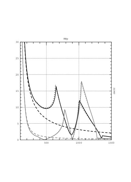
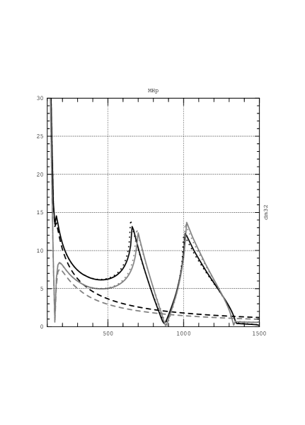
all sectors,   all sectors, $p^{2}=0$,   all sectors, $p^{2}=$ on-shell approx.

Figure 3.6: $\Delta m_{32}=m_{H_{3}}-m_{H_{2}}$ is shown as a function of $m_{H^{\pm}}$ for $\tan\beta=4$ (left) and $\tan\beta=15$ (right) for two different values of $\varphi_{A_{t}}$, $\varphi_{A_{t}}=\pi/2$ (black) and $\varphi_{A_{t}}=0$ (gray).

Chapter 4 Higgs boson production at the LC

Controlling the Higgs boson production properties at the per-cent level is mandatory to perform high-precision measurements at the LC. The Higgs boson production cross sections themselves will be measured at ${\cal O}(1\%)$ [37, 38]. In order to be able to exploit these measurements the experimental accuracy has to be matched with a corresponding theoretical precision. At the LC, the possible channels for neutral Higgs-boson production are the production via $Z$-boson exchange (Higgs-strahlung),

$$e^{+}e^{-} \to Z\to Z\{h,H\}\,,$$

$$e^{+}e^{-} \to Z\to A\{h,H\}\,,$$ (4.1)

and the $WW$-fusion channel,

$$e^{+}e^{-}\to\bar{\nu}_{e}W^{+}\;\nu_{e}W^{-}\to\bar{\nu}_{e}\nu_{e}\{h,H,A\}\,.$$ (4.2)

Charged Higgs bosons can be produced in pairs,

$$e^{+}e^{-}\to\{\gamma,Z\}\to H^{+}H^{-}$$ (4.3)

or singly,

$$e^{+}e^{-} \to \{\gamma,Z\}\to W^{+}H^{-}\,,$$ (4.4)

$$e^{+}e^{-} \to \bar{\nu}_{e}W^{+}\;e^{-}\{\gamma,Z\}\to\bar{\nu}_{e}e^{-}H^{+}$$ (4.5)

(and also with the charged conjugated processes). We do not discuss here the possibility of Higgs-particle production by bremsstrahlung off heavy quarks (e.g. $e^{+}e^{-}\to\bar{b}b\{h,H,A\}$, which can be significant for large $\tan\beta$ [81]).

The Higgs-strahlung processes, eq. (4.1), are possible at the tree-level. The full MSSM one-loop corrections can be found in Refs. [82, 83, 84]. The leading two-loop corrections have been incorporated in Ref. [85]. While the $WW$ fusion channel, eq. (4.2), for the ${\cal CP}$-even Higgs bosons are possible already at the tree-level [87, 86], the ${\cal CP}$-odd Higgs boson can only be produced at the loop level. Within the SM recently the full one-loop corrections to the $WW$ fusion channel have been obtained by two groups [88] (see also Ref. [89] for a partial analytical calculation). In the MSSM so far only the corrections from all [67] or third generation [90] fermion and sfermion loops are available. The ${\cal CP}$-odd channel has been evaluated including 3- and 4-point function one-loop corrections [91]. The pair production of the charged Higgs bosons, eq. (4.3), is possible at the tree-level, the full one-loop corrections in the MSSM can be found in Ref. [92]. The charged Higgs boson production in association with a $W$ boson, eq. (4.4), is mediated via loop diagrams, where the full one-loop corrections can be found in Refs. [93, 94]. Finally the single Higgs production in the gauge boson fusion channel, eq. (4.5), possible only at the loop level, has been evaluated including the full one-loop SM fermion and scalar fermion corrections in Ref. [95].

In the following subsections we will review the leading two-loop corrections to the Higgs-strahlung process, the (s)fermion one-loop corrections to the $WW$ fusion channel and the (s)fermion one-loop contribution to the single charged Higgs production in gauge boson fusion. The main phenomenological consequences are also discussed.

4.1 Corrections to the Higgs-strahlung channel

The most promising channels for the production of the ${\cal CP}$-even neutral MSSM Higgs bosons in the first phase of a LC are the Higgs-strahlung processes [86],

$$e^{+}e^{-}\to Z\,H_{i}~{},$$ (4.6)

($H_{1,2}=h,H$) and the associated production of a scalar and a pseudoscalar Higgs boson,

$$e^{+}e^{-}\to A\,H_{i}~{}.$$ (4.7)

We review the computation of the MSSM predictions for the cross sections of both channels in the Feynman-diagrammatic (FD) approach using the on-shell renormalization scheme. We take into account the complete set of one-loop contributions, thereby keeping the full dependence on all kinematical variables. The one-loop contributions consist of the corrections to the Higgs- and gauge-boson propagators, where the former contain the dominant electroweak one-loop corrections of ${\cal O}(\alpha_{t})$, and of the contributions to the 3-point and 4-point vertex functions [82, 83, 84]. We combine the complete one-loop result with the dominant two-loop QCD corrections of ${\cal O}(\alpha_{t}\alpha_{s})$ [16, 5] and further sub-dominant corrections. In this way the currently most accurate results for the cross sections are obtained.

Furthermore we show analytically that the Higgs-boson propagator corrections with neglected momentum dependence can be absorbed into the tree-level coupling using the effective mixing angle from the neutral ${\cal CP}$-even Higgs-boson sector. We compare our results for the cross sections with the approximation in which only the corrections to the effective mixing angle, evaluated within the renormalization-group-improved one-loop effective potential approach, are taken into account. For most parts of the MSSM parameter space we find agreement of the two approaches of better than 10% for the highest LEP energies, while for $\sqrt{s}=500\,\,\mathrm{GeV}$ the difference can reach 25%.

4.1.1 Cross sections for Higgs production in $e^{+}e^{-}$ collisions

Classification of radiative corrections

The set of diagrams taken into account for Higgs-strahlung $e^{+}e^{-}\to hZ$ is schematically shown in Fig. 4.1, where a) is the tree-level diagram. The shaded blobs summarize the loops with all possible virtual particles, except photons in the $Ze^{+}e^{-}$ vertex corrections, see above. More details can be found in Refs. [82, 83, 84]. An analogous set has been evaluated for the second process $e^{+}e^{-}\to hA$.

Figure 4.1: Generic one-loop diagrams contributing to the $e^{+}e^{-}\to Zh$ cross section.

For completeness, in Fig. 4.1 also contributions are shown that are proportional to the electron mass or vanish completely after contraction with the polarization vector of the $Z$ boson (e.g. the $A,G$–$Z$ mixing contributions and the longitudinal parts of the $Z$ and $\gamma$–$Z$ self-energies). The different types of corrections can be summarized as follows:

• Corrections to the $e$, $Z$, $\gamma$ and $\gamma$–$Z$ self-energies on the internal and external lines and to the (initial state) $Ze^{+}e^{-}$ and $\gamma e^{+}e^{-}$ vertices, b) – g).

• Corrections to the scalar and pseudoscalar propagators, h).

• Corrections to the $ZZH_{i}$ ($ZAH_{i}$) vertex, i).

• Box-diagram contributions and $t$-channel-exchange diagrams, j) – l).

The corrections (i)-(iv) have a different relative impact:

• Electroweak corrections of type (i) are typically of the order of a few percent (like in the Standard Model) and do not exhibit a strong dependence on any SUSY parameters.

• The main source of differences between the tree-level and higher-order results are the corrections to the Higgs-boson self-energies (ii). They are responsible for changes in the physical masses $M_{h}$ and $M_{H}$ and the effective mixing angle $\alpha_{\rm eff}$ (via contributions to the renormalization constants, ${\cal Z}^{\rm ext}$, for the external Higgs particles in the $S$-matrix elements, see Ref. [85]) predicted for given values of $\tan\beta$ and $M_{A}$. At the one-loop level these propagator corrections constitute the only source for the large correction of ${\cal O}(\alpha_{t})$. At the two-loop level they exclusively give rise to contributions of ${\cal O}(\alpha_{t}\alpha_{s})$ and of ${\cal O}(\alpha_{t}^{2})$. In this sense the propagator corrections define a closed subset of diagrams, being responsible for a numerically large contribution.

• Corrections to the final-state vertices (iii) are typically larger than those of type (i), but smaller than the Higgs-boson propagator corrections. At LEP2 energies they can reach at most 7–10% [82] for very low or very large values of $\tan\beta$, when the Yukawa couplings of the top or bottom quarks become strong.

• Finally, the box-diagram contributions (iv) depend strongly on the center-of-mass energy. They are of the order of 2–3% at LEP2 energies and may reach 20% for $\sqrt{s}=500$ GeV [84].

It should be noted that initial-state QED corrections as well as finite-width effects (allowing for off-shell decays of the Higgs and the $Z$ boson) are not included in our calculation. However, by incorporating our result into existing codes, e.g. HZHA [96], QED corrections and finite-width effects can be taken into account.

In Ref. [85] it has been shown analytically that the leading Higgs boson propagator corrections can be incorporated by changing the tree-level $\alpha$ in the Higgs–gauge boson couplings to $\alpha_{\rm eff}$, see also Sect. 5.1.2. For instance, for $Zh$ production, the Born coupling $\tilde{V}_{ZZh}\sim\sin(\alpha-\beta)\hskip 2.84526pt$ is changed by the leading propagator corrections to $\sin(\alpha_{\rm eff}-\beta)$. Analogous results hold for all Higgs vertices, including the $AH_{i}$ vertices. While the $\alpha_{\rm eff}$ approximation, i.e. using an improved Born result for the cross sections where the tree-level angle $\alpha$ is replaced by $\alpha_{\rm eff}$, incorporates the dominant one-loop and two-loop contributions, it is obvious from the discussion above that this approximation neglects many effects included in a full FD calculation. These are, in particular, the process-specific vertex and box corrections.

Cross sections

In this subsection we briefly summarize the analytical formulae for the cross sections for the on-shell production of the Higgs bosons $e^{+}e^{-}\to ZH_{i}$, $e^{+}e^{-}\to AH_{i}$ including the corrections (i)-(iii). Box diagrams (iv) give another, more complicated, set of formfactors that make the expressions quite lengthy and are, hence, omitted here; more details can be found in Ref. [83]. However, we include the box-diagram contributions, as described in Ref. [84], in our numerical programs [85] and in the figures shown in this section.

The presented formalism for cross sections is general enough to accommodate corrections of any order to 2- and 3-point vertex functions. Beyond the one-loop level, however, currently only two-loop corrections to the scalar propagators have been included [16, 5]. Therefore, in the cross section calculations we include all possible types of one-loop corrections and the available two-loop corrections to scalar self-energies. This is well justified because, as discussed above, propagator corrections constitute a closed subset of the leading ${\cal O}(\alpha_{t}\alpha_{s})$ and ${\cal O}(\alpha_{t}^{2})$ contributions. Therefore, these two-loop corrections are of particular relevance and interest.

The cross sections (in the center of mass system (CMS)) for both processes (4.6) and (4.7) have the form:

$${d\sigma_{Z(A)H_{i}}\over d\Omega}={\lambda\left(s,M^{2}_{Z(A)},M^{2}_{H_{i}}\right)\over 64\pi^{2}s^{2}\left|D_{Z}(s)\right|^{2}}\left({\cal A}_{1}+{\cal A}_{2}\cos^{2}\theta_{\rm CMS}\right),$$ (4.8)

where $\lambda$ is the standard phase space factor,

$$\lambda\left(s,m^{2}_{1},m^{2}_{2}\right)=\sqrt{s^{2}+m_{1}^{4}+m_{2}^{4}-2sm_{1}^{2}-2sm_{2}^{2}-2m^{2}_{1}m^{2}_{2}},$$ (4.9)

and ${\cal A}_{1},{\cal A}_{2}$ are defined by

$${\cal A}_{1}+{\cal A}_{2}\cos^{2}\theta_{\rm CMS}={1\over 4}\sum_{pol}\left({\cal M}{\cal M}^{*}\right),$$ (4.10)

with ${\cal M}_{ZS}$ and ${\cal M}_{PS}$ as given below. In the following, $\theta_{\rm CMS}$ denotes the scattering angle $\theta_{\rm CMS}=<)\,(e^{-},H_{i})$ in the CMS. The momenta of the incoming electron and positron are denoted as $k_{1}$ and $k_{2}$, respectively. The momentum of the outgoing $h/H$ is labeled with $q$, whereas the outgoing $Z/A$ momentum is denoted as $p$, see Fig. 4.1a. The matrix elements for the Higgs-strahlung process and the associated Higgs production read

$${\cal M}_{ZS}^{i} = e\overline{v}(k_{2})\gamma^{\nu}\left[\tilde{V}^{\mu\nu i}_{ZZS}\left(\hat{c}_{V}-\hat{c}_{A}\gamma^{5}\right)+{\tilde{V}}^{\mu\nu i}_{\gamma ZS}{D_{Z}(s)\over D_{\gamma}(s)}-\tilde{V}^{(0)\mu\nu i}_{ZZS}{\hat{\Sigma}^{T}_{\gamma Z}(s)\over D_{\gamma}(s)}\right]u(k_{1})\epsilon_{\mu}(p)$$ (4.11)

$$+{\rm~{}box~{}corrections},$$

$${\cal M}_{PS}^{i} = e\overline{v}(k_{2})\gamma_{\mu}\left[\tilde{V}^{\mu ij}_{ZPS}\left(\hat{c}_{V}-\hat{c}_{A}\gamma^{5}\right)+{\tilde{V}}^{\mu ij}_{\gamma PS}{D_{Z}(s)\over D_{\gamma}(s)}-\tilde{V}^{(0)\mu ij}_{ZPS}{\hat{\Sigma}^{T}_{\gamma Z}(s)\over D_{\gamma}(s)}\right]u(k_{1})$$ (4.12)

$$+{\rm~{}box~{}corrections}.$$

For the corresponding expressions for the box contributions see Ref. [83].

In the above expressions $u(k_{1})$ and $v(k_{2})$ are spinors of the incoming electron-positron pair, $\epsilon_{\mu}(p)$ is the polarization vector of the outgoing $Z$. $\hat{c}_{V},\hat{c}_{A}$ are the renormalized vector and axial couplings of the $Z$ boson to an electron-positron pair, at the one-loop level $\hat{c}_{A}=-1/4s_{W}c_{W}+\hat{c}_{A}^{(1)}$, $\hat{c}_{V}=\left(-1+4s^{2}_{W}\right)/4s_{W}c_{W}+\hat{c}_{V}^{(1)}$, $c_{\mathrm{w}}^{2}\equiv 1-s_{\mathrm{w}}^{2}\equiv M_{W}^{2}/M_{Z}^{2}$. $\hat{\Sigma}^{T}_{Z}(s)$, $\hat{\Sigma}_{\gamma}(s)$ and $\hat{\Sigma}^{T}_{\gamma Z}(s)$ denote the renormalized photon and transverse $Z$ boson self-energies. $D_{Z}(s)$ and $D_{\gamma}(s)$ are the inverse $Z$ and photon propagators defined as

$$D_{Z}(s)=s-M_{Z}^{2}+\hat{\Sigma}^{T}_{Z}(s)~{},$$

$$D_{\gamma}(s)=s+\hat{\Sigma}_{\gamma}(s)~{}.$$ (4.13)

Finally, $\tilde{V}$ denotes the effective neutral Higgs–gauge-boson vertices with the one-loop form factors. The explicit expression for those vertices and for the matrix elements for Higgs-strahlung and associated Higgs production can be found in the Appendix of Ref. [85] and in Ref. [82].

4.1.2 Numerical results

In the following we present numerical examples for the dependence of the neutral Higgs-boson couplings and cross sections on $\tan\beta$, $M_{h}$, and the mixing in the scalar top sector. The results are obtained in the $m_{h}^{\rm max}$ and the no-mixing scenario [53], see the Appendix. Only for the scalar soft SUSY-breaking parameters we have set the slepton mass parameters to $M_{\tilde{l}}=300\,\,\mathrm{GeV}$. The squark mass parameter is denoted as $M_{\tilde{q}}$.

Below we will also perform comparisons with results obtained in the framework of the RG improved one-loop EPA, where the input parameters are understood as $\overline{\rm{MS}}$ quantities. To ensure consistency, in the latter case we have transformed the on-shell SUSY input parameters into the corresponding $\overline{\rm{MS}}$ values as discussed in Ref. [59]. The results shown below for the higher-order corrected Higgs-boson masses and the mixing angle within the RG improved one-loop EPA have been obtained with the Fortran program subhpole (based on Refs. [14, 59]).

Differences in the Higgs-production cross sections between our FD result (containing the complete one-loop result and the dominant two-loop corrections) and the RG $\alpha_{\rm eff}$ approximation have a two-fold origin: the different predictions for the values of $M_{h}$ and $\alpha_{\rm eff}$, and the additional contributions contained in the FD result (i.e. the one-loop 3- and 4-point vertex functions.

Figure 4.2: $\sigma_{Zh}$ and $\sigma_{Ah}$ as a function of $M_{h}$ at $\sqrt{s}=500\,\,\mathrm{GeV}$, for two values of $M_{A}$, in the $m_{h}^{\rm max}$ scenario. The solid (dot-dashed) line represents the two-loop FD result including (excluding) box contributions, the dotted line shows the RG $\alpha_{\rm eff}$ approximation and the dashed line shows the one-loop FD result.

Figure 4.3: $\sigma_{Zh}$ and $\sigma_{Ah}$ as a function of $\sqrt{s}$ for $\tan\beta=5$, in the no-mixing scenario. The solid (dot-dashed) line represents the two-loop FD result including (excluding) box contributions, the dotted line shows the RG $\alpha_{\rm eff}$ approximation and the dashed line shows the one-loop FD result.

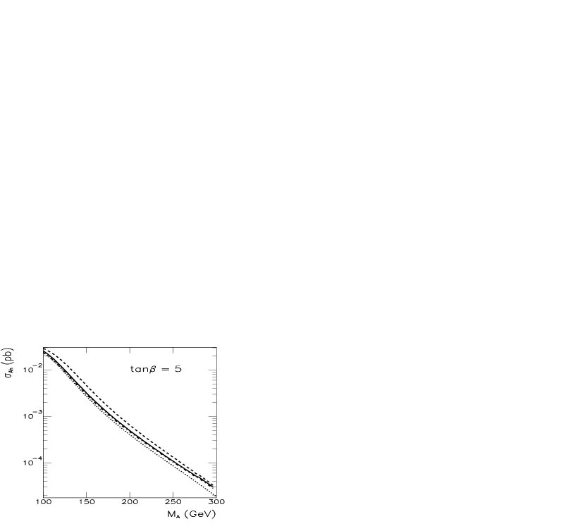
Figure 4.4: $\sigma_{Zh}$ and $\sigma_{Ah}$ as a function of $M_{A}$ at $\sqrt{s}=500\,\,\mathrm{GeV}$, shown for $\tan\beta=5$ and $\tan\beta=50$, in the no-mixing scenario. The solid (dot-dashed) line represents the two-loop FD result including (excluding) box contributions, the dotted line shows the RG $\alpha_{\rm eff}$ approximation and the dashed line shows the one-loop FD result.

In Fig. 4.2 the cross sections for the Higgs-strahlung process and the associated production are shown for a typical Linear Collider energy, $\sqrt{s}=500$ GeV [37], in the $m_{h}^{\rm max}$ scenario (in the no-mixing scenario similar results have been obtained). We also show the result for the two-loop FD calculation where the box contributions have not been included, in order to point out their relative importance for high-energy collisions. For $\sqrt{s}=500\,\,\mathrm{GeV}$ the differences between the FD result and the RG $\alpha_{\rm eff}$ approximation can be large, an effect that is more pronounced for the higher value of $M_{A}$. For $M_{A}=200\,\,\mathrm{GeV}$, typically they are of the order of 10–15% for $\sigma_{Zh}$ and even up to 25% for $\sigma_{Ah}$ (for $M_{h}\;\raisebox{-3.00003pt}{$\stackrel{{\scriptstyle\displaystyle>}}{{\sim}}$}\;90\,\,\mathrm{GeV}$). The difference between the two-loop and one-loop FD result can be sizable. The two-loop result for $\sigma_{Zh}$ is in general larger than the one-loop value, again increasing with $M_{A}$, where for $M_{A}=200\,\,\mathrm{GeV}$ the difference can amount up to 15%. $\sigma_{Ah}$, on the other hand, is decreased at the two-loop level for $M_{A}=200\,\,\mathrm{GeV}$ and the difference may be sizable.

The box contributions become more important for higher $\sqrt{s}$ and change the total cross section by 5–10%. This result remains unchanged even if sleptons are significantly heavier than $M_{\tilde{l}}=300$ GeV used in our numerical analysis, as the dominant contributions to box diagrams are given by $W$ and Higgs boson exchanges [83, 84], which do not depend on $M_{\tilde{l}}$. Also, one should recall that box contributions lead to an angular distribution of the final-state particles different from the effective Born approximation and thus give much larger corrections to the differential rather than to the total cross section, at least for some range of the scattering angle. Therefore, the box diagrams have a significant effect at Linear Collider energies and thus have to be included. The same conclusions can be drawn for $\sqrt{s}=500\,\,\mathrm{GeV}$ in the no-mixing scenario, which we do not show here. The differences between the FD result and the RG $\alpha_{\rm eff}$ approximation are only slightly smaller than in the $m_{h}^{\rm max}$ case.

In Fig. 4.3 the results for $\sigma_{Zh}$ and $\sigma_{Ah}$ are shown as a function of $\sqrt{s}$ in the no-mixing scenario for $M_{A}=100,200\,\,\mathrm{GeV}$. Besides the obvious kinematical drop-off of the cross sections, one can observe that the relative differences between the FD two-loop result and the RG $\alpha_{\rm eff}$ approximation grow with $\sqrt{s}$. The differences remain almost constant or even increase slowly in absolute terms, whereas the full cross sections decrease. $\sigma_{Ah}$ becomes very small for large $M_{A}$, as can be seen in more detail in Fig. 4.4. There we show the dependence of $\sigma_{Zh}$ and $\sigma_{Ah}$ on $M_{A}$ in the no-mixing scenario for $\tan\beta=5$ and $\tan\beta=50$. For $\sigma_{Zh}$, the $A$ boson decouples quickly; the dependence on $M_{A}$ becomes very weak for $M_{A}\;\raisebox{-3.00003pt}{$\stackrel{{\scriptstyle\displaystyle>}}{{\sim}}$}\;250\,\,\mathrm{GeV}$, when $\sigma_{Zh}$ is already practically constant (compare e.g. Ref. [5]). In the same limit, $\sigma_{Ah}$ goes quickly to zero due to suppression of the effective $ZhA$ coupling, which is $\sim\cos(\alpha_{\rm eff}-\beta)$; also the kinematical suppression plays a role, but this becomes significant only for sufficiently large $M_{A}$, $M_{A}>350\,\,\mathrm{GeV}$. For large $\tan\beta$ the decoupling of $M_{A}$ is even more rapid. The differences between the FD two-loop result and the RG $\alpha_{\rm eff}$ approximation for the Higgs-strahlung cross section tend also to a constant, but they increase with $M_{A}$ for the associated production. The latter can be explained by the growing relative importance of 3- and 4-point vertex function contributions compared to the strongly suppressed Born-like diagrams. As can be seen from Fig. 4.4, for $\tan\beta=50$ and $M_{A}\geq 300\,\,\mathrm{GeV}$ the FD two-loop result is almost an order of magnitude larger than the result of the RG $\alpha_{\rm eff}$ approximation, and starts to saturate. This can be attributed to the fact that the (non-decoupling) vertex and box contributions begin to dominate the cross section value. However, such a situation occurs only for very small $\sigma_{Ah}$ values, $\sigma_{Ah}\approx 10^{-3}$ fb, below the expected experimental LC sensitivities.

4.2 Corrections to the $WW$ fusion channel

While the discovery of one light Higgs boson might well be compatible with the predictions both of the SM and the MSSM, the discovery of one or more other heavy Higgs bosons would be a clear and unambiguous signal for physics beyond the SM.

In the decoupling limit, i.e. for $M_{A}\;\raisebox{-3.00003pt}{$\stackrel{{\scriptstyle\displaystyle>}}{{\sim}}$}\;200\,\,\mathrm{GeV}$, the heavy MSSM Higgs bosons are nearly degenerate in mass, $M_{A}\sim M_{H}\sim M_{H^{\pm}}$. The couplings of the neutral Higgs bosons to SM gauge bosons are proportional to

$$VVh \sim VHA\sim\sin(\beta-\alpha)\hskip 2.84526pt\,,$$ (4.14)

$$VVH \sim VhA\sim\cos(\beta-\alpha)\hskip 2.84526pt\,,\qquad(V=Z,W^{\pm})~{}.$$ (4.15)

In the decoupling limit one finds $\beta-\alpha\to\pi/2$, i.e. $\sin(\beta-\alpha)\hskip 2.84526pt\to 1$, $\cos(\beta-\alpha)\hskip 2.84526pt\to 0$.

At the LC, the possible channels for neutral Higgs-boson production are the production via $Z$-boson exchange, eq. (4.1), and the $WW$ fusion channel, eq. (4.2). As a consequence of the coupling structure, in the decoupling limit the heavy Higgs boson can only be produced in $(H,A)$ pairs. This limits the LC reach to $M_{H}\;\raisebox{-3.00003pt}{$\stackrel{{\scriptstyle\displaystyle<}}{{\sim}}$}\;\sqrt{s}/2$. Higher-order corrections to the $WW\to H$ channel from loops of fermions and sfermions, however, involve potentially large contributions from the top and bottom Yukawa couplings and could thus significantly affect the decoupling behavior.

In this section we review the one-loop corrections of fermions and sfermions to the process $e^{+}e^{-}\to\bar{\nu}\nu\,\{h,H\}$, i.e. to the production of a neutral ${\cal CP}$-even Higgs boson in association with a neutrino pair, both via the $WW$-fusion and the Higgs-strahlung mechanism. In the latter case the $Z$ boson is connected to a neutrino pair, $e^{+}e^{-}\to Z\{h,H\}\to\bar{\nu}_{l}\nu_{l}\{h,H\}$, with $l=e,\mu,\tau$ (where the latter two neutrinos result in an indistinguishable final state in the detector).

While the well-known universal Higgs-boson propagator corrections turned out not to significantly modify the decoupling behavior of the heavy ${\cal CP}$-even Higgs boson, an analysis of the process-specific contributions to the $WWH$ vertex has been obtained recently. Taking into account all loop and counter-term contributions to the process $e^{+}e^{-}\to\bar{\nu}\nu\,\{h,H\}$ from fermions and sfermions and including also the effects of beam polarization in our analysis, we review in this section the LC reach for the heavy ${\cal CP}$-even Higgs boson. We have obtained results for values of the MSSM parameters according to the four benchmark scenarios defined in Ref. [53]. While within these benchmark scenarios we find that the loop corrections do not significantly enhance the LC reach for heavy ${\cal CP}$-even Higgs boson production and in some cases even slightly reduce the accessible parameter space, we have also investigated MSSM parameter regions where the loop effects do in fact lead to a significant improvement of the LC reach. In “favorable” MSSM parameter regions an $e^{+}e^{-}$ LC running at $\sqrt{s}=1\,\,\mathrm{TeV}$ can be capable of producing a heavy ${\cal CP}$-even Higgs boson with a mass up to $M_{H}\;\raisebox{-3.00003pt}{$\stackrel{{\scriptstyle\displaystyle<}}{{\sim}}$}\;700\,\,\mathrm{GeV}$.

Concerning the production of the light ${\cal CP}$-even Higgs boson, an accurate prediction of the production cross section for precision analyses will be necessary. Aiming for analyses at the percent level [38] also requires a prediction of the production cross section in this range of precision. Besides the already known universal Higgs propagator corrections, in particular loops from fermions and sfermions (especially from the third family) are expected to give relevant contributions. We analyze our results for the parameters of the four benchmark scenarios defined in Ref. [53] and study the results as a function of different SUSY parameters. We discuss the relative importance of the fermion- and the sfermion-loop contributions and furthermore evaluate the fermion-loop correction within the SM for comparison purposes (the complete ${\cal O}(\alpha)$ corrections within the SM can be found in Ref. [88]).

4.2.1 Renormalization in the Higgs sector

The renormalized Higgs-boson self-energies, see eqs. (3.49a)-(3.49c), are as usual given by

$$\hat{\Sigma}_{HH}(q^{2}) = \Sigma_{HH}(q^{2})+\delta Z_{H}(q^{2}-m_{H}^{2})-\delta m_{H}^{2}\,,$$

$$\hat{\Sigma}_{hH}(q^{2}) = \Sigma_{hH}(q^{2})+\frac{1}{2}\delta Z_{Hh}(q^{2}-m_{H}^{2})+\frac{1}{2}\delta Z_{hH}(q^{2}-m_{h}^{2})-\delta m_{hH}^{2}\,,$$

$$\hat{\Sigma}_{hh}(q^{2}) = \Sigma_{hh}(q^{2})+\delta Z_{h}(q^{2}-m_{h}^{2})-\delta m_{h}^{2}\,.$$ (4.16)

The mass counter terms arise from the renormalization of the Higgs potential, see Ref. [51]. They are evaluated in the on-shell renormalization scheme. The field-renormalization constants, see also eq. (3.57) can be obtained in the $\overline{\rm{DR}}$ scheme, leading to

$$\delta Z_{H} = -\left[\mbox{Re}\,\Sigma_{HH}^{\prime}(m_{H}^{2})\right]^{\rm div},$$

$$\delta Z_{h} = -\left[\mbox{Re}\,\Sigma_{hh}^{\prime}(m_{h}^{2})\right]^{\rm div},$$

$$\delta Z_{hH} = \frac{\sin\alpha\hskip 2.84526pt\cos\alpha\hskip 2.84526pt}{\cos 2\alpha\hskip 2.84526pt}(\delta Z_{h}-\delta Z_{H})\,,$$

$$\delta Z_{Hh} = \delta Z_{hH}\,,$$ (4.17)

i.e. only the divergent parts of the renormalization constants in eqs. (4.17) are taken into account. As renormalization scale we have chosen $\mu_{\overline{\rm{DR}}}=m_{t}$. The finite LSZ factors required in this renormalization scheme are described in the next subsection.

4.2.2 The process $e^{+}e^{-}\to\bar{\nu}_{e}\nu_{e}\,\{h,H\}$

The tree-level process

The tree-level process [87, 86] consists of the two diagrams shown in Fig. 4.5. Besides the $WW$-fusion contribution (left diagram), we also take into account the Higgs-strahlung contribution (right diagram), where a virtual $Z$ boson is connected to two electron neutrinos.

Figure 4.5: The tree-level diagrams for the process $e^{+}e^{-}\to\bar{\nu}\nu\,\{h,H\}$, consisting of the $WW$-fusion contribution (left) and the Higgs-strahlung contribution (right).

An analytical expression for the tree-level cross section for a SM Higgs boson can be found e.g. in Ref. [97]. For relatively low energies and moderate values of the SM Higgs-boson mass ($\sqrt{s}\;\raisebox{-3.00003pt}{$\stackrel{{\scriptstyle\displaystyle<}}{{\sim}}$}\;400\,\,\mathrm{GeV}$, $M_{H_{\rm SM}}\;\raisebox{-3.00003pt}{$\stackrel{{\scriptstyle\displaystyle<}}{{\sim}}$}\;200\,\,\mathrm{GeV}$) the resonant production via the Higgs-strahlung contribution dominates over the $WW$-fusion contribution. At higher energies, however, the $WW$-fusion contribution becomes dominant. The cross section, containing both contributions, in the high-energy limit takes the simple form [86]

$$\sigma(e^{+}e^{-}\to\bar{\nu}_{e}\nu_{e}H_{\rm SM})\to\frac{G_{F}^{3}M_{W}^{4}}{4\sqrt{2}\,\pi^{3}}\left[\left(1+\frac{M_{H_{\rm SM}}^{2}}{s}\right)\log\left(\frac{s}{M_{H_{\rm SM}}^{2}}\right)-2\left(1-\frac{M_{H_{\rm SM}}^{2}}{s}\right)\right],$$ (4.18)

where the $t$-channel contribution from the $WW$-fusion diagram gives rise to the logarithmic increase.

The coefficients for the couplings $WWh$ and $WWH$ are denoted by $\Gamma_{h}^{(0)}$ and $\Gamma_{H}^{(0)}$ at the tree level, respectively (and analogously for the $ZZh$ and $ZZH$ couplings):

$$\Gamma_{h}^{(0)} = \frac{\mathrm{i}\,e\,M_{W}}{s_{\mathrm{w}}}\sin(\beta-\alpha)\hskip 2.84526pt\,,$$ (4.19)

$$\Gamma_{H}^{(0)} = \frac{\mathrm{i}\,e\,M_{W}}{s_{\mathrm{w}}}\cos(\beta-\alpha)\hskip 2.84526pt\,.$$ (4.20)

The SM coupling $\Gamma^{(0)}_{H_{\rm SM}}$ is obtained by dropping the SUSY factors $\sin(\beta-\alpha)\hskip 2.84526pt$ or $\cos(\beta-\alpha)\hskip 2.84526pt$. In the decoupling limit, $M_{A}\;\raisebox{-3.00003pt}{$\stackrel{{\scriptstyle\displaystyle>}}{{\sim}}$}\;200\,\,\mathrm{GeV}$, $\beta-\alpha\to\pi/2$, so that $\sin(\beta-\alpha)\hskip 2.84526pt\to 1$ and $\cos(\beta-\alpha)\hskip 2.84526pt\to 0$, i.e. the heavy neutral ${\cal CP}$-even Higgs boson decouples from the $W$ and $Z$ bosons.

We parametrize the Born matrix element by the Fermi constant, $G_{F}$, i.e. we use the relation

$$e=2\;s_{\mathrm{w}}\;M_{W}\left[\frac{\sqrt{2}\,G_{F}}{1+\Delta r}\right]^{1/2},$$ (4.21)

where $\Delta r$ incorporates higher-order corrections, see the next subsection.

Higher-order corrections

In the description of our calculation below we will mainly concentrate on the $WW$-fusion contribution. The Higgs-strahlung contribution, which we describe in less detail, is taken into account in exactly the same way (with the only exception that a finite $Z$ width has to be taken into account).

We evaluate the one-loop ${\cal O}(\alpha)$ contributions from loops involving all fermions and sfermions. Especially the corrections involving third-generation fermions and sfermions, i.e. $t,b,\tau,\nu_{\tau}$, and their corresponding superpartners, $\tilde{t}_{1},\tilde{t}_{2}$, $\tilde{b}_{1},\tilde{b}_{2}$, $\tilde{\tau}_{1},\tilde{\tau}_{2}$, $\tilde{\nu}_{\tau}$, are expected to be sizable, since they contain potentially large Yukawa couplings, $y_{t}$, $y_{b}$, $y_{\tau}$, where the down-type couplings can be enhanced in the MSSM for large values of $\tan\beta$. This class of diagrams in particular contains contributions enhanced by $m_{t}^{2}/M_{W}^{2}$.

The contributions involve corrections to the $WW\{h,H\}$ vertex and the corresponding counter-term diagram, shown in Fig. 4.6, corrections to the $W$-boson propagators and the corresponding counter terms, shown in Fig. 4.7, and the counter-term contributions to the $e\nu_{e}W$ vertex as shown in Fig. 4.8. Furthermore, Higgs propagator corrections enter via the wave-function normalization of the external Higgs boson, see below. There are also $W$-boson propagator corrections inducing a transition from the $W^{\pm}$ to either $G^{\pm}$ or $H^{\pm}$. These corrections affect only the longitudinal part of the $W$ boson, however, and are thus $\propto m_{e}/M_{W}$ and have been neglected.

Figure 4.6: Corrections to the $WW\{h,H\}$ vertex and the corresponding counter-term diagram. The label $\hbox to0.0pt{\raise 7.22223pt\hbox{\tiny${}_{\,(\;\,)}$}\hss}\tilde{f}$ denotes all (s)fermions, except in the presence of a $\hbox to0.0pt{\raise 7.22223pt\hbox{\tiny${}_{\,(\;\,)}$}\hss}\tilde{f}\,^{\prime}$, in which case the former denotes only the isospin-up and the latter the isospin-down members of the (s)fermion doublets.

Figure 4.7: Corrections to the $W$-boson propagator and the corresponding counter-term diagrams. The label $\hbox to0.0pt{\raise 7.22223pt\hbox{\tiny${}_{\,(\;\,)}$}\hss}\tilde{f}$ denotes all (s)fermions, except in the presence of a $\hbox to0.0pt{\raise 7.22223pt\hbox{\tiny${}_{\,(\;\,)}$}\hss}\tilde{f}\,^{\prime}$, in which case the former denotes only the isospin-up and the latter the isospin-down members of the (s)fermion doublets.

Figure 4.8: Counter-term contributions entering via the $e\,\nu_{e}\,W$ vertex.

While the renormalization in the counter terms depicted in Figs. 4.7 and 4.8 is as in the SM (see e.g. Ref. [98]), the $WW\{h,H\}$ vertices are renormalized as follows,

$$WWh:\,\Gamma_{WWh}^{(0),{\rm CT}}=\Gamma_{h}^{(0)} \Biggl{[}1+\delta\tilde{Z}_{e}+\frac{1}{2}\frac{\delta M_{W}^{2}}{M_{W}^{2}}+\delta Z_{W}+\frac{\delta s_{\mathrm{w}}}{s_{\mathrm{w}}}$$

$${}+\sin\beta\,\cos\beta\hskip 2.84526pt\frac{\cos(\beta-\alpha)\hskip 2.84526pt}{\sin(\beta-\alpha)\hskip 2.84526pt}\delta\tan\beta+\frac{1}{2}\delta Z_{h}+\frac{1}{2}\frac{\Gamma_{H}^{(0)}}{\Gamma_{h}^{(0)}}\delta Z_{Hh}\Biggr{]}$$

$$WWH:\,\Gamma_{WWH}^{(0),{\rm CT}}=\Gamma_{H}^{(0)} \Biggl{[}1+\delta\tilde{Z}_{e}+\frac{1}{2}\frac{\delta M_{W}^{2}}{M_{W}^{2}}+\delta Z_{W}+\frac{\delta s_{\mathrm{w}}}{s_{\mathrm{w}}}$$

$${}-\sin\beta\,\cos\beta\hskip 2.84526pt\frac{\sin(\beta-\alpha)\hskip 2.84526pt}{\cos(\beta-\alpha)\hskip 2.84526pt}\delta\tan\beta+\frac{1}{2}\delta Z_{H}+\frac{1}{2}\frac{\Gamma_{h}^{(0)}}{\Gamma_{H}^{(0)}}\delta Z_{hH}\Biggr{]}$$

Analogous expressions are obtained for $\Gamma_{ZZ\Phi}^{(0),{\rm CT}}$ ($\Phi=h,H$). In the above expressions $\delta\tilde{Z}_{e}$ incorporates the charge renormalization and the $\Delta r$ contribution arising from eq. (4.21),

$$\delta\tilde{Z}_{e}=\delta Z_{e}-\frac{1}{2}\Delta r,\quad\delta Z_{e}=\frac{1}{2}\Pi^{\gamma}(0)-\frac{s_{\mathrm{w}}}{c_{\mathrm{w}}}\frac{\Sigma_{\gamma Z}^{T}(0)}{M_{Z}^{2}}\,,$$ (4.24)

where $\Sigma^{T}$ denotes the transverse part of a self-energy. $\delta M_{W}^{2}$ is the $W$-mass counter term, $\delta Z_{W}$ is the corresponding field-renormalization constant, and $\delta s_{\mathrm{w}}$ denotes the renormalization constant for the weak mixing angle. The field-renormalization constants, $\delta Z_{H},\delta Z_{h}$, and $\delta Z_{Hh}=\delta Z_{hH}$ are given in eq. (4.17). The counter term for $\tan\beta$ (with $\tan\beta\to\tan\beta(1+\delta\tan\beta)$) is derived in the $\overline{\rm{DR}}$ renormalization scheme [51] (using DRED). The parameter $\tan\beta$ in our result thus corresponds to the $\overline{\rm{DR}}$ parameter, taken at the scale $\mu_{\overline{\rm{DR}}}=m_{t}$. We list here all contributing counter terms except for the Higgs field renormalization which has already been given in eq. (4.17):

$$\delta M_{W}^{2} = \mbox{Re}\,\Sigma_{W}^{T}(M_{W}^{2})\,,$$ (4.25)

$$\delta M_{Z}^{2} = \mbox{Re}\,\Sigma_{Z}^{T}(M_{Z}^{2})\,,$$ (4.26)

$$\frac{\delta s_{\mathrm{w}}}{s_{\mathrm{w}}} = \frac{1}{2}\frac{c_{\mathrm{w}}^{2}}{s_{\mathrm{w}}^{2}}\left(\frac{\delta M_{Z}^{2}}{M_{Z}^{2}}-\frac{\delta M_{W}^{2}}{M_{W}^{2}}\right),$$ (4.27)

$$\delta\tan\beta = \delta\tan\beta^{\overline{\rm{DR}}}=-\frac{1}{2\cos 2\alpha\hskip 2.84526pt}\left[\mbox{Re}\,\Sigma_{hh}^{\prime}(m_{h}^{2})-\mbox{Re}\,\Sigma_{HH}^{\prime}(m_{H}^{2})\right]^{\rm div}.$$ (4.28)

For $\delta\tilde{Z}_{e}$ we find, taking into account only contributions from fermion and sfermion loops,

$$\delta\tilde{Z}_{e}=\frac{1}{2}\left\{\frac{c_{\mathrm{w}}^{2}}{s_{\mathrm{w}}^{2}}\left(\frac{\delta M_{Z}^{2}}{M_{Z}^{2}}-\frac{\delta M_{W}^{2}}{M_{W}^{2}}\right)-\left[\frac{\Sigma_{W}^{T}(0)-\delta M_{W}^{2}}{M_{W}^{2}}\right]\right\}\,.$$ (4.29)

The gauge-boson field-renormalization constants, $\delta Z_{W},\delta Z_{Z},\delta Z_{\gamma Z}$, drop out in the result for the complete $S$-matrix element.

In order to ensure the correct on-shell properties of the outgoing Higgs boson, which are necessary for the correct renormalization of the $S$-matrix element, furthermore finite wave-function normalizations have to be incorporated, see below. For the various checks that have been performed to ensure the reliability of our result, see Ref. [67].

The individual contributions from fermions and sfermions constitute two subsets of the full result which are individually UV-finite. This is in contrast to the evaluation of renormalized Higgs boson self-energies (see e.g. Refs. [10, 11]), where a UV-finite result is obtained only after adding the fermion- and sfermion-loop contributions.

The Higgs-boson propagator corrections and the effective Born approximation

For the correct normalization of the $S$-matrix element, finite Higgs-boson propagator corrections have to be included such that the residues of the outgoing Higgs bosons are set to unity and no mixing between $h$ and $H$ occurs on the mass shell of the two particles. The corrections affecting the Higgs-boson propagators and the Higgs-boson masses are numerically very important. Therefore we go beyond the one-loop fermion/sfermion contribution used for the evaluation of the genuine one-loop diagrams and include Higgs-boson corrections also from other sectors of the model [10, 11] as well as the dominant two-loop contributions [5, 7] as incorporated in the program FeynHiggs [48].

For the $WW\{h,H\}$ vertex, these contributions can be included as follows, yielding the correct normalization of the $S$ matrix at one-loop order:

$$WWh : \quad\sqrt{\hat{Z}_{h}}\left(\Gamma_{h}^{(0)}+\frac{1}{2}\hat{Z}_{Hh}\;\Gamma_{H}^{(0)}\right),$$ (4.30)

$$WWH : \quad\sqrt{\hat{Z}_{H}}\left(\Gamma_{H}^{(0)}+\frac{1}{2}\hat{Z}_{hH}\;\Gamma_{h}^{(0)}\right)\,.$$ (4.31)

This gives rise to the following terms:

$$WWh:\quad\Gamma_{WWh}^{{\rm WF}} = \Gamma_{h}^{(0)}\;\Biggl{[}\left(\sqrt{\hat{Z}_{h}}-1\right)+\frac{1}{2}\frac{\Gamma_{H}^{(0)}}{\Gamma_{h}^{(0)}}\sqrt{\hat{Z}_{h}}\;\hat{Z}_{Hh}\Biggr{]}\,,$$ (4.32)

$$WWH:\quad\Gamma_{WWH}^{{\rm WF}} = \Gamma_{H}^{(0)}\;\Biggl{[}\left(\sqrt{\hat{Z}_{H}}-1\right)+\frac{1}{2}\frac{\Gamma_{h}^{(0)}}{\Gamma_{H}^{(0)}}\sqrt{\hat{Z}_{H}}\;\hat{Z}_{hH}\Biggr{]}\,.$$ (4.33)

Analogous expressions are obtained for $\Gamma_{ZZ\Phi}^{\rm WF}$ ($\Phi=h,H$). In the above expressions, the finite Higgs-mixing contributions enter,

$$\hat{Z}_{Hh} = -2\;\frac{\mbox{Re}\,\hat{\Sigma}_{hH}(M_{h}^{2})}{M_{h}^{2}-m_{H}^{2}+\mbox{Re}\,\hat{\Sigma}_{HH}(M_{h}^{2})}\,,$$ (4.34)

$$\hat{Z}_{hH} = -2\;\frac{\mbox{Re}\,\hat{\Sigma}_{hH}(M_{H}^{2})}{M_{H}^{2}-m_{h}^{2}+\mbox{Re}\,\hat{\Sigma}_{hh}(M_{H}^{2})}\,,$$ (4.35)

involving the renormalized self-energies $\hat{\Sigma}(q^{2})$, see eq. (4.16), which contain corrections up to the two-loop level. The wave-function normalization factors $\hat{Z}_{h},\hat{Z}_{H}$ are related to the finite residue of the Higgs-boson propagators:

$$\hat{Z}_{h} = \frac{1}{1+\mbox{Re}\,\hat{\Sigma}^{\prime}_{hh}(q^{2})-\left(\frac{\left(\mbox{Re}\,\hat{\Sigma}_{hH}(q^{2})\right)^{2}}{q^{2}-m_{H}^{2}+\mbox{Re}\,\hat{\Sigma}_{HH}(q^{2})}\right)^{\prime}}~{}_{\Bigr{|}q^{2}=M_{h}^{2}}\,,$$ (4.36)

$$\hat{Z}_{H} = \frac{1}{1+\mbox{Re}\,\hat{\Sigma}^{\prime}_{HH}(q^{2})-\left(\frac{\left(\mbox{Re}\,\hat{\Sigma}_{hH}(q^{2})\right)^{2}}{q^{2}-m_{h}^{2}+\mbox{Re}\,\hat{\Sigma}_{hh}(q^{2})}\right)^{\prime}}~{}_{\Bigr{|}q^{2}=M_{H}^{2}}\,.$$ (4.37)

^′ denotes the derivative with respect to the momentum squared.

If in eqs. (4.34)–(4.37) the renormalized self-energies were evaluated at $q^{2}=0$, the above wave-function correction would reduce to the $\alpha_{\rm eff}$ approximation [99, 85]. In this approximation, however, the outgoing Higgs boson does not have the correct on-shell properties.

In order to analyze the effect of those corrections that go beyond the universal Higgs propagator corrections, we include the Higgs propagator corrections according to eqs. (4.32)–(4.37) into our Born matrix element, see the next subsection. Concerning our numerical analysis, see Sect. 4.2.2, we either use this Born cross section (thus the difference between our tree-level and the one-loop cross sections indicates the effect of the new genuine loop corrections), or we use the $\alpha_{\rm eff}$ approximation (so that the difference between the tree-level and the one-loop cross section directly shows the effect of our new calculation compared to the previously used results).

The higher-order production cross section

The amplitude for the process $e^{+}e^{-}\to\bar{\nu}_{e}\nu_{e}\,\{h,H\}$ is denoted as

$${\cal M}^{(i)}_{\Phi,e},\quad(\Phi=h,H;\ i=0,1)\,,$$ (4.38)

where $i=0$ denotes the lowest-order contribution and $i=1$ the one-loop correction.

The tree-level amplitude involves the $WW$-fusion channel (left diagram of Fig. 4.5) and the Higgs-strahlung process (right diagram of Fig. 4.5) where the virtual $Z$ boson is connected to two electron neutrinos. As explained above, we include the Higgs propagator corrections into our lowest-order matrix element. We use

$${\cal M}^{(0)}_{\Phi,e}={\cal M}^{\rm tree}_{\Phi,e}+{\cal M}^{\rm WF}_{\Phi,e}\,,$$ (4.39)

where ${\cal M}^{\rm tree}_{\Phi,e}$ is the contribution of the two tree-level diagrams, parametrized with $\alpha=\alpha_{\rm tree}$, eq. (2.33), and ${\cal M}^{\rm WF}_{\Phi,e}$ denotes the wave-function normalization contributions given in eqs. (4.32)–(4.37) (and analogously for the $ZZ\{h,H\}$ vertices).

At one-loop order ($i=1$), the diagrams shown in Figs. 4.6–4.8 contribute (and corresponding diagrams for the Higgs-strahlung process), involving fermion and sfermion loops. The counter-term contributions given in eqs. (4.2.2), (4.2.2) enter via the $WW\{h,H\}$ vertices (and analogously for the $ZZ\{h,H\}$ vertices), while the other counter-term contributions have the same form as in the SM.

In order to evaluate the cross section that is actually observed in the detector, $e^{+}e^{-}\to(h,H\;+\;{\rm missing~{}energy})$, we furthermore take into account the amplitude of the Higgs-strahlung process where the $Z$ boson is connected to $\nu_{f}\bar{\nu}_{f}$ ($f=\mu,\tau$),

$${\cal M}^{(i)}_{\Phi,f}={\cal M}^{\rm tree}_{\Phi,f}+{\cal M}^{\rm WF}_{\Phi,f},\quad(\Phi=h,H;\ i=0,1;\ f=\mu,\tau)\,.$$ (4.40)

Of course there is no interference between the ${\cal M}^{(i)}_{\Phi,f}$ for different flavors.

For all flavors, on the other hand, the $Z$-boson propagator connected to the two outgoing neutrinos can become resonant when integrating over the full phase-space, and therefore a width has to be included in that propagator. We have incorporated this by using the running width in the $Z$-boson propagators, $\Gamma_{Z}(s)=(s/M_{Z}^{2})\,\Gamma_{Z}^{\rm exp}$, where $\Gamma_{Z}^{\rm exp}=2.4952\,\,\mathrm{GeV}$, and dropping the imaginary parts of the light-fermion contributions to the $Z$-boson self-energies.

The cross-section formulas for $h$ production thus become

$$\sigma^{0}_{h} \propto \sum_{f=e,\mu,\tau}|{\cal M}^{(0)}_{h,f}|^{2}\,,$$ (4.41)

$$\sigma^{1}_{h} \propto \sum_{f=e,\mu,\tau}\left(|{\cal M}^{(0)}_{h,f}|^{2}+2\,\mbox{Re}\,\bigl{[}({\cal M}^{(0)}_{h,f})^{*}\,{\cal M}^{(1)}_{h,f}\bigr{]}\right)\,.$$ (4.42)

The formulas for $H$ production are analogous, except that we have also included the square of the one-loop amplitude. This is because the decoupling behavior of the $WWH$ coupling can make the tree-level cross section very small so that the square of the one-loop amplitude becomes of comparable size:

$$\sigma^{0}_{H} \propto \sum_{f=e,\mu,\tau}|{\cal M}^{(0)}_{H,f}|^{2}\,,$$ (4.43)

$$\sigma^{1}_{H} \propto \sum_{f=e,\mu,\tau}\left(|{\cal M}^{(0)}_{H,f}\,+\,{\cal M}^{(1)}_{H,f}|^{2}\right)\,.$$ (4.44)

In this way, at ${\cal O}(\alpha^{2})$ only contributions $\sim({\cal M}^{(0)}_{H,f})^{*}\,{\cal M}^{(2)}_{H,f}$ are neglected, which are expected to be very small, if ${\cal M}^{(0)}_{H,f}$ is suppressed.

Parameters for the numerical evaluation

For the numerical evaluation we followed the procedure outlined in Ref. [100]: The Feynman diagrams for the contributions mentioned above were generated using the FeynArts [74] package. The only necessary addition was the implementation of the counter terms for the $VV\{h,H\}$ ($V=W,Z$) vertices, eqs. (4.2.2)–(4.28), into the existing MSSM model file [75]. The resulting amplitudes were algebraically simplified using FormCalc [76] and then automatically converted to a Fortran program. The LoopTools package [76, 101] was used to evaluate the one-loop scalar and tensor integrals. The numerical results presented in the following subsections were obtained with this Fortran program.

While we have obtained results both for the total cross sections and differential distributions, in the numerical examples below we will focus on total cross sections only. For the various cross checks of our results with (existing) literature, see Ref. [67] and the second and third reference in [88].

For our numerical evaluation we have chosen for simplicity a common soft SUSY-breaking parameter in the diagonal entries of the sfermion mass matrices, $M_{\rm SUSY}$, and the same trilinear couplings for all generations. Our analytical result, however, holds for general values of the parameters in the sfermion sector. The SM parameter are chosen as in the Appendix.

The further SUSY parameters entering our result via the Higgs boson propagator corrections are the SU(2) gaugino mass parameter, $M_{2}$, (the U(1) gaugino mass parameter is obtained via the GUT relation, $M_{1}=(5/3)\,(s_{\mathrm{w}}^{2}/c_{\mathrm{w}}^{2})\,M_{2}$), and the gluino mass, $m_{\tilde{g}}$.

For our numerical analyses we assume all soft SUSY-breaking parameters to be real. Our analytical result, however, holds also for complex parameters entering the loop corrections to $e^{+}e^{-}\to\bar{\nu}\nu\,\{h,H\}$.

4.2.3 SM Higgs-boson production

For comparison purposes, we start our analysis with the fermion-loop corrections to the process $e^{+}e^{-}\to\bar{\nu}\nu H_{\rm SM}$ in the SM. For the full one-loop calculation see Ref. [88].

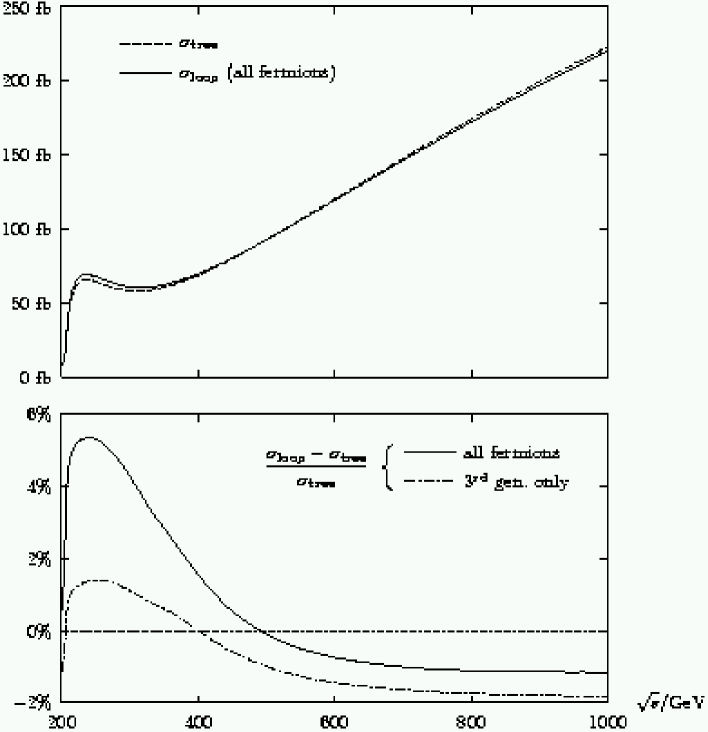
Figure 4.9: The tree-level and the one-loop cross sections for $e^{+}e^{-}\to\bar{\nu}\nu H_{\rm SM}$ in the SM, $\sigma_{H_{\rm SM}}^{0}$ and $\sigma_{H_{\rm SM}}^{1}$, are shown as a function of $\sqrt{s}$ for $M_{H_{\rm SM}}=115\,\,\mathrm{GeV}$. The upper plot shows the absolute values, the lower plot shows the relative corrections for all fermions and for the third-generation fermions only.

Fig. 4.9 shows the tree-level and one-loop-corrected production cross section for a SM Higgs-boson mass of $M_{H_{\rm SM}}=115\,\,\mathrm{GeV}$. The absolute values are shown in the upper plot. The sharp rise in the cross section for $\sqrt{s}\;\raisebox{-3.00003pt}{$\stackrel{{\scriptstyle\displaystyle>}}{{\sim}}$}\;200$ GeV is due to the threshold for on-shell production of the $Z$ boson in the Higgs-strahlung contribution, see the right diagram of Fig. 4.5. Above the threshold the $1/s$ behavior of the Higgs-strahlung contribution competes with the logarithmically rising $t$-channel contribution from $WW$ fusion.

The lower plot shows the relative correction coming from all fermions, as well as the correction from the third-generation fermions only. The correction from all fermions ranges from about $+5\%$ at low $\sqrt{s}$ to $-1.2\%$ at high $\sqrt{s}$. Restricting to the contribution of third-generation fermions only, we obtain corrections in the range from $+1.3\%$ to $-1.8\%$. These corrections (both from the third family only as well as from the first two generations) are at the level of the expected sensitivity for the $WW$-fusion channel at the LC. For a LC running in its high-energy mode with $\sqrt{s}\approx 800$ GeV, in particular, a measurement of the total cross section with an accuracy of better than 2% seems to be feasible [38].

Figure 4.10: The tree-level and the one-loop cross sections for $e^{+}e^{-}\to\bar{\nu}\nu H_{\rm SM}$ in the SM, $\sigma_{H_{\rm SM}}^{0}$ and $\sigma_{H_{\rm SM}}^{1}$, are shown as a function of $M_{H_{\rm SM}}$ for $\sqrt{s}=800,1000\,\,\mathrm{GeV}$.

In Fig. 4.10 the SM production cross section is shown as a function of $M_{H_{\rm SM}}$ for $\sqrt{s}=800,1000\,\,\mathrm{GeV}$. A SM Higgs boson possesses a relatively large production cross section, ${\cal O}(10\,\mbox{fb})$, depending on the available energy, even for $M_{H_{\rm SM}}\;\raisebox{-3.00003pt}{$\stackrel{{\scriptstyle\displaystyle>}}{{\sim}}$}\;500\,\,\mathrm{GeV}$. Thus it should easily be detectable at a high-luminosity LC.

4.2.4 Light ${\cal CP}$-even Higgs-boson production

Since the mass of the lightest ${\cal CP}$-even Higgs boson in the MSSM is bounded from above by $M_{h}\;\raisebox{-3.00003pt}{$\stackrel{{\scriptstyle\displaystyle<}}{{\sim}}$}\;140\,\,\mathrm{GeV}$ [5, 7], its detection at the LC is guaranteed [102]. In order to exploit the precision measurements possible at the LC, a precise prediction at the percent level of its production cross section (and its decay rates) is necessary.

In the following we analyze the $h$ production cross section. To begin with, we focus on the four benchmark scenarios given in the Appendix [53] (proposed for MSSM Higgs-boson searches at hadron colliders and beyond). $M_{A}$ and $\tan\beta$ are kept as free parameters.

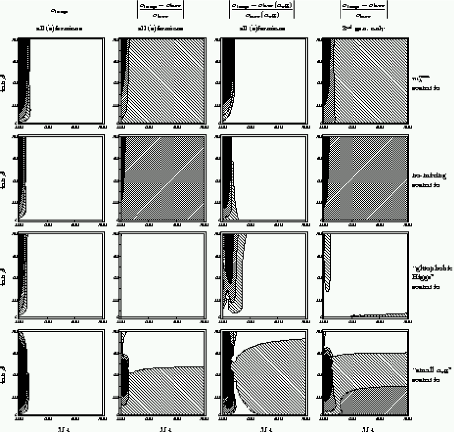
Figure 4.11: Results for the cross section for $e^{+}e^{-}\to\bar{\nu}\nu\,h$ at one-loop order, $\sigma^{1}_{h}$ (left column), the relative corrections including all three fermion and sfermion generations (two middle columns), and the relative corrections including only the third generation (right column) are shown in the $M_{A}$–$\tan\beta$ plane for four benchmark scenarios at $\sqrt{s}=1\,\,\mathrm{TeV}$. The universal Higgs propagator corrections have been absorbed into the tree-level cross section and thus do not appear in the relative corrections. In the second and fourth column the Higgs propagator corrections are implemented according to eqs. (4.40), (4.41), while in the third column the $\alpha_{\rm eff}$ approximation is used. In the results for $\sigma^{1}_{h}$ (left column) the black region corresponds to $\sigma^{1}_{h}<50\,\mbox{fb}$, the dark-shaded region to $50\,\mbox{fb}\leq\sigma^{1}_{h}\leq 100\,\mbox{fb}$, the light-shaded region to $100\,\mbox{fb}\leq\sigma^{1}_{h}\leq 150\,\mbox{fb}$, and the white region to $\sigma^{1}_{h}\geq 150\,\mbox{fb}$. For the relative corrections (second to fourth column) the black region corresponds to $R^{1}_{h}>5\%$, the dark-shaded region to $2\%\leq R^{1}_{h}\leq 5\%$, the light-shaded region to $1\%\leq R^{1}_{h}\leq 2\%$, and the white region corresponds to $R^{1}_{h}\leq 1\%$ (see text).

Figure (4.11) shows in the four benchmark scenarios the $h$ production cross section, $\sigma^{1}_{h}$, eq. (4.42), as well as the relative size of the loop corrections,

$$R^{1}_{h}=\Bigg{|}\frac{\sigma^{1}_{h}-\sigma^{0}_{h}}{\sigma^{0}_{h}}\Bigg{|}$$ (4.45)

(which is nearly always negative), including the contributions from all generations as well as from the third generation only. The results are shown in the $M_{A}$–$\tan\beta$ plane for $100\,\,\mathrm{GeV}\leq M_{A}\leq 400\,\,\mathrm{GeV}$ and $2\leq\tan\beta\leq 50$. For larger $M_{A}$ values the behavior of the lightest ${\cal CP}$-even MSSM Higgs boson is very SM-like, i.e. the results hardly vary with $M_{A}$ any more.

For very low values of $M_{A}$, $M_{A}<150\,\,\mathrm{GeV}$, the cross section is relatively small. This is due to the fact that the $WWh$ coupling at tree level, being $\sim\sin(\beta-\alpha)\hskip 2.84526pt$, can become very small. In this region of parameter space, however, the heavy ${\cal CP}$-even Higgs boson is still very light and couples to the gauge bosons with approximately SM strength, the tree-level coupling of $WWH$ being $\sim\cos(\beta-\alpha)\hskip 2.84526pt\approx 1$.

For the interpretation of the two middle and the right column of Fig. 4.11 it is important to keep in mind that we have absorbed the universal Higgs propagator corrections, which are numerically very important, into our tree-level cross section. Thus, the relative corrections, $R^{1}_{h}$, shown in Fig. 4.11, display the effects of the other genuine one-loop corrections only. We first compare the corrections in the two cases where the Higgs propagator corrections are implemented according to eqs. (4.40), (4.41), which ensures the correct on-shell properties of the outgoing Higgs boson (second column), and where an $\alpha_{\rm eff}$ approximation is used (third column), which is often done in the literature. In the $\alpha_{\rm eff}$ approximation, the leading contribution of the process-independent corrections entering via the Higgs-boson propagators is included by replacing the tree-level coupling of $\{h,H\}WW=\{\sin,\cos\}(\beta-\alpha)$ by $\{\sin,\cos\}(\beta-\alpha_{\rm eff})$. The difference between the full on-shell prescription and the $\alpha_{\rm eff}$ approximation turns out to be sizable. It amounts to several percent even for relatively large values of $M_{A}$. As a consequence, including the Higgs propagator corrections in an $\alpha_{\rm eff}$ approximation will not be sufficient in view of prospective precision measurements of the $e^{+}e^{-}\to\bar{\nu}\nu\,h$ cross section.

The results in the second column of Fig. 4.11 show that the size of the corrections from fermion and sfermion loops is somewhat different in the four scenarios. While corrections of more than 5% only occur for $M_{A}\;\raisebox{-3.00003pt}{$\stackrel{{\scriptstyle\displaystyle<}}{{\sim}}$}\;130\,\,\mathrm{GeV}$, we obtain corrections of 2–5% in the whole parameter space of the no-mixing scenario. Corrections of 1–2% can be found in large parts of the parameter space of the $m_{h}^{\rm max}$ and the small-$\alpha_{\rm eff}$ scenario. The situation in the four benchmark scenarios, which have been chosen to represent different aspects of MSSM phenomenology, shows that the corrections investigated here are typically of the order of about 1–5%. A measurement of the $e^{+}e^{-}\to\bar{\nu}\nu\,h$ cross section at the percent level will thus be sensitive to this kind of corrections.

In the right column of Fig. 4.11 we show $R^{1}_{h}$ derived including the contributions from the third family of fermions and sfermions only. Thus the differences between the second and the fourth column reflect the relevance of the loop corrections coming from the first two families. While in the $m_{h}^{\rm max}$ and the no-mixing scenario differences can mostly be found for small $M_{A}$, $M_{A}\;\raisebox{-3.00003pt}{$\stackrel{{\scriptstyle\displaystyle<}}{{\sim}}$}\;150\,\,\mathrm{GeV}$, in the other two scenarios the effect of the first two families can be relevant also for larger $M_{A}$. Within the gluophobic-Higgs scenario, the first two families play a role for small $\tan\beta$ and large $M_{A}$. In the small-$\alpha_{\rm eff}$ scenario differences can be found for larger $\tan\beta$ over the whole $M_{A}$ range. In the latter two scenarios, the corrections coming from the first and second family lead to a partial compensation of the corrections from the third family. The light fermion generations can give rise to a contribution of $\sim 1\%$, which is non-negligible for cross section measurements at the percent level.

The Higgs propagator corrections, which we have absorbed into our tree-level cross section, mainly affect the numerical value of $M_{h}$, which enters the final-state kinematics, while the numerical effect of the corrections to the $WWh$ coupling is less important. The comparison between the prediction for $e^{+}e^{-}\to\bar{\nu}\nu\,h$ in the MSSM and the corresponding process in the SM for the same value of the Higgs boson mass (which is not shown here) yields deviations of more than 5% for $M_{A}\;\raisebox{-3.00003pt}{$\stackrel{{\scriptstyle\displaystyle<}}{{\sim}}$}\;200\,\,\mathrm{GeV}$, which to a large extent are due to the suppressed $WWh$ coupling in the MSSM case. Deviations of more than 1% are found in all scenarios up to rather large values of $M_{A}$.

Fig. 4.12 shows our results for $e^{+}e^{-}\to\bar{\nu}\nu\,h$ in the four benchmark scenarios as a function of $\sqrt{s}$ for $M_{A}=500\,\,\mathrm{GeV}$ and $\tan\beta=3,40$. Note that the difference in the cross sections for the four benchmark scenarios for given $M_{A}$ and $\tan\beta$ is entirely due to SUSY loop corrections (which, as explained above, affect in particular the value of $M_{h}$).

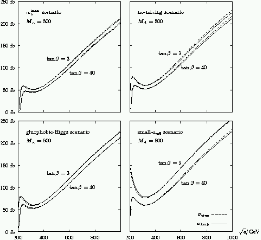
Figure 4.12: The tree-level and the one-loop cross sections for $e^{+}e^{-}\to\bar{\nu}\nu\,h$, $\sigma_{h}^{0}$ and $\sigma_{h}^{1}$, are shown as a function of $\sqrt{s}$ in the four benchmark scenarios for $M_{A}=500\,\,\mathrm{GeV}$ and $\tan\beta=3,40$.

The numerically important effects of the Higgs propagator corrections become apparent in particular from Fig. 4.13, where the tree-level and the one-loop cross sections are shown as a function of $X_{t}$, i.e. the mixing in the scalar top sector. The plots are given for the four combinations of $M_{A}=150,500\,\,\mathrm{GeV}$ and $\tan\beta=3,40$, and the other parameters (besides $X_{t}$) are chosen as in the $m_{h}^{\rm max}$ scenario (see the Appendix). The variation of the tree-level cross sections indicates the effect of the Higgs propagator corrections affecting both the value of $M_{h}$ and the Higgs coupling to gauge bosons. These corrections can change the cross section by up to $\sim 25\%$, while the other loop corrections typically stay below 2.5%.

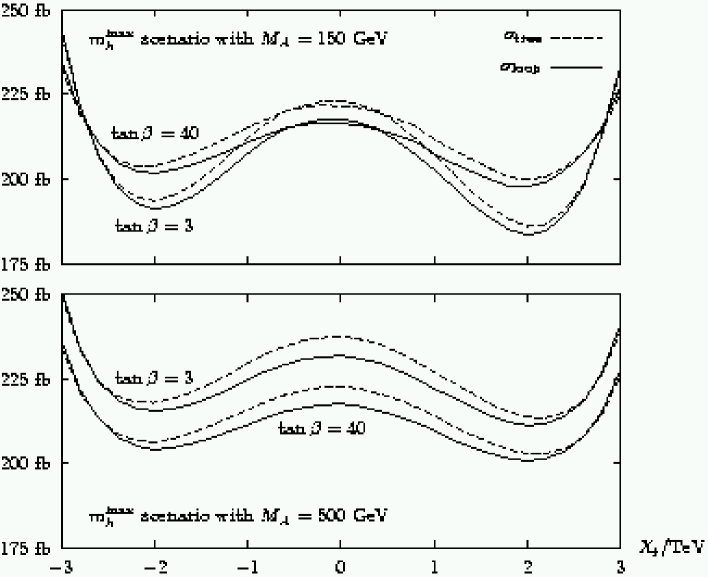
Figure 4.13: The tree-level and the one-loop cross sections for $e^{+}e^{-}\to\bar{\nu}\nu\,h$, $\sigma_{h}^{0}$ and $\sigma_{h}^{1}$, are shown as a function of $X_{t}$. In the upper (lower) plot $M_{A}$ has been set to $M_{A}=150$ $(500)\,\,\mathrm{GeV}$, $\tan\beta$ is fixed at $\tan\beta=3,40$. The other parameters are as given in eq. (2).

Finally, in Fig. 4.14 we analyze the relative importance of the purely sfermionic loop corrections (corresponding to the Feynman diagrams with sfermion loops in Figs. 4.6–4.8; as before, the Higgs propagator corrections absorbed into the tree-level result contain both fermion- and sfermion-loop contributions). These corrections constitute, as explained earlier, a UV-finite and gauge-invariant subset of the loop contributions. The relative size of the sfermion corrections as compared to the purely fermionic one-loop corrections is shown in Fig. 4.14. The upper row shows the relative size as a function of $X_{t}$ in the $m_{h}^{\rm max}$ scenario for all combinations of $M_{A}=150,500\,\,\mathrm{GeV}$ and $\tan\beta=3,40$. While for $X_{t}\approx 0$, i.e. for small splitting in the scalar top sector, the sfermionic corrections are small, their contribution becomes more important for increasing $|X_{t}|$. They have the opposite sign of the purely fermionic corrections and thus partially compensate their effects. For $|X_{t}/M_{\rm SUSY}|\approx 2$ the sfermionic corrections are about half as large as the fermion corrections. For very large $|X_{t}|$ (which also lowers $M_{h}$ substantially) they can become even bigger than the fermionic ones.

In the lower part of Fig. 4.14 (middle and lower row) we analyze the relative size of the purely sfermionic corrections in the $m_{h}^{\rm max}$ (middle) and the no-mixing scenario (lower row) as a function of $M_{\rm SUSY}$. In the no-mixing scenario, for increasing $M_{\rm SUSY}$ the relative size of the sfermion corrections becomes smaller, as can be expected in the decoupling limit [103, 104]. In the $m_{h}^{\rm max}$ scenario, however, the situation is different. Here $X_{t}\approx A_{t}$ is fixed to $A_{t}\approx X_{t}=2\,M_{\rm SUSY}$. In the $h\tilde{t}_{1}\tilde{t}_{2}$ vertex, being $\sim A_{t}\cos\alpha\hskip 2.84526pt+\mu\sin\alpha\hskip 2.84526pt$, the coupling is proportional to the SUSY mass scale. This results in a term $\sim A_{t}/M_{\rm SUSY}$ in the one-loop corrected $WWh$ vertex, which for large $M_{\rm SUSY}$ goes to a constant and can be of the order of the purely fermionic correction. The cross section then behaves as $\sim X_{t}^{2}/M_{\rm SUSY}^{2}$ as can be seen in the upper row of Fig. 4.14.

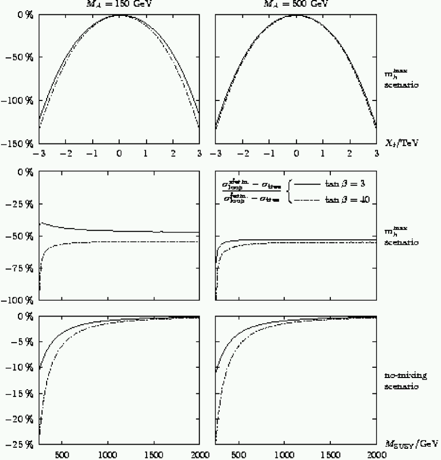
Figure 4.14: The relative size of the purely sfermionic loop corrections to $\sigma^{1}_{h}$ as compared to the purely fermionic one-loop corrections is shown as a function of $X_{t}$ (upper) and $M_{\rm SUSY}$ (middle and lower row) for all combinations of $M_{A}=150,500\,\,\mathrm{GeV}$ and $\tan\beta=3,40$. The other parameters are chosen as in the $m_{h}^{\rm max}$ (upper and middle) or as in the no-mixing scenario (lower row).

4.2.5 Heavy ${\cal CP}$-even Higgs-boson production

We now investigate the effects of loop corrections on the cross section for heavy ${\cal CP}$-even Higgs-boson production in the MSSM. As explained above, these corrections are of particular interest in the decoupling region, i.e. for large values of $M_{A}$. If $M_{A}\;\raisebox{-3.00003pt}{$\stackrel{{\scriptstyle\displaystyle<}}{{\sim}}$}\;\sqrt{s}/2$, the heavy Higgs bosons can be pair-produced at the LC via $e^{+}e^{-}\to Z^{*}\to HA$. Beyond this kinematical limit, $H$ production is in principle possible via the $WW$-fusion and the Higgs-strahlung channels. This production mechanism is heavily suppressed at tree-level, however, owing to the decoupling property of the $H$ coupling to gauge bosons. If loop-induced contributions turn out to be sizable in the mass range $M_{H}>\sqrt{s}/2$, an enhanced reach of the LC for $H$ production could result.

               

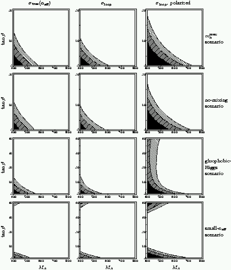
Figure 4.15: The tree-level cross section for $e^{+}e^{-}\to\bar{\nu}\nu\,H$, $\sigma^{0}_{H}(\alpha_{\rm eff})$, using an $\alpha_{\rm eff}$ approximation (left), and the one-loop cross sections, $\sigma^{1}_{H}$, without (middle), and with beam polarization (right column), are shown in the $M_{A}$–$\tan\beta$ plane for four benchmark scenarios for $\sqrt{s}=1\,\,\mathrm{TeV}$. The different shadings correspond to: white: $\sigma\leq 0.01\,\mbox{fb}$, light shaded: $0.01\,\mbox{fb}\leq\sigma\leq 0.02\,\mbox{fb}$, dark shaded: $0.02\,\mbox{fb}\leq\sigma\leq 0.05\,\mbox{fb}$, black: $\sigma\geq 0.05\,\mbox{fb}$.

In Fig. 4.15 we first compare the tree-level cross section evaluated in the $\alpha_{\rm eff}$ approximation, $\sigma_{H}^{0}(\alpha_{\rm eff})$ (left column), and the one-loop cross section according to eq. (4.44), $\sigma_{H}^{1}$ (middle column), in the four benchmark scenarios. For phenomenological analyses of MSSM Higgs-boson production in this channel the cross section has so far mostly been evaluated using an $\alpha_{\rm eff}$ Born approximation (see also Sect. 4.2.4).

We concentrate on the case of $\sqrt{s}=1\,\,\mathrm{TeV}$. Since we are interested in $M_{H}\approx M_{A}>\sqrt{s}/2=500\,\,\mathrm{GeV}$, we focus on the region $400\,\,\mathrm{GeV}\leq M_{A}\leq 900\,\,\mathrm{GeV}$, and scan over the whole $\tan\beta$ region. For a LC like TESLA, the anticipated integrated luminosity is of ${\cal O}(2\mbox{ab}^{-1})$. For this luminosity, a production cross section of about $\sigma_{H}=0.01\,\mbox{fb}$ constitutes a lower limit for the observation of the heavy ${\cal CP}$-even Higgs boson. (For the scenarios discussed below, the dominant decay channel of $H$ is the decay into $t\bar{t}$ or $b\bar{b}$, depending on the value of $\tan\beta$, and also sizable branching ratios into SUSY particles are possible in some regions of parameter space; a more detailed simulation of this process should of course take into account the impact of the decay characteristics on the lower limit of observability, while in this work we use the approximation of a universal limit.) The area with $\sigma_{H}\leq 0.01\,\mbox{fb}$ is shown in white in Fig. 4.15. In the four benchmark scenarios shown in Fig. 4.15, the inclusion of the loop corrections that go beyond the $\alpha_{\rm eff}$ Born approximation turns out to have only a moderate effect on the area in the $M_{A}$–$\tan\beta$ plane in which $H$ production could be observable. While for the $m_{h}^{\rm max}$ and the no-mixing scenario the area is slightly decreased to smaller $\tan\beta$ values and somewhat enlarged to higher $M_{A}$ values, the area is slightly decreased in $\tan\beta$ in the gluophobic-Higgs scenario (and stays approximately the same in $M_{A}$), while the area is slightly enlarged both in $M_{A}$ and $\tan\beta$ in the small-$\alpha_{\rm eff}$ scenario. For the four benchmark scenarios, an observation with $M_{H}>500\,\,\mathrm{GeV}$ is only possible for low $\tan\beta$, $\tan\beta\;\raisebox{-3.00003pt}{$\stackrel{{\scriptstyle\displaystyle<}}{{\sim}}$}\;5$, where the LC reach in $M_{H}$ can be extended by up to $100\,\,\mathrm{GeV}$. It should be noted at this point that while the area of observability is modified only slightly in the plots as a consequence of including the loop corrections, the relative changes between the tree-level and the one-loop values of the cross sections can be very large, owing to the suppressed $WWH$ coupling in the tree-level cross section.

The prospects for observing a heavy Higgs boson beyond the kinematical limit of the $HA$ pair production channel become more favorable, however, if polarized beams are used. The cross section becomes enhanced for left-handedly polarized electrons and right-handedly polarized positrons. While a 100% polarization results in a cross section that is enhanced roughly by a factor of 4, more realistic values of 80% polarization for electrons and 60% polarization for positrons [105] would yield roughly an enhancement by a factor of 3. The right column of Fig. 4.15 shows the four benchmark scenarios with 100% polarization of both beams. The area in the $M_{A}$–$\tan\beta$ plane in which observation of the $H$ boson might become possible is strongly increased in this case. In the $m_{h}^{\rm max}$ and the no-mixing scenario, $H$ observation could be possible for small $\tan\beta$ up to $M_{A}\;\raisebox{-3.00003pt}{$\stackrel{{\scriptstyle\displaystyle<}}{{\sim}}$}\;700\,\,\mathrm{GeV}$. In the gluophobic-Higgs and the small-$\alpha_{\rm eff}$ scenario this effect is somewhat smaller. In the latter scenario the discovery of a heavy Higgs boson in the parameter region $M_{A}>500\,\,\mathrm{GeV}$ will become possible also for large $\tan\beta$, $\tan\beta\;\raisebox{-3.00003pt}{$\stackrel{{\scriptstyle\displaystyle>}}{{\sim}}$}\;35$.

While without the inclusion of beam polarization we do not find a significant enhancement of the LC discovery reach as a consequence of the loop corrections in the four benchmark scenarios analyzed in Fig. 4.15, this behavior changes in other regions of the MSSM parameter space. As a particular example, we investigate the $M_{A}$–$\tan\beta$ plane in the “$\sigma_{H}^{\text{enh}}$” (“enhanced cross section”) scenario, which is defined by

$$M_{\rm SUSY}=350\,\,\mathrm{GeV},\quad\mu=1000\,\,\mathrm{GeV},$$ (4.46)

with the other parameters as in the $m_{h}^{\rm max}$ scenario, eq. (2). The $\sigma_{H}^{\text{enh}}$ scenario is thus characterized by a relatively small value of $M_{\rm SUSY}$ and a relatively large value of $\mu$. Large $\tan\beta$ values, $\tan\beta\;\raisebox{-3.00003pt}{$\stackrel{{\scriptstyle\displaystyle>}}{{\sim}}$}\;30$, can result in low and experimentally ruled-out $\tilde{b}$ masses and are therefore omitted.

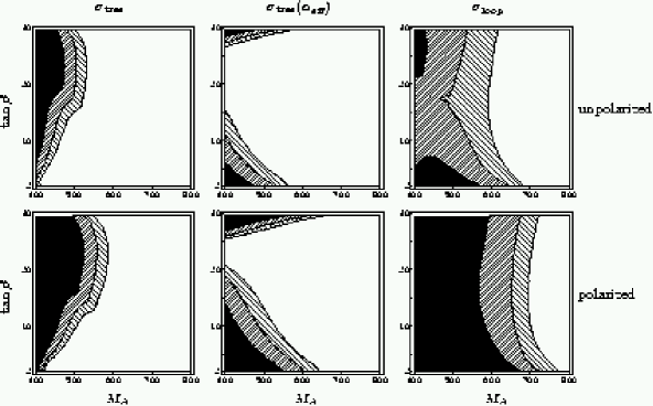
Figure 4.16: The cross sections for $e^{+}e^{-}\to\bar{\nu}\nu\,H$ are shown in the $M_{A}$–$\tan\beta$ plane for the $\sigma_{H}^{\text{enh}}$ scenario, eq. (4.46). The tree-level cross section (left) including the finite wave-function corrections is compared to the $\alpha_{\rm eff}$ approximation (middle) and the one-loop corrected cross section (right column). The upper (lower) row shows the production cross section for unpolarized (100% polarized) electron and positron beams. The color coding is as in Fig. 4.15.

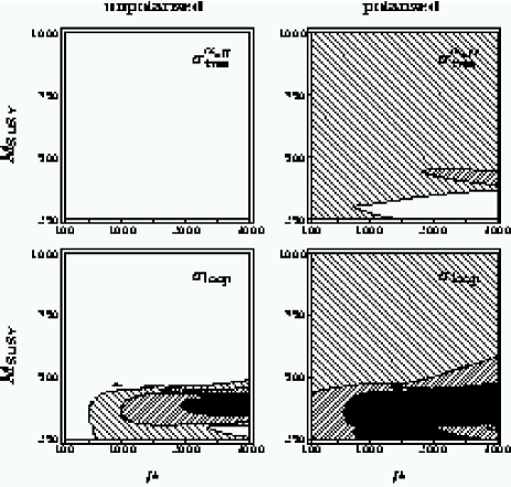
Figure 4.17: The tree-level cross section for $e^{+}e^{-}\to\bar{\nu}\nu\,H$, $\sigma^{0}_{H}(\alpha_{\rm eff})$, using an $\alpha_{\rm eff}$ approximation (upper), and the one-loop cross section, $\sigma^{1}_{H}$ (lower row), are shown in the $\mu$–$M_{\rm SUSY}$ plane for the parameters of eq. (2) and $M_{A}=600\,\,\mathrm{GeV}$ and $\tan\beta=4$. The left column shows the unpolarized case, while in the right column the effects of beam polarization are included. The color coding is as in Fig. 4.15.

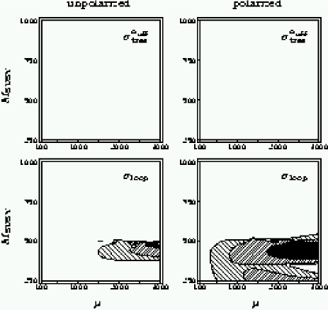
Figure 4.18: The tree-level cross section for $e^{+}e^{-}\to\bar{\nu}\nu\,H$, $\sigma^{0}_{H}(\alpha_{\rm eff})$, using an $\alpha_{\rm eff}$ approximation (upper), and the one-loop cross section, $\sigma^{1}_{H}$ (lower row), is shown in the $\mu$–$M_{\rm SUSY}$ plane for the parameters of eq. (2) and $M_{A}=700\,\,\mathrm{GeV}$ and $\tan\beta=4$. The left column shows the unpolarized case, while in the right column the effects of beam polarization are included. The color coding is as in Fig. 4.15.

In the upper row of Fig. 4.16 we compare $\sigma_{H}^{0}$, $\sigma_{H}^{0}(\alpha_{\rm eff})$, and $\sigma_{H}^{1}$ for the parameters of the $\sigma_{H}^{\text{enh}}$ scenario, eq. (4.46), in the unpolarized case. The figure shows that both the inclusion of the finite Higgs propagator wave-function corrections, see eqs. (4.32)-(4.33), as compared to the $\alpha_{\rm eff}$ approximation (left vs. middle column) and of the genuine one-loop corrections (right vs. left column) is very important in this scenario. According to the $\alpha_{\rm eff}$ Born approximation, the parameter area in which observation of $H$ is possible would not be significantly larger than in the benchmark scenarios discussed in Fig. 4.15. For $M_{A}\;\raisebox{-3.00003pt}{$\stackrel{{\scriptstyle\displaystyle>}}{{\sim}}$}\;500\,\,\mathrm{GeV}$, observation of the $H$ boson is only possible for either rather small, $\tan\beta\;\raisebox{-3.00003pt}{$\stackrel{{\scriptstyle\displaystyle<}}{{\sim}}$}\;5$, or rather large, $\tan\beta\;\raisebox{-3.00003pt}{$\stackrel{{\scriptstyle\displaystyle>}}{{\sim}}$}\;28$, values of $\tan\beta$. Inclusion of the finite Higgs propagator wave-function corrections, which ensure the correct on-shell properties of the outgoing Higgs boson, changes the situation considerably. While for small and large values of $\tan\beta$ the additional corrections suppress the $e^{+}e^{-}\to\bar{\nu}\nu\,H$ cross section, restricting the $H$ observability to values of $M_{A}$ below 500 GeV, observation of the heavy ${\cal CP}$-even Higgs boson of the MSSM becomes possible for $M_{A}\;\raisebox{-3.00003pt}{$\stackrel{{\scriptstyle\displaystyle<}}{{\sim}}$}\;550\,\,\mathrm{GeV}$ for a significant range of intermediate values of $\tan\beta$. Including also the genuine one-loop corrections (right column) leads to a further drastic enhancement of the parameter space in which the $H$ boson could be observed. The observation of the $H$ boson will be possible in this scenario for all values of $\tan\beta$ if $M_{A}\;\raisebox{-3.00003pt}{$\stackrel{{\scriptstyle\displaystyle<}}{{\sim}}$}\;600\,\,\mathrm{GeV}$, i.e. the discovery reach of the LC in this case is enhanced by about 100 GeV compared to the $HA$ pair production channel.

The prospects in this scenario for observation of the heavy ${\cal CP}$-even Higgs boson of the MSSM become even more favorable if polarized beams are used. The lower row of Fig. 4.16 shows the situation with 100% polarization of both beams for the $\sigma_{H}^{\text{enh}}$ scenario, eq. (4.46). While in this case the tree-level result (both for the case including the finite wave-function corrections and for the $\alpha_{\rm eff}$ approximation) gives rise to observable rates for $M_{A}\;\raisebox{-3.00003pt}{$\stackrel{{\scriptstyle\displaystyle<}}{{\sim}}$}\;600\,\,\mathrm{GeV}$ for a certain range of $\tan\beta$ values only, the further genuine loop corrections enhance the cross section significantly. In this situation the observation of the heavy ${\cal CP}$-even Higgs boson might be possible for values of $M_{A}$ up to about 700–750 GeV for all $\tan\beta$ values, corresponding to an enhancement of the LC reach by more than $200\,\,\mathrm{GeV}$. Cross-section values in excess of $0.05\,\mbox{fb}$ are obtained in this example for all $\tan\beta$ values for $M_{A}\;\raisebox{-3.00003pt}{$\stackrel{{\scriptstyle\displaystyle<}}{{\sim}}$}\;600\,\,\mathrm{GeV}$.

In order to investigate whether this result is a consequence of a very special choice of SUSY parameters or a more general feature, in Fig. 4.17 we choose the parameters of the $m_{h}^{\rm max}$ scenario for a fixed combination of $M_{A}$ and $\tan\beta$, $M_{A}=600\,\,\mathrm{GeV}$, $\tan\beta=4$, but scan over $\mu$ and $M_{\rm SUSY}$. The choice $M_{H}\approx M_{A}=600\,\,\mathrm{GeV}$ implies that the $HA$ production channel is clearly beyond the reach of a 1 TeV LC. The upper row of Fig. 4.17 shows that according to the tree-level cross section (using the $\alpha_{\rm eff}$ approximation) an observable rate for a heavy ${\cal CP}$-even Higgs boson with $M_{A}=600\,\,\mathrm{GeV}$ cannot be found for any of the scanned values of $\mu$ and $M_{\rm SUSY}$. Inclusion of the further loop corrections changes this situation significantly and gives rise to observable rates in this example for nearly all $M_{\rm SUSY}\;\raisebox{-3.00003pt}{$\stackrel{{\scriptstyle\displaystyle<}}{{\sim}}$}\;500\,\,\mathrm{GeV}$ if $\mu\;\raisebox{-3.00003pt}{$\stackrel{{\scriptstyle\displaystyle>}}{{\sim}}$}\;500\,\,\mathrm{GeV}$. The visible “structure” at $M_{\rm SUSY}\approx 500\,\,\mathrm{GeV}$ is the result of several competing effects that affect the finite Higgs wave-function corrections.

The same analysis, but with 100% polarization of both beams, is shown in the right column of Fig. 4.17. The tree-level $\alpha_{\rm eff}$ approximation results in an observable rate in nearly the whole plane apart from the area with $\mu\;\raisebox{-3.00003pt}{$\stackrel{{\scriptstyle\displaystyle>}}{{\sim}}$}\;1000\,\,\mathrm{GeV}$ and $M_{\rm SUSY}\;\raisebox{-3.00003pt}{$\stackrel{{\scriptstyle\displaystyle<}}{{\sim}}$}\;350\,\,\mathrm{GeV}$. Adding the loop corrections again improves the situation. No unobservable holes remain in the $\mu$–$M_{\rm SUSY}$ plane, i.e. the heavy ${\cal CP}$-even Higgs boson with $M_{H}\approx 600\,\,\mathrm{GeV}$ should be visible at a 1 TeV LC with (idealized) beam polarization in this scenario. The production cross section is larger than $0.02\,\mbox{fb}$ for all $\mu$ and $M_{\rm SUSY}\;\raisebox{-3.00003pt}{$\stackrel{{\scriptstyle\displaystyle<}}{{\sim}}$}\;500\,\,\mathrm{GeV}$ and mostly even larger than $0.05\,\mbox{fb}$ for $\mu\;\raisebox{-3.00003pt}{$\stackrel{{\scriptstyle\displaystyle>}}{{\sim}}$}\;500\,\,\mathrm{GeV}$.

The same analysis, but for an even larger Higgs boson mass scale, $M_{A}=700\,\,\mathrm{GeV}$ is shown in Fig. 4.18. For the $\alpha_{\rm eff}$ approximation the production cross section is lower than $0.01\,\mbox{fb}$ in the whole $\mu$–$M_{\rm SUSY}$-plane. However, for the loop corrected cross section, especially including polarization, the heavy ${\cal CP}$-even Higgs boson could be observable for all $\mu$ values for $M_{\rm SUSY}\;\raisebox{-3.00003pt}{$\stackrel{{\scriptstyle\displaystyle<}}{{\sim}}$}\;500\,\,\mathrm{GeV}$.

         

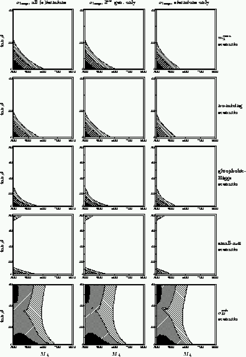
Figure 4.19: $\sigma_{H}^{1}$ is shown in the $M_{A}$–$\tan\beta$ plane for the four benchmark scenarios defined in eqs. (2)–(5) and the $\sigma_{H}^{\text{enh}}$ scenario for $\sqrt{s}=1\,\,\mathrm{TeV}$ in the unpolarized case. The one-loop result containing the corrections from all fermion and sfermion loops (left) is compared with the result from only third-generation fermions and sfermions (middle) and the purely sfermionic corrections from all families (right column). The color coding is as in Fig. 4.15.

In Fig. 4.19 we compare for all five scenarios analyzed in this section the results for the cross section when different parts of the generic one-loop corrections are taken into account. In all cases the full result for the Higgs propagator corrections being absorbed in the lowest-order cross section are employed. The left column shows the result containing the corrections from all fermion and sfermion loops, $\sigma_{H}^{1}$, which is repeated from previous plots for comparison purposes. The middle column shows the cross-section prediction based on taking into account only the corrections from the third-generation fermions and sfermions, which have turned out to be the leading corrections for the light Higgs-boson production. The result shown in the right column have been obtained by including only the purely sfermionic contributions from all generations, i.e. the fermion-loop corrections are omitted in this case. As expected from Fig. 4.15, in the four scenarios defined in the Appendix, where the loop corrections turned out to modify the parameter regions in which $H$ observation becomes possible only slightly, omitting the contributions of the first two generations of fermions and sfermions and of the fermion loops of all three generations does not lead to a qualitative change in the $H$ discovery reach. In the $\sigma_{H}^{\text{enh}}$ scenario, on the other hand, the genuine one-loop corrections had a considerable impact on the area in the $M_{A}$–$\tan\beta$ plane in which $H$ observation is possible, see Fig. 4.16. The result displayed in the middle column for this scenario shows that the bulk of the corrections comes from the third generation of fermions and sfermions, i.e. omission of the first two generations does not lead to significant effects in the $M_{A}$–$\tan\beta$ plane. The result in the right column for this scenario shows furthermore that the omission of all fermion-loop corrections leads only to very moderate changes of the parameter regions where $H$ observation is possible. As a consequence, the by far dominant corrections in this scenario can be identified as the ones from the sfermions of the third generation. This is contrary to the $h$ production, where we found that the fermionic corrections are mostly larger than the sfermionic ones.

4.3 Single charged Higgs boson production

In this section the dominant contributions to the process $e^{+}e^{-}\to e\nu_{e}\,H^{\pm}$ [95] are briefly described. Since there is no $\{\gamma,Z\}W^{\pm}H^{\mp}$ coupling, the single charged-Higgs production starts at the one-loop level. As for $e^{+}e^{-}\to\nu\bar{\nu}\{h,H\}$, we take into account the leading corrections arising from the full set of SM fermion and sfermion loops. Bremsstrahlung diagrams are suppressed by an additional ${\cal O}(\alpha)$ as compared to the leading contribution and have thus been omitted.

4.3.1 Calculation

The loop corrections that enter the process $e^{+}e^{-}\to e\nu_{e}\,H^{\pm}$ at the one-loop level are generically depicted in Figs. 4.20, 4.21. The contributions involve all corrections from fermion and sfermion loops (which give contributions only to self-energies and vertices). Contributions $\propto m_{e}/M_{W}$ were neglected.

Figure 4.20: Generic self-energy diagrams for the process $e^{+}e^{-}\to e\nu_{e}\,H^{\pm}$.

Figure 4.21: Generic vertex diagrams for the process $e^{+}e^{-}\to e\nu_{e}\,H^{\pm}$.

Furthermore, counterterm contributions are needed for the $W^{\pm}H^{\mp}$ self-energy corrections, see Ref. [94]. In order to generate the counterterms it is sufficient to introduce the field renormalization for the $H^{\pm}-W^{\pm}$ mixing, $\delta Z_{HW}$. This yields the Feynman rules:

$$\Gamma_{\text{CT}}[H^{\mp}W^{\pm}(k^{\mu})] =i\frac{k^{\mu}}{M_{W}}M_{W}^{2}\,\delta Z_{HW}\;,$$ (4.47)

$$\Gamma_{\text{CT}}[\gamma_{\mu}W^{\pm}_{\nu}H^{\mp}] =-ieM_{W}g_{\mu\nu}\,\delta Z_{HW}\;,$$ (4.48)

$$\Gamma_{\text{CT}}[Z_{\mu}W^{\pm}_{\nu}H^{\mp}] =ieM_{W}\frac{s_{w}}{c_{w}}g_{\mu\nu}\,\delta Z_{HW}$$ (4.49)

In the on-shell scheme $\delta Z_{HW}$ is given by

$$\delta Z_{HW} =\frac{1}{M_{W}^{2}}\,\mbox{Re}\,\Sigma_{HW}(M_{H^{\pm}}^{2})~{}.$$ (4.50)

4.3.2 Results

The results for $H^{+}$ and $H^{-}$ production are the same if CP is not violated (which we assume in this section). In Fig. 4.22 we show the typical size of the production cross section for $e^{+}e^{-}\to e^{+}\nu_{e}\,H^{-}$ for unpolarized external particles. The parameters are chosen according to the four benchmark scenarios described in the Appendix, with $M_{A}=250\,\,\mathrm{GeV}$ and $\tan\beta=2$ and $10$ (with $M_{H^{\pm}}\approx 262\,\,\mathrm{GeV}$). Concerning the discovery of the charged Higgs boson, the cross section has to be doubled, due to the production of both, $H^{+}$ and $H^{-}$.

In Fig. 4.22 the cross section for $e^{+}e^{-}\to e^{+}\nu_{e}\,H^{-}$ is shown as a function of $\sqrt{s}$. The rise of the cross section at $\sqrt{s}\approx M_{H^{\pm}}+M_{W}$ is due to the $W$ propagator in the type of diagram on the right becoming resonant. The resonance was treated with a fixed $W$ width. No cut on the electron emission angle had to be put, since the result is finite in the limit of forward electron scattering.

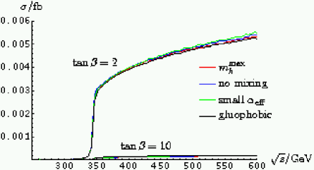
Figure 4.22: The $e^{+}e^{-}\to e^{+}\nu_{e}\,H^{-}$ production cross section as a function of $\sqrt{s}$.

The variation within the four benchmark scenarios is small. For $\tan\beta=10$ the charged-Higgs production cross section stays at a negligible level. Even for $\tan\beta=2$ it stays below $0.01\,\mbox{fb}$ for $2\,M_{H^{\pm}}\approx\sqrt{s}\lesssim 500\,\,\mathrm{GeV}$. Using polarized $e^{+}$ and $e^{-}$ beams, the cross section could be enhanced by about a factor of 2. In summary, however, the single charged-Higgs production, $e^{+}e^{-}\to e\nu_{e}\,H^{\pm}$, could increase the potential of a LC for the detection of the heavy MSSM Higgs-boson spectrum only for parameters beyond the typical benchmark scenarios.

Chapter 5 Higgs boson decays to SM fermions

After the detection of a scalar particle it is mandatory as a next step to measure its couplings to gauge bosons and fermions and also its self-couplings very accurately, in order to establish the Higgs mechanism and the Yukawa interactions experimentally. The determination of the trilinear Higgs-boson self-couplings might be possible at a future linear $e^{+}e^{-}$ collider with high luminosity [41].

In this section we concentrate on the Feynman-diagrammatic corrections (i.e. beyond the effective coupling approximation) to the coupling of the lightest MSSM Higgs boson to SM fermions. Since the $b$-, the $c$-quark and the $\tau$-lepton are the heaviest particles for which the decay $h\to f\bar{f}$ is kinematically allowed, it is of particular interest to calculate the corresponding decay rates and branching ratios with high precision [11, 106, 107, 108, 82, 109, 110, 99]. We analyze these decay rates and branching ratios, taking into account the Higgs-boson propagator corrections, where at the one-loop level the full momentum dependence is kept [99]. We also take into account the one-loop vertex corrections resulting from gluon, gluino, and photon exchange together with real gluon and photon emission as given in Ref. [11]. Only the purely weak ${\cal O}(\alpha)$ vertex corrections have been neglected (see e.g. Ref. [111] for a recent evaluation). We numerically investigate the effect of the two-loop propagator contributions and the one-loop gluino-exchange vertex correction. The latter is supplemented with a resummation of the leading contributions of ${\cal O}((\alpha_{s}\tan\beta)^{n})$, see Sect. 2.3.4. Some phenomenological consequences are investigated.

We show analytically that the Higgs-boson propagator correction with neglected momentum dependence can be absorbed into the tree-level coupling using the effective mixing angle from the neutral ${\cal CP}$-even Higgs boson sector [99]. The result in this approximation is then compared with the full result.

5.1 Higher-order corrections to $h\to f\bar{f}$

5.1.1 Calculation of the decay amplitude

Our main emphasis in this section is on the fermionic decays of the light Higgs boson, but for completeness we list the expressions for both $h$ and $H$. The amplitudes for the decays $h,H\to f\bar{f}$ can be written as follows:

$$A(h\to f\bar{f}) = \sqrt{\hat{Z}_{h}}\left(\Gamma_{h}+\hat{Z}_{hH}\;\Gamma_{H}\right)~{},$$ (5.1)

$$A(H\to f\bar{f}) = \sqrt{\hat{Z}_{H}}\left(\Gamma_{H}+\hat{Z}_{Hh}\;\Gamma_{h}\right)~{},$$ (5.2)

with $\hat{Z}_{h},\hat{Z}_{H},\hat{Z}_{hH}$ and $\hat{Z}_{Hh}$ given in eqs. (4.34)-(4.37).

5.1.2 The $\alpha_{\rm eff}$ approximation for decay amplitudes

The dominant contributions for the Higgs boson self-energies can be obtained by setting $q^{2}=0$, see Sect. 2.3.3:

$$\hat{\Sigma}(q^{2})\to\hat{\Sigma}(0)\equiv\hat{\Sigma}~{}.$$ (5.3)

With the approximation (5.3) (see also eqs. (2.92), (2.93)) one deduces

$$\hat{Z}_{hH} = -\frac{\hat{\Sigma}_{hH}}{M_{h}^{2}-m_{H}^{2}+\hat{\Sigma}_{HH}}=-\tan\Delta\alpha,$$ (5.4)

$$\hat{Z}_{Hh} = -\frac{\hat{\Sigma}_{hH}}{M_{H}^{2}-m_{h}^{2}+\hat{\Sigma}_{hh}}=+\tan\Delta\alpha,$$ (5.5)

and $Z_{h}$ can be expressed as

$$\hat{Z}_{h} = \frac{1}{1+\left(\frac{\hat{\Sigma}_{hH}}{M_{h}^{2}-m_{H}^{2}+\hat{\Sigma}_{HH}}\right)^{2}}$$ (5.6)

$$= \frac{1}{1+\tan^{2}\Delta\alpha}=\cos^{2}\Delta\alpha~{}.$$

Analogously one obtains

$$\hat{Z}_{H}=\cos^{2}\Delta\alpha~{}.$$ (5.7)

At tree level, the vertex functions can be written as

$$\left.\begin{array}[]{l}\Gamma_{h}=\frac{iem_{f}\sin\alpha\hskip 2.84526pt}{2s_{\mathrm{w}}M_{W}\cos\beta\hskip 2.84526pt}=C_{f}^{(d)}\;\sin\alpha\\ \Gamma_{H}=\frac{-iem_{f}\cos\alpha\hskip 2.84526pt}{2s_{\mathrm{w}}M_{W}\cos\beta\hskip 2.84526pt}=-C_{f}^{(d)}\;\cos\alpha\end{array}\right\}\mbox{for d-type fermions},$$ (5.10)

$$\left.\begin{array}[]{l}\Gamma_{h}=\frac{-iem_{f}\cos\alpha\hskip 2.84526pt}{2s_{\mathrm{w}}M_{W}\sin\beta}=C_{f}^{(u)}\;\cos\alpha\\ \Gamma_{H}=\frac{-iem_{f}\sin\alpha\hskip 2.84526pt}{2s_{\mathrm{w}}M_{W}\sin\beta}=C_{f}^{(u)}\;\sin\alpha\end{array}\right\}\mbox{for u-type fermions}~{}.$$ (5.13)

Incorporating them into the decay amplitude yields the corresponding $\alpha_{\rm eff}$ approximation:

$$A_{\rm eff}(h\to f\bar{f}) = \sqrt{Z_{h}}\left(\Gamma_{h}+Z_{hH}\;\Gamma_{H}\right)$$ (5.14)

$$= C_{f}^{(d)}\cos\Delta\alpha\left(\sin\alpha\hskip 2.84526pt-\tan\Delta\alpha\left(-\cos\alpha\hskip 2.84526pt\right)\right)$$

$$= C_{f}^{(d)}\sin(\alpha+\Delta\alpha)$$

$$\equiv C_{f}^{(d)}\sin\alpha_{\rm eff}~{}~{}~{}\mbox{(for d-type fermions)},$$

$$A_{\rm eff}(h\to f\bar{f}) \equiv C_{f}^{(u)}\cos\alpha_{\rm eff}~{}~{}~{}\mbox{(for u-type fermions)},$$ (5.15)

$$A_{\rm eff}(H\to f\bar{f}) \equiv -C_{f}^{(d)}\cos\alpha_{\rm eff}~{}~{}~{}\mbox{(for d-type fermions)},$$ (5.16)

$$A_{\rm eff}(H\to f\bar{f}) \equiv C_{f}^{(u)}\sin\alpha_{\rm eff}~{}~{}~{}\mbox{(for u-type fermions)}~{}.$$ (5.17)

5.1.3 Evaluation of the Higgs-boson propagator corrections

The Higgs boson self-energies employed in the field renormalization constants, see eqs. (4.34)–(4.37), have been evaluated in the Feynman-diagrammatic approach according to

$$\hat{\Sigma}_{s}(q^{2})=\hat{\Sigma}^{(1)}_{s}(q^{2})+\hat{\Sigma}^{(2)}_{s}(0)~{},~{}~{}s=h,H,hH~{},$$ (5.18)

where the momentum dependence has been neglected only at the two-loop level, while the full momentum dependence is kept in the one-loop contributions, see Sect. 2.3.4.

For the numerical evaluation in a first step of approximation for the calculation of the decay width $\Gamma(h\to f\bar{f})$ the momentum dependence is neglected everywhere in the Higgs boson self-energies, the $q^{2}=0$ approximation (see eq. (5.3)):

$$\hat{\Sigma}_{s}(q^{2})\to\hat{\Sigma}^{(1)}_{s}(0)+\hat{\Sigma}^{(2)}_{s}(0)~{},~{}~{}s=h,H,hH~{}.$$ (5.19)

This corresponds to the $\alpha_{\rm eff}$-approximation, as described in Sect. 5.1.2.

In a second step of approximation we approximate the Higgs boson self-energies by the compact analytical formulas given in Ref. [17]:

$$\hat{\Sigma}_{s}(q^{2})=\hat{\Sigma}_{s}^{(1)\rm\,approx}(0)+\hat{\Sigma}_{s}^{(2)\rm\,approx}(0)~{},~{}~{}s=h,H,hH~{}.$$ (5.20)

Here the full result of the self-energy corrections is approximated by an expansion in terms of $m_{t}/M_{\rm SUSY}$ and $X_{t}/M_{\rm SUSY}$, yielding relatively short expressions which allow a very fast numerical evaluation. In the following, this approximation is labeled by $\alpha_{\rm eff}{\rm(approx)}$.

5.1.4 Decay width of the lightest Higgs boson

At the tree level, the decay width for $h\to f\bar{f}$ is given by

$$\Gamma_{0}(h\to f\bar{f})=N_{C}\frac{m_{h}}{8\,\pi}\left(1-\frac{4\,m_{f}^{2}}{m_{h}^{2}}\right)^{\frac{3}{2}}~{}|\Gamma_{h}|^{2}~{}.$$ (5.21)

The electroweak propagator corrections are incorporated by using the higher-order decay amplitude (5.1)

$$\Gamma_{1}\equiv\Gamma_{1}(h\to f\bar{f})=N_{C}\frac{M_{h}}{8\,\pi}\left(1-\frac{4\,m_{f}^{2}}{M_{h}^{2}}\right)^{\frac{3}{2}}~{}|A(h\to f\bar{f})|^{2}~{}.$$ (5.22)

The $\alpha_{\rm eff}$-approximation is given by

$$\Gamma_{1,\rm eff}\equiv\Gamma_{1,\rm eff}(h\to f\bar{f})=N_{C}\frac{M_{h}}{8\,\pi}\left(1-\frac{4\,m_{f}^{2}}{M_{h}^{2}}\right)^{\frac{3}{2}}~{}|A_{\rm eff}(h\to f\bar{f})|^{2}~{}.$$ (5.23)

In this section we consider only those electroweak higher-order contributions that enter via the Higgs boson self-energies. These corrections contain the Yukawa contributions of ${\cal O}(G_{F}m_{t}^{4}/M_{W}^{2})$, which are the dominant electroweak one-loop corrections to the Higgs-boson decay width, and the corresponding dominant two-loop corrections, see Sect. 5.1.3. The pure weak ${\cal O}(\alpha)$ vertex corrections are neglected (they have been calculated in Refs. [11, 111]. They were found to be at the level of only a few % for most parts of the MSSM parameter space, see also Ref. [99]).

QED corrections

Here we follow the results given in Refs. [106, 107, 108, 11]. The IR-divergent virtual photon contribution is taken into account in combination with real-photon bremsstrahlung yielding the QED corrections. The contribution to the decay width induced by $\gamma$-exchange and final-state photon radiation can be cast into the very compact formula

$$\Delta\Gamma_{\gamma}^{\phi}=\Gamma_{1}^{\phi}\cdot\delta\Gamma_{\gamma}^{\phi},~{}\phi=h,H~{},$$ (5.24)

where for $m_{f}^{2}\ll M_{\phi}^{2}$ the factor $\delta\Gamma_{\gamma}^{\phi}$ has the simple form

$$\delta\Gamma_{\gamma}^{\phi}=\frac{\alpha}{\pi}Q_{f}^{2}\left[-3\log\left(\frac{M_{\phi}}{m_{f}}\right)+\frac{9}{4}\right]~{}.$$ (5.25)

QCD corrections: gluino contributions

In this section we will first focus on the decay $\phi\to b\bar{b},\phi=h,H$ only, since for this decay channel the gluino contributions are especially relevant. Concerning the evaluation of the corresponding gluino-exchange Feynman diagrams for $\phi\to b\bar{b}$, we follow the calculation given in Ref. [11] (see also Ref. [99]), similar results can also be found in Ref. [109]. The additional contributions to the decay amplitude induced by gluino-exchange are incorporated, following the effective Lagrangian eq. (2.108):

$$A^{h}_{\tilde{g}} = \frac{1}{1+\Delta m_{b}}\left\{1+\frac{1}{\Gamma_{h}+Z_{hH}\Gamma_{H}}\mbox{Re}\,\left[\Gamma_{\tilde{g}}^{h}+Z_{hH}\Gamma_{\tilde{g}}^{H}\right]\right\},$$ (5.26)

$$A^{H}_{\tilde{g}} = \frac{1}{1+\Delta m_{b}}\left\{1+\frac{1}{\Gamma_{H}+Z_{Hh}\Gamma_{h}}\mbox{Re}\,\left[\Gamma_{\tilde{g}}^{H}+Z_{Hh}\Gamma_{\tilde{g}}^{h}\right]\right\}$$ (5.27)

for real $Z_{hH},Z_{Hh}$ (i.e. neglecting the imaginary part in eqs. (5.26), (5.27)); $\Gamma_{\tilde{g}}^{h}$ and $\Gamma_{\tilde{g}}^{H}$ are given by

$$\Gamma_{\tilde{g}}^{h} = \Gamma_{h}\left[\Delta T_{\tilde{g}}^{h}~{}_{\Bigr{|}q^{2}=M_{h}^{2}}+\Sigma^{b}_{S,\tilde{g}}(m_{b}^{2})+\Delta m_{b}-2m_{b}^{2}\left(\Sigma_{S,\tilde{g}}^{b\prime}(m_{b}^{2})+\Sigma_{V,\tilde{g}}^{b\prime}(m_{b}^{2})\right)\right],$$ (5.28)

$$\Gamma_{\tilde{g}}^{H} = \Gamma_{H}\left[\Delta T_{\tilde{g}}^{H}~{}_{\Bigr{|}q^{2}=M_{h}^{2}}+\Sigma^{b}_{S,\tilde{g}}(m_{b}^{2})+\Delta m_{b}-2m_{b}^{2}\left(\Sigma_{S,\tilde{g}}^{b\prime}(m_{b}^{2})+\Sigma_{V,\tilde{g}}^{b\prime}(m_{b}^{2})\right)\right]~{}.$$ (5.29)

$\Delta T_{\tilde{g}}^{h,H}$ denote the gluino vertex-corrections, whereas $\Sigma^{b}$ represents the gluino contribution to the bottom self-energy corrections. Explicit expressions for these terms can be found in Ref. [11].

For large values of $\tan\beta$ in combination with large values of $|\mu|$, the gluino-exchange corrections to $A(\phi\to b\bar{b})$ can become very large. They are resummed to all orders of $(\alpha_{s}\tan\beta)^{n}$ via the inclusion of $\Delta m_{b}$ into $A^{h,H}_{\tilde{g}}$ (eqs. (5.26), (5.27)). The results for $A^{h,H}_{\tilde{g}}$ constitutes the currently best available evaluation of the gluino-exchange corrections to $\phi\to b\bar{b}$. It contains the resummation of potentially large corrections $\sim(\alpha_{s}\tan\beta)^{n}$ to all orders as well as the full evaluation of the $\tilde{g}-\tilde{b}$ vertex corrections including momentum effects.

In the case of $\phi\to f\bar{f},\;f\neq b$ the expressions are similar, but do not contain the resummed part:

$$A^{h}_{\tilde{g}} = 1+\frac{1}{\Gamma_{h}+Z_{hH}\Gamma_{H}}\mbox{Re}\,\left[\Gamma_{\tilde{g}}^{h}+Z_{hH}\Gamma_{\tilde{g}}^{H}\right],$$ (5.30)

$$A^{H}_{\tilde{g}} = 1+\frac{1}{\Gamma_{H}+Z_{Hh}\Gamma_{h}}\mbox{Re}\,\left[\Gamma_{\tilde{g}}^{H}+Z_{Hh}\Gamma_{\tilde{g}}^{h}\right],$$ (5.31)

$$\Gamma_{\tilde{g}}^{h} = \Gamma_{h}\left[\Delta T_{\tilde{g}}^{h}~{}_{\Bigr{|}q^{2}=M_{h}^{2}}+\Sigma^{b}_{S,\tilde{g}}(m_{b}^{2})-2m_{b}^{2}\left(\Sigma_{S,\tilde{g}}^{b\prime}(m_{b}^{2})+\Sigma_{V,\tilde{g}}^{b\prime}(m_{b}^{2})\right)\right],$$ (5.32)

$$\Gamma_{\tilde{g}}^{H} = \Gamma_{H}\left[\Delta T_{\tilde{g}}^{H}~{}_{\Bigr{|}q^{2}=M_{h}^{2}}+\Sigma^{b}_{S,\tilde{g}}(m_{b}^{2})-2m_{b}^{2}\left(\Sigma_{S,\tilde{g}}^{b\prime}(m_{b}^{2})+\Sigma_{V,\tilde{g}}^{b\prime}(m_{b}^{2})\right)\right]~{}.$$ (5.33)

QCD corrections: gluon contributions

The corresponding results have been obtained in Refs. [106, 107, 108, 82, 109, 11, 110]. The additional contribution to the decay width induced by gluon exchange and final-state gluon radiation can be incorporated into (5.26) by

$$A^{\phi}_{\tilde{g}g}=A^{\phi}_{\tilde{g}}\cdot\frac{m_{q}(M_{\phi}^{2})}{m_{q}}\left[1+\frac{\alpha_{s}(M_{\phi}^{2})}{2\,\pi}\left(C_{F}\frac{9}{4}+\frac{8}{3}\right)\right]~{}.$$ (5.34)

The running quark mass $m_{q}(M_{\phi}^{2})$ is calculated via

$$m_{q}(q^{2}) = m_{q}\frac{c(q^{2})}{c(m_{q}^{2})}~{},$$ (5.35)

$$c(q^{2}) = \left(\frac{\beta_{0}\alpha_{s}(q^{2})}{2\,\pi}\right)^{-\gamma_{0}/2\beta_{0}}\Bigg{[}1+\frac{\left(\beta_{1}\gamma_{0}-\beta_{0}\gamma_{1}\right)}{\beta_{0}^{2}}\frac{\alpha_{s}(q^{2})}{8\,\pi}\Bigg{]}~{},$$ (5.36)

where $m_{q}$ is the pole mass and $m_{q}(m_{q}^{2})=m_{q}$. The coefficients in eq. (5.36) are:

$$\beta_{0} = \frac{33-2N_{f}}{3}~{},$$

$$\beta_{1} = 102-\frac{38}{3}N_{f}~{},$$

$$\gamma_{0} = -8~{},$$

$$\gamma_{1} = -\frac{404}{3}+\frac{40}{9}N_{f}~{},$$ (5.37)

where $N_{f}=5$ for $f=c,b$, which are considered here. The strong coupling constant $\alpha_{s}$ is given up to two loops by:

$$\alpha_{s}(q^{2})=\frac{4\,\pi}{\beta_{0}L_{q}}\left[1-\frac{\beta_{1}}{\beta_{0}^{2}}\frac{\log L_{q}}{L_{q}}+\frac{\beta_{1}^{2}}{\beta_{0}^{4}}\frac{\log^{2}L_{q}}{L_{q}^{2}}-\frac{\beta_{1}^{2}}{\beta_{0}^{4}}\frac{\log L_{q}}{L_{q}^{2}}\right]~{},$$ (5.38)

where $L_{q}=\log(q^{2}/\Lambda_{\rm QCD}^{2})$. (For the numerical evaluation $\Lambda_{\rm QCD}=220\,\,\mathrm{MeV}$ has been used.) Numerically, more than 80% of the gluon-exchange contribution is absorbed into the running quark mass.

Decay width and branching ratio

The result for the decay width of $h\to f\bar{f}$, including strong corrections, is given by

$$\Gamma^{h}_{\tilde{g}g} = N_{C}\frac{M_{h}}{8\,\pi}\left(1-\frac{4\,m_{b}^{2}}{M_{h}^{2}}\right)^{\frac{3}{2}}~{}|A^{h}_{\tilde{g}g}(h\to b\bar{b})|^{2}~{},$$ (5.39)

$$\Gamma^{H}_{\tilde{g}g} = N_{C}\frac{M_{H}}{8\,\pi}\left(1-\frac{4\,m_{b}^{2}}{M_{H}^{2}}\right)^{\frac{3}{2}}~{}|A^{H}_{\tilde{g}g}(h\to b\bar{b})|^{2}~{}.$$ (5.40)

Including also the QED corrections, the full decay width is given by

$$\Gamma(h\to b\bar{b}) = \Gamma^{h}_{\tilde{g}g}+\Delta\Gamma_{\gamma}^{h}~{},$$ (5.41)

$$\Gamma(H\to b\bar{b}) = \Gamma^{H}_{\tilde{g}g}+\Delta\Gamma_{\gamma}^{H}~{}.$$ (5.42)

Summing over $f=b,c,\tau$ and adding $\Gamma(h\to gg)$ (which can be numerically relevant [112]), results in an approximation for the total decay width

$$\Gamma_{\rm tot}=\sum_{f=b,c,\tau}\Gamma(h\to f\bar{f})+\Gamma(h\to gg)~{}.$$ (5.43)

We do not take into account the decay $h\to AA$ (see e.g. Ref. [113] for a detailed study). Although it is dominant whenever it is kinematically allowed, it plays a role only for very small values of $\tan\beta$ ($\tan\beta\;\raisebox{-3.00003pt}{$\stackrel{{\scriptstyle\displaystyle<}}{{\sim}}$}\;1.5$) which will not be considered here because of the limits obtained at LEP2 [6]. We also assume that all other SUSY particles are too heavy to allow further decay channels. In addition, we neglect the decay $h\to WW^{*}$ which can become substantial for $M_{h}\;\raisebox{-3.00003pt}{$\stackrel{{\scriptstyle\displaystyle>}}{{\sim}}$}\;120\,\,\mathrm{GeV}$. The quantitative change in our results due to this approximation is small, the qualitative change is negligible.

The fermionic branching ratio is defined by

$$R_{f}\equiv{\rm BR}(h\to f\bar{f})=\frac{\Gamma(h\to f\bar{f})}{\Gamma_{\rm tot}}~{}.$$ (5.44)

The results of this section, including all decay modes, is incorporated into the Fortran code FeynHiggs2.1. In a comparison with the code Hdecay [114] we found good agreement.

5.2 Phenomenological implications

Concerning the numerical evaluation of the Higgs-boson propagator corrections, we follow Sect. 5.1.3. For $\tan\beta$ we mostly concentrate on two representative values, a relatively low value, $\tan\beta\hskip 2.84526pt=3$, and a high value, $\tan\beta\hskip 2.84526pt=40$. For sake of comparison we also consider an intermediate value of $\tan\beta\hskip 2.84526pt=20$ in some cases. If not indicated differently, the other MSSM parameters are chosen as follows: $\mu=-100\,\,\mathrm{GeV}$, $M_{2}=M_{\rm SUSY}\equiv m_{\tilde{q}}$, $m_{\tilde{g}}=500\,\,\mathrm{GeV}$, $A_{b}=A_{t}$. With “no mixing” we denote the case $X_{t}=0$, whereas “maximal mixing” denotes $X_{t}=2M_{\rm SUSY}$. The other SM parameters are given in the Appendix. The mass $M_{A}$ of the ${\cal CP}$-odd Higgs boson is treated as an input parameter and is varied in the interval $50\,\,\mathrm{GeV}\leq M_{A}\leq 500\,\,\mathrm{GeV}$. In some cases, also $\tan\beta$ is varied in the interval $2\leq\tan\beta\leq 50$.

The corresponding values for $M_{h}$ follow from eq. (2.81). $M_{h}$, derived in this way, subsequently enters the numerical evaluation of the formulas presented in section 5.1. Thus the variation of $M_{h}$ in the plots stems from the variation of $M_{A}$ (or $\tan\beta$) in the above given range.

5.2.1 Effects of the two-loop Higgs-propagator corrections

We first focus on the effects of the two-loop Higgs-boson propagator corrections in comparison with the one-loop case. They have been evaluated at the one- and at the two-loop level as described in Sect. 5.1.3. Figure 5.1 shows the results for $\Gamma(h\to b\bar{b})$ for a common scalar quark mass $m_{\tilde{q}}\equiv M_{\rm SUSY}=1000\,\,\mathrm{GeV}$ and $\tan\beta\hskip 2.84526pt=3$ and $\tan\beta\hskip 2.84526pt=40$ in the no-mixing and the maximal-mixing scenario. The QED and the QCD gluon and gluino vertex contributions are also included.

     

Figure 5.1: $\Gamma(h\to b\bar{b})$ is shown as a function of $M_{h}$. The Higgs-propagator corrections have been evaluated at the one- and at the two-loop level. The QED, gluon and gluino contributions are included. The other parameters are $\mu=-100\,\,\mathrm{GeV}$, $M_{2}=M_{\rm SUSY}$, $m_{\tilde{g}}=500\,\,\mathrm{GeV}$, $A_{b}=A_{t}$, $\tan\beta\hskip 2.84526pt=3,40$. The result is given in the no-mixing and maximal-mixing scenario.

In the small $\tan\beta$ scenario, larger values for $\Gamma(h\to b\bar{b})$ are obtained for maximal mixing. The two-loop corrections strongly reduce the decay width. In the large $\tan\beta$ scenario the variation is mainly a kinematical effect from the different values of $M_{h}$ at the one- and two-loop level. The absolute values obtained for $\Gamma(h\to b\bar{b})$ are three orders of magnitude higher in the $\tan\beta\hskip 2.84526pt=40$ scenario, which is due to the fact that $\Gamma(h\to b\bar{b})\sim 1/\cos^{2}\beta\hskip 2.84526pt$.

In Fig. 5.2 the three decay rates $\Gamma(h\to b\bar{b})$, $\Gamma(h\to\tau^{+}\tau^{-})$ and $\Gamma(h\to c\bar{c})$ are shown as a function of $M_{h}$. The results are given in the no-mixing scenario for $M_{\rm SUSY}=500\,\,\mathrm{GeV}$ and $\tan\beta\hskip 2.84526pt=3,40$.

     

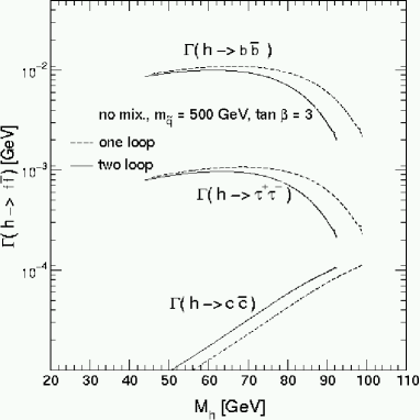
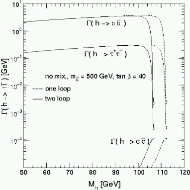
Figure 5.2: $\Gamma(h\to b\bar{b})$, $\Gamma(h\to\tau^{+}\tau^{-})$ and $\Gamma(h\to c\bar{c})$ are shown as a function of $M_{h}$. The Higgs-propagator corrections have been evaluated at the one- and at the two-loop level. The QED, gluon and gluino contributions are included. The other parameters are $\mu=-100\,\,\mathrm{GeV}$, $M_{2}=M_{\rm SUSY}$, $m_{\tilde{g}}=500\,\,\mathrm{GeV}$, $A_{b}=A_{t}$, $\tan\beta\hskip 2.84526pt=3,40$. The result is given in the no-mixing scenario.

     

     

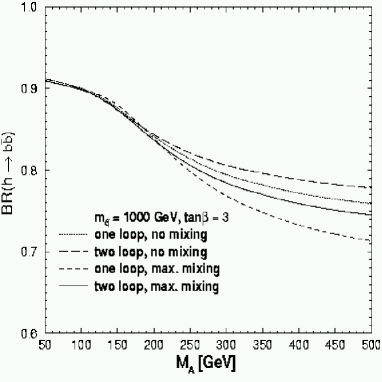
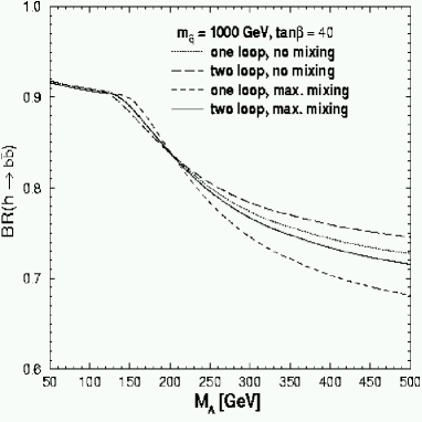
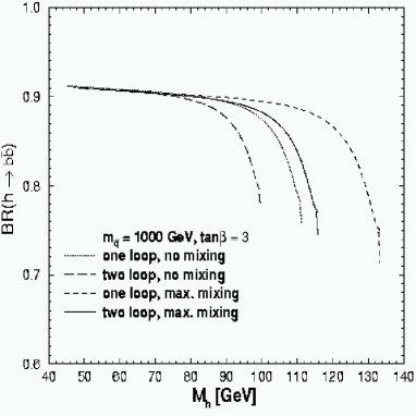
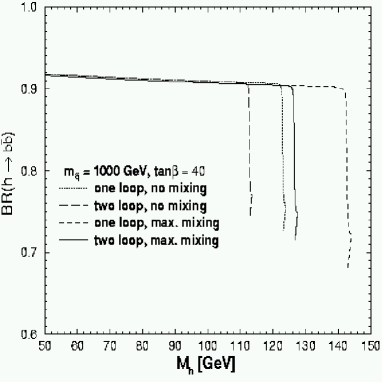
Figure 5.3: ${\rm BR}(h\to b\bar{b})$ is shown as a function of $M_{A}$ and $M_{h}$ for the same settings as in Fig. 5.1. The QED, gluon and gluino contributions are included.

In the low $\tan\beta$ scenario $\Gamma(h\to b\bar{b})$ and $\Gamma(h\to\tau^{+}\tau^{-})$ are lowered at the two-loop level, while $\Gamma(h\to c\bar{c})$ is increased. The decay rate for $h\to b\bar{b}$ is about one and two orders of magnitude larger compared to the ones of $h\to\tau^{+}\tau^{-}$ and $h\to c\bar{c}$, respectively. In the large $\tan\beta$ scenario the shifts are again dominated by the kinematical effect from the different values of $M_{h}$ at the one- and two-loop level. In the maximal-mixing case, which is not plotted here, we find qualitatively the same behavior.

We now turn to the effects of the two-loop corrections to the branching ratios. For not too large values of $M_{h}$, $\Gamma_{\rm tot}$ is strongly dominated by $\Gamma(h\to b\bar{b})$. For large values of $M_{h}$ the decay into gluons becomes more relevant. In Fig. 5.3 we show the branching ratio ${\rm BR}(h\to b\bar{b})$ as a function of $M_{h}$ and $M_{A}$. For values of $M_{A}\;\raisebox{-3.00003pt}{$\stackrel{{\scriptstyle\displaystyle>}}{{\sim}}$}\;250\,\,\mathrm{GeV}$ there is a non-negligible difference between one-loop and two-loop order, where at the two-loop level the branching ratio is slightly enhanced. Compared in terms of $M_{h}$ there is nearly no change for small values of $M_{h}$ in the low and in the high $\tan\beta$ case. Here ${\rm BR}(h\to b\bar{b})$ is changed by less than about 1%, see Fig. 5.3. ${\rm BR}(h\to\tau^{+}\tau^{-})$ is increased by less than about 2%. ${\rm BR}(h\to c\bar{c})$ can be increased at the two-loop level by ${\cal O}(50\%)$, but remains numerically relatively small. For $\tan\beta=40$ the main difference arises at the endpoints of the spectrum, again due to the fact that different Higgs boson masses can be obtained at the one-loop and at the two-loop level. For $\tan\beta=3$, however, also several GeV below the kinematical endpoints there is a sizable effect on ${\rm BR}(h\to b\bar{b})$. Thus, in the experimentally allowed region of $M_{h}$, the two-loop corrections can have an important effect on ${\rm BR}(h\to b\bar{b})$.

5.2.2 Vanishing decay rate for $h\to b\bar{b}$

The search for the Higgs boson, especially at $e^{+}e^{-}$ colliders, often relies on $b$ tagging, since on the one hand the lightest ${\cal CP}$-even Higgs boson decays dominantly into $b\bar{b}$, and on the other hand $b$ tagging can be performed with high efficiency. For some combinations of parameters, however, $\Gamma(h\to b\bar{b})$ can become very small and thus ${\rm BR}(h\to b\bar{b})$ can approach zero as a consequence of large Higgs-boson propagator corrections or large gluino vertex-corrections, making Higgs boson search possibly very difficult for these parameters. Higgs boson searches then have to rely on flavor-independent decay modes. In order to have reliable predictions for these regions of parameter space a full calculation of the one-loop $hb\bar{b}$ vertex corrections, including all ${\cal O}(\alpha)$ contributions, is necessary [111].

Effects of two-loop propagator corrections

We first demonstrate the effect of the two-loop propagator corrections on the values of the parameters, especially of $M_{A}$, for which ${\rm BR}(h\to b\bar{b})$ goes to zero. We also show the impact of the inclusion of the momentum dependence of the Higgs boson self-energies that is often neglected in phenomenological analyses of the decays of the lightest ${\cal CP}$-even Higgs boson.

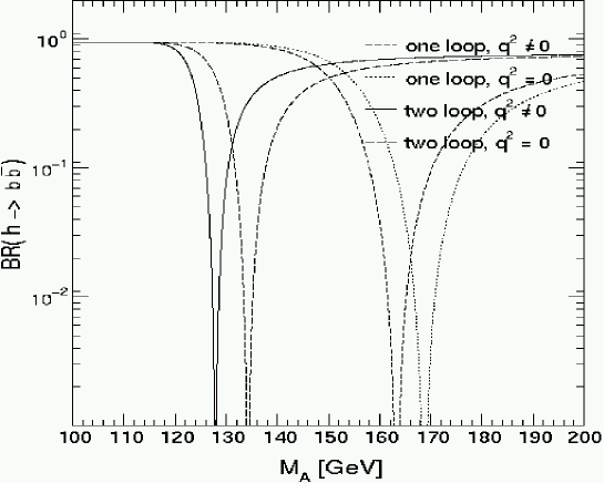
Figure 5.4: ${\rm BR}(h\to b\bar{b})$ is shown as a function of $M_{A}$. The Higgs boson self-energies are evaluated at the one-loop and at the two-loop level with and without momentum dependence (see eq. (5.3)). The other parameters are $\tan\beta=25$, $M_{\rm SUSY}=500\,\,\mathrm{GeV}$, $m_{\tilde{g}}=400\,\,\mathrm{GeV}$, $M_{2}=400\,\,\mathrm{GeV}$, $X_{t}=400\,\,\mathrm{GeV}$, $A_{b}=A_{t}$, $\mu=-1000\,\,\mathrm{GeV}$.

In Fig. 5.4 ${\rm BR}(h\to b\bar{b})$ is shown as a function of $M_{A}$. The Higgs boson self-energies are evaluated at the one-loop and at the two-loop level with and without momentum dependence (see eq. (5.3)). The other parameters are $\tan\beta=25$, $M_{\rm SUSY}=500\,\,\mathrm{GeV}$, $m_{\tilde{g}}=400\,\,\mathrm{GeV}$, $M_{2}=400\,\,\mathrm{GeV}$, $X_{t}=400\,\,\mathrm{GeV}$, $A_{b}=A_{t}$, $\mu=-1000\,\,\mathrm{GeV}$. The inclusion of the two-loop propagator corrections shifts the $M_{A}$ value for which ${\rm BR}(h\to b\bar{b})$ becomes very small by about $-35\,\,\mathrm{GeV}$. The inclusion of the momentum dependence of the Higgs boson self-energies induces another shift of about $-6\,\,\mathrm{GeV}$. In order to have reliable phenomenological predictions for the problematic $M_{A}$ values the two-loop corrections as well as the inclusion of the momentum dependence is necessary. Note that the inclusion of the gluino vertex corrections as well as the purely weak vertex corrections can also have a large impact on the critical $M_{A}$ values.

Effects of ${\cal O}(\alpha_{s}\alpha_{b})$

We now turn to the effects of the additional contributions induced by ${\cal O}(\alpha_{s}\alpha_{b})$ corrections and the corresponding resummation as discussed in Sect. 2.3.4. We recall the tree-level couplings of the lightest ${\cal CP}$-even Higgs boson to the up-type and down-type SM fermions:

$$\Gamma_{h}^{\,u}=\frac{i\,e\,m_{u}}{2\,s_{\mathrm{w}}\,M_{W}}\,\frac{-\cos\alpha\hskip 2.84526pt}{\sin\beta}\,,\hskip 56.9055pt\Gamma_{h}^{\,d}=\frac{i\,e\,m_{d}}{2\,s_{\mathrm{w}}\,M_{W}}\,\frac{\sin\alpha\hskip 2.84526pt}{\cos\beta\hskip 2.84526pt}\,.$$ (5.45)

The main source (besides the SM QCD corrections and the Higgs boson propagator corrections) modifying the $hb\bar{b}$ and $h\tau^{+}\tau^{-}$ vertices are the corrections modifying the relation between the bottom quark or $\tau$ lepton mass and the corresponding Yukawa couplings.

The potentially large corrections to the $\Gamma_{h}^{\,d}$ couplings come from the $\tan\beta$-enhanced threshold effects in the relation between the down-type fermion mass and the corresponding Yukawa coupling [43], already mentioned in Sect. 5.1.3. A simple way to take into account these effects is to employ the effective Lagrangian formalism of Refs. [44, 55], see Sect. 2.3.4, where the coupling of the lightest Higgs boson to down-type fermions (expressed through the fermion mass) can be written as

$$\left(\Gamma_{h}^{\,d}\right)_{\rm eff}=\frac{i\,e\,m_{d}}{2\,s_{\mathrm{w}}\,M_{W}}\,\frac{\sin\alpha_{\rm eff}}{\cos\beta\hskip 2.84526pt}\,\left[1-\frac{\Delta m_{d}}{1+\Delta m_{d}}\,(1+\cot\alpha_{\rm eff}\,\cot\beta)\right]\,,$$ (5.46)

where $\Delta m_{d}$ contains (as described in Sect. 2.3.4) the $\tan\beta$-enhanced terms, and other subleading (i.e. non $\tan\beta$-enhanced) corrections have been omitted. In the case of the coupling to the bottom quarks, the leading contributions to $\Delta m_{b}$ are of ${\cal O}(\alpha_{s})$ and ${\cal O}(\alpha_{t})$, coming from diagrams with sbottom–gluino and stop–chargino loops, respectively. In the case of the $\tau$ leptons, the leading contributions are of ${\cal O}(\alpha_{\tau})$, coming from sneutrino–chargino loops. The terms containing $\Delta m_{d}$ in eq. (5.46) may be relevant for large $\tan\beta$ and moderate values of $M_{A}$. When $M_{A}$ is much bigger than $M_{Z}$, the product $\cot\alpha_{\rm eff}\,\cot\beta$ tends to $-1$, and the SM limit is again recovered.

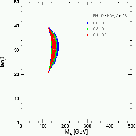
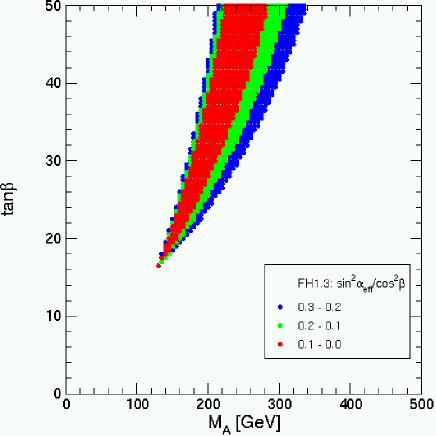
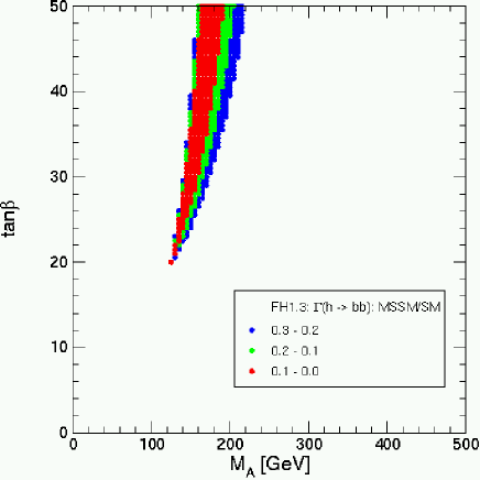
Figure 5.5: Regions of significant suppression of the coupling of $h$ to down-type fermions in the $M_{A}$–$\tan\beta$-plane within the “small $\alpha_{\rm eff}$” benchmark scenario. The upper left plot shows the ratio $\sin^{2}\alpha_{\rm eff}/\cos^{2}\beta\hskip 2.84526pt$ as evaluated with FeynHiggs1.0 (i.e. without ${\cal O}(\alpha_{b}\alpha_{s})$ and ${\cal O}(\alpha_{b}(\alpha_{s}\tan\beta)^{n})$ corrections), while the upper right plot shows the same quantity as evaluated with FeynHiggs1.3 (i.e. including these corrections). The plot in the lower row shows the ratio $\Gamma(h\rightarrow b\bar{b})_{\rm MSSM}\,/\,\Gamma(h\rightarrow b\bar{b})_{\rm SM}$, i.e. the partial width for $h\to b\bar{b}$ normalized to its SM value, where the other term in eq. (5.46) and further genuine loop corrections are taken into account (see text).

The effects of the higher-order corrections to the couplings of the lightest Higgs boson to the down-type fermions appear very pronounced in the “small $\alpha_{\rm eff}$” scenario [53], see the Appendix.

In the upper row of Fig. 5.5 we show the ratio $\sin^{2}\alpha_{\rm eff}/\cos^{2}\beta\hskip 2.84526pt$ in the $M_{A}$–$\tan\beta$ plane, evaluated in the “small $\alpha_{\rm eff}$” scenario. As explained above, replacing $\alpha$ by $\alpha_{\rm eff}$ in the tree-level couplings of eq. (5.45) gives rise to regions in the $M_{A}$–$\tan\beta$ plane where the effective coupling of the lightest Higgs boson to the down-type fermions is significantly suppressed with respect to the Standard Model. The region of significant suppression of $\sin^{2}\alpha_{\rm eff}/\cos^{2}\beta\hskip 2.84526pt$ as evaluated without the inclusion of the sbottom corrections beyond one-loop order, is shown in the upper left plot. The upper right plot shows the corresponding result as evaluated with FeynHiggs2.1, where the ${\cal O}(\alpha_{b}\alpha_{s})$ and ${\cal O}(\alpha_{b}(\alpha_{s}\tan\beta)^{n})$ corrections as well as the new ${\cal O}(\alpha_{t}^{2})$ ones are included. The new corrections are seen to have a drastic impact on the region where $\sin^{2}\alpha_{\rm eff}/\cos^{2}\beta\hskip 2.84526pt$ is small. While without the new corrections a suppression of 70% or more occurs only in a small area of the $M_{A}$–$\tan\beta$-plane for $20\;\raisebox{-3.00003pt}{$\stackrel{{\scriptstyle\displaystyle<}}{{\sim}}$}\;\tan\beta\;\raisebox{-3.00003pt}{$\stackrel{{\scriptstyle\displaystyle<}}{{\sim}}$}\;40$ and $100\,\,\mathrm{GeV}\;\raisebox{-3.00003pt}{$\stackrel{{\scriptstyle\displaystyle<}}{{\sim}}$}\;M_{A}\;\raisebox{-3.00003pt}{$\stackrel{{\scriptstyle\displaystyle<}}{{\sim}}$}\;200\,\,\mathrm{GeV}$, the region where $\sin^{2}\alpha_{\rm eff}/\cos^{2}\beta\hskip 2.84526pt$ is very small becomes much larger once these corrections are included. It now reaches from $\tan\beta\;\raisebox{-3.00003pt}{$\stackrel{{\scriptstyle\displaystyle>}}{{\sim}}$}\;15$ to $\tan\beta>50$, and from $M_{A}\;\raisebox{-3.00003pt}{$\stackrel{{\scriptstyle\displaystyle>}}{{\sim}}$}\;100\,\,\mathrm{GeV}$ to $M_{A}\;\raisebox{-3.00003pt}{$\stackrel{{\scriptstyle\displaystyle<}}{{\sim}}$}\;350\,\,\mathrm{GeV}$. The main reason for the change is that the one-loop ${\cal O}(\alpha_{b})$ corrections to the Higgs-boson mass matrix, which for large $\tan\beta$ would prevent $\alpha_{\rm eff}$ from going to zero, are heavily suppressed by the resummation of the ${\cal O}(\alpha_{b}(\alpha_{s}\tan\beta)^{n})$ corrections in the bottom Yukawa coupling. This kind of suppression depends strongly on the chosen MSSM parameters, and especially on the sign of $\mu$.

In order to interpret the physical impact of the effective coupling shown in the upper row of Fig. 5.5, the $\Delta m_{d}$ terms in eq. (5.46) as well as further genuine loop corrections occurring in the $h\to b\bar{b}$ process have to be taken into account as described in Sect. 5.1.3. The effect of these contributions can be seen from the plot in the lower row of Fig. 5.5, where the ratio $\Gamma(h\rightarrow b\bar{b})_{\rm MSSM}\,/\,\Gamma(h\rightarrow b\bar{b})_{\rm SM}$ is shown, which has been evaluated by including all terms of eq. (5.46) as well as all further corrections given in eq. (5.30). The region where the partial width $\Gamma(h\rightarrow b\bar{b})$ within the MSSM is suppressed compared to its SM value is seen to be somewhat reduced and shifted towards smaller values of $M_{A}$ as compared to the region where $\sin^{2}\alpha_{\rm eff}/\cos^{2}\beta\hskip 2.84526pt$ is small.

5.2.3 Effects of the gluino vertex corrections

In this subsection we focus on the effect of the gluino-exchange contribution to the $hf\bar{f}$ vertex corrections in a more general way, i.e. for parameters where $hf\bar{f}$ does not go to zero.

     

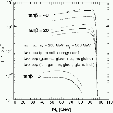
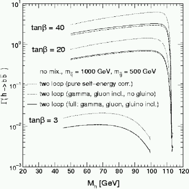
Figure 5.6: $\Gamma(h\to b\bar{b})$ is shown as a function of $M_{h}$ for three values of $\tan\beta$. The Higgs-propagator corrections have been evaluated at the two-loop level in the no-mixing scenario. The dotted curves shows the results containing only the pure self-energy corrections. The results given in the dashed curves in addition contain the QED correction and the gluon-exchange contribution. The solid curves show the full result, including also the gluino correction. The other parameters are $\mu=-100\,\,\mathrm{GeV}$, $M_{2}=m_{\tilde{q}}$, $A_{b}=A_{t}$.

     

Figure 5.7: $\Gamma(h\to b\bar{b})$ is shown as a function of $\mu$ for $\tan\beta\hskip 2.84526pt=20$ and two different values of $m_{\tilde{g}}$ in the no-mixing and the maximal-mixing scenario. The other parameters are $m_{\tilde{q}}=500\,\,\mathrm{GeV}$, $M_{2}=500\,\,\mathrm{GeV}$, $A_{b}=A_{t}$, $M_{A}=100\,\,\mathrm{GeV}$.

Fig. 5.6 shows $\Gamma(h\to b\bar{b})$ in three steps of accuracy: the dotted curves contain only the pure self-energy correction, the dashed curves contain in addition the QED and the gluon-exchange correction. The solid curves show the full results including also the gluino-exchange correction. The results are shown for $X_{t}=0$ (no mixing), $\mu=-100\,\,\mathrm{GeV}$, $m_{\tilde{g}}=500\,\,\mathrm{GeV}$, $m_{\tilde{q}}=200,1000\,\,\mathrm{GeV}$, in the left and right part of Fig. 5.6, respectively. For $\tan\beta$, three values have been chosen: $\tan\beta=3,20,40$.

The left plot of Fig. 5.6 corresponds to a small soft SUSY-breaking scale, $m_{\tilde{q}}=200\,\,\mathrm{GeV}$. The effect of the gluon contribution is large and negative, the effect of the QED correction is small. For this combination of $m_{\tilde{g}}$, $m_{\tilde{q}}$ and $\mu$ the effect of the gluino correction is large and positive, as can be seen from the transition from the dashed to the solid curves. For $\tan\beta\hskip 2.84526pt=40$ it nearly compensates the gluon effect, for $\tan\beta=20$ it amounts up to 20% of the gluonic correction, while for $\tan\beta=3$ the gluino-exchange contribution is negligible. Note that we have chosen a relatively small value of $\mu$, $\mu=-100\,\,\mathrm{GeV}$. For larger values of $|\mu|$ even larger corrections can be obtained. Hence neglecting the gluino-exchange correction in the large $\tan\beta$ scenario can lead to results which deviate by 50% from the full ${\cal O}(\alpha_{s})$ calculation (see also Sect. 5.1.4). The right plot of Fig. 5.6 corresponds to $m_{\tilde{q}}=1000\,\,\mathrm{GeV}$. The gluino-exchange effects are still visible, but much smaller than for $m_{\tilde{q}}=200\,\,\mathrm{GeV}$. The same observation has already been made in Ref. [11]. For $X_{t}=2m_{\tilde{q}}$ (maximal mixing) we find qualitatively the same behavior for the gluino-exchange corrections as for $X_{t}=0$.

In Fig. 5.7 the pure gluino-exchange effect is shown as a function of $\mu$. This effect increases with rising $m_{\tilde{g}}$ and $|\mu|$, where for negative (positive) $\mu$ there is an enhancement (a decrease) in $\Gamma(h\to b\bar{b})$. The size of the gluino-exchange contribution also depends on $M_{A}$, where larger effects correspond to smaller values of $M_{A}$, see also Ref. [11]. The small difference between the curves where the decay rate has been calculated without gluino contribution is due to the variation of $M_{h}$ induced by different values of $m_{\tilde{g}}$ which enters at ${\cal O}(\alpha\alpha_{s})$. Fig. 5.7 demonstrates again that neglecting the gluino contribution in the fermion decay rates can yield (strongly) misleading results.

As a final remark, one should note that the gluino exchange contribution has only a relatively small impact on ${\rm BR}(h\to b\bar{b})$. However, it can have a large influence on ${\rm BR}(h\to\tau^{+}\tau^{-})$ or ${\rm BR}(h\to WW^{*})$. Both branching ratios are expected to be measurable at the per-cent level, see Tab. 1.3. While the Higgs-propagator contributions are universal corrections that affect $\Gamma(h\to b\bar{b})$ and $\Gamma(h\to\tau^{+}\tau^{-},h\to WW^{*})$ in the same way (i.e. the influence on the effective coupling is the same in both cases), the gluino corrections, which influence only $\Gamma(h\to b\bar{b})$, can lead to a different behavior of the decay widths. This has been analyzed in the mSUGRA, GMSB and AMSB scenario in Refs. [115, 116].

5.2.4 The $\alpha_{\rm eff}$-approximation

Finally, we investigate the quality of the $\alpha_{\rm eff}$-approximation. In Fig. 5.8 we display the relative difference between the full result (5.18) and the $\alpha_{\rm eff}$ result, where the external momentum of the Higgs self-energies has been neglected, see eq. (5.19). The relative difference $\Delta\Gamma(h\to b\bar{b})=(\Gamma^{\rm full}(h\to b\bar{b})-\Gamma^{\alpha_{\rm eff}}(h\to b\bar{b}))/\Gamma^{\rm full}(h\to b\bar{b})$ is shown as a function of $M_{A}$ for $m_{\tilde{q}}=1000\,\,\mathrm{GeV}$ and for three values of $\tan\beta$ in the no mixing and the maximal mixing scenario. Large deviations occur only in the region $100\,\,\mathrm{GeV}\;\raisebox{-3.00003pt}{$\stackrel{{\scriptstyle\displaystyle<}}{{\sim}}$}\;M_{A}\;\raisebox{-3.00003pt}{$\stackrel{{\scriptstyle\displaystyle<}}{{\sim}}$}\;150\,\,\mathrm{GeV}$, especially for large $\tan\beta$. In this region of parameter space the values of $M_{h}$ and $M_{H}$ are very close to each other. This results in a high sensitivity to small deviations in the Higgs boson self-energies entering the Higgs-boson mass matrix eq. (2.85). Another source of differences between the full and the approximate calculation is the threshold $M_{A}=2\,m_{t}=350\,\,\mathrm{GeV}$ in the one-loop contribution, originating from the top-loop diagram in the $A$ self-energy, see Ref. [99] for more details. Here the deviation can amount up to 6%. This threshold is only present in the pure on-shell renormalization (see also Sect. 2.3.4), which has been used for these plots. Making use of the hybrid $\overline{\rm{DR}}$/on-shell renormalization (as incorporate in the latest version of FeynHiggs), these thresholds are absent.

In Fig. 5.9 we compare the $\alpha_{\rm eff}$ result (5.19) with the $\alpha_{\rm eff}{\rm(approx)}$ result (5.20), where the Higgs boson self-energies have been approximated by the compact analytical expression obtained in Ref. [17]. Figure 5.9 displays the relative difference in the effective mixing angles, $(\sin\alpha_{\rm eff}-\sin\alpha_{\rm eff}{\rm(approx)})/\sin\alpha_{\rm eff}$. Via eq. (5.14) $\sin\alpha_{\rm eff}$ directly determines the decay width $\Gamma(h\to b\bar{b})$. The result is shown for $m_{\tilde{q}}=1000\,\,\mathrm{GeV}$, for three values of $\tan\beta$ in the minimal and the maximal mixing scenario. Apart from the region around $M_{A}\approx 120\,\,\mathrm{GeV}$ (compare Fig. 5.8) both effective angles agree better than 3% with each other.

Concerning the comparison of the $\alpha_{\rm eff}$-approximations in terms of $M_{h}$ (which is not plotted here), due to the neglected external momentum or the neglected subdominant one- or two-loop terms, $M_{h}$ receives a slight shift. Besides this kinematical effect, the decay rate is approximated rather well for most of the $M_{h}$ values: independently of $m_{\tilde{q}}$, the differences stay mostly below 2–4%, for the no-mixing case as well as for the maximal-mixing case. Only at the endpoints of the spectrum, due to the different Higgs-boson mass values, the difference is not negligible.

     

Figure 5.8: $\Delta\Gamma(h\to b\bar{b})=(\Gamma^{\rm full}(h\to b\bar{b})-\Gamma^{\alpha_{\rm eff}}(h\to b\bar{b}))/\Gamma^{\rm full}(h\to b\bar{b})$ is shown as a function of $M_{A}$ for three values of $\tan\beta$. The QED, gluon- and gluino-contributions are neglected here. The other parameters are $\mu=-100\,\,\mathrm{GeV}$, $M_{2}=m_{\tilde{q}}$, $m_{\tilde{g}}=500\,\,\mathrm{GeV}$, $A_{b}=A_{t}$, $\tan\beta\hskip 2.84526pt=3,20,40$. $X_{t}$ has been set to $X_{t}=0$ (no mixing) or $X_{t}=2m_{\tilde{q}}$ (maximal mixing).

     

Figure 5.9: The relative difference $(\sin\alpha_{\rm eff}-\sin\alpha_{\rm eff}{\rm(approx)})/\sin\alpha_{\rm eff}$ (see eqs. (5.19) and (5.20)) is shown as a function of $M_{A}$ for three values of $\tan\beta$ for $X_{t}=0$ (no mixing) and $X_{t}=2m_{\tilde{q}}$ (maximal mixing). The other parameters are chosen as in Fig. 5.8.

Chapter 6 Conclusions

We have reviewed the current status of higher-order corrections in the MSSM Higgs sector. This comprises the corrections to the Higgs boson masses in the real and complex MSSM, the existing corrections to Higgs boson production cross sections at the LC as well as corrections to Higgs boson decays to SM fermions.

Concerning Higgs boson masses and couplings in the MSSM with real parameters, the higher-order corrections are known to be huge. The corrections described in this report lower the intrinsic error due to unknown higher-order corrections down to about $\sim 3\,\,\mathrm{GeV}$ for the lightest Higgs boson mass. Likewise a precision at the per-cent level for the couplings can be reached. In the case of the MSSM with complex parameters, uncertainties of more than $\sim 5\,\,\mathrm{GeV}$ for the lightest Higgs boson mass have been eliminated. The effects of the full one-loop corrections have been shown to be substantial for all Higgs boson masses and couplings. We have investigated the higher-order contributions to Higgs boson production channels at the LC and found corrections of up to $\sim 20\%$ for the channel $e^{+}e^{-}\to hZ$. In the $WW$ fusion channel especially the non-decoupling behavior of the heavy ${\cal CP}$-even Higgs boson has been investigated. Taking loop corrections into account the reach of the LC could be extended by up to $\sim 200\,\,\mathrm{GeV}$. Concerning the Higgs boson decays to SM fermions, we have shown that the corrections arising in the Feynman-diagrammatic approach are subtantial and have to be taken into account in an accurate analysis. This holds especially for gluino-loop corrections for the decay $h\to b\bar{b}$.

To summarize, in all investigated cases the higher-order corrections are substantial and must not be neglected in phenomenological analyses. Once a MSSM-like Higgs boson will have been discovered, and the corresponding quantities like masses, couplings and production cross sections will be measured at the LHC and (hopefully) furtheron at the LC, it will be mandatory to have even more precise evaluations at hand. In view of the complexity of these calculations in the past, and the time needed to perform them, further higher-order corrections will have to be evaluated continously in the future. Only then the required precision will be available at the same time as the experimental data will be determined from the collider experiments.

At the same time it will be necessary not only to improve on the higher-order corrections but also on the reduction of the parametric uncertainties due to the imperfect knowledge of the input parameters. This is especially true for the top quark mass. Here certainly the LC precision will be necessary to match even the anticipated LHC precision in $M_{h}$.

The tasks for theorist described above are huge. However, it still seems to be possible to achieve the required calculations, provided that there is enough financial and man power support from the whole community [117]. Then (but only then) it can be possible that theoretical and experimental high-energy physics has a bright future.

Appendix

For our numerical results, the following values of the SM parameters are used (all other quark and lepton masses are negligible):

$$G_{F} =1.16639\times 10^{-5}, \quad m_{\tau} =1.777\,\,\mathrm{GeV},$$ (1)

$$M_{W} =80.450\,\,\mathrm{GeV}, m_{t} =174.3\,\,\mathrm{GeV},$$

$$M_{Z} =91.1875\,\,\mathrm{GeV}, m_{b} =4.25\,\,\mathrm{GeV},$$

$$\Gamma_{Z} =2.4952\,\,\mathrm{GeV}, m_{c} =1.5\,\,\mathrm{GeV}.$$

For our numerical evaluation we mostly rely on four benchmark scenarios that have been defined in Ref. [53] for Higgs boson searches at hadron colliders and beyond. The four benchmark scenarios are (more details can be found in Ref. [53])

• the “$m_{h}^{\rm max}$” scenario, which yields a maximum value of $M_{h}$ for given $M_{A}$ and $\tan\beta$,

  $$m_{t}=174.3\,\,\mathrm{GeV},\quad M_{\rm SUSY}=1\,\,\mathrm{TeV},\quad\mu=200\,\,\mathrm{GeV},\quad M_{2}=200\,\,\mathrm{GeV},$$ (2)

  $$X_{t}=2\,M_{\rm SUSY},\quad A_{\tau}=A_{b}=A_{t},\quad m_{\tilde{g}}=0.8\,M_{\rm SUSY}\,,$$

• the “no-mixing” scenario, with no mixing in the $\tilde{t}$ sector,

  $$m_{t}=174.3\,\,\mathrm{GeV},\quad M_{\rm SUSY}=2\,\,\mathrm{TeV},\quad\mu=200\,\,\mathrm{GeV},\quad M_{2}=200\,\,\mathrm{GeV},$$

  $$X_{t}=0,\quad A_{\tau}=A_{b}=A_{t},\quad m_{\tilde{g}}=0.8\,M_{\rm SUSY}\,,$$ (3)

• the “gluophobic-Higgs” scenario, with a suppressed $ggh$ coupling,

  $$m_{t}=174.3\,\,\mathrm{GeV},\quad M_{\rm SUSY}=350\,\,\mathrm{GeV},\quad\mu=300\,\,\mathrm{GeV},\quad M_{2}=300\,\,\mathrm{GeV},$$

  $$X_{t}=-750\,\,\mathrm{GeV},\quad A_{\tau}=A_{b}=A_{t},\quad m_{\tilde{g}}=500\,\,\mathrm{GeV}\,,$$ (4)

• the “small-$\alpha_{\rm eff}$” scenario, with possibly reduced decay rates for $h\to b\bar{b}$ and $h\to\tau^{+}\tau^{-}$,

  $$m_{t}=174.3\,\,\mathrm{GeV},\quad M_{\rm SUSY}=800\,\,\mathrm{GeV},\quad\mu=2.5\,M_{\rm SUSY},\quad M_{2}=500\,\,\mathrm{GeV},$$

  $$X_{t}=-1100\,\,\mathrm{GeV},\quad A_{\tau}=A_{b}=A_{t},\quad m_{\tilde{g}}=500\,\,\mathrm{GeV}\,.$$ (5)

As explained above, for the sake of simplicity, $M_{\rm SUSY}$ is chosen as a common soft SUSY-breaking parameter for all three generations.

Acknowledgements

I thank all my collaborators with whom I have worked on the various calculations presented here. These are O. Brein, M. Carena, G. Degrassi, M. Frank, H. Haber, T. Hahn, W. Hollik, J. Rosiek, P. Slavich, C. Wagner, and G. Weiglein. Furthermore, I thank S. Dawson, S. Dittmaier, U. Nierste, H. Rzehak, and M. Spira for helpful discussions. I am also gratefull to S. Dittmaier, W. Hollik and G. Weiglein for a critical reading of the manuscript. Finally, I thank I. Campos for inspirational as well as W. Lagavulin and W. Laphroigh for spiritual encouragement. This work has been supported by the European Community’s Human Potential Programme under contract HPRN-CT-2000-00149 Physics at Colliders.

Bibliography

-
[1]
H.P. Nilles,
Phys. Rep. 110 (1984) 1;
H.E. Haber and G.L. Kane, Phys. Rep. 117, (1985) 75;
R. Barbieri, Riv. Nuovo Cim. 11, (1988) 1. -
[2]
G. Kane, C. Kolda and J. Wells,
Phys. Rev. Lett. 70 (1993) 2686,
hep-ph/9210242;
J. Espinosa and M. Quirós, Phys. Rev. Lett. 81 (1998) 516, hep-ph/9804235. - [3] P. Azzi et al. [CDF Collaborattion, D0 Collaboration], hep-ex/0404010.
- [4] The Top Averaging Collaboration, L. Demortier et al., FERMILAB-TM-2084 (1999).
- [5] S. Heinemeyer, W. Hollik and G. Weiglein, Eur. Phys. Jour. C 9 (1999) 343, hep-ph/9812472.
- [6] S. Heinemeyer, W. Hollik and G. Weiglein, JHEP 0006 (2000) 009, hep-ph/9909540.
- [7] G. Degrassi, S. Heinemeyer, W. Hollik, P. Slavich and G. Weiglein, Eur. Phys. Jour. C 28 (2003) 133, hep-ph/0212020.
-
[8]
J. Ellis, G. Ridolfi and F. Zwirner,
Phys. Lett. B 257, 83 (1991);
Y. Okada, M. Yamaguchi and T. Yanagida, Prog. Theor. Phys. 85, 1 (1991);
H. Haber and R. Hempfling, Phys. Rev. Lett. 66, 1815 (1991). - [9] A. Brignole, Phys. Lett. B 281 (1992) 284.
- [10] P. Chankowski, S. Pokorski and J. Rosiek, Phys. Lett. B 286 (1992) 307; Nucl. Phys. B 423 (1994) 437, hep-ph/9303309.
- [11] A. Dabelstein, Nucl. Phys. B 456 (1995) 25, hep-ph/9503443; Z. Phys. C 67 (1995) 495, hep-ph/9409375.
- [12] R. Hempfling and A. Hoang, Phys. Lett. B 331 (1994) 99, hep-ph/9401219.
- [13] J. Casas, J. Espinosa, M. Quirós and A. Riotto, Nucl. Phys. B 436 (1995) 3, E: ibid. B 439 (1995) 466, hep-ph/9407389.
-
[14]
M. Carena, J. Espinosa, M. Quirós and C. Wagner,
Phys. Lett. B 355 (1995) 209,
hep-ph/9504316;
M. Carena, M. Quirós and C. Wagner, Nucl. Phys. B 461 (1996) 407, hep-ph/9508343. - [15] H. Haber, R. Hempfling and A. Hoang, Z. Phys. C 75 (1997) 539, hep-ph/9609331.
- [16] S. Heinemeyer, W. Hollik and G. Weiglein, Phys. Rev. D 58 (1998) 091701, hep-ph/9803277; Phys. Lett. B 440 (1998) 296, hep-ph/9807423.
- [17] S. Heinemeyer, W. Hollik and G. Weiglein, Phys. Lett. B 455 (1999) 179, hep-ph/9903404.
-
[18]
R. Zhang, Phys. Lett. B 447 (1999) 89,
hep-ph/9808299;
J. Espinosa and R. Zhang, JHEP 0003 (2000) 026, hep-ph/9912236. - [19] G. Degrassi, P. Slavich and F. Zwirner, Nucl. Phys. B 611 (2001) 403, hep-ph/0105096.
- [20] J. Espinosa and R. Zhang, Nucl. Phys. B 586 (2000) 3, hep-ph/0003246.
- [21] A. Brignole, G. Degrassi, P. Slavich and F. Zwirner, Nucl. Phys. B 631 (2002) 195, hep-ph/0112177.
- [22] A. Brignole, G. Degrassi, P. Slavich and F. Zwirner, Nucl. Phys. B 643 (2002) 79, hep-ph/0206101.
- [23] S. Heinemeyer, W. Hollik, H. Rzehak and G. Weiglein, in preparation.
- [24] G. Degrassi, A. Dedes and P. Slavich, Nucl. Phys. B 672 (2003) 144, hep-ph/0305127.
- [25] S. Martin, Phys. Rev. D 65 (2002) 116003, hep-ph/0111209; Phys. Rev. D 66 (2002) 096001, hep-ph/0206136; Phys. Rev. D 67 (2003) 095012, hep-ph/0211366; Phys. Rev. D 68 075002 (2003), hep-ph/0307101; hep-ph/0312092; hep-ph/0405022.
-
[26]
A. Pilaftsis,
Phys. Rev. D 58 (1998) 096010,
hep-ph/9803297;
A. Pilaftsis, Phys. Lett. B 435 (1998) 88, hep-ph/9805373. -
[27]
D. Demir,
Phys. Rev. D 60 (1999) 055006,
hep-ph/9901389;
S. Choi, M. Drees and J. Lee, Phys. Lett. B 481 (2000) 57, hep-ph/0002287. - [28] A. Pilaftsis and C. Wagner, Nucl. Phys. B 553 (1999) 3, hep-ph/9902371.
- [29] M. Carena, J. Ellis, A. Pilaftsis and C. Wagner, Nucl. Phys. B 586 (2000) 92, hep-ph/0003180.
- [30] T. Ibrahim and P. Nath, Phys. Rev. D 63 (2001) 035009, hep-ph/0008237; Phys. Rev. D 66 (2002) 015005, hep-ph/0204092.
- [31] S. Heinemeyer, Eur. Phys. Jour. C 22 (2001) 521, hep-ph/0108059.
- [32] M. Frank, S. Heinemeyer, W. Hollik and G. Weiglein, hep-ph/0212037, appeared in the proceedings of SUSY02, DESY, Hamburg, Germany, July 2002.
- [33] M. Frank, S. Heinemeyer, W. Hollik and G. Weiglein, in preparation.
- [34] M. Carena et al., [Higgs Working Group Collaboration], hep-ph/0010338.
-
[35]
ATLAS Collaboration,
Detector and Physics Performance Technical Design Report,
CERN/LHCC/99-15 (1999), see:
atlasinfo.cern.ch/Atlas/GROUPS/PHYSICS/TDR/access.html ;
CMS Collaboration, see:
cmsinfo.cern.ch/Welcome.html/CMSdocuments/CMSplots . - [36] M. Dührssen, S. Heinemeyer, H. Logan, D. Rainwater, G. Weiglein and D. Zeppenfeld, hep-ph/0406323.
- [37] J. Aguilar-Saavedra et al., TESLA TDR Part 3: “Physics at an Linear Collider”, hep-ph/0106315, see: tesla.desy.de/tdr .
-
[38]
K. Desch and N. Meyer,
LC-PHSM-2001-025, see:
www.desy.de/lcnotes ;
K. Desch, private communication. - [39] J.-C. Brient, LC-PHSM-2004-002, see: www-flc.desy.de/lcnotes .
- [40] T. Barklow, hep-ph/0312268.
-
[41]
A. Djouadi, W. Kilian, M. Mühlleitner and P. Zerwas,
Eur. Phys. Jour. C 10 (1999) 45,
hep-ph/9903229;
C. Castanier, P. Gay, P. Lutz and J. Orloff, hep-ex/0101028. - [42] J. Gunion, H. Haber, G. Kane and S. Dawson, The Higgs Hunter’s Guide, Addison-Wesley, 1990.
-
[43]
T. Banks,
Nucl. Phys. B 303 (1988) 172;
L. Hall, R. Rattazzi and U. Sarid, Phys. Rev. D 50 (1994) 7048, hep-ph/9306309;
R. Hempfling, Phys. Rev. D 49 (1994) 6168;
M. Carena, M. Olechowski, S. Pokorski and C. Wagner, Nucl. Phys. B 426 (1994) 269, hep-ph/9402253. - [44] M. Carena, D. Garcia, U. Nierste and C. Wagner, Nucl. Phys. B 577 (2000) 577, hep-ph/9912516.
- [45] B. Allanach, A. Djouadi, J. Kneur, W. Porod and P. Slavich, hep-ph/0406166.
- [46] M. Diaz and H. Haber, Phys. Rev. D 45 (1992) 4246.
- [47] M. Frank, PhD thesis, university of Karlsruhe, 2002.
-
[48]
S. Heinemeyer, W. Hollik and G. Weiglein,
Comp. Phys. Comm. 124 2000 76,
hep-ph/9812320;
hep-ph/0002213.
The codes are accessible at www.feynhiggs.de . - [49] M. Frank, S. Heinemeyer, W. Hollik and G. Weiglein, hep-ph/0202166.
-
[50]
W. Siegel,
Phys. Lett. B 84 (1979) 193;
D. Capper, D. Jones, and P. van Nieuwenhuizen, Nucl. Phys. B 167 (1980) 479. - [51] S. Heinemeyer, D. Stöckinger and G. Weiglein, in preparation.
- [52] A. Freitas and D. Stöckinger, Phys. Rev. D 66, 095014 (2002), hep-ph/0205281; hep-ph/0210372.
- [53] M. Carena, S. Heinemeyer, C. Wagner and G. Weiglein, hep-ph/9912223; Eur. Phys. J. C 26 (2003) 601, hep-ph/0202167.
- [54] J. Espinosa and I. Navarro, Nucl. Phys. B 615 (2001) 82, hep-ph/0104047.
- [55] H. Eberl, K. Hidaka, S. Kraml, W. Majerotto and Y. Yamada, Phys. Rev. D 62 (2000) 055006, hep-ph/9912463.
-
[56]
[LEP Higgs working group],
hep-ex/0107030;
hep-ex/0107031;
LHWG Note 2001-4,
see:
lephiggs.web.cern.ch/LEPHIGGS/papers . - [57] B. Allanach et al., Eur. Phys. Jour. C 25 (2002) 113, hep-ph/0202233.
- [58] A. Quadt, private communication.
- [59] M. Carena, H. Haber, S. Heinemeyer, W. Hollik, C. Wagner and G. Weiglein, Nucl. Phys. B 580 (2000) 29, hep-ph/0001002.
- [60] [LEP Higgs working group], Phys. Lett. B 565 (2003) 61, hep-ex/0306033.
- [61] S. Heinemeyer, W. Hollik and G. Weiglein, hep-ph/9910283.
- [62] S. Heinemeyer, S. Kraml, W. Porod and G. Weiglein, JHEP 0309 (2003) 075, hep-ph/0306181.
-
[63]
G. Weiglein et al. [LHC/LC study group],
in preparation, see:
www.cpt.dur.ac.uk/georg/lhclc . - [64] Part. Data Group, Phys. Rev. D 66 (2002) 010001.
-
[65]
M. Winter,
talk given at the LHC/LC study group meeting, CERN,
July 2002, see:
www.cpt.dur.ac.uk/georg/lhclc . - [66] J. Erler, S. Heinemeyer, W. Hollik, G. Weiglein and P. Zerwas, Phys. Lett. B 486 (2000) 125; hep-ph/0005024.
- [67] T. Hahn, S. Heinemeyer and G. Weiglein, Nucl. Phys. B 652 (2003), 229, hep-ph/0211204; Nucl. Phys. Proc. Suppl. 116, 336 (2003) hep-ph/0211384.
- [68] A. Hoang, Applications of Two-Loop Calculations in the Standard Model and its Minimal Supersymmetric Extension, PhD thesis, Universität Karlsruhe, Shaker Verlag, Aachen 1995.
- [69] A. Hoang et al., Eur. Phys. Jour. C 3 (2000) 1, hep-ph/0001286.
- [70] S. Heinemeyer and G. Weiglein, hep-ph/0012364.
- [71] E. Gross, S. Heinemeyer, K. Desch, G. Weiglein and L. Zivkovic, hep-ph/0406322.
-
[72]
R. Lafaye, T. Plehn and D. Zerwas,
hep-ph/0404282;
P. Wienemann, talk given at the LCWS Paris, April 2004, see:
agenda.cern.ch/fullAgenda.php?ida=a04172#s15 . - [73] T. Hahn, S. Heinemeyer, W. Hollik and G. Weiglein, in preparation. The code is accessible via www.feynhiggs.de .
-
[74]
J. Küblbeck, M. Böhm, and A. Denner,
Comput. Phys. Commun. 60 (1990) 165;
T. Hahn, Comput. Phys. Commun. 140 (2001) 418, hep-ph/0012260. - [75] T. Hahn and C. Schappacher, Comput. Phys. Commun. 143 (2002) 54, hep-ph/0105349.
- [76] T. Hahn and M. Pérez-Victoria, Comput. Phys. Commun. 118 (1999) 153, hep-ph/9807565.
- [77] F. del Aguila, A. Culatti, R. Munoz Tapia and M. Perez-Victoria, Nucl. Phys. B 537 (1999) 561, hep-ph/9806451.
- [78] V. Barger, T. Falk, T. Han, J. Jiang, T. Li and T. Plehn, Phys. Rev. D 64 (2001) 056007, hep-ph/0101106.
- [79] M. Carena, J. Ellis, A. Pilaftsis and C. Wagner, Phys. Lett. B 495 (2000) 155, hep-ph/0009212.
- [80] G. Abbiendi et al. [OPAL collaboration], OPAL PR399, submitted to Eur. Phys. J. C.
-
[81]
A. Djouadi, J. Kalinowski and P. Zerwas,
Z. Phys. C 57 (1993) 569;
S. Dittmaier, M. Krämer, Y. Liao, M. Spira and P. Zerwas, Phys. Lett. B 441 (1998) 383, hep-ph/9808433; Phys. Lett. B 478 (2000) 247, hep-ph/0002035;
S. Dawson and L. Reina, Phys. Rev. D 57 (1998) 5851, hep-ph/9712400; Phys. Rev. D 59 (1999) 054012, hep-ph/9808443; Phys. Rev. D 61 (2000) 013002, hep-ph/9906419. - [82] P.H. Chankowski, S. Pokorski and J. Rosiek, Nucl. Phys. B 423 (1994) 497.
- [83] V. Driesen and W. Hollik, Z. Phys. C 68 (1995), 485, hep-ph/9504335.
- [84] V. Driesen, W. Hollik and J. Rosiek, Z. Phys. C 71 (1996) 259, hep-ph/9512441.
-
[85]
S. Heinemeyer, W. Hollik, J. Rosiek, and G. Weiglein,
Eur. Phys. J. C 19 (2001) 535,
hep-ph/0102081;
S. Heinemeyer and G. Weiglein, Nucl. Phys. Proc. Suppl. 89 (2000) 210; hep-ph/0102177. - [86] W. Kilian, M. Krämer and P. Zerwas, Phys. Lett. B 373 (1996) 135, hep-ph/9512335.
-
[87]
D. Jones and S. Petcov,
Phys. Lett. B 84 (1979) 440;
R. Cahn and S. Dawson, Phys. Lett. B 136 (1984) 196, [Erratum: ibid. B 138 (1984) 464];
G. Kane, W. Repko, and W. Rolnick, Phys. Lett. B 148 (1984) 367;
R. Cahn, Nucl. Phys. B 255 (1985) 341, [Erratum: ibid. B 262 (1985) 744];
G. Altarelli, B. Mele, and F. Pitolli, Nucl. Phys. B 287 (1987) 205. -
[88]
G. Belanger et al.,
Phys. Lett. B 559 (2003) 252,
hep-ph/0212261;
A. Denner, S. Dittmaier, M. Roth and M. Weber, Phys. Lett. B 560 (2003) 196, hep-ph/0301189; Nucl. Phys. B 660 (2003) 289, hep-ph/0302198. - [89] F. Jegerlehner and O. Tarasov, Nucl. Phys. Proc. Suppl. 116 (2003) 83, hep-ph/0212004.
- [90] H. Eberl, W. Majerotto, and V. Spanos, Phys. Lett. B 538 (2002) 353, hep-ph/0204280; Nucl. Phys. B 657 (2003) 378, hep-ph/0210038.
- [91] A. Arhrib, Phys. Rev. D 67, 015003 (2003), hep-ph/0207330.
-
[92]
A. Arhrib and G. Moultaka,
Nucl. Phys. B 558 (1999) 3,
hep-ph/9808317;
J. Guasch, W. Hollik and A. Kraft, Nucl. Phys. B 596 (2001) 66. -
[93]
H. Logan and S. Su,
Phys. Rev. D 66 (2002) 035001,
hep-ph/0203270;
Phys. Rev. D 67 (2003) 017703,
hep-ph/0206135;
S. Su, hep-ph/0210448. -
[94]
A. Arhrib, M. Capdequi Peyranere, W. Hollik, and
G. Moultaka,
Nucl. Phys. B 581 (2000) 34,
hep-ph/9912527;
O. Brein, hep-ph/0209124. - [95] O. Brein, T. Hahn, S. Heinemeyer and G. Weiglein, hep-ph/0402053.
- [96] P. Janot, in Physics at LEP2, eds. G. Altarelli, T. Sjöstrand and F. Zwirner, CERN 96-01, Vol. 2, p. 309.
- [97] A. Djouadi, D. Haidt, B. Kniehl, B. Mele, and P. Zerwas, in the Proceedings of the Workshop Collisions at 500 GeV: The Physics Potential, Munich–Annecy–Hamburg, ed. P. Zerwas, DESY 92-123A,B; 93-123C.
- [98] A. Denner, Fortsch. Phys. 41 (1993) 307.
- [99] S. Heinemeyer, W. Hollik and G. Weiglein, Eur. Phys. Jour. C 16 (2000) 139, hep-ph/0003022.
- [100] T. Hahn, Nucl. Phys. Proc. Suppl. 89 (2000) 231, hep-ph/0005029.
-
[101]
G. van Oldenborgh and J. Vermaseren,
Z. Phys. C 46 (1990) 425;
G. van Oldenborgh, Comput. Phys. Commun. 66 (1991) 1. -
[102]
For TESLA, see Ref. [37];
T. Abe et al. [American Linear Collider Working Group Collaboration], “Linear collider physics resource book for Snowmass 2001,” hep-ex/0106056;
K. Abe et al. [ACFA LC Working Group Collaboration], hep-ph/0109166. -
[103]
T. Appelquist and J. Carazzone,
Phys. Rev. D 11 (1975) 2856;
A. Dobado, M. Herrero, and S. Peñaranda, Eur. Phys. Jour. C 7 (1999) 313, hep-ph/9710313, Eur. Phys. Jour. C 12 (2000) 673, hep-ph/9903211; Eur. Phys. Jour. C 17 (2000) 487, hep-ph/0002134. -
[104]
A. Djouadi, P. Gambino, S. Heinemeyer, W. Hollik,
C. Jünger, and G. Weiglein,
Phys. Rev. Lett. 78 (1997) 3626,
hep-ph/9612363;
Phys. Rev. D 57 (1998) 4179,
hep-ph/9710438;
S. Heinemeyer and G. Weiglein, JHEP 0210 (2002) 072, hep-ph/0209305; proceedings of the RADCOR2000, Carmel, Sep. 2000, hep-ph/0102317. -
[105]
TESLA TDR Part 2: “The Accelerator,”
see tesla.desy.de/tdr ;
G. Moortgat-Pick and H. Steiner, Eur. Phys. J. direct C 6 (2001) 1, hep-ph/0106155. -
[106]
E. Braaten and J. Leveille,
Phys. Rev. D 22 (1980) 715;
N. Sakai, Phys. Rev. D 22 (1980) 2220;
T. Inami and T. Kubota, Nucl. Phys. B 179 (1981) 171;
A. Dabelstein and W. Hollik, Z. Phys.C 53 (1991) 507. - [107] D. Bardin, B. Vilensky and P. Christova, Sov. J. Nucl. Phys. 53 (1991) 152.
- [108] M. Drees and K. Hikasa, Phys. Lett. B 240 (1990) 455, E: ibid B 262 (1991) 497.
- [109] J. Coarasa, R. Jiménez and J. Solà, Phys. Lett. B 389 (1996) 312, hep-ph/9511402.
-
[110]
S. Gorishny, A. Kataev, S. Larin
and L. Surguladze,
Mod. Phys. Lett. A 5 (1990) 2703;
Phys. Rev. D 43 (1991) 1633;
A. Kataev and V. Kim, Mod. Phys. Lett. A 9 (1994) 1309;
L. Surguladze, Phys. Lett. B 338 (1994) 229, hep-ph/9406294; Phys. Lett. B 341 (1994) 60, hep-ph/9405325;
K. Chetyrkin, Phys. Lett. B 390 (1997) 309, hep-ph/9608318;
K. Chetyrkin and A. Kwiatkowski, Nucl. Phys. B 461 (1996) 3, hep-ph/9505358;
S. Larin, T. van Ritbergen and J. Vermaseren, Phys. Lett. B 362 (1995) 134, hep-ph/9506465. - [111] W. Hollik and R. Richter, in preparation.
- [112] A. Djouadi, M. Spira and P. Zerwas, Z. Phys. C 70 (1996) 427, hep-ph/9511344.
- [113] S. Heinemeyer and W. Hollik, Nucl. Phys. B 474 (1996) 32, hep-ph/9602318.
- [114] A. Djouadi, J. Kalinowski and M. Spira, Comp. Phys. Comm. 108 (1998) 56, hep-ph/9704448.
- [115] A. Dedes, S. Heinemeyer, S. Su and G. Weiglein, Nucl. Phys. B 674 (2003) 271, hep-ph/0302174.
- [116] J. Ellis, S. Heinemeyer, K. Olive and G. Weiglein, JHEP 0301 (2003) 006, hep-ph/0211206.
- [117] T. Adams et al. [Young physicists’ forum], eConf C010630 (2001) I003, hep-ex/0110027.