Nonperturbative solution of Yukawa theory and gauge theories

Abstract

Recent progress in the nonperturbative solution of (3+1)-dimensional Yukawa theory and quantum electrodynamics (QED) and (1+1)-dimensional super Yang–Mills (SYM) theory will be summarized. The work on Yukawa theory has been extended to include two-boson contributions to the dressed fermion state and has inspired similar work on QED, where Feynman gauge has been found surprisingly convenient. In both cases, the theories are regulated in the ultraviolet by the inclusion of Pauli–Villars particles. For SYM theory, new high-resolution calculations of spectra have been used to obtain thermodynamic functions and improved results for a stress-energy correlator.

1 Introduction

Numerical techniques can be successfully applied to the nonperturbative solution of field theories quantized on the light cone.[1, 2, 3]  Unlike lattice gauge theory,[4] wave functions are computed directly in a Hamiltonian formulation. The properties of an eigenstate can then be computed relatively easily. There have been a number of successes in two-dimensional theories,[3] but in three or four dimensions the added difficulty of regulating and renormalizing the theory has until recently limited the success of the approach.

Here we discuss recent progress with two different yet related approaches to regularization. One is the use of Pauli–Villars (PV) regularization[5, 6, 7, 8, 9] and the other supersymmetry.[10]  The particular applications to be discussed are to Yukawa theory and QED in 3+1 dimensions with PV fields and to super Yang–Mills (SYM) theory in 1+1 dimensions. In the latter case, extension to 2+1 dimensions has already been done;[11] however, the most recent developments have used two dimensions as a proving ground. There we consider in particular a stress-energy correlator[12, 13, 14] and analysis of finite-temperature effects.[15]

The light-cone coordinates[1] that we use are defined by $x^{\pm}=x^{0}\pm x^{3}$, $\vec{x}_{\perp}=(x^{1},x^{2})$, with the expression for $x^{\pm}$ divided by $\sqrt{2}$ in the case of supersymmetric theories. Light-cone three-vectors are denoted by an underline: $\underline{p}=(p^{+},\vec{p}_{\perp})$.

The key elements of the PV approach are the introduction of negative metric PV fields to the Lagrangian, with couplings only to null combinations of PV and physical fields; the use of transverse polar coordinates in the Hamiltonian eigenvalue problem; and the introduction of special discretization of this eigenvalue problem rather than the traditional momentum grid with equal spacings used in discrete light-cone quantization.[2, 3]  The choice of null combinations for the interactions eliminates instantaneous fermion terms from the Hamiltonian and, in the case of QED, permits the use of Feynman gauge without inversion of a covariant derivative. The transverse polar coordinates allow use of eigenstates of $J_{z}$ and explicit factorization from the wave function of the dependence on the polar angle; this reduces the effective space dimension and the size of the numerical calculation. The special discretization allows the capture of rapidly varying integrands in the product of the Hamiltonian and the wave function, which occur for large PV masses.

For supersymmetric theories, the technique used is supersymmetric discrete light-cone quantization (SDLCQ),[16, 10] which is applicable to theories with enough supersymmetry to be finite. This method uses the traditional DLCQ grid in a way that maintains the supersymmetry exactly within the numerical approximation. The symmetry is retained by discretizing the supercharge $Q^{-}$ and computing the discrete Hamiltonian $P^{-}$ from the superalgebra anticommutator $\{Q^{-},Q^{-}\}=2\sqrt{2}P^{-}$. To limit the size of the numerical calculation, we work in the large-$N_{c}$ approximation; however, this is not a fundamental limitation of the method.

2 Yukawa theory

The Yukawa action with a PV scalar and a PV fermion is

$$S = \int d^{4}x\left[\frac{1}{2}(\partial_{\mu}\phi_{0})^{2}-\frac{1}{2}\mu_{0}^{2}\phi_{0}^{2}-\frac{1}{2}(\partial_{\mu}\phi_{1})^{2}+\frac{1}{2}\mu_{1}^{2}\phi_{1}^{2}\right.$$

$$+\frac{i}{2}\left(\overline{\psi}_{0}\gamma^{\mu}\partial_{\mu}-(\partial_{\mu}\overline{\psi}_{0})\gamma^{\mu}\right)\psi_{0}-m_{0}\overline{\psi}_{0}\psi_{0}$$

$$-\frac{i}{2}\left(\overline{\psi}_{1}\gamma^{\mu}\partial_{\mu}-(\partial_{\mu}\overline{\psi}_{1})\gamma^{\mu}\right)\psi_{1}+m_{1}\overline{\psi}_{1}\psi_{1}$$

$$\left.-g(\phi_{0}+\phi_{1})(\overline{\psi}_{0}+\overline{\psi}_{1})(\psi_{0}+\psi_{1})\right].$$

From this we obtain the light-cone Hamiltonian

$$P^{-}=\sum_{i,s}\int d\underline{p}\frac{m_{i}^{2}+\vec{p}_{\perp}^{2}}{p^{+}}(-1)^{i}b_{i,s}^{\dagger}(\underline{p})b_{i,s}(\underline{p})$$

$$+\sum_{j}\int d\underline{q}\frac{\mu_{j}^{2}+\vec{q}_{\perp}^{2}}{q^{+}}(-1)^{j}a_{j}^{\dagger}(\underline{q})a_{j}(\underline{q})$$

$$+\sum_{i,j,k,s}\int d\underline{p}d\underline{q}\left\{\left[V_{-2s}^{*}(\underline{p},\underline{q})+V_{2s}(\underline{p}+\underline{q},\underline{q})\right]b_{j,s}^{\dagger}(\underline{p})a_{k}^{\dagger}(\underline{q})b_{i,-s}(\underline{p}+\underline{q})\right.$$

$$\left.\rule{36.135pt}{0.0pt}+\left[U_{j}(\underline{p},\underline{q})+U_{i}(\underline{p}+\underline{q},\underline{q})\right]b_{j,s}^{\dagger}(\underline{p})a_{k}^{\dagger}(\underline{q})b_{i,s}(\underline{p}+\underline{q})+h.c.\right\},$$

where antifermion terms have been dropped. No instantaneous fermion terms appear because they are individually independent of the fermion mass and cancel between instantaneous physical and PV fermions. The vertex functions are

$$U_{j}(\underline{p},\underline{q})\equiv\frac{g}{\sqrt{16\pi^{3}}}\frac{m_{j}}{p^{+}\sqrt{q^{+}}},\;\;V_{2s}(\underline{p},\underline{q})\equiv\frac{g}{\sqrt{8\pi^{3}}}\frac{\vec{\epsilon}_{2s}^{\,*}\cdot\vec{p}_{\perp}}{p^{+}\sqrt{q^{+}}},$$ (3)

with $\vec{\epsilon}_{2s}\equiv-\frac{1}{\sqrt{2}}(2s,i)$. The nonzero (anti)commutators are

$$\left[a_{i}(\underline{q}),a_{j}^{\dagger}(\underline{q}^{\prime})\right] = (-1)^{i}\delta_{ij}\delta(\underline{q}-\underline{q}^{\prime}),$$ (4)

$$\left\{b_{i,s}(\underline{p}),b_{j,s^{\prime}}^{\dagger}(\underline{p}^{\prime})\right\} = (-1)^{i}\delta_{ij}\delta_{s,s^{\prime}}\delta(\underline{p}-\underline{p}^{\prime}).$$

We construct a dressed fermion state, neglecting pair contributions; it takes the form

$$\Phi_{+}(\underline{P})=\sum_{i}z_{i}b_{i+}^{\dagger}(\underline{P})|0\rangle+\sum_{ijs}\int d\underline{q}_{1}f_{ijs}(\underline{q}_{1})b_{is}^{\dagger}(\underline{k})a_{j}^{\dagger}(\underline{k}_{1})|0\rangle$$

$$+\sum_{ijks}\int d\underline{q}_{1}d\underline{q}_{2}f_{ijks}(\underline{q}_{1},\underline{q}_{2})\frac{1}{\sqrt{1+\delta_{jk}}}b_{is}^{\dagger}(\underline{k})a_{j}^{\dagger}(\underline{k}_{1})a_{k}^{\dagger}(\underline{k}_{2})|0\rangle+\ldots$$

The wave functions $f_{s}(x_{n},\vec{q}_{\perp n})$ satisfy the coupled system of equations that results from the Hamiltonian eigenvalue problem $P^{+}P^{-}\Phi_{+}=M^{2}\Phi_{+}$. Each wave function has a total $L_{z}$ eigenvalue of 0 (1) for $s=+1/2$ ($-1/2$).

The coupled equations are

$$m_{i}^{2}z_{i}+\sum_{i^{\prime},j}(-1)^{i^{\prime}+j}P^{+}\int^{P^{+}}d\underline{q}\left\{f_{i^{\prime}j-}(\underline{q})[V_{+}(\underline{P}-\underline{q},\underline{q})+V_{-}^{*}(\underline{P},\underline{q})]\right.$$

$$\left.\rule{72.26999pt}{0.0pt}+f_{i^{\prime}j+}(\underline{q})[U_{i^{\prime}}(\underline{P}-\underline{q},\underline{q})+U_{i}(\underline{P},\underline{q})]\right\}=M^{2}z_{i},$$

$$\left[\frac{m_{i}^{2}+q_{\perp}^{2}}{1-y}+\frac{\mu_{j}^{2}+q_{\perp}^{2}}{y}\right]f_{ijs}(\underline{q})$$

$$+\sum_{i^{\prime}}(-1)^{i^{\prime}}\left\{z_{i^{\prime}}\delta_{s,-}[V_{+}^{*}(\underline{P}-\underline{q},\underline{q})+V_{-}(\underline{P},\underline{q})]\right.$$

$$\rule{72.26999pt}{0.0pt}\left.+z_{i^{\prime}}\delta_{s,+}[U_{i}(\underline{P}-\underline{q},\underline{q})+U_{i^{\prime}}(\underline{P},\underline{q})]\right\}$$

$$+2\sum_{i^{\prime},k}\frac{(-1)^{i^{\prime}+k}}{\sqrt{1+\delta_{jk}}}P^{+}\int^{P^{+}-q^{+}}d\underline{q}^{\prime}$$

$$\times\left\{f_{i^{\prime}jk,-s}(\underline{q},\underline{q}^{\prime})[V_{2s}(\underline{P}-\underline{q}-\underline{q}^{\prime},\underline{q}^{\prime})+V_{-2s}^{*}(\underline{P}-\underline{q},\underline{q}^{\prime})]\right.$$

$$\left.+f_{i^{\prime}jks}(\underline{q},\underline{q}^{\prime})[U_{i^{\prime}}(\underline{P}-\underline{q}-\underline{q}^{\prime},\underline{q}^{\prime})+U_{i}(\underline{P}-\underline{q},\underline{q}^{\prime})]\right\}=M^{2}f_{ijs}(\underline{q}),$$

and

$$\left[\frac{m_{i}^{2}+(\vec{q}_{1\perp}+\vec{q}_{2\perp})^{2}}{1-y_{1}-y_{2}}+\frac{\mu_{j}^{2}+q_{1\perp}^{2}}{y_{1}}+\frac{\mu_{k}^{2}+q_{2\perp}^{2}}{y_{2}}\right]f_{ijks}(\underline{q_{1}},\underline{q_{2}})$$

$$+\sum_{i^{\prime}}(-1)^{i^{\prime}}\frac{\sqrt{1+\delta_{jk}}}{2}P^{+}$$

$$\times\left\{f_{i^{\prime}j,-s}(\underline{q_{1}})[V_{-2s}^{*}(\underline{P}-\underline{q_{1}}-\underline{q_{2}},\underline{q_{2}})+V_{2s}(\underline{P}-\underline{q_{1}},\underline{q_{2}})]\right.$$

$$+f_{i^{\prime}js}(\underline{q_{1}})[U_{i}(\underline{P}-\underline{q_{1}}-\underline{q_{2}},\underline{q_{2}})+U_{i^{\prime}}(\underline{P}-\underline{q_{1}},\underline{q_{2}})]$$

$$+f_{i^{\prime}k,-s}(\underline{q_{2}})[V_{-2s}^{*}(\underline{P}-\underline{q_{1}}-\underline{q_{2}},\underline{q_{1}})+V_{2s}(\underline{P}-\underline{q_{2}},\underline{q_{1}})]$$

$$\left.+f_{i^{\prime}ks}(\underline{q_{2}})[U_{i}(\underline{P}-\underline{q_{1}}-\underline{q_{2}},\underline{q_{1}})+U_{i^{\prime}}(\underline{P}-\underline{q_{2}},\underline{q_{1}})]\right\}+\ldots$$

$$\rule{216.81pt}{0.0pt}=M^{2}f_{ijks}(\underline{q_{1}},\underline{q_{2}}).$$

We consider truncations of this system.

A truncation to one boson leads to an analytically solvable problem.[7]  The one-boson wave functions are

$$f_{ij+}(\underline{q}) = \frac{P^{+}}{M^{2}-\frac{m_{i}^{2}+q_{\perp}^{2}}{1-q^{+}/P^{+}}-\frac{\mu_{j}^{2}+q_{\perp}^{2}}{q^{+}/P^{+}}}$$

$$\times \left[\sum_{k}(-1)^{k+1}z_{k})U_{i}(\underline{P}-\underline{q},\underline{q})+\sum_{k}(-1)^{k+1}z_{k}U_{k}(\underline{P},\underline{q})\right],$$

$$f_{ij-}(\underline{q}) = \frac{P^{+}}{M^{2}-\frac{m_{i}^{2}+q_{\perp}^{2}}{1-q^{+}/P^{+}}-\frac{\mu_{j}^{2}+q_{\perp}^{2}}{q^{+}/P^{+}}}\sum_{k}(-1)^{k+1}z_{k})V_{+}^{*}(\underline{P}-\underline{q},\underline{q}).$$ (10)

Substitution into Eq. (2) yields

$$(M^{2}-m_{i}^{2})z_{i} = g^{2}\mu_{0}^{2}(z_{0}-z_{1})J+g^{2}m_{i}(z_{0}m_{0}-z_{1}m_{1})I_{0}$$ (11)

$$+g^{2}\mu_{0}[(z_{0}-z_{1})m_{i}+z_{0}m_{0}-z_{1}m_{1}]I_{1},$$

with

$$I_{n}(M^{2}) = \int\frac{dydq_{\perp}^{2}}{16\pi^{2}}\sum_{jk}\frac{(-1)^{j+k}}{M^{2}-\frac{m_{j}^{2}+q_{\perp}^{2}}{1-y}-\frac{\mu_{k}^{2}+q_{\perp}^{2}}{y}}\frac{(m_{j}/\mu_{0})^{n}}{y(1-y)^{n}},$$ (12)

$$J(M^{2}) = \int\frac{dydq_{\perp}^{2}}{16\pi^{2}}\sum_{jk}\frac{(-1)^{j+k}}{M^{2}-\frac{m_{j}^{2}+q_{\perp}^{2}}{1-y}-\frac{\mu_{k}^{2}+q_{\perp}^{2}}{y}}\frac{(m_{j}^{2}+q_{\perp}^{2})/\mu_{0}^{2}}{y(1-y)^{2}}.$$ (13)

The presence of the PV regulators allows $I_{0}$ and $J$ to satisfy the identity $\mu_{0}^{2}J(M^{2})=M^{2}I_{0}(M^{2})$. With $M$ held fixed, the equations for $z_{i}$ can be viewed as an eigenvalue problem for $g^{2}$. The solution is

$$g^{2}=-\frac{(M\mp m_{0})(M\mp m_{1})}{(m_{1}-m_{0})(\mu_{0}I_{1}\pm MI_{0})},\;\;\frac{z_{1}}{z_{0}}=\frac{M\mp m_{0}}{M\mp m_{1}}.$$ (14)

An analysis of this solution is given in Ref. OneBoson.

In a truncation to two bosons, we obtain the following reduced equations for the one-boson–one-fermion wave functions:[8]

$$\left[M^{2}-\frac{m_{i}^{2}+q_{\perp}^{2}}{1-y}-\frac{\mu_{j}^{2}+q_{\perp}^{2}}{y}\right]f_{ijs}(y,q_{\perp})=$$

$$\frac{g^{2}}{16\pi^{2}}\sum_{a}\frac{I_{ija}(y,q_{\perp})}{1-y}f_{ajs}(y,q_{\perp})$$

$$+\frac{g^{2}}{16\pi^{2}}\sum_{abs^{\prime}}\int_{0}^{1}dy^{\prime}dq_{\perp}^{\prime 2}J_{ijs,abs^{\prime}}^{(0)}(y,q_{\perp};y^{\prime},q^{\prime}_{\perp})f_{abs^{\prime}}(y^{\prime},q^{\prime}_{\perp})$$

$$+\frac{g^{2}}{16\pi^{2}}\sum_{abs^{\prime}}\int_{0}^{1-y}dy^{\prime}dq_{\perp}^{\prime 2}J_{ijs,abs^{\prime}}^{(2)}(y,q_{\perp};y^{\prime},q^{\prime}_{\perp})f_{abs^{\prime}}(y^{\prime},q^{\prime}_{\perp}),$$

where $\sqrt{P^{+}}f_{ij+}(\underline{q})=f_{ij+}(y,q_{\perp})$, $\sqrt{P^{+}}f_{ij-}(\underline{q})=f_{ij-}(y,q_{\perp})e^{i\phi}$, $I$ is an analytically computable self-energy, and $J^{(n)}$ is a kernel determined by $n$-boson intermediate states. These reduced integral equations are converted to a matrix equation via quadrature in $y^{\prime}$ and $q_{\perp}^{\prime 2}$. The matrix is diagonalized to obtain $g^{2}$ as an eigenvalue and the discrete wave functions from the eigenvector.

A useful set of quadrature schemes is based on Gauss–Legendre quadrature and particular variable transformations. The transformation for $y^{\prime}$ is motivated by the need for an accurate approximation to the integral $J$. This integral appears implicitly in the product of the Hamiltonian and the eigenfunction and is largely determined by contributions near the endpoints whenever the PV masses are large. The transformation for the transverse integral is chosen to reduce the range from infinite to finite, so that no momentum cutoff is needed.

From the wave functions we can extract a structure function $f_{Bs}(y)$,

$$f_{Bs}(y)=\int d\underline{q}\delta(y-q^{+}/P^{+})\left|\sum_{ij}(-1)^{i+j}f_{ijs}(\underline{q})\right|^{2}$$ (17)

$$+\int\prod_{n=1}^{2}d\underline{q_{n}}\sum_{n=1}^{2}\delta(y-q_{n}^{+}/P^{+})\left|\sum_{ijk}(-1)^{i+j+k}f_{ijks}(\underline{q_{n}})\right|^{2}+\ldots,$$

defined as the probability density for finding a boson with momentum fraction $y$ while the constituent fermion has spin $s$. Typical results are plotted in Fig. 1.

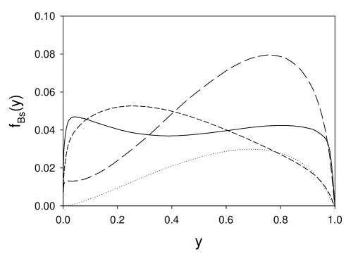
Figure 1: Bosonic structure functions in Yukawa theory, with a two-boson truncation ($f_{B+}$: solid; $f_{B-}$: long dash) and a one-boson truncation ($f_{B+}$: short dash; $f_{B-}$: dotted). The constituent masses had the values $m_{0}=-1.7\mu_{0}$, $m_{1}=\mu_{1}=15\mu_{0}$. The resolutions used in the Gauss–Legendre method are $K=20$ and $N=30$.

3 Feynman-gauge QED

We apply these same techniques to QED.[9] The Feynman-gauge Lagrangian is

$${\mathcal{L}} = \sum_{i=0}^{1}\left(-\frac{1}{4}(-1)^{i}F_{i}^{\mu\nu}F_{i,\mu\nu}+(-1)^{i}\bar{\psi_{i}}(i\gamma^{\mu}\partial_{\mu}-m_{i})\psi_{i}\right.$$ (18)

$$\left.+B_{i}\partial_{\mu}A_{i}^{\mu}+\frac{1}{2}B_{i}B_{i}\right)-e\bar{\psi}\gamma^{\mu}\psi A_{\mu},$$

where $A^{\mu}=\sum_{i=0}^{1}A^{\mu}_{i}$, $\psi=\sum_{i=0}^{1}\psi_{i}$, and $F_{i}^{\mu\nu}=\partial^{\mu}A_{i}^{\nu}-\partial_{\nu}A_{i}^{\mu}$. The nondynamical fermion fields $\psi_{i-}$ are constrained by

$$i[(-1)^{i}\partial_{-}\psi_{i-}-ie\sum_{k}A_{k-}\sum_{j}\psi_{j-}]$$

$$=-[(i\gamma^{0}\gamma^{\perp})((-1)^{i}\partial_{\perp}\psi_{i+}-ie\sum_{k}A_{k\perp}\sum_{j}\psi_{j+})-(-1)^{i}m\gamma^{0}\psi_{i+}].$$

For the null combination $\psi_{-}=\psi_{0-}+\psi_{1-}$, this becomes

$$i\partial_{-}\psi_{-}=-[(i\gamma^{0}\gamma^{\perp})\partial_{\perp}\psi_{+}-m\gamma^{0}\psi_{+}],$$ (20)

which is independent of $A$ and can therefore be solved without inverting a covariant derivative. We then obtain the Hamiltonian without antifermion terms as being

$$P^{-}=\sum_{i,s}\int d\underline{p}\frac{m_{i}^{2}+p_{\perp}^{2}}{p^{+}}(-1)^{i}b_{i,s}^{\dagger}(\underline{p})b_{i,s}(\underline{p})$$

$$+\sum_{l,\mu}\int d\underline{k}\frac{\mu_{l}^{2}+k_{\perp}^{2}}{k^{+}}(-1)^{l}\epsilon^{\mu}a_{l}^{\mu\dagger}(\underline{k})a_{l}^{\mu}(\underline{k})$$

$$+\sum_{i,j,l,s,\mu}\int d\underline{p}d\underline{q}\left\{\left[b_{i,s}^{\dagger}(\underline{p})b_{j,s}(\underline{q})V^{\mu}_{ij,2s}(\underline{p},\underline{q})\right.\right.$$

$$\left.\left.\rule{36.135pt}{0.0pt}+b_{i,s}^{\dagger}(\underline{p})b_{j,-s}(\underline{q})U^{\mu}_{ij,-2s}(\underline{p},\underline{q})\right]a_{l\mu}^{\dagger}(\underline{q}-\underline{p})+h.c.\right\}\,,$$

where $\epsilon^{\mu}=(-1,1,1,1)$. The vertex functions $U$ and $V$ are given in Ref. qed.

The dressed electron state, without pair contributions and truncated to one photon, is

$$|\psi\rangle=\sum_{i}z_{i}b_{i+}(\underline{P})|0\rangle+\sum_{s,\mu,i,l}\int d\underline{k}f^{\mu}_{ils}(\underline{k})b_{is}^{\dagger}(\underline{k})a^{\dagger}_{l\mu}(\underline{P}-\underline{k})|0\rangle,$$ (22)

with one-photon–one-electron wave functions

$$f^{\mu}_{il+}(\underline{k}) = \frac{\sum_{j}(-1)^{j}z_{j}P^{+}V_{ij+}^{\mu}(\underline{k},\underline{P})}{1-\frac{m_{i}^{2}+k_{\perp}^{2}}{x}-\frac{\mu_{l}^{2}+k_{\perp}^{2}}{1-x}},$$ (23)

$$f^{\mu}_{il-}(\underline{k}) = \frac{\sum_{j}(-1)^{j}z_{j}P^{+}U_{ij+}^{\mu}(\underline{k},\underline{P})}{1-\frac{m_{i}^{2}+k_{\perp}^{2}}{x}-\frac{\mu_{l}^{2}+k_{\perp}^{2}}{1-x}}.$$ (24)

Substitution into $P^{+}P^{-}|\psi\rangle=M^{2}|\psi\rangle$ yields

$$(M^{2}-m_{i}^{2})z_{i} = \frac{\alpha}{2\pi}\int\frac{dx}{x}dk_{\perp}^{2}\sum_{j,k,l}(-1)^{j+k+l}z_{j}$$ (26)

$$\times\frac{m_{k}^{2}+k_{\perp}^{2}-2m_{k}(m_{j}+m_{i})x+m_{j}m_{i}x^{2}}{M^{2}x(1-x)-m_{k}^{2}(1-x)-\mu_{l}^{2}x-k_{\perp}^{2}}.$$

This is the same form as in the one-boson Yukawa problem, with $g^{2}\rightarrow 2e^{2}$ and $I_{1}\rightarrow-2I_{1}$, and an analytic solution is again obtained. From this solution we can compute various quantities, including the anomalous magnetic moment.[9]

4 A correlator in ${\mathcal{N}}$=(2,2) SYM theory

Reduction of ${\mathcal{N}}$=1 SYM theory from four to two dimensions provides the action we need. In light-cone gauge ($A_{-}=0$) it is

$$S^{\rm LC}_{1+1}=\int dx^{+}dx^{-}{\rm tr}\Bigg{[}\partial_{+}X_{I}\partial_{-}X_{I}+i\theta^{T}_{R}\partial^{+}\theta_{R}+i\theta^{T}_{L}\partial^{-}\theta_{L}$$

$$+\frac{1}{2}(\partial_{-}A_{+})^{2}+gA_{+}J^{+}+\sqrt{2}g\theta^{T}_{L}\epsilon_{2}\beta_{I}[X_{I},\theta_{R}]+\frac{g^{2}}{4}[X_{I},X_{J}]^{2}\Bigg{]}.$$

Here the trace is over color indices, the $X_{I}$ are the scalar fields and the remnants of the transverse components of the four-dimensional gauge field $A_{\mu}$, the two-component spinors $\theta_{R}$ and $\theta_{L}$ are remnants of the right-moving and left-moving projections of the four-component spinor in the four-dimensional theory. We also define $J^{+}=i[X_{I},\partial_{-}X_{I}]+2\theta^{T}_{R}\theta_{R}$, $\beta_{1}\equiv\sigma_{1}$, $\beta_{2}\equiv\sigma_{3}$, and $\epsilon_{2}\equiv-i\sigma_{2}$.

The stress-energy correlation function for ${\mathcal{N}}$=(8,8) SYM theory can be calculated on the string-theory side:[12] $\langle T^{++}(x)T^{++}(0)\rangle=(N_{c}^{3/2}/g)x^{-5}$. We find numerically that this is almost true in ${\mathcal{N}}$=(2,2) SYM theory.[14]

To compute the correlator,[13] we fix the total momentum $P^{+}$, compute the Fourier transform, and express the transform in a spectral decomposed form

$$\tilde{F}(P^{+},x^{-}) = \frac{1}{2L}\langle T^{++}(P^{+},x^{+})T^{++}(-P^{+},0)\rangle$$

$$= \sum_{i}\frac{1}{2L}\langle 0|T^{++}(P^{+})|i\rangle e^{-iP_{i}^{-}x^{+}}\langle i|T^{++}(-P^{+},0)|0\rangle.$$

The position-space form is recovered by Fourier transforming with respect to the discrete momentum $P^{+}=K\pi/L$, where $K$ is the integer resolution and $L$ the length scale of DLCQ.[2]  This yields

$$F(x^{-},x^{+})=\sum_{i}\Big{|}\frac{L}{\pi}\langle 0|T^{++}(K)|i\rangle\Big{|}^{2}\left(\frac{x^{+}}{x^{-}}\right)^{2}\frac{M_{i}^{4}}{8\pi^{2}K^{3}}K_{4}(M_{i}\sqrt{2x^{+}x^{-}}).$$ (29)

We then continue to Euclidean space by taking $r=\sqrt{2x^{+}x^{-}}$ to be real. The matrix element $(L/\pi)\langle 0|T^{++}(K)|i\rangle$ is independent of $L$. Its form can be substituted directly to give an explicit expression for the two-point function.

The correlator behaves like $1/r^{4}$ at small $r$:

$$\left(\frac{x^{-}}{x^{+}}\right)^{2}F(x^{-},x^{+})=\frac{N_{c}^{2}(2n_{b}+n_{f})}{4\pi^{2}r^{4}}(1-1/K).$$ (30)

For arbitrary $r$, it can be obtained numerically by either computing the entire spectrum (for “small” matrices) or using Lanczos iterations (for large).[13]

In Fig. 2, we plot the log derivative of the scaled correlation function[14]

$$f\equiv\langle T^{++}(x)T^{++}(0)\rangle\left(\frac{x^{-}}{x^{+}}\right)^{2}\frac{4\pi^{2}r^{4}}{N_{c}^{2}(2n_{b}+n_{f})}.$$ (31)

Figure 2: The log derivative of the scaled correlation function $f$ defined in Eq. (31) of the text. The resolution $K$ ranges from 3 to 12. For even $K$, $f$ becomes constant at large $r$ and the derivative goes to zero.

At small $r$, the results for $f$ match the expected $(1-1/K)$ behavior. At large $r$ the behavior is different between odd and even $K$, but as $K$ increases, the differing behavior is pushed to larger $r$. For even $K$, there is exactly one massless state that contributes to the correlator, while there is no massless state for odd $K$. The lowest massive state dominates for odd $K$ at large $r$; however, this state becomes massless as $K\to\infty$. In the intermediate-$r$ region, the correlator behaves like $r^{-4.75}$, or almost $r^{-5}$. The size of this intermediate region increases as $K$ gets larger.

5 ${\mathcal{N}}$=(1,1) SYM theory at finite temperature

In this case, the Lagrangian is ${\mathcal{L}}={\rm Tr}\left(-\frac{1}{4}F_{\mu\nu}F^{\mu\nu}+i\bar{\Psi}\gamma_{\mu}D^{\mu}\Psi\right)$, with $F_{\mu\nu}=\partial_{\mu}A_{\nu}-\partial_{\nu}A_{\mu}+ig[A_{\mu},A_{\nu}]$ and $D_{\mu}=\partial_{\mu}+ig[A_{\mu}]$. The supercharge in light-cone gauge is $Q^{-}=2^{3/4}g\int dx^{-}\left(i[\phi,\partial_{-}\phi]+2\psi\psi\right)\partial_{-}^{-1}\psi$. From the discrete form we can compute the spectrum, which at large-$N_{c}$ represents a collection of noninteracting modes. With a sum over these modes, we can construct the free energy at finite temperature from the partition function[17, 15] $e^{-p_{0}/T}$.

The one-dimensional bosonic free energy is

$${\mathcal{F}}_{B}=\frac{VT}{\pi}\sum_{n=1}^{\infty}\int_{M_{n}}^{\infty}dp_{0}\frac{p_{0}}{\sqrt{p_{0}^{2}-M_{n}^{2}}}\ln\left(1-e^{-p_{0}/T}\right),$$ (32)

and the fermionic free energy is

$${\mathcal{F}}_{F}=-\frac{VT}{\pi}\sum_{n=1}^{\infty}\int_{M_{n}}^{\infty}dp_{0}\frac{p_{0}}{\sqrt{p_{0}^{2}-M_{n}^{2}}}\ln\left(1+e^{-p_{0}/T}\right).$$ (33)

The contributions from the $K-1$ massless states in each sector are

$${\mathcal{F}}^{0}_{B}=-\frac{(K-1)\pi}{6}VT^{2},\;\;{\mathcal{F}}^{0}_{F}=-\frac{(K-1)\pi}{12}VT^{2}.$$ (34)

The total free energy, with the logs expanded as sums and the $p_{0}$ integral already performed, is

$${\mathcal{F}}(T,V)=-\frac{(K-1)\pi}{4}VT^{2}-\frac{2VT}{\pi}\sum_{n=1}^{\infty}{\sum_{l=0}^{\infty}}M_{n}\frac{K_{1}\left((2l+1)\frac{M_{n}}{T}\right)}{(2l+1)}.$$ (35)

The sum over $l$ is well approximated by the first few terms. We can represent the sum over $n$ as an integral over a density of states: $\sum_{n}\rightarrow\int\rho(M)dM$ and approximate $\rho$ by a continuous function. The integral over $M$ can then be computed by standard numerical techniques. We obtain $\rho$ by a fit to the computed spectrum of the theory and find $\rho(M)\sim\exp(M/T_{\rm{H}})$, with $T_{H}\sim 0.845\sqrt{\pi/g^{2}N_{c}}$, the Hagedorn temperature.[18]  From the free energy we can compute various other thermodynamic functions up to this temperature.[15]

6 Future work

Given the success obtained to date, these techniques are well worth continued exploration. In Yukawa theory, we plan to consider the two-fermion sector, in order to study true bound states. For QED the next step will be inclusion of two-photon states in the calculation of the anomalous moment. For SYM theories, we are now able to reach much higher resolutions, by computing on clusters. This will permit continued reexamination of theories where previous calculations were hampered by low resolution, particularly in more dimensions. Earlier work on inclusion of fundamental matter[19] can be extended to three dimensions and modified to include finite-$N_{c}$ effects, such as baryons with a finite number of partons and the mixing of mesons and glueballs. For all of this work, the ultimate goal is, of course, the development of techniques sufficient to solve quantum chromodynmics.

References

• [1] P.A.M. Dirac, Rev. Mod. Phys. 21, 392 (1949).
• [2] H.-C. Pauli and S.J. Brodsky, Phys. Rev. D 32, 1993 (1985); 2001 (1985).
• [3] S.J. Brodsky, H.-C. Pauli, and S.S. Pinsky, Phys. Rep. 301, 299 (1997).
• [4] I. Montvay and G. Münster, Quantum Fields on a Lattice (Cambridge U. Press, New York, 1994); J. Smit, Introduction to Quantum Fields on a Lattice (Cambridge U. Press, New York, 2002).
• [5] W. Pauli and F. Villars, Rev. Mod. Phys. 21, 4334 (1949).
• [6] S.J. Brodsky, J.R. Hiller, and G. McCartor, Phys. Rev. D 58, 025005 (1998) [arXiv:hep-th/9802120]; 60, 054506 (1999); 64, 114023 (2001): Ann. Phys. 296, 406 (2002).
• [7] S.J. Brodsky, J.R. Hiller, and G. McCartor, Ann. Phys. 305, 266 (2003).
• [8] S.J. Brodsky, J.R. Hiller, and G. McCartor, in preparation.
• [9] S.J. Brodsky, V.A. Franke, J.R. Hiller, G. McCartor, S.A. Paston, and E.V. Prokhvatilov, arXiv:hep-ph/0406325.
• [10] O. Lunin and S. Pinsky, in New Directions in Quantum Chromodynamics, edited by C.-R. Ji and D.-P. Min, AIP Conf. Proc. No. 494 (AIP, Melville, NY, 1999), p. 140, [arXiv:hep-th/9910222].
• [11] F. Antonuccio, O. Lunin, and S. Pinsky, Phys. Rev. D 59, 085001 (1999); P. Haney, J.R. Hiller, O. Lunin, S. Pinsky, and U. Trittmann, Phys. Rev. D 62, 075002 (2000); J.R. Hiller, S. Pinsky, and U. Trittmann, Phys. Rev. D 64, 105027 (2001).
• [12] F. Antonuccio, A. Hashimoto, O. Lunin, and S. Pinsky, JHEP 9907, 029 (1999).
• [13] J.R. Hiller, O. Lunin, S. Pinsky, and U. Trittmann, Phys. Lett. B 482, 409 (2000); J.R. Hiller, S. Pinsky, and U. Trittmann, Phys. Rev. D 63, 105017 (2001).
• [14] M. Harada, J.R. Hiller, S. Pinsky, and N. Salwen, to appear in Phys. Rev. D, arXiv:hep-ph/0404123.
• [15] J.R. Hiller, Y. Proestos, S. Pinsky, and N. Salwen, arXiv:hep-th/0407076.
• [16] Y. Matsumura, N. Sakai, and T. Sakai, Phys. Rev. D 52, 2446 (1995).
• [17] S. Elser and A.C. Kalloniatis, Phys. Lett. B 375, 285 (1996).
• [18] R. Hagedorn, Nuovo Cimento Suppl. 3, 147 (1965); Nuovo Cimento 56A, 1027 (1968).
• [19] J.R. Hiller, S.S. Pinsky, and U. Trittmann, Nucl. Phys. B 661, 99 (2003); Phys. Rev. D 67, 115005 (2003).