Heavy Quarks on the Lattice

Abstract

Lattice quantum chromodynamics provides first principles calculations for hadrons containing heavy quarks — charm and bottom quarks. Their mass spectra, decay rates, and some hadronic matrix elements can be calculated on the lattice in a model independent manner. In this review, we introduce the effective theories that treat heavy quarks on the lattice. We summarize results on the heavy quarkonium spectrum, which verify the validity of the effective theory approach. We then discuss applications to $B$ physics, which is the main target of the lattice theory of heavy quarks. We review progress in lattice calculations of the $B$ meson decay constant, the $B$ parameter, semi-leptonic decay form factors, and other important quantities.

1 Introduction

Quantum chromodynamics (QCD) is the fundamental theory of the strong interaction. It is the SU(3) gauge field theory, which describes the interaction among quarks carrying three (R, G, and B) internal degrees of freedom, conveniently called “color.” Because of the non-Abelian nature of gauge symmetry, the gluon (the gauge field in QCD) interacts with itself, and as a result the strong coupling constant $\alpha_{s}$ becomes large as the momentum of the exchanged gluon decreases. Therefore, the calculation of low energy (approximately several hundred MeV) properties of hadrons, such as their masses and interactions, is a challenging problem that requires nonperturbative methods.

A regularized formulation of QCD on a four-dimensional hypercubic lattice, called lattice QCD Wilson:1974sk , enables us to calculate such hadron properties in the strong coupling regime. Because the interaction is highly nonlinear and the number of degrees of freedom is huge (proportional to the space-time volume), the lattice calculation is computationally so demanding that several dedicated supercomputers have been developed around the world. The application of lattice QCD covers a wide area including the light hadron mass spectrum, finite temperature phase transition, and weak-interaction matrix elements — as well as heavy quark physics, which is the subject of this article.

Among the six flavors of quarks in the Standard Model, charm ($c$), bottom ($b$), and top ($t$) quarks are heavy compared to the hadronic energy scale. The top quark decays very rapidly to a real $W$ boson and bottom quark, and its QCD interaction can be treated perturbatively. Therefore, we consider the physics of charm and bottom quarks.

The main motivation for charm and bottom quark physics is to study the flavor structure of the Standard Model including the mechanism that induces CP violation. Detailed study of the decays of charmed and bottom mesons provides pieces of information to precisely determine the Cabibbo-Kobayashi-Maskawa (CKM) matrix elements, which are fundamental parameters in the Standard Model. Furthermore, the loop effect of physics beyond the Standard Model may be probed through flavor-changing neutral current (FCNC) processes, such as $B^{0}$-$\bar{B}^{0}$ ($D^{0}$-$\bar{D}^{0}$) mixing or rare $B$ decays, which are suppressed in the Standard Model by the Glashow-Iliopuolos-Maiani (GIM) mechanism Glashow:gm . In such studies model-independent calculations of the hadronic matrix elements are crucial in order to precisely predict the Standard Model contributions.

One example is the rate (or frequency) of the neutral $B$ meson mixing, which is induced by $\Delta B=2$ box diagrams. Because of the GIM mechanism, the dominant contribution comes from the diagram involving the top quark, which is proportional to the CKM matrix element $|V_{td}|$ squared. At the $B$ meson energy scale, this interaction is effectively described by a local operator $O^{\Delta B=2}=\bar{b}\gamma_{\mu}(1-\gamma_{5})q\,\bar{b}\gamma_{\mu}(1-\gamma_{5})q$, and its rate is proportional to a matrix element $\langle\bar{B}|O^{\Delta B=2}|B\rangle$, which is parametrized by the $B$ meson decay constant $f_{B}$ and the $B$-parameter $B_{B}$. This matrix element represents the probability of finding the heavy quark and the light anti-quark at the same spatial point in the $B$ meson to annihilate it and to create a $\bar{B}$ meson from that point. This is a problem of bound state formation in QCD, which is non-perturbative. The lattice calculation offers the best tool to solve such problems, but one needs a special treatment of heavy quark fields on the lattice, since the Compton wavelength of the heavy quark, $\sim 1/m_{Q}$, could be smaller than the typical lattice spacing $a$.

The typical energy or momentum scale that governs the dynamics of quarks and gluons inside the usual light hadrons is the QCD scale $\Lambda_{\mathrm{QCD}}$, which characterizes the energy scale where the QCD coupling $\alpha_{s}$ becomes large. Because the heavy quark introduces a new energy scale to the system, the QCD dynamics inside heavy hadrons is quite different from that of light hadrons.

Figure 1: Typical momentum scales in the heavy-light (left) and heavy-heavy (right) mesons.

In the heavy-light meson, which is a bound state composed of a heavy quark $Q$ and light degrees of freedom (a light anti-quark $\bar{q}$ and gluons $g$), the motion of the heavy quark of mass $m_{Q}$ is hardly affected by the light degrees of freedom with a typical momentum $\Lambda_{\mathrm{QCD}}$, if $m_{Q}\gg\Lambda_{\mathrm{QCD}}$. Thus, the heavy quark stays almost at rest at the center of the bound state, surrounded by the light degrees of freedom, as shown in the left panel of Figure 1. The motion of the heavy quark is suppressed by $\Lambda_{\mathrm{QCD}}/m_{Q}$. This system is described by the Heavy Quark Effective Theory (HQET) Eichten:1989zv ; Georgi:1990um ; Grinstein:1990mj , which is discussed in Section 2.

The dynamics of quarkonium, which is a bound state of $Q$ and $\bar{Q}$, is governed by different energy scales. In the classical picture, the nonrelativistic kinetic energy $\langle p^{2}\rangle/2m_{Q}$ and the potential energy $-\frac{4}{3}\alpha_{s}\langle\frac{1}{r}\rangle$ have to be balanced, and the heavy quarks move around each other, in contrast to the heavy-light dynamics, as depicted in Figure 1 (right panel). $\langle p\rangle$ and $\langle\frac{1}{r}\rangle$ denote the typical size of the relative spatial momentum and distance between the two heavy quarks, respectively. The uncertainty relation $\langle p\rangle\sim\langle 1/r\rangle$ implies $\langle p\rangle\sim\alpha_{s}m_{Q}$, which means that the typical velocity $v\sim\langle p\rangle/m_{Q}$ is of the order of the strong coupling constant $\alpha_{s}$. Thus, there are three momentum scales in the heavy quarkonia: heavy quark mass $m_{Q}$, typical spatial momentum $\langle p\rangle\simeq m_{Q}v$, and typical binding energy $\langle p^{2}\rangle/m_{Q}\simeq m_{Q}v^{2}$. It is possible to construcnt an effective theory that explicitly separates these energy scales. This is known as non-relativistic QCD (NRQCD) Caswell:1985ui ; Thacker:1990bm ; Lepage:1992tx .

A number of lattice simulations for heavy quarks have been performed with or without these effective theories. For the heavy-light mesons, the simplest and best known application is the calculation of the $B$ meson decay constant. Other more complicated quantities include the $B$-parameters and the semi-leptonic decay form factors. These quantities are not known from experimental data, and are necessary inputs to determine the CKM matrix elements. For the heavy-heavy mesons, on the other hand, the mass spectrum of $c\bar{c}$ and $b\bar{b}$ quarkonia is experimentally very well known, and thus provides a benchmark by which to test the validity of the lattice calculations.

Until recently, because of the lack of computer power, most lattice simulations have been done in the quenched approximation, in which the effect of quark-antiquark pair creation (and annihilation) in the vacuum is neglected. This approach could introduce uncontrolled systematic uncertainty, and hence the results should not be taken as a model independent prediction. However, the full QCD simulation without such an approximation has become realistic recently. We review some results from such calculations.

This article is organized as follows. In Section 2 we introduce the effective theories used for heavy-light and heavy-heavy systems, and discuss their lattice formulations. Matching of the effective theory onto the continuum QCD is one of the key issues. Some results for quarkonia mass spectrum and decays are discussed in Section 3. Model independent calculation of the matrix elements required in $B$ physics phenomenology is the main motivation for the study of heavy quark on the lattice. We review the current status in Section 4. Finally, the prospects for future lattice calculations are discussed in Section 5.

We do not discuss the determination of the bottom quark mass using the lattice results for quarkoinum because it was well covered in a recent review by El-Khadra & Luke El-Khadra:2002wp . Reviews presented at recent lattice conferences Bernard:2000ki ; Ryan:2001ej ; Yamada:2002wh ; Kronfeld:2003sd and in other review articles Flynn:1997ca ; Kronfeld:2003sd are also useful sources of information. For textbooks on lattice gauge theory, see for example Montvay:cy ; Smit:ug .

2 HQET and NRQCD

The lattice spacing $a$ in today’s typical lattice simulations is about 0.1–0.2 fm. The available physical volume is then $V\simeq(2\mathrm{~{}fm})^{3}$ for the typical lattice size $L/a=$ 16–24, which is numerically feasible. Because the Compton wavelength of charm and bottom quarks ($1/m_{c}\simeq 0.13\mathrm{~{}fm}$ and $1/m_{b}\simeq 0.04\mathrm{~{}fm}$, respectively) are similar to or even smaller than the lattice spacing, discretization errors would seem to be out of control. Naively, the discretization error grows as $(am_{Q})^{n}$, and the power $n$ is 2 for the $O(a)$-improved lattice fermion actions, such as the $O(a)$-improved Wilson fermion Sheikholeslami:1985ij .

However, the non-perturbative dynamics of QCD becomes important only in the low energy ($\sim\Lambda_{\mathrm{QCD}}$) regime. Therefore, if one can formulate the theory such that the energy scale of order $m_{Q}$ is explicitly separated from the low energy degrees of freedom, it would suffice to treat only the low energy part in the lattice simulation; the high energy part can be reliably treated in perturbation theory. Theoretically, such separation of different energy scales can be formulated in terms of the Operator Product Expansion (OPE) Wilson:zs . Its well-known application is in deep inelastic scattering, for which the large energy scale comes the energy of collisions. Lagrangian-based formulations are more transparent in many applications, and for the heavy-light and heavy-heavy hadrons dedicated formulations have been developed: Heavy Quark Effective Theory (HQET) for the heavy-light and nonrelativistic QCD (NRQCD) for the heavy-heavy hadrons.

2.1 Continuum HQET and NRQCD

Let us consider a heavy hadron in its rest frame. The momentum of the heavy quark inside the heavy hadron can be written as $p_{Q}^{\mu}=(m_{Q}+k^{0},\mbox{\boldmath$k$})$ by separating the heavy quark mass $m_{Q}$ from other, smaller momentum. From the heavy quark field $q$ one may extract the trivial dependence on the heavy quark mass as $q=e^{-im_{Q}t}\left(\begin{array}[c]{c}Q\\ X\end{array}\right)$, where the four-component spinor is divided into two two-component spinors $Q$ and $X$. Then, the Dirac equation $(i\gamma^{\mu}D_{\mu}-m_{Q})q=0$ with the Dirac representation of the $\gamma$ matrices can be separated into two parts:

$$iD_{0}\,Q = i\mbox{\boldmath$\sigma$}\cdot\mbox{\boldmath$D$}\,X,$$ (1)

$$(2m_{Q}+iD_{0})\,X = i\mbox{\boldmath$\sigma$}\cdot\mbox{\boldmath$D$}\,Q,$$ (2)

where $\sigma^{i}$ are the Pauli matrices. The second equation shows that the lower component $X$ is smaller than the upper component $Q$ by a factor $2m_{Q}$. If we can neglect the small time-dependence of $X$, $iD_{0}X$ in Equation 2, and substitute $X=i\mbox{\boldmath$\sigma$}\cdot\mbox{\boldmath$D$}/2m_{Q}Q$ into Equation 1, we arrive at the non-relativistic Shrödinger equation plus the Pauli term,

$$iD_{0}\,Q=-\left[\frac{\mbox{\boldmath$D$}^{2}}{2m_{Q}}+\frac{\mbox{\boldmath$\sigma$}\cdot g\mbox{\boldmath$B$}}{2m_{Q}}\right]Q,$$ (3)

where $g$ is the QCD coupling constant and $B^{i}=\frac{1}{2}\epsilon^{ijk}F^{jk}$ is the magnetic part of the field-strength tensor of QCD. In Lagrangian form we may write this as

$$\mathcal{L}_{\mathrm{heavy}} = Q^{\dagger}\left[iD_{0}+\frac{\mbox{\boldmath$D$}^{2}}{2m_{Q}}+\frac{\mbox{\boldmath$\sigma$}\cdot g\mbox{\boldmath$B$}}{2m_{Q}}+\frac{\mbox{\boldmath$D$}\cdot g\mbox{\boldmath$E$}-g\mbox{\boldmath$E$}\cdot\mbox{\boldmath$D$}}{8m_{Q}^{2}}\right.$$ (4)

$$\left.+\frac{\mbox{\boldmath$\sigma$}\cdot(i\mbox{\boldmath$D$}\times g\mbox{\boldmath$E$}-g\mbox{\boldmath$E$}\times i\mbox{\boldmath$D$})}{8m_{Q}^{2}}+\frac{(\mbox{\boldmath$D$}^{2})^{2}}{8m_{Q}^{3}}+\cdots\right]Q,$$

recovering some of the higher order contributions. The ellipses represent neglected higher order terms.

In the heavy-light hadron, the light degrees of freedom (light quarks and gluons) have momenta of order $\Lambda_{\mathrm{QCD}}$. Exchange of spatial momenta with the heavy quark occurs through the $1/m_{Q}$ and higher order terms in Equation 4. Thus, the motion of the heavy quark is suppressed by powers of $\Lambda_{\mathrm{QCD}}/m_{Q}$. In HQET Eichten:1989zv ; Georgi:1990um ; Grinstein:1990mj one treats the Lagrangian equation (Equation 4) as a systematic expansion in $1/m_{Q}$. At leading order, only the first term $Q^{\dagger}iD_{0}Q$ remains, which represents a non-moving heavy quark acting only as a static color source. This is often called the static approximation. The higher order terms can be included by operator insertions, that is, by expanding $\exp(i\int d^{4}x\mathcal{L}_{heavy})$ in terms of $1/m_{Q}$. In the lattice simulations, it is more convenient to include the higher order terms as a part of the heavy quark propagator.

In the heavy-heavy hadron, on the other hand, the momentum of the heavy (anti-)quark is determined by the balance between the potential energy and kinetic energy, as already mentioned in Section 1. Specifically, in order to satisfy Equation 3, $\langle iD_{0}Q\rangle\sim\langle\mbox{\boldmath$D$}^{2}/2m_{Q}Q\rangle$. Because the heavy quark potential is well described by the Coulomb form $-C_{F}\alpha_{s}/r$, this implies

$$\langle\frac{\alpha_{s}}{r}\rangle\sim\langle\alpha_{s}p\rangle\sim\frac{\langle p^{2}\rangle}{m_{Q}}.$$ (5)

Then, the typical momentum is of the order $m_{Q}\alpha_{s}$, or the typical velocity $v=\langle p\rangle/m_{Q}$ is of order $\alpha_{s}$. The separation of the energy scales is provided by the velocity $v$: (heavy quark mass $m_{Q}$) $\gg$ (momentum $m_{Q}v$) $\gg$ (binding energy $m_{Q}v^{2}$).

In NRQCD Caswell:1985ui ; Thacker:1990bm ; Lepage:1992tx the counting of terms in the Lagrangian equation (Equation 4) is done by the power of $v$. Each operator has a different power counting: $Q\sim(m_{Q}v)^{3/2}$, $\mbox{\boldmath$D$}\sim m_{Q}v$, $D_{0}\sim m_{Q}v^{2}$, $g\mbox{\boldmath$E$}\sim m_{Q}^{2}v^{3}$, and $g\mbox{\boldmath$B$}\sim m_{Q}^{2}v^{4}$. As a result, the leading terms in Equation 4 are $Q^{\dagger}iD_{0}Q$ and $Q^{\dagger}(-\mbox{\boldmath$D$}^{2}/2m_{Q})\,Q$; the other terms are suppressed by a relative power $v^{2}$. Higher order terms can also be included in a systematic manner.

The QCD coupling constant $\alpha_{s}$ depends on the energy scale, according to the renormalization group running. It should be evaluated at the momentum of the exchanged gluons, which in this case is the momentum scale of $m_{Q}v\sim m_{Q}\alpha_{s}$. By solving $v\sim\alpha_{s}(m_{Q}v)$ self-consistently, the typical velocity squared is estimated to be $v^{2}\sim$ 0.3 for charmonium ($c\bar{c}$) and 0.1 for bottomonium ($b\bar{b}$). Expansion in $v^{2}$ is therefore very effective for $b\bar{b}$ but marginal for $c\bar{c}$.

2.2 Lattice HQET and NRQCD

Once the effective theories are introduced, the length scale to be treated on the lattice is not $1/m_{Q}$, but $1/\Lambda_{\mathrm{QCD}}$ for heavy-light or $1/m_{Q}v$ for heavy-heavy systems. These are long enough to be approximated by a lattice of $a\sim$ 0.1–0.2 fm. A rough sketch of the relevant length scales is shown in Figure 1.

Discretization of the Lagrangian equation (Equation 4) is straightforward. First, one must perform the Wick rotation $x^{0}=ix_{4}$ to move on to the Euclidean space-time. Then, the covariant derivative $D_{\mu}$ is replaced by a finite difference

$$\Delta^{(+)}_{\mu}Q(x)\equiv U_{\mu}(x)Q(x+\hat{\mu})-Q(x),$$ (6)

where $x+\hat{\mu}$ denotes a lattice point next to $x$ in the $\mu$-direction. $U_{\mu}(x)$ is the link variable, which represents the gauge field on the lattice: the relation to the continuum vector potential $A_{\mu}(x)$ is approximately given by $U_{\mu}(x)=\exp[iagA_{\mu}(x)]$. The discretized derivative, Equation 6, is constructed such that it is covariant under the SU(3) gauge transformation. One can also define

$$\Delta^{(-)}_{\mu}Q(x)\equiv Q(x)-U^{\dagger}_{\mu}(x-\hat{\mu})Q(x-\hat{\mu}),$$ (7)

$\Delta^{(\pm)}_{\mu}=(\Delta^{(+)}+\Delta^{(-)})/2$, and the lattice Laplacian $\Delta^{(2)}\equiv\sum_{i}\Delta_{i}^{(+)}\Delta_{i}^{(-)}$.

One explicit form of the lattice action is

$$S=\sum_{t,\mbox{\boldmath$x$}}Q^{\dagger}(t,\mbox{\boldmath$x$})[Q(t,\mbox{\boldmath$x$})-K_{t}Q(t-1,\mbox{\boldmath$x$})],$$ (8)

where $t=x_{4}$. The operator $K_{t}$ is a kernel of time-evolution:

$$K_{t}=\left(1-\frac{aH_{0}}{2n}\right)_{t}^{n}\left(1-\frac{a\delta H}{2}\right)_{t}U_{4,t-1}^{\dagger}\left(1-\frac{a\delta H}{2}\right)_{t-1}\left(1-\frac{aH_{0}}{2n}\right)_{t-1}^{n}.$$ (9)

Here subscripts represent the time slice at which Hamiltonian operators such as $(1-aH_{0}/2n)$ act, and an integer $n$ is introduced to suppress instability that appears in the evolution equation owing to unphysical momentum modes Thacker:1990bm ; Lepage:1992tx . The leading order Hamiltonian $H_{0}$ is given by

$$H_{0}=-\frac{\Delta^{(2)}}{2m_{Q}},$$ (10)

and the higher order terms are

$$\delta H = -\frac{\mbox{\boldmath$\sigma$}\cdot g\mbox{\boldmath$B$}}{2m_{Q}}-\frac{\mbox{\boldmath$\Delta$}^{(\pm)}\cdot g\mbox{\boldmath$E$}-g\mbox{\boldmath$E$}\cdot\mbox{\boldmath$\Delta$}^{(\pm)}}{8m_{Q}^{2}}-\frac{\mbox{\boldmath$\sigma$}\cdot(\mbox{\boldmath$\Delta$}^{(\pm)}\times g\mbox{\boldmath$E$}-g\mbox{\boldmath$E$}\times\mbox{\boldmath$\Delta$}^{(\pm)})}{8m_{Q}^{2}}$$ (11)

$$-\frac{(\Delta^{(2)})^{2}}{8m_{Q}^{3}}+\cdots.$$

The field strength tensors $B$ and $E$ are made from link variables connected on a plaquette. Details of their construction are given, for instance, in Reference Lepage:1992tx . One can also define other heavy quark actions, which are equivalent to Equation 8 up to discretization effects.

Because the propagation of the heavy quark is simply expressed by the time-evolution kernel, Equation 9, numerical calculation of the heavy quark propagator is much faster than calculation of the light quark propagator, which requires some iterative solver, such as the conjugate gradient method.

As in the continuum case, the difference between HQET and NRQCD is in the underlying dynamics. We can use the same lattice action, but the size of the contribution from each term in the Lagrangian differs between heavy-light and heavy-heavy hadrons. In other words, at a given accuracy (say $\Lambda_{\mathrm{QCD}}/m_{Q}$ in the heavy-light, or $v^{2}$ in the heavy-heavy), the terms to be included in the calculation are different.

To recover the original four-component Dirac spinor $\psi_{h}$ from the two-component fields, one must apply the Foldy-Wouthuysen-Tani (FWT) transformation

$$\psi_{h}=\left[1-\frac{\mbox{\boldmath$\gamma$}\cdot\Delta^{(\pm)}}{2m_{Q}}+\frac{\Delta^{(2)}}{8m_{Q}^{2}}+\frac{\mbox{\boldmath$\Sigma$}\cdot g\mbox{\boldmath$B$}}{8m_{Q}^{2}}-\frac{i\gamma_{4}\mbox{\boldmath$\gamma$}\cdot g\mbox{\boldmath$E$}}{4m_{Q}^{2}}+\cdots\right]\left(\begin{array}[c]{c}Q\\ 0\end{array}\right),$$ (12)

with $\Sigma^{j}=\mathrm{diag}\{\sigma^{j},\sigma^{j}\}$. It is necessary when we construct operators that involve both heavy and light quark fields, such as the heavy-light axial-vector current $A_{\mu}=\bar{\psi}_{h}\gamma_{5}\gamma_{\mu}\psi_{l}$.

In the language of the functional integral to define the quantum field theory, the FWT transformation is nothing but a change of variables, and the physics described by the theories before and after the transformation is the same up to neglected higher order terms in Equation 12. There is a class of possible such transformations, but the choice in Equation 12 is special because it removes the lower components from the theory. This suggests that there are other effective theories for which the FWT transformation is partially applied. Such a formulation is known as the Fermilab action El-Khadra:1996mp ; Kronfeld:2000ck . It uses the usual four-component spinors on the lattice, and the higher spatial derivatives are introduced according to the order counting of HQET or NRQCD. This formulation is useful, because at the leading order (of $1/m_{Q}$ or $v^{2}$) the action can be taken to be the same as that of light quark actions, i.e. the Wilson fermion with or without the $O(a)$-improvement. Therefore, this formalism covers entire mass regions (from light to heavy) with a single fermion action, although the achievable accuracy varies depending on the quark mass. In the heavy quark regime the accuracy is estimated in terms of the HQET or NRQCD counting rule. The discretization effect can also be estimated by interpreting the lattice effective action with the Symanzik effective theory Kronfeld:2000ck . To correctly incorporate the higher order corrections one must introduce higher derivative terms to the action just as in the NRQCD action. An equivalent formulation, but without the FWT transformation, was proposed later in a different context Aoki:2001ra .

2.3 Renormalization and continuum limit of the effective theories

Although the HQET and NRQCD capture the physical picture of the heavy quark inside the heavy hadrons, the resulting field theory is a non-renormalizable effective theory. This means that an infinite number of terms are needed in order to eliminate ultraviolet divergences that appear in quantum loop calculations of the theory. In fact the Lagrangian equation (Equation 4) contains infinitely many terms at higher orders, and to renormalize them one needs an infinite number of renormalization conditions, i.e. input parameters. In practice, one is only interested in finite orders of $1/m_{Q}$ (or $v^{2}$) and truncates the Lagrangian at that order. Then, the number of renormalization conditions is finite and the calculation is feasible. This is how these effective theories work: at a certain order of the systematic expansion the number of parameters is still finite, and thus the predictive power remains.

On the lattice with a finite lattice spacing no divergence appears, but we still need input parameters. The coefficients in front of the terms in Equation 11 are correct only at tree level; if we include the quantum effects, they become renormalized. These input parameters are provided by calculating some physical amplitudes in the full relativistic theory. The coefficients are then determined such that the effective theory gives the same physical amplitude at a given order of $1/m_{Q}$ (or $v^{2}$). This procedure is called matching, and it is usually done in perturbation theory (perturbative matching).

At leading order the necessary terms are $Q^{\dagger}Q$, $Q^{\dagger}D_{0}Q$ and $Q^{\dagger}\mbox{\boldmath$D$}^{2}Q$. Their renormalization corresponds to the energy shift, wave function renormalization, and mass renormalization, respectively. The perturbative matching of these parameters onto continuum full theory was calculated for several specific definitions of lattice NRQCD actions Davies:1991py ; Morningstar:1993de ; Morningstar:1994qe ; Ishikawa:1999xu and for the Fermilab action Mertens:1997wx , although the complete calculation of higher order terms, especially the term $\mbox{\boldmath$\sigma$}\cdot\mbox{\boldmath$B$}$, is still to be done.

Similarly, the operators to be measured on the lattice must be matched onto the continuum full theory. For example, the heavy-light axial-vector current $A_{\mu}=\bar{\psi}_{h}\gamma_{5}\gamma_{\mu}\psi_{l}$, which is related to the $B$ meson leptonic decay constant, is renormalized as

$$\mathcal{A}_{4}=Z_{A}\left[\bar{\psi}_{h}\gamma_{5}\gamma_{4}\psi_{l}-\frac{c_{A}^{(1)}}{2m_{Q}}\bar{\psi}_{h}\gamma_{5}\gamma_{4}\mbox{\boldmath$\gamma$}\cdot\mbox{\boldmath$\Delta$}^{(\pm)}\psi_{l}+\frac{c_{A}^{(2)}}{2m_{Q}}\bar{\psi}_{h}\gamma_{5}\gamma_{4}\mbox{\boldmath$\gamma$}\cdot\overleftarrow{\mbox{\boldmath$\Delta$}}^{(\pm)}\psi_{l}\right],$$ (13)

for the continuum heavy-light axial-vector current $\mathcal{A}_{\mu}$ defined, for instance, using the $\overline{\mathrm{MS}}$ scheme. The matching parameters $Z_{A}$, $c_{A}^{(1)}$, and $c_{A}^{(2)}$ are calculated at the one-loop level of perturbation theory. In the static limit ($m_{Q}\rightarrow\infty$), the perturbative calculation of $Z_{A}$ was carried out for both the Wilson Boucaud:1989ga ; Eichten:1989kb ; Boucaud:1992nf and the $O(a)$-improved Wilson Borrelli:1992fy ; Hernandez:1992su fermions for the light quark, and even a non-perturbative calculation has been done recently Heitger:2003xg . One-loop calculations are also available for the NRQCD Davies:ec ; Morningstar:1997ep ; Morningstar:1998yx ; Ishikawa:1999xu and for the Fermilab Harada:2001fi lattice actions. The matching of the four-quark operator $O_{L}=\bar{\psi}_{h}\gamma_{5}(1-\gamma_{\mu})\psi_{l}\bar{\psi}_{h}\gamma_{5}(1-\gamma_{\mu})\psi_{l}$, which is needed for the the $B^{0}$-$\bar{B}^{0}$ mixing matrix elements, has also been calculated Flynn:1990qz ; Borrelli:1992fy ; DiPierro:1998ty ; Gimenez:1998mw ; Ishikawa:1998rv ; Hashimoto:2000eh .

The continuum limit of the lattice HQET/NRQCD is not trivial. Beyond the static approximation, the lattice action contains higher dimensional operators that induce power divergent terms such as $1/(am_{Q})^{n}$ in the radiative corrections. Because the divergences are unphysical and must be subtracted (or renormalized), the perturbative matching becomes less accurate as $a\rightarrow 0$, even though the physical picture of the $\Lambda_{\mathrm{QCD}}/m_{Q}$ (or $v^{2}$) expansion does not change. Therefore, the lattice calculation is practically restricted to relatively large lattice spacings, such that $am_{Q}\gtrsim 1$ is maintained. This means that the continuum limit $a\rightarrow 0$ cannot be reached within the effective theories beyond the leading order (static limit), and one must check the stability of the results in a limited region of lattice spacings to keep $am_{Q}\gtrsim 1$. For the Fermilab action El-Khadra:1996mp , on the other hand, the continuum limit can smoothly be reached, because it is reduced to the Wilson-like fermions as $am_{Q}\rightarrow 0$.

In the dimensional regularization adopted in the continuum perturbation theory, the problem of power divergences in the OPE appears as the renormalon ambiguity Martinelli:1996pk ; that is, the lowest order Wilson coefficient contains an ambiguity of order $\Lambda_{\mathrm{QCD}}/m_{Q}$ due to the poor convergence behavior of the perturbative expansion. The renormalon ambiguity cancels with the higher order matrix element of the same order ($\Lambda_{\mathrm{QCD}}/m_{Q}$), and the physical quantity to be computed is free from the ambiguity. In the theory with an explicit cutoff, such as lattice gauge theory, the problem becomes the difficulty of subtracting unphysical power divergences using the perturbative expansion, as discussed above. In practice, the perturbative expansion converges well as far as one keeps $am_{Q}\gtrsim 1$, but higher order perturbative calculations are needed to obtain better control of systematic errors Bernard:2000ki ; Kronfeld:2003sd .

One can avoid the whole problem by performing the matching calculation non-perturbatively, as recently proposed by the ALPHA collaboration Heitger:2003nj . The matching of lattice HQET onto the relativistic action is feasible on a lattice of physically small volume, $L\simeq$ 0.2 fm, because one can work with a small lattice spacing for which the relativistic action can be safely used. The matching of HQET on larger volumes is then performed by comparing the lattices of size $L$ and $2L$ recursively. At present, the method is applied to the leading-order HQET (static limit), but if the matching could be done in a similar manner for higher dimensional operators, it would provide a breakthrough to go beyond perturbative matching.

2.4 Relativistic lattice actions used for heavy quarks

In the usual lattice fermion actions, the quark mass is included as a perturbation to the massless limit. Because the theory is renormalizable, the number of relevant operators is limited and the transition toward the continuum limit is straightforward.

However, in practical simulations with present computer resources, the lattice spacing $a$ is not always small enough to satisfy $am_{Q}\ll 1$ for the charm quark, and it is absolutely too large for the bottom quark. The discretization error starts from $O(am_{Q})$ for the unimproved Wilson fermion, or from $O[(am_{Q})^{2}]$ for the $O(a)$-improved actions.

One can see how the discretization errors behave by taking the energy-momentum dispersion relation as an example. The non-relativistic effective Hamiltonian of the “relativistic” lattice fermion can be written as

$$\mathcal{H}_{\mathrm{heavy}}=Q^{\dagger}\left[m_{1}-\frac{\mbox{\boldmath$D$}^{2}}{2m_{2}}+\cdots\right]Q,$$ (14)

where the rest mass $m_{1}$ and the kinetic mass $m_{2}$ can be different if the Lorentz invariance is lost owing to the discretization error. At tree level they become

$$m_{1}a = \ln(1+m_{0}a),$$ (15)

$$\frac{1}{m_{2}a} = \frac{2}{m_{0}a(2+m_{0}a)}+\frac{1}{1+m_{0}a},$$ (16)

for the $O(a)$-improved and -unimproved Wilson fermions, respectively. The term $m_{0}$ denotes the quark mass appearing in the relativistic lattice action. Then the problem appears as a violation of the relation $m_{0}=m_{1}=m_{2}$ of order $(am_{Q})^{2}$.

One way to avoid the problem of this large $am_{Q}$ error is to reinterpret the lattice action using HQET as done in the Fermilab formulation El-Khadra:1996mp . But, if one does not employ this reinterpretation, one must restrict oneself to the region where $am_{Q}$ is small enough that the remaining errors of order $(am_{Q})^{2}$ and higher are under control. This is possible for the charm quark if one takes the lattice cutoff much higher than 2 GeV and eliminates the leading error $(am_{Q})^{2}$ by an extrapolation to the continuum limit, although it is numerically rather demanding. Such analysis has been done only recently for the charm quark mass Rolf:2002gu and for the $D_{s}$ meson decay constant Juttner:2003ns in the quenched approximation.

To reach the bottom quark mass one must rely on an extrapolation in the heavy quark mass. It can be done by using the heavy quark scaling law, e.g. for heavy enough quark masses the heavy-light meson decay constant $f_{P}$ behaves as $1/\sqrt{M_{P}}$ up to power corrections. This method requires a careful analysis because the discretization error of order $(am_{Q})^{2}$ grows as $m_{Q}$ becomes larger, and this growth could even be amplified by the extrapolation, producing uncontrolled systematic errors. An extrapolation to the continuum limit $a\to 0$ must be done before the heavy quark extrapolation to reduce such a problem. A combined fit with the result in the static limit may be used to stabilize the extrapolation.

Because the large energy scale of order $m_{Q}$ flows only in the temporal direction in the rest frame, the discretization error appears from the temporal derivative of the lattice action. It is therefore possible to avoid the large discretization error by taking a temporal lattice spacing $a_{t}$ much smaller than $1/m_{Q}$ while keeping the spatial lattice spacing $a_{s}$. This is called the anisotropic lattice action Alford:1996nx . Although the radiative correction could reintroduce large $\alpha_{s}m_{Q}a_{s}$ contributions, in wihch case the virtue of the anisotropy is lost Harada:2001ei ; Aoki:2001ra , it is also possible to construct lattice actions free from this problem Hashimoto:2003fs .

3 Quarkonia

Since the discovery of $J/\psi$, experimental studies of heavy quarkonia have produced enormously rich and precise data for their mass spectra and decay rates. Theoretically, the quark potential model description has been successful in explaining their properties, indicating that heavy quarkonium is a non-relativistic bound state. Therefore, the study of quarkonia gives a firm testing ground for lattice QCD, and the results may also be used to calibrate the basic parameter of the calculation, the lattice spacing $a$. Furthermore, the lattice QCD will be useful for studying the properties of non-standard states, such as $q\bar{q}g$ hybrids and $q\bar{q}q\bar{q}$ multi-quark states, which may depend on the details of non-perturbative QCD dynamics.

3.1 Mass spectrum

Heavy quarkonium is a system for which one of the most accurate calculations can be done on the lattice. Indeed, Davies et al. demonstrated that the mass spectrum can be precisely calculated using lattice NRQCD Davies:1994mp ; Davies:1995db ; Davies:1997mg ; Davies:1998im . They used the lattice NRQCD action including the entire $O(v^{4})$ terms as given in Equations 10 and 11. The leading discretization errors are eliminated by adding the $O(a^{2})$ improvement terms. The bottomonium spectrum obtained on the lattice with $1/a\simeq$ 2.4 GeV is shown in Figure 2 Davies:1997mg ; Davies:1998im . The masses of low-lying radial and orbitally excited states are precisely computed in both quenched ($N_{f}=0$) and unquenched ($N_{f}=2$) QCD. It is remarkable that the 1S-2S and 1S-1P splittings become more consistent with the experimental value if dynamical quarks are introduced.

Figure 2: Bottomonium spectrum from Reference Davies:1997mg . The spin dependent splittings of the 1P states are shown separately in the right panel. Dashed lines indicate the experimental value. The lattice data are for $N_{f}=0$ (filled circles) and $N_{f}=2$ (open circles).

With the NRQCD formulation one can investigate the effect of each term included in the action by comparing the results with and without that contribution. Furthermore, because the bottomonium system is mostly sensitive to short distance physics, our experience from quark models and perturbation theory can be used to estimate the systematic uncertainty due to truncated higher order terms in $v^{2}$ and in $a$.

In the non-relativistic expansion the leading terms that are not included in the action employed by Davies et al. are those of $O(v^{6})$. Because the typical $v^{2}$ is about 0.1 for the bottomonium system, the relative error to the leading terms ($\sim v^{2}$) is naively $O(v^{4})\sim$ 1%. An estimate using the quark potential model suggests even smaller error Lepage:1991ui . The leading discretization errors are the radiative correction to the $O(a^{2})$ improvement term and the $O(a^{4})$ corrections. These are $O(\alpha_{s}(\pi/a)a^{2}p^{2})$ and $O(a^{4}p^{4})$, respectively, for typical spatial momentum $p=m_{Q}v$. For the lattice spacings between 0.05 fm and 0.15 fm the size of their corrections is estimated to be at most a few percent, and lattice data at three lattice spacings support such small discretization effects Davies:1998im .

For the spin-dependent splittings, the relative error is an order of magnitude larger because the leading contribution itself is $O(v^{4})$. Indeed, Manke et al. studied the effect of the tree-level $O(v^{6})$ corrections in quenched NRQCD and found that the spin-dependent splittings are affected by 10%–20% when $O(v^{6})$ terms are added to the action, whereas the spin-averaged splittings are essentially unaltered, supporting the above naive expectation Manke:1997gt .

As shown in Figure 2 the mass spectrum significantly deviates from experiment unless the effect of dynamical quarks is included. The sea quark effects have also been studied Eicker:1998vx ; Manke:2000dg and found to be sizable. The recent calculation by the HPQCD and UKQCD collaborations on the gauge ensembles with 2+1 flavor sea quarks produced by the MILC collaboration indicates that both the spin-averaged splittings and the hyperfine splittings are in excellent agreement with experiment Davies:2003ik ; Davies:2003fw .

Because the bottomonium spectrum can be precisely calculated with good control of the systematic uncertainty, it provides a reliable input for the lattice scale $1/a$ of the given lattice. Then, other physical quantities can be calculated in the unit of the bottomonium mass splitting, such as the 1S-1P splitting. Among other quantities, the relation between $\alpha_{s}$ and the lattice scale $1/a$ can be obtained rather accurately. Using two-loop perturbation theory to relate $\alpha_{s}$ on the lattice with that in the continuum renormalization scheme, e.g., the $\overline{\mathrm{MS}}$ scheme, one can determine $\alpha_{\overline{\mathrm{MS}}}^{(5)}(M_{Z})$ using the low energy hadronic scale as input. In a recent simulation with 2+1 flavors of dynamical quarks Davies et al. obtained $\alpha_{\overline{\mathrm{MS}}}^{(5)}(M_{Z})=0.121(3)$ Davies:2003ik , which agrees with other experimental determinations Hagiwara:fs .

The charmonium spectrum is much harder to calculate precisely using the NRQCD formalism, because of larger relativistic corrections ($v^{2}\sim$ 0.3). With the same NRQCD action used by Davies et al. the higher order contribution is expected to be about 10% for spin-averaged and 30% for spin-dependent splittings. In fact the next-to-leading order $O(v^{6})$ terms produce a sizable effect on the spectrum Trottier:1996ce , and the prescription to (approximately) incorporate radiative corrections strongly affects the hyperfine splitting Shakespeare:1998dt . Therefore, relativistic lattice actions have been used for the charm quark in many studies on anisotropic Chen:2000ej ; Okamoto:2001jb and isotropic Choe:2003wx lattices. Extrapolation toward the continuum limit is essential to control the $O[(am_{Q})^{2}]$ errors in such calculations, and the unquenched simulation remains to be intractable.

3.2 Matrix elements

After successful reproduction of the quarkonium spectra, the next interesting problem would be to compute the quarkonium decay matrix elements in lattice QCD. Bodwin et al. Bodwin:1994jh have shown that the quarkonium decay amplitude can be factorized into a product of long-distance matrix elements of four-fermion operators and short-distance coefficients that are calculable in perturbation theory. For instance, the S- and P-wave decay rates are written as

$$\Gamma({}^{2s+1}S_{J}\rightarrow X) = \mathcal{G}_{1}({}^{2s+1}S_{J})\,2\,\mathrm{Im}f_{1}({}^{2s+1}S_{J})/m_{b}^{2}$$ (17)

$$+ \mathcal{F}_{1}({}^{2s+1}S_{J})\,2\,\mathrm{Im}g_{1}({}^{2s+1}S_{J})/m_{b}^{4},$$

$$\Gamma({}^{2s+1}P_{J}\rightarrow X) = \mathcal{H}_{1}({}^{2s+1}P_{J})\,2\,\mathrm{Im}f_{1}({}^{2s+1}P_{J})/m_{b}^{4}$$ (18)

$$+ \mathcal{H}_{8}({}^{2s+1}P_{J})\,2\,\mathrm{Im}g_{1}({}^{2s+1}P_{J})/m_{b}^{4},$$

where $f$ and $g$ are the short-distance coefficients and the quarkonium states are indicated by ${}^{2s+1}L_{J}$ with spin $s$, orbital angular momentum $L$, and total angular momentum $J$. The matrix elements are defined in terms of the bottom quark field $\psi$ and anti-quark field $\chi$ in the NRQCD formalism as

$$\mathcal{G}_{1} = \langle{}^{1}S_{0}|\psi^{\dagger}\chi\chi^{\dagger}\psi|{}^{1}S_{0}\rangle,$$ (19)

$$\mathcal{F}_{1} = \langle{}^{1}S_{0}|\psi^{\dagger}\chi\chi^{\dagger}(-\frac{i}{2}\overleftrightarrow{\mbox{\boldmath$D$}})^{2}\psi|{}^{1}S_{0}\rangle,$$ (20)

$$\mathcal{H}_{1} = \langle{}^{1}P_{1}|\psi^{\dagger}\frac{i}{2}\overleftrightarrow{\mbox{\boldmath$D$}}\chi\chi^{\dagger}\frac{i}{2}\overleftrightarrow{\mbox{\boldmath$D$}}\psi|{}^{1}P_{1}\rangle,$$ (21)

$$\mathcal{H}_{8} = \langle{}^{1}S_{0}|\psi^{\dagger}T^{a}\chi\chi^{\dagger}T^{a}\psi|{}^{1}S_{0}\rangle,$$ (22)

where the derivative $\overleftrightarrow{\mbox{\boldmath$D$}}$ is defined as $\chi^{\dagger}\overleftrightarrow{\mbox{\boldmath$D$}}\psi=\chi^{\dagger}(\mbox{\boldmath$D$}\psi)-(\mbox{\boldmath$D$}\chi)^{\dagger}\psi$.

The lattice calculation of these matrix elements has been carried out using the $O(v^{2})$ lattice NRQCD action for both quenched Bodwin:1996tg and unquenched Bodwin:2001mk QCD. In order to obtain the matrix element in the continuum NRQCD, the lattice operators are matched to those in the continuum at the one-loop order of perturbation theory. Then, the results of $\mathcal{G}_{1}$ can be compared to the phenomenological estimate obtained from the leptonic decay width

$$\Gamma(\Upsilon\rightarrow e^{+}e^{-})\approx\frac{2\pi Q_{b}^{2}\alpha^{2}}{3m_{b}^{2}}\left(1-\frac{16\alpha_{s}}{3\pi}\right)\mathcal{G}_{1}=5.0\pm 0.2\;\mathrm{GeV}.$$ (23)

Bodwin et al. found that the matrix element $\mathcal{G}_{1}$ in quenched QCD is 40% smaller than the phenomenological estimate, whereas the unquenched result is consistent with the phenomenological value within the error of 10%. Although further improvements are required, it is encouraging that one finds good agreement at the present accuracy of $O(v^{2})\sim$ 10 % level.

3.3 Exotics

Most of the known excited states of $b\bar{b}$ and $c\bar{c}$ mesons are classified in terms of the quark model; that is, their $J^{PC}$ is explained by the standard assignment $P=(-1)^{L+1}$ and $C=(-1)^{L+S}$ where $S=0$, $1$ is the total spin of $q$ and $\bar{q}$ and $L=0$, $1$, $2$, … is the orbital angular momentum. In QCD, however, there could be other excited states, which may be explained by a gluon excitation $q\bar{q}g$ or a four-quark state $q\bar{q}q\bar{q}$. An experimental candidate of the latter, called $X(3872)$, was recently found in the charmonium system by the BELLE collaboration Choi:2003ue .

Figure 3: Heavy quark potential including gluon excitations. The plot is from Perantonis:1990dy ; Michael:2003xg .

The quark-anti-quark potential has been calculated on the lattice, including the gluon excitations Perantonis:1990dy ; Juge:2002br ; Bali:2003jq . Figure 3 shows such a potential with and without first gluonic excitation in the quenched approximation. Starting from the measured potential one can calculate the levels of hybrid mesons by employing some assumptions, such as the Born-Oppenheimer approximation Juge:1999ie .

It is also possible to directly calculate the hybrid spectrum in lattice QCD by choosing interpolating operators with appropriate quantum numbers. To obtain a good statistical signal in the lattice calculation, the anisotropic lattice is useful, and such a lattice calculation has been done Juge:1999ie ; Manke:1998qc ; Manke:2001ft ; Liao:2001yh ; Liao:2002rj . The $c\bar{c}$ spectrum obtained by Liao:2002rj is shown in Figure 4.

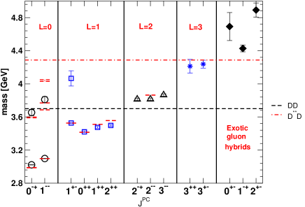
Figure 4: Charmonium spectrum from Reference Liao:2002rj . The rightmost three points correspond to the hybrid states.

4 $B$ physics

The strongest motivation for the lattice simulation of heavy quarks comes from $B$ physics. One of the goals of the $B$ factory experiments is to precisely determine the CKM matrix elements, which are fundamental parameters of the Standard Model. In particular, the two smallest elements $V_{ub}$ and $V_{td}$ are interesting because they describe the mixing between first and third generations and are the source of $CP$ violation. Furthermore, by studying a variety of flavor-changing-neutral-current (FCNC) processes, which are suppressed in the Standard Model by the GIM mechanism, one may get insight into the physics beyond the Standard Model entering into the loop diagrams.

The bottom quark decay inside the $B$ meson is always accompanied by a gluon and quark cloud, which makes the extraction of fundamental parameters from experimental data difficult. Therefore, a model independent calculation of QCD effects by a theoretical method, such as lattice QCD, is essential.

Owing to the practical limitation of computer power, the momentum scale that lattice QCD can treat is limited to $\lesssim$ 1 GeV, which is why the effective theories as discussed in Section 2 are developed. Computer power also limits the momentum of initial and final state hadrons to be simulated on the lattice to $\lesssim$ 1 GeV, whereas in realistic $B$ decays the momentum of the daughter particles can be as large as $\sim m_{B}/2$. This means that only a limited range of kinematical space is covered by lattice QCD. Another important limitation of lattice calculation is that one cannot treat the multi-hadron final state on the lattice, because the relation between the correlator in the Euclidean space and the amplitude in the Minkowski space-time is non-trivial when more than one particles are involved. Therefore, the direct calculation of the decay amplitude of $B\rightarrow\pi\pi$, for instance, is far beyond the reach of present lattice calculation.

In the following section, we review the lattice calculation of several important $B$ meson matrix elements.

4.1 $B^{0}$-$\bar{B}^{0}$ Mixing

The mass difference (or oscillation frequency) between two neutral $B$ mesons $\Delta M_{B_{q}}$ ($q=d$ or $s$) is given by

$$\Delta M_{B_{q}}=\frac{G_{F}^{2}}{6\pi^{2}}\eta_{B}M_{B_{q}}f_{B_{q}}^{2}\hat{B}_{B_{q}}m_{W}^{2}S_{0}(m_{t}^{2}/m_{W}^{2})|V_{tq}V_{tb}|^{2},$$ (24)

where $S_{0}(x)$ is the Inami-Lim function Inami:1980fz originating from the box diagram and $\eta_{B}$ is a short distance QCD correction calculated in perturbative QCD. The non-perturbative quantity to be computed on the lattice is the combination, $f_{B_{q}}^{2}\hat{B}_{B_{q}}$. The leptonic decay constant $f_{B_{q}}$ is defined through

$$if_{B_{q}}p_{\mu}=\langle 0|A_{\mu}|B_{q}(p)\rangle,$$ (25)

with a heavy-light axial-vector current $A_{\mu}=\bar{q}\gamma_{5}\gamma_{\mu}b$. The $B$ parameter $B_{B_{q}}$ is defined as

$$\langle\bar{B}^{0}_{q}|O^{\Delta B=2}(\mu)|B_{q}^{0}\rangle\equiv\frac{8}{3}B_{B_{q}}(\mu)f_{B_{q}}^{2}M_{B_{q}}^{2}$$ (26)

with the $\Delta B=2$ operator

$$O^{\Delta B=2}=\bar{q}\gamma_{\mu}(1-\gamma_{5})b\,\bar{q}\gamma_{\mu}(1-\gamma_{5})b.$$ (27)

This operator has an anomalous dimension, and as a result the $B$ parameter is scale dependent, $B_{B_{q}}(\mu)$. For convenience a scale-invariant $B$ parameter, $\hat{B}_{B_{q}}=B_{B_{q}}\alpha_{s}(\mu)^{-6/23}(1+J_{5}\alpha_{s}/4\pi)$, with $J_{5}=5165/3174$, is often quoted.

Experimentally, the mass difference $\Delta M_{B}$ is already known very precisely for the $B_{d}^{0}$ meson ($\Delta M_{B}=0.502\pm 0.007$ ps^-1 HFAG ), and the main problem in extracting the CKM element $|V_{td}|$ is in the theoretical calculation of $f_{B}^{2}B_{B}$. For the $B_{s}$ meson, to date only a lower bound $\Delta M_{s}>$ 14.4 ps^-1 (95% CL) HFAG has been obtained. The leptonic decay $B^{+}\to l\nu_{l}$ is hard to measure at existing experimental facilities because of its small branching fraction, although there is a good chance that it will be measured and thus a combination $|V_{ub}|f_{B}$ will be determined at future higher luminosity $B$ factories.

Because the $B_{d}$ and $B_{s}$ mesons differ only in the valence light quark mass as far as QCD is concerned, one can expect that the theoretical uncertainty largely cancels in the ratio

$$\frac{\Delta M_{B_{s}}}{\Delta M_{B_{d}}}=\frac{|V_{ts}|^{2}}{|V_{td}|^{2}}\xi^{2},\;\;\;\;\xi\equiv\frac{f_{B_{s}}\sqrt{B_{B_{s}}}}{f_{B_{d}}\sqrt{B_{B_{d}}}}$$ (28)

up to the SU(3) breaking effect. Once the $B_{s}$-$\bar{B}_{s}$ mixing rate is experimentally measured with good precision, it will help to determine the most interesting CKM matrix element $|V_{td}|$ (assuming the CKM unitarity relation $|V_{ts}|=|V_{cb}|$).

The width difference $\Delta\Gamma_{s}$ of $B_{s}$ mesons is induced by the final states into which both $B_{s}$ and $\bar{B}_{s}$ mesons can decay. (The width difference of $B_{d}$ in the Standard Model is too small to be observed.) The main contribution comes from $\bar{b}s\to c\bar{c}\to b\bar{s}$ transitions at the quark level. Because large momentum of order $m_{b}/2$ flows into final state particles, the amplitude can be expressed in terms of the heavy quark expansion Beneke:1996gn ; Beneke:1998sy and the leading order is represented by matrix elements of local $\Delta B=2$ four-quark operators $O_{L}=\bar{s}\gamma_{\mu}(1-\gamma_{5})b\,\bar{s}\gamma_{\mu}(1-\gamma_{5})b$ and $O_{S}=\bar{s}(1-\gamma_{5})b\,\bar{s}(1-\gamma_{5})b$. The corresponding matrix elements are $B_{B}$ and $B_{S}$, defined such that they are unity in the vacuum saturation approximation.

4.2 $B^{0}$-$\bar{B}^{0}$ Mixing: Quenched Lattice Results

In the quenched approximation, the $B$ meson decay constant has been studied extensively. Recent calculations using the Fermilab action Aoki:ji ; El-Khadra:1997hq ; Bernard:1998xi , the NRQCD action AliKhan:1998df ; Ishikawa:1999xu ; Collins:2000ix ; AliKhan:2001jg , and the extrapolation method Becirevic:1998ua ; Bowler:2000xw ; Lellouch:2000tw show good agreement within an error of $O(15\%)$. In the recent lattice conferences, world averages read $f_{B}=173\pm 23$ MeV, $f_{B_{s}}=200\pm 20$ MeV, and $f_{B_{s}}/f_{B_{d}}=1.15\pm 0.03$ Ryan:2001ej ; Yamada:2002wh . The statistical error of the Monte Carlo simulation is a minor part of the error given above. The source of systematic error differs significantly according to the method used to treat the heavy quark. In the Fermilab and NRQCD actions, the truncation of the perturbative and non-relativistic expansions is a major source of uncertainty. For the extrapolation method, the matching factor is known non-perturbatively and the non-relativistic expansion is not involved, but the extrapolation in the inverse heavy quark mass is a serious source of systematic error, as we discussed in Section 2. In addition, there is an error associated with the scale setting of the lattice, which is done by using some reference quantity—such as the rho meson mass, the pion (or kaon) decay constant, the string tension (or the “Sommer scale” $r_{0}$ which is also related to the heavy quark potential Sommer:1993ce ), and the quarkonium mass spectra. In the quenched approximation the lattice scales determined from different quantities do not necessarily agree. This is a potential source of systematic uncertainty.

More recently, there has been an attempt to control the $O[(am_{Q})^{2}]$ error by performing the simulations on a small physical volume, such as (0.4 fm)³, and matching the results to larger lattices recursively deDivitiis:2003wy . The result $f_{B_{s}}=192\pm 6\pm 4$ MeV agrees with the previous calculations and the quoted error is significantly smaller than the present world average. Another attempt is a further refinement of the extrapolation method Rolf:2003mn . By taking the continuum limit at each heavy quark mass, Rolf et al. eliminate the leading $O[(am_{Q})^{2}]$ error. The combined fit with the static result, which is also extrapolated to the continuum limit, yields a preliminary result $f_{B_{s}}=206\pm 10$ MeV Rolf:2003mn . By continuing in these and other directions, it will be possible to reduce the error in $f_{B}$ to the 5% level.

The $B$ parameters have been calculated on quenched lattices via the static action Ewing:1995ih ; Christensen:1996sj ; Gimenez:1996sk ; Gimenez:1998mw , the NRQCD action Hashimoto:1999ck ; Hashimoto:2000eh ; Aoki:2002bh , and the extrapolation method Becirevic:2000nv ; Lellouch:2000tw , for which the systematic error is better controlled by a combined fit with the static results Becirevic:2001xt . Their results are consistent with each other, and the current average is $\hat{B}_{B}=1.33\pm 0.12$ Yamada:2002wh .

The other $B$ parameter $B_{S}$, which is relevant to the $B_{s}$ meson width difference, has also been calculated in the quenched approximation Hashimoto:1999yh ; Hashimoto:2000eh ; Aoki:2002bh ; Becirevic:2000sj ; Gimenez:2000jj ; Flynn:2000hx ; Becirevic:2001xt . The physical result for $\Delta\Gamma_{s}/\Gamma_{s}$ including next-to-leading order QCD corrections is $0.074\pm 0.024$ Ciuchini:2003ww , which can be compared to the current experimental average $0.07^{+0.09}_{-0.07}$ HFAG .

4.3 $B^{0}$-$\bar{B}^{0}$ Mixing: Unquenching

In the past few years, the unquenched calculation of $f_{B}$ has been performed by several groups Bernard:1998xi ; Collins:1999ff ; AliKhan:2000eg ; AliKhan:2001jg , and the results seemed larger than the quenched results by $\sim$ 10%–15%. But the conclusion is now less clear because of an uncertainty in the chiral extrapolation as we discuss below.

With the present algorithms to incorporate the effect of dynamical fermions the simulation cost increases as $1/m_{q}^{3}$, where $m_{q}$ is the light quark mass Ukawa:pc . For example, for Wilson-type fermions the smallest possible sea quark mass is about a half of the strange quark mass $m_{s}$ even on the fastest available supercomputer. Hence, one must extrapolate the lattice data from the light quark mass region $m_{q}\gtrsim m_{s}/2$ toward the physical up and down quark masses, which are about $m_{s}/25$. In such an extrapolation the theoretical guide to restrict its functional form is given by chiral perturbation theory (ChPT) Gasser:1983yg ; Gasser:1984gg , which provides a systematic framework to calculate physical quantities as an expansion around the massless limit with an expansion parameter $m_{\pi}^{2}\propto m_{q}$. At next-to-leading (one-loop) order, ChPT predicts non-analytic behavior coming from pion loops. For instance, for the pion decay constant the non-analytic term is $-\frac{N_{f}}{2}\frac{m_{\pi}^{2}}{(4\pi f)^{2}}\ln\frac{m_{\pi}^{2}}{\mu^{2}}$ which is called the chiral logarithm. ($f$ is the pion decay constant in the massless limit.) Its coefficient depends only on the number of dynamically active quark flavors $N_{f}$, which is a consequence of the chiral symmetry of QCD.

The chiral logarithm could complicate the analysis of lattice data, because the effect of such non-analytic functional dependence can be missed if one simply relies on a polynomial fit of lattice data. Furthermore, when the lattice data are available only in the relatively heavy mass region $m_{q}\gtrsim m_{s}/2$, the convergence of the chiral expansion itself is questionable. An explicit study using $N_{f}=2$ lattice data from Reference Aoki:2002uc suggests that the region $m_{q}\gtrsim m_{s}/2$ is beyond the reach of ChPT Hashimoto:2002vi . If this is true, one must introduce some model function to fit the lattice data, in order to make the chiral extrapolation consistent with ChPT, which introduces significant uncertainty in the chiral extrapolation.

The heavy mesons can be incorporated into the framework of ChPT. At next-to-leading order Grinstein:1992qt , the $B$ meson decay constant depends on the light quark mass as follows:

$$\frac{\Phi_{f_{B}}}{\Phi_{f_{B}}^{(0)}}=1-\frac{3(1+3g^{2})}{4}\frac{m_{\pi}^{2}}{(4\pi f)^{2}}\ln\frac{m_{\pi}^{2}}{\mu^{2}}+c_{1}m_{\pi}^{2}+\cdots.$$ (29)

Here, $\Phi_{f_{B}}\equiv f_{B}\sqrt{M_{B}}$ and $\Phi_{f_{B}}^{(0)}$ denotes its value in the massless light quark limit. The coupling $g$ describes the $B^{*}B\pi$ interaction in ChPT, which is experimentally measured through the $D^{*}\to D\pi$ decay as $g=0.59\pm 0.01\pm 0.07$ Ahmed:2001xc ; Anastassov:2001cw , if heavy quark symmetry is assumed.

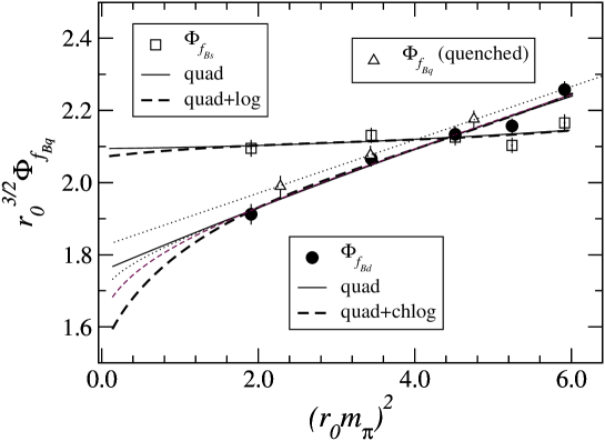
Figure 5: Chiral extrapolation of $\Phi_{f_{B_{d}}}$ (filled circles) and $\Phi_{f_{B_{s}}}$ (open squares). A polynomial fit is shown by solid lines; the fits with the hard cutoff chiral logarithm are shown for $\mu$ = 300 (dotted curve), 500 (thin dashed curve) and $\infty$ (thick dashed curve) MeV. Quenched results are also shown (triangles). The plot is from Reference Aoki:2003xb .

Figure 5 shows the chiral extrapolation of $\Phi_{f_{B_{d}}}$. The lattice data are from a recent unquenched simulation with two flavors of the $O(a)$-improved Wilson fermion Aoki:2003xb . The NRQCD action is used for the heavy quark. In order to estimate the systematic uncertainty associated with the chiral logarithm, the lattice results are fitted with Equation 29, but the chiral logarithm term is modified as $m_{\pi}^{2}\ln m_{\pi}^{2}/\mu^{2}\rightarrow m_{\pi}^{2}\ln m_{\pi}^{2}/(m_{\pi}^{2}+\mu^{2})$. This functional form is motivated by a hard cutoff regularization of one-loop ChPT; it is designed such that the effect of the pion loop is suppressed above the cutoff scale $\mu$, whereas Equation 29 is reproduced when $m_{\pi}^{2}\ll\mu^{2}$. By taking a maximum parameter range $\mu=0\to\infty$ MeV, the results obtained are $f_{B_{d}}=191(10)(^{+12}_{-22})$ MeV, $f_{B_{s}}=215(9)(^{+14}_{-13})$ MeV, and $f_{B_{s}}/f_{B_{d}}=1.13(3)(^{+13}_{-\ 2})$, where the first error is statistical, and the second is the estimate of the uncertainty due to chiral extrapolation and other sources added in quadrature Aoki:2003xb . Because the $f_{B_{s}}$ is hardly affected by the chiral logarithm, a large uncertainty remains only in $f_{B_{d}}$. The SU(3) breaking ratio $f_{B_{s}}/f_{B_{d}}$ contains significantly larger error than what was often reported in the quenched calculation, for which the effect of chiral logarithm was ignored.

The problem of large uncertainty due to the chiral logarithm was also emphasized in References Yamada:2001xp ; Kronfeld:2002ab . A possible way to reduce the error is to extrapolate a ratio $f_{B}/f_{\pi}$ instead of the individual decay constants Becirevic:2002mh . Because the coefficient of the chiral logarithm terms in $f_{B}$ and $f_{\pi}$ are numerically close, the uncertainty from the extrapolation will become smaller. For the cancellation of the chiral logarithms, a more natural choice is to consider $f_{B}/f_{D}$ or the Grinstein ratio $(f_{B_{s}}/f_{B})/(f_{D_{s}}/f_{D})$ Grinstein:1993ys , in which the chiral logarithm exactly cancels at the leading order of the $1/M$ expansion. These ratios are useful because the CLEO-c, an experimental progrom at Cornell, promises to measure $f_{D}$ and $f_{D_{s}}$ with a precision of a few per cent in a few years. An unquenched lattice calculation of the Grinstein ratio has already been attempted aiming at a few per cent accuracy Onogi:jn .

To be convincing, however, the unquenched simulations must employ much smaller sea quark masses. With currently available computational resources, only staggered fermions are feasible as dynamical fermions to carry out such simulations. The first such calculation including the dynamical effects of one strange and two light quarks was presented recently for $f_{B_{s}}$ Wingate:2003gm . The lightest sea quark mass is as small as $m_{s}/4$ in this work. The result, $f_{B_{s}}=260\pm 29$ MeV, is somewhat larger than the previous two-flavor result.

The $B$ parameter is also calculated in Reference Aoki:2003xb . The chiral logarithm is less problematic here, because the coefficient of the one-loop chiral log term is $-(1-3g^{2})/2$ rather than $3(1+3g^{2})/4$ in Equation 29 Sharpe:1995qp and is numerically negligible in practice. Results for the physically relevant quantities are $f_{B_{d}}\sqrt{\hat{B}_{B_{d}}}=215(11)(^{+15}_{-27})$ MeV, $f_{B_{s}}\sqrt{\hat{B}_{B_{s}}}=245(10)(^{+19}_{-17})$ MeV, and $\xi=1.14(3)(^{+13}_{-\ 2})$.

4.4 $B\to D^{(*)}l\nu$ Form Factors

The semi-leptonic decays $b\to cl\nu$ and $b\to ul\nu$ may be used to determine the CKM matrix elements $|V_{cb}|$ and $|V_{ub}|$ respectively, if their decay rates are theoretically calculated in a model independent way. For the exclusive decay modes, such as $B\to D^{(*)}l\nu$ and $B\to\pi l\nu$, the quantities to be calculated are their form factors.

For the heavy-to-heavy decays, namely $B\to D^{(*)}l\nu$, one can use the heavy quark symmetry to restrict their form factors, i.e. several form factors with different spin structures are related to one universal form factor called the Isgur-Wise function Isgur:vq ; Isgur:ed . Furthermore, thanks to the symmetry between the initial and final states, the form factor is normalized to unity in the kinematical end point where the daughter $D^{(*)}$ meson does not have spatial momentum in the rest frame of the initial $B$ meson. Specifically, if one writes the differential decay rate in terms of $w\equiv v\cdot v^{\prime}$ ($v$ and $v^{\prime}$ are the four-velocity of $B$ and $D^{*}$ mesons, respectively)

$$\frac{d\Gamma(B\to D^{*}l\nu)}{dw}=\frac{G_{F}^{2}|V_{cb}|^{2}m_{B}^{5}}{48\pi^{3}}\mathcal{K}(w)\mathcal{F}(w)^{2}$$ (30)

with $\mathcal{K}(w)$ a known kinematical factor, then the form factor $\mathcal{F}(w)$ obeys $\mathcal{F}(1)=1$. The CKM element $|V_{cb}|$ can thus be determined through the $w\to 1$ limit of experimental data.

However, because the heavy quark symmetry is exact only in the limit where both heavy quarks have infinite mass, one must take the $1/m$ corrections into account. Again using the heavy quark symmetry one can show that the leading correction to the relevant form factor $h_{A_{1}}(1)$, which is identical to $\mathcal{F}(1)$ in the zero-recoil limit, is $O(1/m^{2})$ Luke:1990eg :

$$h_{A_{1}}(1)=\eta_{A}[1+\delta_{1/m^{2}}+\delta_{1/m^{3}}],$$ (31)

with $\eta_{A}$ a short distance correction that comes from the matching between QCD and HQET, and

$$\delta_{1/m^{2}}=-\frac{\ell_{V}}{(2m_{c})^{2}}+\frac{2\ell_{A}}{2m_{c}2m_{b}}-\frac{\ell_{P}}{(2m_{b})^{2}}.$$ (32)

The parameters $\ell_{P}$, $\ell_{V}$, and $\ell_{A}$ are non-perturbative quantities, which were previously estimated using the non-relativistic quark model Falk:1992wt ; Neubert:1994vy .

These three parameters appear in the $1/m$ expansions of other form factors because of the heavy quark symmetry Falk:1992wt ; Mannel:1994kv , and thus can be obtained from lattice calculation of double ratios of zero recoil matrix elements Hashimoto:2001nb ; Kronfeld:2000ck

$$\frac{\langle D|\bar{c}\gamma^{4}b|\bar{B}\rangle\langle\bar{B}|\bar{b}\gamma^{4}c|D\rangle}{\langle D|\bar{c}\gamma^{4}c|D\rangle\langle\bar{B}|\bar{b}\gamma^{4}b|\bar{B}\rangle} = \left\{\eta_{V}^{\mathrm{lat}}[1-\ell_{P}\Delta+O(1/m^{3})]\right\}^{2},$$ (33)

$$\frac{\langle D^{*}|\bar{c}\gamma^{4}b|\bar{B}^{*}\rangle\langle\bar{B}^{*}|\bar{b}\gamma^{4}c|D^{*}\rangle}{\langle D^{*}|\bar{c}\gamma^{4}c|D^{*}\rangle\langle\bar{B}^{*}|\bar{b}\gamma^{4}b|\bar{B}^{*}\rangle}, = \left\{\eta_{V}^{\mathrm{lat}}[1-\ell_{V}\Delta+O(1/m^{3})]\right\}^{2},$$ (34)

$$\frac{\langle D^{*}|\bar{c}\gamma^{j}\gamma^{5}b|\bar{B}\rangle\langle\bar{B}^{*}|\bar{b}\gamma^{j}\gamma^{5}c|D\rangle}{\langle D^{*}|\bar{c}\gamma^{j}\gamma^{5}c|D\rangle\langle\bar{B}^{*}|\bar{b}\gamma^{j}\gamma^{5}b|\bar{B}\rangle} = \left\{\eta_{A}^{\mathrm{lat}}[1-\ell_{A}\Delta+O(1/m^{3})]\right\}^{2},$$ (35)

where $\Delta\equiv(1/(2m_{c})-1/(2m_{b}))$. The terms $\eta_{V}^{\mathrm{lat}}$ and $\eta_{A}^{\mathrm{lat}}$ are matching factors between lattice theory and continuum HQET Harada:2001fj . The double ratios of matrix elements can be precisely calculated, because both statistical and systematic errors largely cancel in the ratio. In the quenched approximation, $\mathcal{F}(1)=0.913^{+0.024+0.017}_{-0.017-0.030}$ has been obtained Hashimoto:2001nb . This may be compared to the quark model result Neubert:1994vy combined with a two-loop calculation of $\eta_{A}$ Czarnecki:1996gu ; Czarnecki:1997cf , namely $0.907\pm 0.031$, or the QCD sum rule result Shifman:jh ; Bigi:ga ; Uraltsev:2000qw $0.900\pm 0.038$.

The corresponding form factor $\mathcal{G}(1)$ for $B\to Dl\nu$ is written as

$$\mathcal{G}(1)=h_{+}(1)-\frac{m_{B}-m_{D}}{m_{B}+m_{D}}h_{-}(1),$$ (36)

using the form factors $h_{+}$ and $h_{-}$ defined through

$$\langle D(v^{\prime})|\bar{c}\gamma^{\mu}b|B(v)\rangle=\sqrt{m_{B}m_{D}}[(v+v^{\prime})h_{+}(w)+(v-v^{\prime})h_{-}(w)].$$ (37)

The lattice calculation is more involved because it contains $h_{-}(1)$, which cannot be obtained merely from the zero recoil matrix elements, but is possible using a similar technique Hashimoto:1999yp .

The Isgur-Wise function $\xi(w)$, which is a heavy quark limit of $h_{+}(w)$, can also be calculated on the lattice as a function of $w$. The lattice version of HQET that includes finite velocity was developed for this purpose Mandula:ds and was extended to include $1/m$ corrections Hashimoto:1995in ; Sloan:1997fc ; Foley:2002qv . It is technically more difficult than the usual HQET, because the velocity receives finite renormalization, which must be determined from non-perturbative simulation Hashimoto:1995in ; Mandula:1997hb ; Christensen:1999gv . Lattice calculations using the relativistic fermion have also been attempted Bernard:1993ey ; Bowler:1995bp , but the control of systematic error at the level of a few percent (the precision necessary for the determination of $|V_{cb}|$) is still challenging.

4.5 $B\to\pi l\nu$ form factors

Because the symmetry between the initial and final states is lost in the heavy-to-light decays, the form factors are no longer normalized for $B\to\pi l\nu$ or $\rho l\nu$. Therefore, lattice QCD must deal with the form factors themselves rather than just their $1/m$ expansion coefficients.

The $B\to\pi l\nu$ form factors $f^{+}(q^{2})$ and $f^{0}(q^{2})$ are defined through

$$\langle\pi(k)|\bar{q}\gamma^{\mu}b|B(p)\rangle=f^{+}(q^{2})\left[(p+k)^{\mu}-\frac{m_{B}^{2}-m_{\pi}^{2}}{q^{2}}q^{\mu}\right]+f^{0}(q^{2})\frac{m_{B}^{2}-m_{\pi}^{2}}{q^{2}}q^{\mu},$$ (38)

where $p$ and $k$ are the momenta of the initial $B$ and final $\pi$ mesons respectively, and $q^{\mu}=(p-k)^{\mu}$ is a momentum transfer to the lepton pair. The minimum value of $q^{2}$, namely zero, occurs when the lepton and neutrino are parallel and the pion is energetically propelled to the opposite direction. The maximum value $q^{2}_{\mathrm{max}}=(m_{B}-m_{\pi})^{2}$ occurs when the lepton and neutrino are emitted back-to-back with maximum energy and the pion stays at rest. The differential decay rate is written as

$$\frac{d\Gamma(B\to\pi l\nu)}{dq^{2}}=\frac{G_{F}^{2}}{24\pi^{3}}|V_{ub}|^{2}[(v\cdot k)^{2}-m_{\pi}^{2}]^{3/2}|f^{+}(q^{2})|^{2}.$$ (39)

Because the discretization error becomes uncontrollable for momenta much larger than $\Lambda_{\mathrm{QCD}}$, the calculation of the form factors is feasible only in the large $q^{2}$ (small recoil) region ($q^{2}\gtrsim$ 15 GeV²), where the spatial momentum of the pion is lower than roughly 1 GeV/c. The CKM matrix element $|V_{ub}|$ can be obtained by combining the experimental data integrated above some $q^{2}$ value, say 15 GeV², and the lattice results for the form factor $|f^{+}(q^{2})|^{2}$ integrated in the same region with an appropriate kinematical factor.

Extrapolation or interpolation in the heavy quark mass is done according to the heavy quark scaling law $f^{+}(q^{2})\sim\sqrt{m_{B}}$ and $f^{0}(q^{2})\sim 1/\sqrt{m_{B}}$. The analysis can be more explicit if one works with the HQET motivated form factors $f_{1}(v\cdot k)$ and $f_{2}(v\cdot k)$. These are defined in the heavy quark limit as Burdman:1993es

$$\langle\pi(k)|\bar{q}\gamma^{\mu}b|B(v)\rangle=2\left[f_{1}(v\cdot k)v^{\mu}+f_{2}(v\cdot k)\frac{k^{\mu}}{v\cdot k}\right]$$ (40)

where $v^{\mu}=p^{\mu}/m_{B}$ is the four-velocity of the $B$ meson. $f^{+}(q^{2})$ and $f^{0}(q^{2})$ are given by a linear combination of $f_{1}(v\cdot k)$ and $f_{2}(v\cdot k)$.

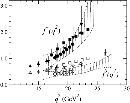
Figure 6: $q^{2}$ dependence of $B\rightarrow\pi l\nu$ form factors $f^{+}(q^{2})$ (filled symbols) and $f^{0}(q^{2})$ (open symbols). Upward triangles, downward triangles, squares, circles denote data from the UKQCD Bowler:1999xn , APE Abada:2000ty , Fermilab El-Khadra:2001rv and JLQCD Aoki:2001rd collaborations, respectively.

Recently, five groups have carried out extensive quenched calculations of $B\to\pi l\nu$ form factors using the extrapolation method Bowler:1999xn ; Abada:2000ty , the Fermilab action El-Khadra:2001rv , and the NRQCD action Aoki:2001rd ; Shigemitsu:2002wh for heavy quarks. Results for the form factors $f^{+}(q^{2})$ and $f^{0}(q^{2})$ are shown in Figure 6. Overall, results for $f^{+}(q^{2})$ are in agreement among four different groups within the error of order 20%, but some disagreement is observed for $f^{0}(q^{2})$. It originates from differences in the light quark mass dependence of the data. Further understanding is necessary to resolve these differences.

The chiral extrapolation is more problematic for these form factors than for the decay constant, since the reference point $q^{2}$ (or $v\cdot k$) also varies with the light quark mass. If one sticks to a particular kinematical point, e.g., the zero recoil, the extrapolation must include a linear term in $m_{\pi}$ in addition to the usual $m_{\pi}^{2}$ term. In fact, the soft pion relation $f^{0}(q^{2})=f_{B}/f_{\pi}$ is poorly satisfied unless the extrapolation includes the linear $m_{\pi}$ term Aoki:2001rd . Furthermore, the chiral logarithm Fleischer:1992tn ; Becirevic:2002sc must be taken into account in future unquenched calculations. Some unquenched studies are in progress, especially using staggered dynamical quarks Shigemitsu:2003xw ; Bernard:2003gu ; Okamoto:2003ur .

4.6 $B\to\rho l\nu$ and other form factors

The decay $B\to\rho l\nu$ can also be used to determine $|V_{ub}|$. However, the lattice calculation of its form factors is more complicated than for $B\to\pi l\nu$, because there are four (not two) independent form factors corresponding to different spin-momentum combinations. Furthermore, the statistical signal of the Monte Carlo simulation is significantly worse for the rho meson, especially when finite spatial momentum is injected. A more fundamental problem is that the rho meson is an unstable particle that has a large width $\sim$ 150 MeV. Lattice simulations of such an unstable particles should eventually treat the two-pion final states and take its phase shift into account, the practical feasibility of which is still an open question.

Figure 7: Differential decay rate of the $B\to\rho l\nu$ mode. Lattice data are shown with a fit curve discussed in the text. (From Reference Flynn:1995dc with permission).

Despite these problems, it is worth calculating those form factors on the lattice because the calculation provides a firmer theoretical guide for the experimental analysis than do the previous model calculations. A study was made by the UKQCD collaboration using the extrapolation method Flynn:1995dc . (Earlier works on $D\to K^{(*)}l\nu$ decays inculde References Lubicz:1991bi ; Bernard:fg ; Bernard:bz ; Bowler:1994zr .) As in the $B\to\pi l\nu$ form factors the lattice calculation is reliable only in the high $q^{2}$ region. The extraction of $|V_{ub}|$ can be made by combining a partially integrated decay rate with the lattice results in the corresponding region. The differential decay rate is written as

$$\frac{d\Gamma(B\to\rho l\nu)}{dq^{2}}=\frac{G_{F}^{2}|V_{ub}|^{2}}{192\pi^{3}m_{B}^{3}}q^{2}[\lambda(q^{2})]^{1/2}\left(|H^{+}(q^{2})|^{2}+|H^{-}(q^{2})|^{2}+|H^{0}(q^{2})|^{2}\right),$$ (41)

where $\lambda(q^{2})$ is a kinematical factor. $H^{0}(q^{2})$ and $H^{\pm}(q^{2})$ denote amplitudes with longitudinal and transverse rho meson polarization, respectively, and are written in terms of three form factors $A_{1}(q^{2})$, $A_{2}(q^{2})$ and $V(q^{2})$. Near the $q^{2}_{\mathrm{max}}$ one can parametrize these amplitudes as $a^{2}(1+b(q^{2}-q^{2}_{\mathrm{max}}))$. Figure 7 shows the lattice results for the differential decay rate with a fit curve using the above parametrization. It demonstrates how lattice calculation can be used to compare theory with experiments.

The systematic error is still as large as $\sim$ 25% from the $1/M$ extrapolation and other sources. The calculation is in the quenched approximation and the chiral limit of the valence light quark is yet to be taken. These problems are being addressed. Indeed, a couple of large scale quenched lattice calculations are in progress using the extrapolation method Gill:2001jp ; Abada:2002ie , and they have already reported preliminary results.

Phenomenologically, the FCNC processes $b\to s(d)\gamma$ and $b\to s(d)l^{+}l^{-}$ are also interesting because they occur through penguin and box diagrams, which are sensitive to possible new-physics contributions. Their exclusive decay modes are $B\to K^{*}\gamma$, $B\to\rho\gamma$, $B\to K^{(*)}l^{+}l^{-}$, and $B\to K^{(*)}\nu\bar{\nu}$. For the radiative decays $B\to K^{*}\gamma$ and $\rho\gamma$ the lattice calculation of the form factor necessarily involves some model dependence, since the form factor at $q^{2}=0$ is relevant. One must therefore extrapolate the lattice data from the high $q^{2}$ region assuming some functional form of the $q^{2}$ dependence, as was done in References Bowler:cq ; Burford:1995fc .

For the $B\to K^{(*)}l^{+}l^{-}$ and $B\to K^{(*)}\nu\bar{\nu}$ decays, on the other hand, the lattice calculation may be useful in the large lepton invariant mass region. However, the long distance effect due to $q\bar{q}$ and $c\bar{c}$ resonances must be taken into account for the $l^{+}l^{-}$ final states.

4.7 HQET Parameters

The HQET parameters, defined as

$$\mu_{\pi}^{2}(H_{Q}) \equiv \frac{1}{2M_{H_{Q}}}\left\langle H_{Q}\left|\bar{Q}(i\mbox{\boldmath$D$})^{2}Q\right|H_{Q}\right\rangle,$$ (42)

$$\mu_{G}^{2}(H_{Q}) \equiv \frac{1}{2M_{H_{Q}}}\left\langle H_{Q}\left|\bar{Q}\mbox{\boldmath$\sigma$}\cdot\mbox{\boldmath$B$}Q\right|H_{Q}\right\rangle,$$ (43)

appear in the analysis of the heavy quark expansion Neubert:1997gu ; Bigi:1997fj . For instance, the inclusive decay rate of a heavy hadron $H_{Q}$ is written as

$$\Gamma(H_{Q}\rightarrow X_{f})=\frac{G_{F}^{2}m_{Q}^{5}}{192\pi^{3}}\left[c_{3}^{f}\left(1-\frac{\mu_{\pi}^{2}(H_{Q})-\mu_{G}^{2}(H_{Q})}{2m_{Q}^{2}}\right)+2c_{5}^{f}\,\frac{\mu_{G}^{2}(H_{Q})}{m_{Q}^{2}}+\cdots\right],$$ (44)

where the coefficients $c_{3}^{f}$ and $c_{5}^{f}$ are perturbatively calculable Chay:1990da ; Bigi:1993fe ; Manohar:1993qn ; Blok:1993va . Because the leading order term is independent of the type of hadrons, it gives interesting predictions of lifetime ratios:

$$\frac{\tau(H_{b}^{(1)})}{\tau(H_{b}^{(2)})}=1+\frac{\mu_{\pi}^{2}(H_{b}^{(1)})-\mu_{\pi}^{2}(H_{b}^{(2)})}{2m_{b}^{2}}+c_{G}\frac{\mu_{G}^{2}(H_{b}^{(1)})-\mu_{G}^{2}(H_{b}^{(2)})}{m_{b}^{2}}+O\left(\frac{1}{m_{b}^{3}}\right),$$ (45)

with a perturbative coefficient $c_{G}\simeq$ 1.2 Neubert:1996we .

The parameters $\mu_{\pi}^{2}(H_{Q})$ and $\mu_{G}^{2}(H_{Q})$ are non-perturbative parameters that depend on heavy hadrons $H_{Q}$. Whereas the spin-dependent parameter $\mu_{G}^{2}(H_{Q})$ is reliably determined from the hyperfine splitting $m_{B^{*}}-m_{B}$, the determination of $\mu_{\pi}^{2}(H_{Q})$ requires non-perturbative methods, such as lattice QCD.

The lattice calculation of $\mu_{\pi}^{2}(H_{Q})$ suffers from the subtraction of the quadratic divergence that appears in the matching of the lattice operator $-\bar{Q}\mbox{\boldmath$D$}^{2}Q$ to its continuum counterpart. Because the perturbative subtraction involves large systematic error Martinelli:1996pk , a non-perturbative subtraction has been attempted and the result $\lambda_{1}=0.09\pm 0.14$ GeV² has been obtained Crisafulli:1995pg ; Gimenez:1996av . Another possible approach is to rely on the mass formula, such as $M_{\bar{B}}=m_{b}+\bar{\Lambda}-\lambda_{1}/2m_{b}$ for a spin-averaged 1S $B$ meson, and to fit the lattice data as a function of $1/m_{b}$. The results of such analysis using the NRQCD action AliKhan:1999yb and the Fermilab action Kronfeld:2000gk are $\lambda_{1}=-0.1\pm 0.4$ GeV² and $-0.45\pm 0.12$ GeV², respectively. In this method the quadratic divergence is subtracted away by the fitting, but the matching of the kinetic term in the non-relativistic expansion is a possible source of error. The reason for the disagreement with the above result with non-perturbative subtraction is not clear yet.

It is also possible to avoid the subtraction of the quadratic divergence by concentrating on the difference among different hadrons, e.g. $\mu_{\pi}^{2}(\Lambda_{b})-\mu_{\pi}^{2}(B)$, which is still useful in the estimate of lifetime ratios through Equation 45. A recent quenched calculation Aoki:2003jf , $\mu_{\pi}^{2}(\Lambda_{b})-\mu_{\pi}^{2}(B)=-0.01\pm 0.52$ GeV², is consistent with most phenomenological estimates. In particular, the well-known inconsistency of the heavy quark expansion of $\tau(\Lambda_{b})/\tau(B)\simeq 0.98$ with the experimental value $0.77\pm 0.05$ HFAG continues to be a problem. At the $1/m_{b}^{3}$ order, the spectator quark effect, which is expressed in terms of $\Delta B=0$ four-quark operators, becomes important Neubert:1996we . A lattice calculation DiPierro:1999tb of those matrix elements suggests that the spectator effects are indeed significant but not sufficiently large to account for the full discrepancy.

4.8 $B^{*}B\pi$ Coupling

The heavy quark symmetry and chiral symmetry can be combined into the framework of heavy meson ChPT Burdman:gh ; Wise:hn ; Yan:gz , which enables us to systematically expand physical amplitudes in terms of small pion momenta. This theory includes one additional parameter, $g$. It is related to the $B^{*}B\pi$ coupling $g_{B^{*}B\pi}$ defined by

$$\langle B(p)\pi(q)|B^{*}(p^{\prime})\rangle=-g_{B^{*}B\pi}q_{\mu}\eta^{\mu}(2\pi)^{4}\delta^{4}(p^{\prime}-p-q),$$ (46)

where $\eta^{\mu}$ is the polarization vector of the $B^{*}$ meson, and the $B^{*}B\pi$ coupling $g_{B^{*}B\pi}$ is proportional to the low energy constant $g$ as $g_{B^{*}B\pi}=2gm_{B}/f_{\pi}$. The analogous coupling in charmed mesons can be measured experimentally from the $D^{*}\to D\pi$ decay width, yielding $g=0.59\pm 0.01\pm 0.07$ Ahmed:2001xc ; Anastassov:2001cw . Using this value in $B$ physics is subject to uncertainties of order $\Lambda/m_{c}$.

At tree level, the coupling is related to the semi-leptonic $B\to\pi l\nu$ decay form factor $f^{+}(q^{2})$ in the large $q^{2}$ region. Using the soft pion theorem the form factor $f^{+}(q^{2})$ near $q^{2}\sim m_{B^{*}}^{2}$ behaves as

$$f^{+}(q^{2})=\frac{f_{B^{*}}}{2m_{B^{*}}}\frac{g_{B^{*}B\pi}}{(1-q^{2}/m_{B^{*}}^{2})}.$$ (47)

Thus, a precise knowledge of $g_{B^{*}B\pi}$ can constrain the CKM matrix element $|V_{ub}|$. The coupling $g$ also appears in the ChPT loop amplitudes as in the discussion of chiral extrapolation of $f_{B}$ in Section 4.3.

A direct lattice calculation of $g_{B^{*}B\pi}$ is possible if one modifies Equation 46 by using the soft pion theorem as a matrix element of the axial-vector current

$$\langle B(p)|q_{\mu}A^{\mu}|B^{*}(p^{\prime},\lambda)\rangle=g_{B^{*}B\pi}\frac{q\cdot\eta}{m_{\pi}^{2}-q^{2}}f_{\pi}m_{\pi}^{2},$$ (48)

where $q=p-p^{\prime}$. The lattice calculation of the matrix element on the left hand side is technically similar to the calculation of semi-leptonic form factors. A quenched calculation in the static limit was done several years ago and the result was $g=0.42\pm 0.04\pm 0.08$ deDivitiis:1998kj . More recently, Abada et al. performed an extensive calculation for the $D^{*}D\pi$ coupling Abada:2002xe and for $B^{*}B\pi$ in the heavy quark mass limit Abada:2003un . Their result $g=0.48\pm 0.03\pm 0.11$ Abada:2003un is consistent with the previous estimates. They also found that the $1/m_{Q}$ dependence is not significant.

4.9 Light-Cone Wave Function

As discussed in Section 4.5, $B$ decays with large recoil momentum are beyond the reach of current lattice calculations. Multi-hadron final states are even more difficult to treat on the lattice.

For these energetic decays, a more natural theoretical treatment is to factorize the energetic interaction, which is perturbatively calculable, and the non-perturbative physics, which is governed by the energy scale of order $\Lambda_{\mathrm{QCD}}$. Such a formalism was developed by Beneke et al. a few years ago Beneke:1999br ; Beneke:2001ev . For example, the amplitude of the non-leptonic $B\to\pi\pi$ decay is written as

$$\langle\pi(p^{\prime})\pi(q)|Q_{i}|B(p)\rangle = f^{B\to\pi}(q^{2})\int_{0}^{1}\!\!du\,T_{i}^{\mathit{I}}(u)\Phi_{\pi}(u)$$ (49)

$$+\int_{0}^{1}\!\!d\xi dudvT_{i}^{\mathit{II}}(\xi,u,v)\Phi_{B}(\xi)\Phi_{\pi}(u)\Phi_{\pi}(v).$$

Here $Q_{i}$ is a four-fermion operator and $T$’s are the perturbatively calculable short-distance part, whereas $f^{B\to\pi}$ is the $B\to\pi l\nu$ semi-leptonic decay form factor, and $\Phi$’s are the light-cone wave functions. Thus, the genuinely non-perturbative quantities are these light-cone wave functions.

There are lattice studies on the light-cone wave function of the pion. The light-cone wave function $\phi_{\pi}(u,Q^{2})$ is defined by the inverse Fourier transform of the matrix element

$$\langle 0|\bar{d}(0)e^{\int_{x}^{0}d\tau\cdot A(\tau)}\gamma_{\mu}\gamma_{5}u(x)|\pi^{+}(p)\rangle|_{p^{2}=0}=-ip_{\mu}f_{\pi}\int_{0}^{1}\!\!du\,e^{-ipx}\phi_{\pi}(u,Q^{2}).$$ (50)

The $n$-th moment of $\phi_{\pi}(u,Q^{2})$, defined as $\langle\xi^{n}\rangle\equiv\int_{0}^{1}d\xi\xi^{n}\phi_{\pi}(\xi,Q^{2})$, can be related to the pionic matrix element with the local bilinear operator with $n$ derivatives as follows:

$$\langle 0|\bar{d}\gamma_{\mu}\gamma_{5}\stackrel{{\scriptstyle\leftrightarrow}}{{D}}_{\mu_{1}}\cdots\stackrel{{\scriptstyle\leftrightarrow}}{{D}}_{\mu_{n}}u|\pi^{+}(p)\rangle=i^{n}f_{\pi}\,p_{\mu}p_{\mu_{1}}\cdots p_{\mu_{n}}\langle\xi^{n}\rangle.$$ (51)

The second moment of the light-cone wave function has been calculated by several lattice groups Gottlieb:ie ; DeGrand:1987vy ; Martinelli:1987si ; Martinelli:1987bh ; Daniel:1990ah ; DelDebbio:2002mq . A similar calculation is needed for the $B$ meson in order to establish contact with the $B$ physics phenomenology.

A more direct calculation of the light-cone wave function, not limited to its moments, has also been proposed Aglietti:1998ur . A pioneering numerical study has been carried out using this method Abada:2001if , which is worthy of further studies.

5 Future perspectives

Lattice QCD has many applications, but the flavor physics is where it plays a crucial role in the exploration of physics beyond the Standard Model through model independent calculation of weak matrix elements. Because the precision of the calculation is crucial in such studies, the systematic errors in the lattice calculation have to be well understood and reduced as much as possible. In the past decade many important steps have been made in this direction:

• $O(a)$-improvement of lattice actions and operators. The discretization errors are described by Symanzik’s effective theory, which also provides a method to improve lattice actions in a systematic way Symanzik:1983dc . It is now common to use the $O(a)$-improved action, for which the leading discretization error is $O(a^{2})$. Further improvement is also being pursued.

• Effective theory for heavy quarks. The ideas of HQET and NRQCD are naturally implemented on the lattice. The problem of dealing with heavy quarks on the lattice has essentially been solved Kronfeld:2002pi .

• Improved perturbation theory. Perturbation theory is still necessary in the lattice calculation to match the lattice action onto the target continuum theory. The convergence of the perturbative expansion was dramatically improved by the use of the renormalized coupling Lepage:1992xa .

The first two advances are related to the separation of different energy scales by the use of effective theories, and the third is needed for the matching of these effective theories.

We have reviewed the results that have relied on these methodological developments. One of the main challenges now is to further substantially reduce the systematic error. This could be achieved by pushing the idea of the effective theories, i.e. including the higher order improvement terms and higher order relativistic corrections. These have to be done together with the matching with the higher order perturbation theory. Although the higher order perturbative calculation is technically rather demanding on the lattice, some work is already in progress Trottier:2003bw . Another proposed way to reduce the systematic errors, which does not rely on perturbative matching, is the recursive non-perturbative matching methods deDivitiis:2003wy ; Heitger:2003nj .

To obtain truly model independent results from lattice QCD, the quenched approximation must be abandoned. Large scale simulations that include the effects of dynamical quarks have already been carried out by several lattice groups and will be performed more extensively in the future. One of the important effects of dynamical quarks is the pion loop effect, which leads to the chiral logarithm and affects the chiral extrapolation of lattice data in a non-trivial way. As a result, the systematic uncertainty due to the chiral extrapolation is still quite significant. Although our discussion on this problem used $f_{B}$ as an example, the same is true for almost all other lattice observables as long as their chiral behavior is known from ChPT. (Otherwise, there is no theoretical guide for the functional form of chiral extrapolation.) To eliminate the uncertainty from the chiral extrapolation, one must push the dynamical quark masses in the lattice simulations down to the region where the chiral logarithm becomes a visible effect. It is presumably lower than $m_{s}/3$. Such simulation is currently feasible only with the staggered fermion action for dynamical quarks, which is numerically so cheap that the MILC collaboration achieved even $m_{s}/6$. The results for several physical quantities agree with their experimental values quite remarkably Davies:2003ik . The price, however, is the introduction of fictitious species, sometimes called “tastes.” The taste breaking effect introduces an additional source of systematic uncertainty. Furthermore, in the dynamical simulation the fourth root of the fermionic determinant must be taken, and it is not known whether this gives a local field theory in the continuum limit Jansen:2003nt . These points are still controversial. Other lattice fermion formulations should also be pursued, for which the developments of simulation algorithms are essential.

As we have discussed, in order to achieve the goal of precise, model-independent simulation of heavy quarks, improvements are necessary throughout lattice QCD, i.e. from the higher order perturbative calculation to the simulation of really light dynamical quarks. Despite the difficulties, these future improvements will be worth the effort, because from an improved flavor physics one may probe physics beyond the Standard Model.

The application of lattice QCD to heavy quark physics is not limited to $f_{B}$ and $B_{B}$. Some other relevant quantities, such as semi-leptonic decay form factors and heavy quark expansion parameters, have already been studied on the lattice. There are, however, many other important quantities that require non-perturbative calculations. The FCNC processes $B\to K^{(*)}l^{+}l^{-}$ are sensitive to new physics, and hence the calculation of their form factors has direct relevance to the new-physics search. The two-body decays of the $B$ meson have become theoretically tractable since the factorization of short and long distance physics was proven. Non-perturbative inputs are necessary for the long distance part, which is the light-cone distribution function. Inclusive $B$ decays, such as $B\to X_{s}\gamma$ and $B\to X_{u}l\nu$, can be calculated perturbatively by using the heavy quark expansion, but in the kinematical region of interest the simple OPE breaks down, so that resummation of a certain class of higher-twist terms is necessary. Thus, a non-perturbative calculation of the quantity called the shape function, which describes the Fermi motion of the bottom quark, is required to predict their energy distributions. Aside from the $B$ decays, the heavy meson and baryon spectroscopy is also attracting attention, since the recent discovery of such exotic particles as $D_{sJ}(2317)$ and $X(3872)$. Lattice QCD is the prime tool for the non-perturbative study of these particles. All these applications will be investigated in the future.

References

- (1) K. G. Wilson, Phys. Rev. D 10, 2445 (1974).
- (2) S. L. Glashow, J. Iliopoulos and L. Maiani, Phys. Rev. D 2, 1285 (1970).
- (3) E. Eichten and B. Hill, Phys. Lett. B 234, 511 (1990).
- (4) H. Georgi, Phys. Lett. B 240, 447 (1990).
- (5) B. Grinstein, Nucl. Phys. B 339, 253 (1990).
- (6) W. E. Caswell and G. P. Lepage, Phys. Lett. B 167, 437 (1986).
- (7) B. A. Thacker and G. P. Lepage, Phys. Rev. D 43, 196 (1991).
- (8) G. P. Lepage, L. Magnea, C. Nakhleh, U. Magnea and K. Hornbostel, Phys. Rev. D 46, 4052 (1992) [arXiv:hep-lat/9205007].
- (9) A. X. El-Khadra and M. Luke, Ann. Rev. Nucl. Part. Sci. 52, 201 (2002) [arXiv:hep-ph/0208114].
- (10) C. W. Bernard, Nucl. Phys. Proc. Suppl. 94, 159 (2001) [arXiv:hep-lat/0011064].
- (11) S. M. Ryan, Nucl. Phys. Proc. Suppl. 106, 86 (2002) [arXiv:hep-lat/0111010].
- (12) N. Yamada, Nucl. Phys. Proc. Suppl. 119, 93 (2003) [arXiv:hep-lat/0210035].
- (13) A. S. Kronfeld, Nucl. Phys. Proc. Suppl. 129, 46 (2004) [arXiv:hep-lat/0310063].
- (14) J. M. Flynn and C. T. Sachrajda, in “Heavy Flavours (2nd ed.),” edited by A.J. Buras and M. Linder, World Scientific (1998); [arXiv:hep-lat/9710057].
- (15) A. S. Kronfeld, in “At the Frontiers of Particle Physics: Handbook of QCD Vol. 4,” edited by M. Shifman, World Scientific Publishing (2002); arXiv:hep-lat/0205021.
- (16) I. Montvay and G. Munster, “Quantum Fields on a Lattice,” Cambridge University Press (1994).
- (17) J. Smit, “Introduction to Quantum Fields on a Lattice,” Cambridge University Press (2002).
- (18) B. Sheikholeslami and R. Wohlert, Nucl. Phys. B 259, 572 (1985).
- (19) K. G. Wilson, Phys. Rev. 179, 1499 (1969).
- (20) A. X. El-Khadra, A. S. Kronfeld and P. B. Mackenzie, Phys. Rev. D 55, 3933 (1997) [arXiv:hep-lat/9604004].
- (21) A. S. Kronfeld, Phys. Rev. D 62, 014505 (2000) [arXiv:hep-lat/0002008].
- (22) S. Aoki, Y. Kuramashi and S. i. Tominaga, Prog. Theor. Phys. 109, 383 (2003) [arXiv:hep-lat/0107009].
- (23) C. T. H. Davies and B. A. Thacker, Phys. Rev. D 45, 915 (1992).
- (24) C. J. Morningstar, Phys. Rev. D 48, 2265 (1993) [arXiv:hep-lat/9301005].
- (25) C. J. Morningstar, Phys. Rev. D 50, 5902 (1994) [arXiv:hep-lat/9406002].
- (26) K. I. Ishikawa et al. [JLQCD Collaboration], Phys. Rev. D 61, 074501 (2000) [arXiv:hep-lat/9905036].
- (27) B. P. G. Mertens, A. S. Kronfeld and A. X. El-Khadra, Phys. Rev. D 58, 034505 (1998) [arXiv:hep-lat/9712024].
- (28) P. Boucaud, L. C. Lung and O. Pene, Phys. Rev. D 40, 1529 (1989).
- (29) E. Eichten and B. Hill, Phys. Lett. B 240, 193 (1990).
- (30) P. Boucaud, J. P. Leroy, J. Micheli, O. Pene and G. C. Rossi, Phys. Rev. D 47, 1206 (1993) [arXiv:hep-lat/9208004].
- (31) A. Borrelli and C. Pittori, Nucl. Phys. B 385, 502 (1992).
- (32) O. F. Hernandez and B. R. Hill, Phys. Lett. B 289, 417 (1992) [arXiv:hep-ph/9203221].
- (33) J. Heitger, M. Kurth and R. Sommer [ALPHA Collaboration], Nucl. Phys. B 669, 173 (2003) [arXiv:hep-lat/0302019].
- (34) C. T. H. Davies and B. A. Thacker, Phys. Rev. D 48, 1329 (1993).
- (35) C. J. Morningstar and J. Shigemitsu, Phys. Rev. D 57, 6741 (1998) [arXiv:hep-lat/9712016].
- (36) C. J. Morningstar and J. Shigemitsu, Phys. Rev. D 59, 094504 (1999) [arXiv:hep-lat/9810047].
- (37) J. Harada, S. Hashimoto, K. I. Ishikawa, A. S. Kronfeld, T. Onogi and N. Yamada, Phys. Rev. D 65, 094513 (2002) [arXiv:hep-lat/0112044].
- (38) J. M. Flynn, O. F. Hernandez and B. R. Hill, Phys. Rev. D 43, 3709 (1991).
- (39) M. Di Pierro and C. T. Sachrajda [UKQCD Collaboration], Nucl. Phys. B 534, 373 (1998) [arXiv:hep-lat/9805028].
- (40) V. Gimenez and J. Reyes, Nucl. Phys. B 545, 576 (1999) [arXiv:hep-lat/9806023].
- (41) K. I. Ishikawa, T. Onogi and N. Yamada, Phys. Rev. D 60, 034501 (1999) [arXiv:hep-lat/9812007].
- (42) S. Hashimoto, K. I. Ishikawa, T. Onogi, M. Sakamoto, N. Tsutsui and N. Yamada, Phys. Rev. D 62, 114502 (2000) [arXiv:hep-lat/0004022].
- (43) G. Martinelli and C. T. Sachrajda, Nucl. Phys. B 478, 660 (1996) [arXiv:hep-ph/9605336].
- (44) J. Heitger and R. Sommer [ALPHA Collaboration], JHEP 0402, 022 (2004) [arXiv:hep-lat/0310035].
- (45) J. Rolf and S. Sint [ALPHA Collaboration], JHEP 0212, 007 (2002) [arXiv:hep-ph/0209255].
- (46) A. Juttner and J. Rolf [ALPHA Collaboration], Phys. Lett. B 560, 59 (2003) [arXiv:hep-lat/0302016].
- (47) M. G. Alford, T. R. Klassen and G. P. Lepage, Nucl. Phys. B 496, 377 (1997) [arXiv:hep-lat/9611010].
- (48) J. Harada, A. S. Kronfeld, H. Matsufuru, N. Nakajima and T. Onogi, Phys. Rev. D 64, 074501 (2001) [arXiv:hep-lat/0103026].
- (49) S. Hashimoto and M. Okamoto, Phys. Rev. D 67, 114503 (2003) [arXiv:hep-lat/0302012].
- (50) C. T. H. Davies, K. Hornbostel, A. Langnau, G. P. Lepage, A. Lidsey, J. Shigemitsu and J. H. Sloan, Phys. Rev. D 50, 6963 (1994) [arXiv:hep-lat/9406017].
- (51) C. T. H. Davies, K. Hornbostel, G. P. Lepage, A. J. Lidsey, J. Shigemitsu and J. H. Sloan, Phys. Rev. D 52, 6519 (1995) [arXiv:hep-lat/9506026].
- (52) C. T. H. Davies, K. Hornbostel, G. P. Lepage, P. McCallum, J. Shigemitsu and J. H. Sloan, Phys. Rev. D 56, 2755 (1997) [arXiv:hep-lat/9703010].
- (53) C. T. H. Davies, K. Hornbostel, G. P. Lepage, A. Lidsey, P. McCallum, J. Shigemitsu and J. H. Sloan [UKQCD Collaboration], Phys. Rev. D 58, 054505 (1998) [arXiv:hep-lat/9802024].
- (54) G. P. Lepage, Nucl. Phys. Proc. Suppl. 26, 45 (1992).
- (55) T. Manke, I. T. Drummond, R. R. Horgan and H. P. Shanahan [UKQCD Collaboration], Phys. Lett. B 408, 308 (1997) [arXiv:hep-lat/9706003].
- (56) N. Eicker et al., Phys. Rev. D 57, 4080 (1998) [arXiv:hep-lat/9709002].
- (57) T. Manke et al. [CP-PACS Collaboration], Phys. Rev. D 62, 114508 (2000) [arXiv:hep-lat/0005022].
- (58) C. T. H. Davies et al. [HPQCD Collaboration], Phys. Rev. Lett. 92, 022001 (2004) [arXiv:hep-lat/0304004].
- (59) C. Davies and P. Lepage, arXiv:hep-ph/0311041.
- (60) K. Hagiwara et al. [Particle Data Group Collaboration], Phys. Rev. D 66, 010001 (2002).
- (61) H. D. Trottier, Phys. Rev. D 55, 6844 (1997) [arXiv:hep-lat/9611026].
- (62) N. H. Shakespeare and H. D. Trottier, Phys. Rev. D 58, 034502 (1998) [arXiv:hep-lat/9802038].
- (63) P. Chen, Phys. Rev. D 64, 034509 (2001) [arXiv:hep-lat/0006019].
- (64) M. Okamoto et al. [CP-PACS Collaboration], Phys. Rev. D 65, 094508 (2002) [arXiv:hep-lat/0112020].
- (65) S. Choe et al. [QCD-TARO Collaboration], JHEP 0308, 022 (2003) [arXiv:hep-lat/0307004].
- (66) G. T. Bodwin, E. Braaten and G. P. Lepage, Phys. Rev. D 51, 1125 (1995) [Erratum-ibid. D 55, 5853 (1997)] [arXiv:hep-ph/9407339].
- (67) G. T. Bodwin, D. K. Sinclair and S. Kim, Phys. Rev. Lett. 77, 2376 (1996) [arXiv:hep-lat/9605023].
- (68) G. T. Bodwin, D. K. Sinclair and S. Kim, Phys. Rev. D 65, 054504 (2002) [arXiv:hep-lat/0107011].
- (69) S. K. Choi et al. [Belle Collaboration], Phys. Rev. Lett. 91, 262001 (2003) [arXiv:hep-ex/0309032].
- (70) S. Perantonis and C. Michael, Nucl. Phys. B 347, 854 (1990).
- (71) C. Michael, arXiv:hep-ph/0308293.
- (72) K. J. Juge, J. Kuti and C. Morningstar, Phys. Rev. Lett. 90, 161601 (2003) [arXiv:hep-lat/0207004].
- (73) G. S. Bali and A. Pineda, Phys. Rev. D 69, 094001 (2004) [arXiv:hep-ph/0310130].
- (74) K. J. Juge, J. Kuti and C. J. Morningstar, Phys. Rev. Lett. 82, 4400 (1999) [arXiv:hep-ph/9902336].
- (75) T. Manke et al. [CP-PACS Collaboration], Phys. Rev. Lett. 82, 4396 (1999) [arXiv:hep-lat/9812017].
- (76) T. Manke et al. [CP-PACS Collaboration], Phys. Rev. D 64, 097505 (2001) [arXiv:hep-lat/0103015].
- (77) X. Liao and T. Manke, Phys. Rev. D 65, 074508 (2002) [arXiv:hep-lat/0111049].
- (78) X. Liao and T. Manke, arXiv:hep-lat/0210030.
- (79) T. Inami and C. S. Lim, Prog. Theor. Phys. 65, 297 (1981) [Erratum-ibid. 65, 1772 (1981)].
- (80) Heavy Flavor Averaging Group, http://www.slac.stanford.edu/xorg/hfag/index.html
- (81) M. Beneke, G. Buchalla and I. Dunietz, Phys. Rev. D 54, 4419 (1996) [arXiv:hep-ph/9605259].
- (82) M. Beneke, G. Buchalla, C. Greub, A. Lenz and U. Nierste, Phys. Lett. B 459, 631 (1999) [arXiv:hep-ph/9808385].
- (83) S. Aoki et al. [JLQCD Collaboration], Phys. Rev. Lett. 80, 5711 (1998).
- (84) A. X. El-Khadra, A. S. Kronfeld, P. B. Mackenzie, S. M. Ryan and J. N. Simone, Phys. Rev. D 58, 014506 (1998) [arXiv:hep-ph/9711426].
- (85) C. W. Bernard et al., Phys. Rev. Lett. 81, 4812 (1998) [arXiv:hep-ph/9806412].
- (86) A. Ali Khan et al. [CP-PACS Collaboration], Phys. Rev. D 64, 034505 (2001) [arXiv:hep-lat/0010009].
- (87) A. Ali Khan, S. Collins, C. T. H. Davies, C. Morningstar, J. Shigemitsu and J. H. Sloan, Phys. Lett. B 427, 132 (1998) [arXiv:hep-lat/9801038].
- (88) S. Collins, C. T. H. Davies, J. Hein, G. P. Lepage, C. J. Morningstar, J. Shigemitsu and J. H. Sloan, Phys. Rev. D 63, 034505 (2001) [arXiv:hep-lat/0007016].
- (89) A. Ali Khan et al. [CP-PACS Collaboration], Phys. Rev. D 64, 054504 (2001) [arXiv:hep-lat/0103020].
- (90) D. Becirevic, P. Boucaud, J. P. Leroy, V. Lubicz, G. Martinelli, F. Mescia and F. Rapuano, Phys. Rev. D 60, 074501 (1999) [arXiv:hep-lat/9811003].
- (91) K. C. Bowler, L. Del Debbio, J. M. Flynn, G. N. Lacagnina, V. I. Lesk, C. M. Maynard and D. G. Richards [UKQCD Collaboration], Nucl. Phys. B 619, 507 (2001) [arXiv:hep-lat/0007020].
- (92) L. Lellouch and C. J. D. Lin [UKQCD Collaboration], Phys. Rev. D 64, 094501 (2001) [arXiv:hep-ph/0011086].
- (93) R. Sommer, Nucl. Phys. B 411, 839 (1994) [arXiv:hep-lat/9310022].
- (94) G. M. de Divitiis, M. Guagnelli, F. Palombi, R. Petronzio and N. Tantalo, Nucl. Phys. B 672, 372 (2003) [arXiv:hep-lat/0307005].
- (95) J. Rolf et al. [ALPHA collaboration], Nucl. Phys. Proc. Suppl. 129, 322 (2004) [arXiv:hep-lat/0309072].
- (96) A. K. Ewing et al. [UKQCD Collaboration], Phys. Rev. D 54, 3526 (1996) [arXiv:hep-lat/9508030].
- (97) J. Christensen, T. Draper and C. McNeile, Phys. Rev. D 56, 6993 (1997) [arXiv:hep-lat/9610026].
- (98) V. Gimenez and G. Martinelli, Phys. Lett. B 398, 135 (1997) [arXiv:hep-lat/9610024].
- (99) S. Hashimoto, K. I. Ishikawa, H. Matsufuru, T. Onogi, S. Tominaga and N. Yamada, Phys. Rev. D 60, 094503 (1999) [arXiv:hep-lat/9903002].
- (100) S. Aoki et al. [JLQCD Collaboration], Phys. Rev. D 67, 014506 (2003) [arXiv:hep-lat/0208038].
- (101) D. Becirevic, D. Meloni, A. Retico, V. Gimenez, L. Giusti, V. Lubicz and G. Martinelli, Nucl. Phys. B 618, 241 (2001) [arXiv:hep-lat/0002025].
- (102) D. Becirevic, V. Gimenez, G. Martinelli, M. Papinutto and J. Reyes, JHEP 0204, 025 (2002) [arXiv:hep-lat/0110091].
- (103) S. Hashimoto, K. I. Ishikawa, T. Onogi and N. Yamada, Phys. Rev. D 62, 034504 (2000) [arXiv:hep-ph/9912318].
- (104) D. Becirevic, D. Meloni, A. Retico, V. Gimenez, V. Lubicz and G. Martinelli, Eur. Phys. J. C 18, 157 (2000) [arXiv:hep-ph/0006135].
- (105) V. Gimenez and J. Reyes, Nucl. Phys. Proc. Suppl. 94, 350 (2001) [arXiv:hep-lat/0010048].
- (106) J. Flynn and C. J. D. Lin, J. Phys. G 27, 1245 (2001) [arXiv:hep-ph/0012154].
- (107) M. Ciuchini, E. Franco, V. Lubicz, F. Mescia and C. Tarantino, JHEP 0308, 031 (2003) [arXiv:hep-ph/0308029].
- (108) S. Collins, C. T. H. Davies, U. M. Heller, A. Ali Khan, J. Shigemitsu, J. H. Sloan and C. Morningstar, Phys. Rev. D 60, 074504 (1999) [arXiv:hep-lat/9901001].
- (109) C. Bernard et al. [MILC Collaboration], Phys. Rev. D 66, 094501 (2002) [arXiv:hep-lat/0206016].
- (110) A. Ukawa [CP-PACS and JLQCD Collaborations], Nucl. Phys. Proc. Suppl. 106, 195 (2002).
- (111) J. Gasser and H. Leutwyler, Annals Phys. 158, 142 (1984).
- (112) J. Gasser and H. Leutwyler, Nucl. Phys. B 250, 465 (1985).
- (113) S. Aoki et al. [JLQCD Collaboration], Phys. Rev. D 68, 054502 (2003) [arXiv:hep-lat/0212039].
- (114) S. Hashimoto et al. [JLQCD Collaboration], Nucl. Phys. Proc. Suppl. 119, 332 (2003) [arXiv:hep-lat/0209091].
- (115) G. Rupak and N. Shoresh, Phys. Rev. D 66, 054503 (2002) [arXiv:hep-lat/0201019].
- (116) O. Bar, G. Rupak and N. Shoresh, arXiv:hep-lat/0306021.
- (117) S. Aoki, Phys. Rev. D 68, 054508 (2003) [arXiv:hep-lat/0306027].
- (118) W. J. Lee and S. R. Sharpe, Phys. Rev. D 60, 114503 (1999) [arXiv:hep-lat/9905023].
- (119) C. Aubin and C. Bernard, Phys. Rev. D 68, 034014 (2003) [arXiv:hep-lat/0304014].
- (120) C. Aubin and C. Bernard, Phys. Rev. D 68, 074011 (2003) [arXiv:hep-lat/0306026].
- (121) B. Grinstein, E. Jenkins, A. V. Manohar, M. J. Savage and M. B. Wise, Nucl. Phys. B 380, 369 (1992) [arXiv:hep-ph/9204207].
- (122) S. Ahmed et al. [CLEO Collaboration], Phys. Rev. Lett. 87, 251801 (2001) [arXiv:hep-ex/0108013].
- (123) A. Anastassov et al. [CLEO Collaboration], Phys. Rev. D 65, 032003 (2002) [arXiv:hep-ex/0108043].
- (124) S. Aoki et al. [JLQCD Collaboration], Phys. Rev. Lett. 91, 212001 (2003) [arXiv:hep-ph/0307039].
- (125) N. Yamada et al. [JLQCD Collaboration], Nucl. Phys. Proc. Suppl. 106, 397 (2002) [arXiv:hep-lat/0110087].
- (126) A. S. Kronfeld and S. M. Ryan, Phys. Lett. B 543, 59 (2002) [arXiv:hep-ph/0206058].
- (127) D. Becirevic, S. Fajfer, S. Prelovsek and J. Zupan, Phys. Lett. B 563, 150 (2003) [arXiv:hep-ph/0211271].
- (128) B. Grinstein, Phys. Rev. Lett. 71, 3067 (1993) [arXiv:hep-ph/9308226].
- (129) T. Onogi et al. [JLQCD Collaboration], Nucl. Phys. Proc. Suppl. 119, 610 (2003).
- (130) M. Wingate, C. T. H. Davies, A. Gray, G. P. Lepage and J. Shigemitsu, Phys. Rev. Lett. 92, 162001 (2004) [arXiv:hep-ph/0311130].
- (131) S. R. Sharpe and Y. Zhang, Phys. Rev. D 53, 5125 (1996) [arXiv:hep-lat/9510037].
- (132) N. Isgur and M. B. Wise, Phys. Lett. B 232, 113 (1989).
- (133) N. Isgur and M. B. Wise, Phys. Lett. B 237, 527 (1990).
- (134) M. E. Luke, Phys. Lett. B 252, 447 (1990).
- (135) A. F. Falk and M. Neubert, Phys. Rev. D 47, 2965 (1993) [arXiv:hep-ph/9209268].
- (136) M. Neubert, Phys. Lett. B 338, 84 (1994) [arXiv:hep-ph/9408290].
- (137) T. Mannel, Phys. Rev. D 50, 428 (1994) [arXiv:hep-ph/9403249].
- (138) S. Hashimoto, A. S. Kronfeld, P. B. Mackenzie, S. M. Ryan and J. N. Simone, Phys. Rev. D 66, 014503 (2002) [arXiv:hep-ph/0110253].
- (139) J. Harada, S. Hashimoto, A. S. Kronfeld and T. Onogi, Phys. Rev. D 65, 094514 (2002) [arXiv:hep-lat/0112045].
- (140) A. Czarnecki, Phys. Rev. Lett. 76, 4124 (1996) [arXiv:hep-ph/9603261].
- (141) A. Czarnecki and K. Melnikov, Nucl. Phys. B 505, 65 (1997) [arXiv:hep-ph/9703277].
- (142) M. A. Shifman, N. G. Uraltsev and A. I. Vainshtein, Phys. Rev. D 51, 2217 (1995) [Erratum-ibid. D 52, 3149 (1995)] [arXiv:hep-ph/9405207].
- (143) I. I. Y. Bigi, M. A. Shifman, N. G. Uraltsev and A. I. Vainshtein, Phys. Rev. D 52, 196 (1995) [arXiv:hep-ph/9405410].
- (144) N. Uraltsev, arXiv:hep-ph/0010328.
- (145) S. Hashimoto, A. X. El-Khadra, A. S. Kronfeld, P. B. Mackenzie, S. M. Ryan and J. N. Simone, Phys. Rev. D 61, 014502 (2000) [arXiv:hep-ph/9906376].
- (146) J. E. Mandula and M. C. Ogilvie, Phys. Rev. D 45, 2183 (1992).
- (147) S. Hashimoto and H. Matsufuru, Phys. Rev. D 54, 4578 (1996) [arXiv:hep-lat/9511027].
- (148) J. H. Sloan, Nucl. Phys. Proc. Suppl. 63, 365 (1998) [arXiv:hep-lat/9710061].
- (149) K. M. Foley and G. P. Lepage, Nucl. Phys. Proc. Suppl. 119, 635 (2003) [arXiv:hep-lat/0209135].
- (150) J. E. Mandula and M. C. Ogilvie, Phys. Rev. D 57, 1397 (1998) [arXiv:hep-lat/9703020].
- (151) J. Christensen, T. Draper and C. McNeile, Phys. Rev. D 62, 114006 (2000) [arXiv:hep-lat/9912046].
- (152) C. W. Bernard, Y. Shen and A. Soni, Phys. Lett. B 317, 164 (1993) [arXiv:hep-lat/9307005].
- (153) K. C. Bowler et al. [UKQCD Collaboration], Phys. Rev. D 52, 5067 (1995) [arXiv:hep-ph/9504231].
- (154) G. Burdman, Z. Ligeti, M. Neubert and Y. Nir, Phys. Rev. D 49, 2331 (1994) [arXiv:hep-ph/9309272].
- (155) K. C. Bowler et al. [UKQCD Collaboration], Phys. Lett. B 486, 111 (2000) [arXiv:hep-lat/9911011].
- (156) A. Abada, D. Becirevic, P. Boucaud, J. P. Leroy, V. Lubicz and F. Mescia, Nucl. Phys. B 619, 565 (2001) [arXiv:hep-lat/0011065].
- (157) A. X. El-Khadra, A. S. Kronfeld, P. B. Mackenzie, S. M. Ryan and J. N. Simone, Phys. Rev. D 64, 014502 (2001) [arXiv:hep-ph/0101023].
- (158) S. Aoki et al. [JLQCD Collaboration], Phys. Rev. D 64, 114505 (2001) [arXiv:hep-lat/0106024].
- (159) J. Shigemitsu, S. Collins, C. T. H. Davies, J. Hein, R. R. Horgan and G. P. Lepage, Phys. Rev. D 66, 074506 (2002) [arXiv:hep-lat/0207011].
- (160) R. Fleischer, Phys. Lett. B 303, 147 (1993).
- (161) D. Becirevic, S. Prelovsek and J. Zupan, Phys. Rev. D 67, 054010 (2003) [arXiv:hep-lat/0210048].
- (162) J. Shigemitsu, C. T. H. Davies, A. Gray, E. Gulez, G. P. Lepage and M. Wingate, Nucl. Phys. Proc. Suppl. 129, 331 (2004) [arXiv:hep-lat/0309039].
- (163) C. Bernard et al. [MILC Collaboration], Nucl. Phys. Proc. Suppl. 129, 364 (2004) [arXiv:hep-lat/0309055].
- (164) M. Okamoto et al., Nucl. Phys. Proc. Suppl. 129, 334 (2004) [arXiv:hep-lat/0309107].
- (165) J. M. Flynn et al. [UKQCD Collaboration], Nucl. Phys. B 461, 327 (1996) [arXiv:hep-ph/9506398].
- (166) V. Lubicz, G. Martinelli, M. S. McCarthy and C. T. Sachrajda, Phys. Lett. B 274, 415 (1992).
- (167) C. W. Bernard, A. X. El-Khadra and A. Soni, Phys. Rev. D 43, 2140 (1991).
- (168) C. W. Bernard, A. X. El-Khadra and A. Soni, Phys. Rev. D 45, 869 (1992).
- (169) K. C. Bowler et al. [UKQCD Collaboration], Phys. Rev. D 51, 4905 (1995) [arXiv:hep-lat/9410012].
- (170) J. Gill [UKQCD Collaboration], Nucl. Phys. Proc. Suppl. 106, 391 (2002) [arXiv:hep-lat/0109035].
- (171) A. Abada, D. Becirevic, P. Boucaud, . M. Flynn, . P. Leroy, V. Lubicz and F. Mescia [SPQcdR collaboration], Nucl. Phys. Proc. Suppl. 119, 625 (2003) [arXiv:hep-lat/0209116].
- (172) K. C. Bowler et al. [UKQCD Collaboration], Phys. Rev. D 51, 4955 (1995) [arXiv:hep-lat/9407013].
- (173) D. R. Burford, H. D. Duong, J. M. Flynn, J. Nieves, B. J. Gough, N. M. Hazel and H. P. Shanahan [UKQCD Collaboration], Nucl. Phys. B 447, 425 (1995) [arXiv:hep-lat/9503002].
- (174) M. Neubert, Adv. Ser. Direct. High Energy Phys. 15, 239 (1998) [arXiv:hep-ph/9702375].
- (175) I. I. Y. Bigi, M. A. Shifman and N. Uraltsev, Ann. Rev. Nucl. Part. Sci. 47, 591 (1997) [arXiv:hep-ph/9703290].
- (176) J. Chay, H. Georgi and B. Grinstein, Phys. Lett. B 247, 399 (1990).
- (177) I. I. Bigi, M. A. Shifman, N. G. Uraltsev and A. I. Vainshtein, Phys. Rev. Lett. 71, 496 (1993) [arXiv:hep-ph/9304225].
- (178) A. V. Manohar and M. B. Wise, Phys. Rev. D 49, 1310 (1994) [arXiv:hep-ph/9308246].
- (179) B. Blok, L. Koyrakh, M. A. Shifman and A. I. Vainshtein, Phys. Rev. D 49, 3356 (1994) [Erratum-ibid. D 50, 3572 (1994)] [arXiv:hep-ph/9307247].
- (180) M. Neubert and C. T. Sachrajda, Nucl. Phys. B 483, 339 (1997) [arXiv:hep-ph/9603202].
- (181) M. Crisafulli, V. Gimenez, G. Martinelli and C. T. Sachrajda, Nucl. Phys. B 457, 594 (1995) [arXiv:hep-ph/9506210].
- (182) V. Gimenez, G. Martinelli and C. T. Sachrajda, Nucl. Phys. B 486, 227 (1997) [arXiv:hep-lat/9607055].
- (183) A. Ali Khan et al., Phys. Rev. D 62, 054505 (2000) [arXiv:hep-lat/9912034].
- (184) A. S. Kronfeld and J. N. Simone, Phys. Lett. B 490, 228 (2000) [Erratum-ibid. B 495, 441 (2000)] [arXiv:hep-ph/0006345].
- (185) S. Aoki et al. [JLQCD Collaboration], Phys. Rev. D 69, 094512 (2004) [arXiv:hep-lat/0305024].
- (186) M. Di Pierro, C. T. Sachrajda and C. Michael [UKQCD collaboration], Phys. Lett. B 468, 143 (1999) [arXiv:hep-lat/9906031].
- (187) G. Burdman and J. F. Donoghue, Phys. Lett. B 280, 287 (1992).
- (188) M. B. Wise, Phys. Rev. D 45, 2188 (1992).
- (189) T. M. Yan, H. Y. Cheng, C. Y. Cheung, G. L. Lin, Y. C. Lin and H. L. Yu, Phys. Rev. D 46, 1148 (1992) [Erratum-ibid. D 55, 5851 (1997)].
- (190) G. M. de Divitiis, L. Del Debbio, M. Di Pierro, J. M. Flynn, C. Michael and J. Peisa [UKQCD Collaboration], JHEP 9810, 010 (1998) [arXiv:hep-lat/9807032].
- (191) A. Abada et al., Phys. Rev. D 66, 074504 (2002) [arXiv:hep-ph/0206237].
- (192) A. Abada, D. Becirevic, P. Boucaud, G. Herdoiza, J. P. Leroy, A. Le Yaouanc and O. Pene, JHEP 0402, 016 (2004) [arXiv:hep-lat/0310050].
- (193) M. Beneke, G. Buchalla, M. Neubert and C. T. Sachrajda, Phys. Rev. Lett. 83, 1914 (1999) [arXiv:hep-ph/9905312].
- (194) M. Beneke, G. Buchalla, M. Neubert and C. T. Sachrajda, Nucl. Phys. B 606, 245 (2001) [arXiv:hep-ph/0104110].
- (195) S. Gottlieb and A. S. Kronfeld, Phys. Rev. D 33, 227 (1986).
- (196) T. A. DeGrand and R. D. Loft, Phys. Rev. D 38, 954 (1988).
- (197) G. Martinelli and C. T. Sachrajda, Phys. Lett. B 190, 151 (1987).
- (198) G. Martinelli and C. T. Sachrajda, Nucl. Phys. B 306, 865 (1988).
- (199) D. Daniel, R. Gupta and D. G. Richards, Phys. Rev. D 43, 3715 (1991).
- (200) L. Del Debbio, M. Di Pierro and A. Dougall, Nucl. Phys. Proc. Suppl. 119, 416 (2003) [arXiv:hep-lat/0211037].
- (201) U. Aglietti, M. Ciuchini, G. Corbo, E. Franco, G. Martinelli and L. Silvestrini, Phys. Lett. B 441, 371 (1998) [arXiv:hep-ph/9806277].
- (202) U. Aglietti, M. Ciuchini, G. Corbo, E. Franco, G. Martinelli and L. Silvestrini, Phys. Lett. B 432, 411 (1998) [arXiv:hep-ph/9804416].
- (203) A. Abada, P. Boucaud, G. Herdoiza, J. P. Leroy, J. Micheli, O. Pene and J. Rodriguez-Quintero, Phys. Rev. D 64, 074511 (2001) [arXiv:hep-ph/0105221].
- (204) K. Symanzik, Nucl. Phys. B 226, 187 (1983).
- (205) G. P. Lepage and P. B. Mackenzie, Phys. Rev. D 48, 2250 (1993) [arXiv:hep-lat/9209022].
- (206) H. D. Trottier, Nucl. Phys. Proc. Suppl. 129, 142 (2004) [arXiv:hep-lat/0310044].
- (207) K. Jansen, Nucl. Phys. Proc. Suppl. 129, 3 (2004) [arXiv:hep-lat/0311039].