Partial wave decomposition of pion and photoproduction amplitudes

Abstract

Partial wave amplitudes for production and decay of baryon resonances are constructed in the framework of the operator expansion method. The approach is fully relativistically invariant and allow us to perform combined analyses of different reactions imposing directly analyticity and unitarity constraints. All formulas are given explicitly in the form used by the Crystal Barrel collaboration in the (partly forthcoming) analyses of the electro-, photo- and pion induced meson production data.

1 Introduction

The perturbative approach to the theory of strong interaction (perturbative QCD) cannot be applied directly to the region of low and intermediate energies. In spite of many efforts to create a non-perturbative formulation for QCD from first principles, a final breakthrough has not yet been achieved even if recent results of lattice QCD indicate that this situation might change in the future. A necessary step towards a better understanding of strong interactions is undoubtedly a precise knowledge of the experimental situation and a correct classification of strongly interacting particles.

In meson spectroscopy, considerable progress had been made during the last ten years. A variety of experiments lead to the discovery of a large number of new meson states. In particular scalar states, very poorly known 15 years ago, are now one of the most studied systems. As a result, it is now possible to investigate systematically the question if additional states expected from QCD like glueballs or hybrids hide in the observed meson spectrum. Although there is still no agreement on the classification of scalar states, the number of reliable classifications is reduced to quite a small number (see close_cl ; anisov_cl ; minkochs ; klempt_cl ; Tornqvist and references therein). We expect that the new GSI facility will help to resolve the remaining ambiguities completely.

A very important observation is that those meson resonances which can be interpreted as dominant $q\bar{q}$ states are lying on linear trajectories, not only against the total spin but also against their radial quantum number anis_tr . Excitingly, this seems to be true also for baryons klempt_tr . Almost all known baryons lye on linear trajectories with the same slope as that for mesons.

Most information about baryons comes from pion- and photon-induced production of single mesons. However the experience from meson spectroscopy shows that excited states decay dominantly into multi-body channels and are not observed reliably in the elastic cross section. Thus reactions with three or more final states provide rich information about the properties of hadronic resonances. One of recent examples is the possible observation of a pentaquark klempt_cl which up to now was seen only in reactions with three or more final-state particles.

The task to extract pole positions and residues from multi-body final states is however not a simple one. Main problems can be traced to the large interference effects between different isobars and to contributions from singularities related to multi-body interactions. In Anisovich:sing an approach based on the dispersion N/D method was put forward and successfully applied to the analysis of meson resonances. In this method singularities in the reaction can be classified, resonances which are closest to the physical region can be taken into account accurately. Other contributions can be parameterized in an efficient way.

One of the key points in this approach is the operator decomposition method which provides a tool for a universal construction of partial wave amplitudes for reactions with two– and many–body final states. The operator decomposition method has a long history. It was used for the analysis of the reactions with three particle final states already in anis_daxno . The full description of the method for the nonrelativistic case was given in zemach . The full relativistic approach for $NN\to NN(N\Delta)$ and $\gamma d\to pn$ was developed in oper_1 ; oper_2 ; oper_3 . The construction of partial wave amplitudes for production of meson resonances in different reactions can be found in chung ; xoper ; oper_gg .

In the present article we develop the operator expansion method to describe baryon resonances in meson- and photon-induced reactions. The photon can be real or virtual, we assume it to be virtual unless the opposite is explicitly stated. The method is also very convenient to calculate contributions from triangle and box diagrams and to project t and u-channel exchange amplitudes into partial waves. The latter feature is very important for amplitudes near their unitarity limits where the unitarity property must be taken into account explicitly.

The formulas given here reproduce exactly the amplitudes used by the Crystal-Barrel-ELSA collaboration in their (partly forthcoming) analyses of single- and two-body photoproduction reactions.

It must be emphasized that a wealth of data on baryon resonances has been taken, is being analyzed or is going to be produced in the near future. At MAMI in Mainz MAMI precision data were taken in the low–energy range which will be extended to 1.47 GeV photon energies in the close future. The GRAAL GRAAL experiment has produced invaluable data in particular using linearly polarized photons; the SAPHIR SAPHIR experiment at Bonn has published a series of papers covering many basic photoproduction cross sections. The experiment is now replaced by the Crystal Barrel detector CBAR which had produced before many results at the Low-Energy-Antiproton-Ring (LEAR) at CERN. And, last not least, Jlab at Newport News/Virginia  JLAB has accumulated high statistic data sets on photo- and electro-production of a variety of final states. First high–quality data have been published.

1.1 Orbital angular momentum operators

Let us consider a decay of a composite particle with spin $J$ and momentum $P$ ($P^{2}=s$) into two spinless particles with momenta $k_{1}$ and $k_{2}$. The only measured quantities in such a reaction are the particle momenta. The angular dependent part of the wave function of the composite state is described by operators constructed out of these momenta and the metric tensor. Such operators (we will denote them as $X^{(L)}_{\mu_{1}\ldots\mu_{L}}$, where $L$ is the orbital momentum) are called orbital angular momentum operators and correspond to irreducible representations of the Lorentz group. They satisfy the following properties xoper :

• Symmetry with respect to permutation of any two indices:

  $$X^{(L)}_{\mu_{1}\ldots\mu_{i}\ldots\mu_{j}\ldots\mu_{L}}\;=\;X^{(L)}_{\mu_{1}\ldots\mu_{j}\ldots\mu_{i}\ldots\mu_{L}}.$$ (1)

• Orthogonality to the total momentum of the system, $P=k_{1}+k_{2}$.

  $$P_{\mu_{i}}X^{(L)}_{\mu_{1}\ldots\mu_{i}\ldots\mu_{L}}\ =\ 0.$$ (2)

• The traceless property for summation over two any indices:

  $$g_{\mu_{i}\mu_{j}}X^{(L)}_{\mu_{1}\ldots\mu_{i}\ldots\mu_{j}\ldots\mu_{L}}\ \ =\ 0.$$ (3)

Let us consider a one-loop diagram describing the decay of a composite system into two spinless particles which propagate and then form again a composite system. The decay and formation processes are described by orbital angular momentum operators. Due to conservation of quantum numbers this amplitude must vanish for initial and final states with different spin. The S-wave operator is a scalar and can be taken as unit operator. The P-wave operator is a vector. In the dispersion relation approach it is sufficient that the imaginary part of the loop diagram with S and P-wave operators as vertices is equal to 0. In the case of spinless particles this requirement entails

$$\int\frac{d\Omega}{4\pi}X^{(1)}_{\mu}=0.$$ (4)

where the integral is taken over the solid angle of the relative momentum. In general the result of such an integration is proportional to the total momentum of the system $P_{\mu}$ (the only external vector):

$$\int\frac{d\Omega}{4\pi}X^{(1)}_{\mu}=\lambda P_{\mu}\;.$$ (5)

Convoluting this expression with $P_{\mu}$ and demanding $\lambda=0$ we obtain the orthogonality condition (2). The orthogonality between D-wave and S-wave is provided by the traceless condition (3); conditions (2,3) provide the orthogonality for all operators with different orbital angular momenta.

The orthogonality condition (2) is automatically fulfilled if the operators are constructed from the relative momenta $k^{\perp}_{\mu}$ and the tensor $g^{\perp}_{\mu\nu}$. They both are orthogonal to the total momentum of the system:

$$k^{\perp}_{\mu}=\frac{1}{2}g^{\perp}_{\mu\nu}(k_{1}-k_{2})_{\nu}\;;\qquad\qquad g^{\perp}_{\mu\nu}=g_{\mu\nu}-\frac{P_{\mu}P_{\nu}}{s}\;.$$ (6)

In the center-of-mass system (c.m.s. from now onwards), where $P=(P_{0},\vec{P})=(\sqrt{s},0)$, the vector $k^{\perp}$ is space-like: $k^{\perp}=(0,\vec{k})$.

The operator for $L=0$ is a scalar (for example a unit operator), and the operator for $L=1$ is a vector which can only be constructed from $k^{\perp}_{\mu}$. The orbital angular momentum operators for $L=0$ to 3 are:

$$X^{(0)} = 1\ ,\qquad X^{(1)}_{\mu}=k^{\perp}_{\mu}\ ,\qquad$$

$$X^{(2)}_{\mu_{1}\mu_{2}} = \frac{3}{2}\left(k^{\perp}_{\mu_{1}}k^{\perp}_{\mu_{2}}-\frac{1}{3}\,k^{2}_{\perp}g^{\perp}_{\mu_{1}\mu_{2}}\right),$$

$$X^{(3)}_{\mu_{1}\mu_{2}\mu_{3}} =$$ (7)

$$\frac{5}{2}\Big{[}k^{\perp}_{\mu_{1}}k^{\perp}_{\mu_{2}}k^{\perp}_{\mu_{3}} - \frac{k^{2}_{\perp}}{5}\left(g^{\perp}_{\mu_{1}\mu_{2}}k^{\perp}_{\mu_{3}}+g^{\perp}_{\mu_{1}\mu_{3}}k^{\perp}_{\mu_{2}}+g^{\perp}_{\mu_{2}\mu_{3}}k^{\perp}_{\mu_{1}}\right)\Big{]}.$$

The operators $X^{(L)}_{\mu_{1}\ldots\mu_{L}}$ for $L\geq 1$ can be written in form of a recurrent expression:

$$X^{(L)}_{\mu_{1}\ldots\mu_{L}} = k^{\perp}_{\alpha}Z^{\alpha}_{\mu_{1}\ldots\mu_{L}}\;,$$

$$Z^{\alpha}_{\mu_{1}\ldots\mu_{L}} = \frac{2L-1}{L^{2}}\Big{(}\sum^{L}_{i=1}X^{{(L-1)}}_{\mu_{1}\ldots\mu_{i-1}\mu_{i+1}\ldots\mu_{L}}g^{\perp}_{\mu_{i}\alpha}-$$

$$\frac{2}{2L-1}\sum^{L}_{i,j=1\atop i<j} g^{\perp}_{\mu_{i}\mu_{j}} X^{{(L-1)}}_{\mu_{1}\ldots\mu_{i-1}\mu_{i+1}\ldots\mu_{j-1}\mu_{j+1}\ldots\mu_{L}\alpha}\Big{)}.$$ (8)

Convolution equality reads:

$$X^{(L)}_{\mu_{1}\ldots\mu_{L}}k^{\perp}_{\mu_{L}}=k^{2}_{\perp}X^{(L-1)}_{\mu_{1}\ldots\mu_{L-1}}.$$ (9)

Based on eq.(9) and taking into account the traceless property of $X^{(L)}_{\mu_{1}\ldots\mu_{L}}$, one can write down the orthogonality-normalization condition for orbital angular operators:

$$\int\frac{d\Omega}{4\pi}X^{(n)}_{\mu_{1}\ldots\mu_{n}}(k^{\perp})X^{(m)}_{\mu_{1}\ldots\mu_{m}}(k^{\perp})=\delta_{nm}\alpha(L)k^{2n}_{\perp}\;,$$

$$\alpha(L)=\prod^{L}_{l=1}\frac{2l-1}{l}=\frac{(2L-1)!!}{L!}\;.$$ (10)

Iterating eq. (8) one obtains the following expression for the operator $X^{(L)}_{\mu_{1}\ldots\mu_{L}}$:

$$X^{(L)}_{\mu_{1}\ldots\mu_{L}}(k^{\perp})=\alpha(L)\bigg{[}k^{\perp}_{\mu_{1}}k^{\perp}_{\mu_{2}}k^{\perp}_{\mu_{3}}k^{\perp}_{\mu_{4}}\ldots k^{\perp}_{\mu_{L}} -$$

$$\frac{k^{2}_{\perp}}{2L-1}\bigg{(}g^{\perp}_{\mu_{1}\mu_{2}}k^{\perp}_{\mu_{3}}k^{\perp}_{\mu_{4}}\ldots k^{\perp}_{\mu_{L}} +$$

$$g^{\perp}_{\mu_{1}\mu_{3}}k^{\perp}_{\mu_{2}}k^{\perp}_{\mu_{4}}\ldots k^{\perp}_{\mu_{L}} + \ldots\bigg{)}+$$ (11)

$$\frac{k^{4}_{\perp}}{(2L\!-\!1)(2L\!-\!3)}\bigg{(}g^{\perp}_{\mu_{1}\mu_{2}}g^{\perp}_{\mu_{3}\mu_{4}}k^{\perp}_{\mu_{5}}k^{\perp}_{\mu_{6}}\ldots k_{\mu_{L}} +$$

$$g^{\perp}_{\mu_{1}\mu_{2}}g^{\perp}_{\mu_{3}\mu_{5}}k^{\perp}_{\mu_{4}}k^{\perp}_{\mu_{6}}\ldots k_{\mu_{L}} + \ldots\bigg{)}+\ldots\bigg{]}.$$

When a composite system decays into two spinless particles the total spin is defined by the angular momentum only ($J=L$) and the angular part of the scattering amplitude (for example a $\pi\pi\to\pi\pi$ transition) is described as a convolution of the operators $X^{(L)}(k)$ and $X^{(L)}(q)$ where $k$ and $q$ are relative momenta before and after the interaction.

$$X^{(L)}_{\mu_{1}\ldots\mu_{L}}(k^{\perp})X^{(L)}_{\mu_{1}\ldots\mu_{L}}(q^{\perp})=$$ (12)

$$\alpha(L) \left(\sqrt{k^{2}_{\perp}}\sqrt{q^{2}_{\perp}}\right)^{L}P_{L}(z)\;.$$

Here $P_{L}(z)$ are Legendre polynomials (see Appendix A) and $z=(k^{\perp}q^{\perp})/(\sqrt{k_{\perp}^{2}}\sqrt{q_{\perp}^{2}})$ which are, in c.m.s., functions of the cosine of the angle between initial and final particles.
A comment: one should be careful with expression $\sqrt{k_{\perp}^{2}}$. In c.m.s.,

$$\sqrt{k_{\perp}^{2}}=\sqrt{-\vec{k}^{2}}=i|\vec{k}|\;,$$

$$(\sqrt{k_{\perp}^{2}}\sqrt{q_{\perp}^{2}})^{L}=(-1)^{L}(|\vec{k}||\vec{q}|)^{L}\;.$$ (13)

1.2 The boson projection operator

Let us consider the imaginary part of the one-loop diagram when particles interact with relative momentum $p$, then propagate with momentum $k$, and interact for a second time getting the relative momentum $q$. The process can be described by orbital angular momentum operators in the form

$$X^{(L)}_{\mu_{1}\ldots\mu_{L}}(p^{\perp})\int\frac{d\Omega}{4\pi}\ X^{(L)}_{\mu_{1}\ldots\mu_{L}}(k^{\perp})X^{(L)}_{\nu_{1}\ldots\nu_{L}}(k^{\perp})X^{(L)}_{\nu_{1}\ldots\nu_{L}}(q^{\perp})$$

The projection operator $O^{\mu_{1}\ldots\mu_{L}}_{\nu_{1}\ldots\nu_{L}}$ for the partial wave with angular momentum $L$ is defined as:

$$\int\frac{d\Omega}{4\pi}\ X^{(L)}_{\mu_{1}\ldots\mu_{L}}(k^{\perp})X^{(L)}_{\nu_{1}\ldots\nu_{L}}(k^{\perp}) =$$

$$\frac{\alpha(L)}{2L+1} k^{2L}_{\perp} O^{\mu_{1}\ldots\mu_{L}}_{\nu_{1}\ldots\nu_{L}}$$ (14)

and satisfies the following relations:

$$X^{(L)}_{\mu_{1}\ldots\mu_{L}}(k^{\perp})O^{\mu_{1}\ldots\mu_{L}}_{\nu_{1}\ldots\nu_{L}}\ =\ X^{(L)}_{\nu_{1}\ldots\nu_{L}}(k^{\perp})\ ,$$

$$O^{\mu_{1}\ldots\mu_{L}}_{\alpha_{1}\ldots\alpha_{L}}\ O^{\alpha_{1}\ldots\alpha_{L}}_{\nu_{1}\ldots\nu_{L}}\ =\ O^{\mu_{1}\ldots\mu_{L}}_{\nu_{1}\ldots\nu_{L}}\ .$$ (15)

Due to properties (15), the product of any number of loop diagrams will be described by the same projection operator. This operator has the same symmetry, orthogonality and traceless properties as $X$-operators (for the same set of up and down indices) but the $O$-operator does not depend on the relative momentum of the constituents and does not describe decay processes. It represents the propagation of the composite system and defines the structure of the boson propagator (its numerator). More details on the properties of $X$ and $O$-operators can be found in xoper .

Taking into account the definition of the projection operators (15) and the properties of the $X$-operators (1.1) we obtain:

$$k_{\mu_{1}}\ldots k_{\mu_{L}}O^{\mu_{1}\ldots\mu_{L}}_{\nu_{1}\ldots\nu_{L}}\ =\frac{1}{\alpha(L)}X^{(L)}_{\nu_{1}\ldots\nu_{L}}(k^{\perp}).$$ (16)

This equation presents the basic property of the projection operator: it projects any operator with $L$ indices onto the partial wave operator with angular momentum $L$.
The projection operator can also be calculated using the recurrent expression:

$$O^{\mu_{1}\ldots\mu_{L}}_{\nu_{1}\ldots\nu_{L}}=\frac{1}{L^{2}}\bigg{(}\sum\limits_{i,j=1}^{L}g^{\perp}_{\mu_{i}\nu_{j}}O^{\mu_{1}\ldots\mu_{i-1}\mu_{i+1}\ldots\mu_{L}}_{\nu_{1}\ldots\nu_{j-1}\nu_{j+1}\ldots\nu_{L}}-$$

$$\frac{4}{(2L-1)(2L-3)}$$ (17)

$$\sum\limits_{i<j\atop k<m}^{L}g^{\perp}_{\mu_{i}\mu_{j}}g^{\perp}_{\nu_{k}\nu_{m}}O^{\mu_{1}\ldots\mu_{i-1}\mu_{i+1}\ldots\mu_{j-1}\mu_{j+1}\ldots\mu_{L}}_{\nu_{1}\ldots\nu_{k-1}\nu_{k+1}\ldots\nu_{m-1}\nu_{m+1}\ldots\nu_{L}}\bigg{)}$$

The low order projection operators are:

$$O=1\;,\qquad\qquad O^{\mu}_{\nu}=g^{\perp}_{\mu\nu}\;,$$

$$O^{\mu\nu}_{\alpha\beta}=\frac{1}{2}\Big{(}g^{\perp}_{\mu\alpha}g^{\perp}_{\nu\beta}+g^{\perp}_{\mu\beta}g^{\perp}_{\nu\alpha}-\frac{2}{3}g^{\perp}_{\mu\nu}g^{\perp}_{\alpha\beta}\Big{)}\;.$$ (18)

1.3 The vector projection operator in the gauge invariant limit

The sum over the possible polarisations of a vector particle $\varepsilon_{\mu}$ with non zero mass corresponds to the vector projection operator:

$$\sum\limits_{\alpha}\varepsilon^{\alpha}_{\mu}\varepsilon^{*\alpha}_{\nu}=O^{\mu}_{\nu}=g^{\perp}_{\mu\nu}\;.$$ (19)

which means that there are three independent polarisation vectors orthogonal to the momentum of the particle and normalized as $\varepsilon^{\alpha}_{\mu}\varepsilon^{*\alpha}_{\mu}=-1$.

However photon polarisation vectors have only two independent components, its momentum squared is equal to 0 and therefore, the projection operator can not have the form (19). The invariant expression for the photon projection operator can be only constructed for the interaction of the photon with another particle. In this case it has the form:

$$g_{\mu\nu}^{\perp\perp}=-\sum\limits_{\alpha}\varepsilon^{\alpha}_{\mu}\varepsilon^{\alpha}_{\nu}=g_{\mu\nu}-\frac{P_{\mu}P_{\nu}}{P^{2}}-\frac{k^{\perp}_{\mu}k^{\perp}_{\nu}}{k_{\perp}^{2}}\;.$$ (20)

where $k_{1}$ is momentum of the baryon, $k_{2}$ -is momentum of the photon, $P=k_{1}+k_{2}$ and

$$k^{\perp}_{\mu}=\frac{1}{2}(k_{1}-k_{2})_{\nu}g^{\perp}_{\mu\nu}=\frac{1}{2}(k_{1}-k_{2})_{\nu}\left(g^{\perp}_{\mu\nu}-\frac{P_{\mu}P_{\nu}}{P^{2}}\right)$$ (21)

In the c.m.s. with the momentum of $\gamma$ being parallel to the z-axis, the $g^{\perp\perp}_{\mu\nu}$ tensor has a very simple form:

$$g^{\perp\perp}_{\mu\nu}\qquad=\qquad\left(\begin{array}[]{cccc}0&0&0&0\\ 0&-1&0&0\\ 0&0&-1&0\\ 0&0&0&0\end{array}\right)$$ (26)

where the vector components are defined as
$p=(E,p_{x},p_{y},p_{z})$.

The tensor (20) is orthogonal to the momentum of the both particles:

$$g_{\mu\nu}^{\perp\perp}k_{2\mu}=g_{\mu\nu}^{\perp\perp}k_{1\mu}=0\;.$$ (27)

and it extracts the gauge invariant part of the amplitude. For the real photon:

$$A=A_{\mu}\varepsilon^{\alpha}_{\mu}=A_{\nu}g^{\perp\perp}_{\nu\mu}\varepsilon^{\alpha}_{\mu}\;.$$ (28)

and the expression $A_{\nu}g^{\perp\perp}_{\nu\mu}$ is gauge invariant:
$A_{\nu}g^{\perp\perp}_{\nu\mu}k_{2\mu}=0$.

2 Fermions

The wave function of a fermion is described as Dirac   bispinor, as object in Dirac space represented by $\gamma$ matrices. In the standard representation the $\gamma$ matrices have the following form:

$$\gamma_{0}=\left(\begin{array}[]{cc}1&0\\ 0&-1\end{array}\right),\qquad\vec{\gamma}=\left(\begin{array}[]{cc}0&\vec{\sigma}\\ -\vec{\sigma}&0\end{array}\right),\qquad\gamma_{5}=\left(\begin{array}[]{cc}0&1\\ 1&0\end{array}\right)\qquad$$ (35)

where $\vec{\sigma}$ are $2\times 2$ Pauli matrices. In this representation the spinors for fermion particles with momentum p are:

$$u(p)=\frac{1}{\sqrt{p_{0}+m}}\left(\begin{array}[]{c}(p_{0}+m)\omega\\ (\vec{p}\vec{\sigma})\omega\end{array}\right),$$ (38)

$$\bar{u}(p)=\frac{\left(\omega^{*}(p_{0}+m),-\omega^{*}(\vec{p}\vec{\sigma})\right)}{\sqrt{p_{0}+m}}.$$ (39)

Here $\omega$ represents a 2-dimensional spinor and $\omega^{*}$ the conjugated and transposed spinor. The normalization condition can be written as:

$$\bar{u}(p)u(p)=2m\quad\sum\limits_{polarizations}u(p)\bar{u}(p)=m+\hat{p}$$ (40)

We define $\hat{p}=p^{\mu}\gamma_{\mu}$.

3 The structure of fermion propagator

The wave function of a particle with spin $J=L+1/2$ and momentum $p$ is described by a tensor bispinor $\Psi_{\mu_{1}\ldots\mu_{L}}$: it is a tensor in Dirac space. As the tensor it satisfies the same properties as a boson wave function:

$$p_{\mu_{i}}\Psi_{\mu_{1}\ldots\mu_{L}} =0\;,$$ (41)

$$\Psi_{\mu_{1}\ldots\mu_{i}\ldots\mu_{j}\ldots\mu_{L}} =\Psi_{\mu_{1}\ldots\mu_{j}\ldots\mu_{i}\ldots\mu_{L}}\;,$$

$$g_{\mu_{i}\mu_{j}}\Psi_{\mu_{1}\ldots\mu_{L}} =0\;.$$

In addition the fermion wave function must satisfy the following properties:

$$(\hat{p}-m)\Psi_{\mu_{1}\ldots\mu_{L}} =0\;,$$ (42)

$$\gamma_{\mu_{i}}\Psi_{\mu_{1}\ldots\mu_{L}} =0\;.$$

Conditions (41), (42) define the structure of the fermion propagator (projection operator) which can be written in the following form:

$$F^{\mu_{1}\ldots\mu_{L}}_{\nu_{1}\ldots\nu_{L}}(p)=(m+\hat{p})R^{\mu_{1}\ldots\mu_{L}}_{\nu_{1}\ldots\nu_{L}}$$ (43)

Here $(m+\hat{p})$ corresponds to the propagator for a fermion with $J=1/2$.
The operator $R^{\mu_{1}\ldots\mu_{L}}_{\nu_{1}\ldots\nu_{L}}$ describes the tensor structure of the propagator. It is equal to 1 for a $J=1/2$ particle and is proportional to $g^{\perp}_{\mu\nu}-\gamma^{\perp}_{\mu}\gamma^{\perp}_{\nu}/3$ for a particle with spin $J=3/2$ ($\gamma^{\perp}_{\mu}=g^{\perp}_{\mu\nu}\gamma_{\nu}$).

The conditions (41) are identical for fermion and boson projection operators and therefore the fermion projection operator can be written as:

$$R^{\mu_{1}\ldots\mu_{L}}_{\nu_{1}\ldots\nu_{L}}=O^{\mu_{1}\ldots\mu_{L}}_{\alpha_{1}\ldots\alpha_{L}}T^{\alpha_{1}\ldots\alpha_{L}}_{\beta_{1}\ldots\beta_{L}}O^{\beta_{1}\ldots\beta_{L}}_{\nu_{1}\ldots\nu_{L}}$$ (44)

The $T^{\alpha_{1}\ldots\alpha_{L}}_{\beta_{1}\ldots\beta_{L}}$ operator can be expressed in a rather simple form since all symmetry and orthogonality conditions are imposed by $O$-operators. First, the T-operators are constructed only out of metrical tensors and $\gamma$-matrices. Second, a construction like $\gamma_{\alpha_{i}}\gamma_{\alpha_{j}}$

$$\gamma_{\alpha_{i}}\gamma_{\alpha_{j}}=\frac{1}{2}g_{\alpha_{i}\alpha_{j}}+\sigma_{\alpha_{i}\alpha_{j}},$$ (45)

$${\rm where}\qquad\sigma_{\alpha_{i}\alpha_{j}}=\frac{1}{2}(\gamma_{\alpha_{i}}\gamma_{\alpha_{j}}-\gamma_{\alpha_{j}}\gamma_{\alpha_{i}})$$

gives zero if multiplied with an $O$-operator (the first term due to the traceless conditions and the second one due to symmetry properties). The only structures which can then be constructed are $g_{\alpha_{i}\beta_{j}}$ and $\sigma_{\alpha_{i}\beta_{j}}$. Moreover, taking into account the symmetry properties of the $O$-operators, the latter can be used as $\sigma_{\alpha_{1}\beta_{1}}$:

$$T^{\alpha_{1}\ldots\alpha_{L}}_{\beta_{1}\ldots\beta_{L}}=\frac{L+1}{2L\!+\!1}\big{(}g_{\alpha_{1}\beta_{1}}-\frac{L}{L\!+\!1}\sigma_{\alpha_{1}\beta_{1}}\big{)}\prod\limits_{i=2}^{L}g_{\alpha_{i}\beta_{i}}$$ (46)

Here the coefficients are calculated to satisfy the conditions (42) for the fermion projection operator:

$$\gamma_{\mu_{i}}F^{\mu_{1}\ldots\mu_{L}}_{\nu_{1}\ldots\nu_{L}}=F^{\mu_{1}\ldots\mu_{L}}_{\nu_{1}\ldots\nu_{L}}\gamma_{\nu_{j}}=0\;,$$ (47)

$$F^{\mu_{1}\ldots\mu_{L}}_{\alpha_{1}\ldots\alpha_{L}}F^{\alpha_{1}\ldots\alpha_{L}}_{\nu_{1}\ldots\nu_{L}}=F^{\mu_{1}\ldots\mu_{L}}_{\nu_{1}\ldots\nu_{L}}\;.$$ (48)

It is not necessary to construct the T operator out of the metric tensors and $\sigma$-matrices orthogonal to the momentum of the particle. Orthogonality is imposed by $O$-operators. However, to use the same ingredients for all operators, it is easier to introduce this property directly, rewriting the T-operators as:

$$T^{\alpha_{1}\ldots\alpha_{L}}_{\beta_{1}\ldots\beta_{L}} = \frac{L+1}{2L\!+\!1}\big{(}g^{\perp}_{\alpha_{1}\beta_{1}}-\frac{L}{L\!+\!1}\sigma^{\perp}_{\alpha_{1}\beta_{1}}\big{)}\prod\limits_{i=2}^{L}g^{\perp}_{\alpha_{i}\beta_{i}},$$ (49)

$$\sigma^{\perp}_{\mu\nu} = \frac{1}{2}(\gamma^{\perp}_{\mu}\gamma^{\perp}_{\nu}-\gamma^{\perp}_{\nu}\gamma^{\perp}_{\mu})$$

3.1 Fermion propagator for an unstable particle

The numerator of a stable particle propagator has a very simple structure in its c.m.s.:

$$m+\hat{P}=2m\left(\begin{array}[]{cc}1&0\\ 0&0\end{array}\right).$$ (52)

Assume a resonance with an invariant mass $\sqrt{s}$ ($P^{2}=s$). To maintain the orthogonality condition for the operators one should replace $m\to\sqrt{s}$ in eq. (43). Then, for a resonance in its c.m.s.:

$$\sqrt{s}+\hat{P}=2\sqrt{s}\left(\begin{array}[]{cc}1&0\\ 0&0\end{array}\right).$$ (55)

Such a structure is divergent at large energies and it is reasonable to regularize it with the factor $2M/(2\sqrt{s})$ or simply with $1/(2\sqrt{s})$ to provide a correct asymptotical behavior. Therefore we use the following expression for the numerator of a resonance propagator:

$$F^{\mu_{1}\ldots\mu_{L}}_{\nu_{1}\ldots\nu_{L}}(P)=\frac{\sqrt{s}+\hat{P}}{2\sqrt{s}}R^{\mu_{1}\ldots\mu_{L}}_{\nu_{1}\ldots\nu_{L}}\;.$$ (56)

4 $\pi N$ scattering

Let us now construct vertices for the decay of a composite baryon system with momentum $P$ into the $\pi N$ final state with relative momentum $k=1/2(k_{1}-k_{2})$ (here $k_{1}$ -is the nucleon momentum). A particle with spin $J^{P}=1/2^{-}$ decays into the $\pi N$ channel in an S-wave, hence the orbital angular momentum operator is a scalar, e.g. a unit operator. For the vertex we get:

$$\bar{u}(P)u(k_{1}).$$ (57)

Here $u(P)$ is a bispinor of the composite particle and $u(k_{1})$ is the bispinor of the nucleon. A resonance with spin $3/2^{+}$ decays into $\pi N$ with an orbital angular momentum $L=1$ and the vertex must be a vector, constructed out of $k^{\perp}_{\mu}$ and $\gamma^{\perp}_{\mu}$. However it is sufficient to take only $k^{\perp}_{\mu}$: first, due to the properties (42) and second, due to the fact that the projection operator (numerator of the fermion propagator) will automatically provide the correct structure. Thus we obtain for the decay of particles with $J=(L+1/2)$, $P=(-1)^{L+1}$ ($1/2^{-}$, $3/2^{+}$, $5/2^{-}$, $7/2^{+}$, $\ldots$) the expression

$$\bar{\Psi}_{\mu_{1}\ldots\mu_{L}}X^{(L)}_{\mu_{1}\ldots\mu_{L}}(k^{\perp})u(k_{1}).$$ (58)

Let us call this set of states where the total angular momentum is given by the orbital angular momentum plus $1/2$ as ’plus’ or ’+’ states. ’Minus’ or ’-’ states are defined analogously ($J=(L-1/2)$, $P=(-1)^{L+1}$).

It is convenient to introduce vertex functions $N^{\pm}_{\mu_{1}\ldots\mu_{L}}$ describing the decay of a resonance into a pseudoscalar meson and a nucleon. Then for ’+’ states:

$$\bar{\Psi}_{\mu_{1}\ldots\mu_{L}}N^{+}_{\mu_{1}\ldots\mu_{L}}(k^{\perp})u(k_{1})\;,$$

$$N^{+}_{\mu_{1}\ldots\mu_{L}}(k^{\perp})=X^{(L)}_{\mu_{1}\ldots\mu_{L}}(k^{\perp})\;.$$ (59)

The angular dependent part of the $\pi N\to{\rm resonance}\to\pi N$ transition amplitude can be constructed in a very simple way: the vertex function describing the interaction of the meson and the nucleon convolutes with the intermediate state propagator and the decay vertex function:

$$\bar{u}_{f}\tilde{N}^{\pm}_{\mu_{1}\ldots\mu_{L}}F^{\mu_{1}\ldots\mu_{L}}_{\nu_{1}\ldots\nu_{L}}(P)N^{\pm}_{\nu_{1}\ldots\nu_{L}}u_{i}$$ (60)

Here $\tilde{N}^{\pm}$ is the left-hand vertex function (with two particles joining to one resonance) which is different from the decay vertex function $N^{\pm}$ by the ordering of $\gamma$-matrices. (This is important for $N^{-}_{\mu_{1}\ldots\mu_{L}}$ vertices which will be given on the next page). If $q$ and $k$ are the relative momenta before and after interaction and $k_{1}$ and $q_{1}$ are the corresponding nucleon momenta, the amplitude for $\pi N$ scattering via ’+’ states can be written as:

$$A =$$

$$\bar{u}(k_{1}) X_{\mu_{1}\ldots\mu_{L}}(k^{\perp})F^{\mu_{1}\ldots\mu_{L}}_{\nu_{1}\ldots\nu_{L}}(P)X_{\nu_{1}\ldots\nu_{L}}(q^{\perp})u(q_{1})BW_{L}^{+}(s)$$

where $BW_{L}^{+}(s)$ describes the energy dependence of the intermediate state propagator. It is given, e.g., by a Breit-Wigner amplitude, a K-matrix or an N/D expression.

Using equations (15) and (3) we obtain:

$$A= \bar{u}(k_{1})\frac{\sqrt{s}+\hat{P}}{2\sqrt{s}}u(q_{1})(\sqrt{k_{\perp}^{2}}\sqrt{q_{\perp}^{2}})^{L}\frac{L+1}{2L\!+\!1}\alpha(L)\;$$

$$P_{L}(z)BW_{L}^{+}(s)-\bar{u}(k_{1})\frac{\sqrt{s}+\hat{P}}{2\sqrt{s}}\frac{L}{2L\!+\!1}\sigma^{\perp}_{\mu\nu}$$

$$X_{\mu\mu_{2}\ldots\mu_{L}}(k^{\perp})X_{\nu\mu_{2}\ldots\mu_{L}}(q^{\perp})u(q_{1})BW_{L}^{+}(s)\;.$$

The formulas for the convolution of $X$-operators with one free index in each operator is given in Appendix B eq.(B   Properties of angular momentum operators). Only the last, antisymmetric term, gives a nonzero result:

$$A= (\sqrt{k_{\perp}^{2}}\sqrt{q_{\perp}^{2}})^{L}\bar{u}(k_{1})\frac{\sqrt{s}+\hat{P}}{2\sqrt{s}}\frac{\alpha(L)}{2L\!+\!1}BW_{L}^{+}(s)$$ (63)

$$\Big{[}(L+1)P_{L}(z)-\frac{\sigma_{\mu\nu}k_{\mu}q_{\nu}}{\sqrt{k_{\perp}^{2}}\sqrt{q_{\perp}^{2}}}P^{\prime}_{L}(z)\Big{]}u(q_{1})\;.$$

Let us now construct the vertices for the decay of composite particles with spin-parity $1/2^{+},3/2^{-},5/2^{+}\ldots$ into $\pi N$. The state with $1/2^{+}$ is a scalar in tensor space and decays into $\pi N$ with $L=1$. Therefore this scalar should be constructed from $k^{\perp}_{\mu}$. It cannot be $\hat{k}^{\perp}=k^{\perp}_{\mu}\gamma_{\mu}$ since such an operator is not orthogonal to the $1/2^{-}$ state:

$$\bar{u}(P)\hat{k}^{\perp}u(k_{1}) = \bar{u}(P)(\hat{k}_{1}-\alpha\hat{P})u(k_{1})=$$ (64)

$$\bar{u}(P)u(k_{1})(m_{1}-a(s)\sqrt{s})\;.$$

Here we used:

$$k_{1\mu}=k^{\perp}_{\mu}+a(s)P_{\mu},$$ (65)

$${\rm with}\quad a(s)=\frac{Pk_{1}}{P^{2}}=\frac{s+m_{N}^{2}-m_{\pi}^{2}}{2s}\;.$$

Changing the parity in the fermion sector can be done by adding a $\gamma_{5}$ matrix. Then the basic operator for the decay of a $1/2^{+}$ state into a nucleon and a pseudoscalar meson has the form:

$$i\gamma_{5}\hat{k}^{\perp}$$ (66)

where $\hat{k}^{\perp}$ is introduced just for convenience. Indeed

$$\bar{u}(P)i\gamma_{5}\hat{k}^{\perp}u(k_{1}) = \bar{u}(P)i\gamma_{5}(\hat{k}_{1}-a(s)\hat{P})u(k_{1})=$$ (67)

$$\bar{u}(P)i\gamma_{5}u(k_{1})(m_{1}+a(s)\sqrt{s}).$$

Let us denote the last expression in (67) as $\chi$:

$$\chi_{i}=m_{i}+a(s)\sqrt{s}\to{(\rm in\;c.m.s)}\;m_{i}+k_{i0}\;.$$ (68)

In general one can also introduce another scalar expression using $\gamma$ matrices and $k^{\perp}$:

$$\varepsilon_{ijkl}\gamma_{i}\gamma_{j}k^{\perp}_{k}P_{l}$$ (69)

where $\varepsilon_{ijkl}$ is the antisymmetric tensor. However using the properties of the $\gamma$ matrices

$$i\gamma^{5}\gamma_{i}\gamma_{j}\gamma_{k}=\varepsilon_{ijkl}\gamma_{l}$$ (70)

one can show that this operator is identical to (66).

For the decay of systems with $J=L-1/2$ into $\pi N$ we obtain:

$$\bar{\Psi}_{\mu_{1}\ldots\mu_{L-1}}i\gamma_{5}\gamma_{\nu}X^{(L)}_{\nu\mu_{1}\ldots\mu_{L-1}}(k^{\perp})u(k_{1})\;.$$ (71)

Therefore the vertex function can be written as

$$\bar{\Psi}_{\mu_{1}\ldots\mu_{L-1}}N^{-}_{\mu_{1}\ldots\mu_{L-1}}(k^{\perp})u(k_{1})\;,$$ (72)

$$N^{-}_{\mu_{1}\ldots\mu_{L-1}}(k^{\perp})=i\gamma_{5}\gamma_{\nu}X^{(L)}_{\nu\mu_{1}\ldots\mu_{L-1}}(k^{\perp})\;.$$ (73)

leading to the following amplitude for the transition $\pi N\to R\to\pi N$:

$$A = \bar{u}(k_{1})X^{(L)}_{\alpha\mu_{1}\ldots\mu_{L-1}}(k)\gamma^{\perp}_{\alpha}i\gamma_{5}F^{\mu_{1}\ldots\mu_{L-1}}_{\nu_{1}\ldots\nu_{L-1}}(P)i\gamma_{5}\gamma^{\perp}_{\xi}$$

$$X^{(L)}_{\xi\nu_{1}\ldots\nu_{L-1}}(q)u(q_{1})BW_{L}^{-}(s)=$$

$$(\sqrt{k_{\perp}^{2}}\sqrt{q_{\perp}^{2}})^{L-1}BW_{L}^{-}(s)\bar{u}_{i}(k_{1})\;\frac{\sqrt{s}+\hat{P}}{2\sqrt{s}}\;\frac{\alpha(L)}{2L\!-\!1}$$

$$\Big{[}\hat{k}^{\perp}\hat{q}^{\perp}L\;P_{L-1}(z)-\hat{k}^{\perp}\;\frac{\sigma^{\perp}_{\mu\nu}k^{\perp}_{\mu}q^{\perp}_{\nu}}{\sqrt{k_{\perp}^{2}}\sqrt{q_{\perp}^{2}}}\;\hat{q}^{\perp}P^{\prime}_{L-1}(z)\Big{]}u_{f}(q_{1})\;.$$

Taking into account that

$$\hat{k}^{\perp}\hat{q}^{\perp} = (k^{\perp}q^{\perp})+\sigma^{\perp}_{\mu\nu}k^{\perp}_{\mu}q^{\perp}_{\nu}=$$ (75)

$$\sqrt{k_{\perp}^{2}}\sqrt{q_{\perp}^{2}}\left(z+\frac{\sigma^{\perp}_{\mu\nu}k^{\perp}_{\mu}q^{\perp}_{\nu}}{\sqrt{k_{\perp}^{2}}\sqrt{q_{\perp}^{2}}}\right)$$

$$\hat{k}^{\perp}\frac{\sigma^{\perp}_{\mu\nu}k^{\perp}_{\mu}q^{\perp}_{\nu}}{\sqrt{k_{\perp}^{2}}\sqrt{q_{\perp}^{2}}}\hat{q}^{\perp} = \sqrt{k_{\perp}^{2}}\sqrt{q_{\perp}^{2}}\left(1-z^{2}-z\frac{\sigma^{\perp}_{\mu\nu}k^{\perp}_{\mu}q^{\perp}_{\nu}}{\sqrt{k_{\perp}^{2}}\sqrt{q_{\perp}^{2}}}\right)$$

(remember $z=(k^{\perp}q^{\perp})/(\sqrt{k_{\perp}^{2}}\sqrt{q_{\perp}^{2}})$) we obtain

$$A= (\sqrt{k_{\perp}^{2}}\sqrt{q_{\perp}^{2}})^{L}BW_{L}^{-}(s)\bar{u}_{i}(k_{1})\;\frac{\sqrt{s}+\hat{P}}{2\sqrt{s}}\;\frac{\alpha(L)}{L}$$ (76)

$$\Big{[}(LzP_{L-1}(z)-(1-z^{2})P^{\prime}_{L-1}(z))+$$

$$\frac{\sigma^{\perp}_{\mu\nu}k^{\perp}_{\mu}q^{\perp}_{\nu}}{\sqrt{k_{\perp}^{2}}\sqrt{q_{\perp}^{2}}}(LP_{L-1}+zP^{\prime}_{L-1}(z))\Big{]}u_{f}(q_{1}).$$

Using the properties of Legendre polynomials (given in Appendix A) the final expression for $\pi N$ scattering due to ’-’ resonances reads:

$$A= (\sqrt{k_{\perp}^{2}}\sqrt{q_{\perp}^{2}})^{L}BW_{L}^{-}(s)\bar{u}_{i}(k_{1})\;\frac{\sqrt{s}+\hat{P}}{2\sqrt{s}}\frac{\alpha(L)}{L}$$ (77)

$$\Big{[}LP_{L}(z)+\frac{\sigma^{\perp}_{\mu\nu}k^{\perp}_{\mu}q^{\perp}_{\nu}}{\sqrt{k_{\perp}^{2}}\sqrt{q_{\perp}^{2}}}P^{\prime}_{L}(z)\Big{]}u_{f}(q_{1})\;.$$

Therefore the total $\pi N\to\pi N$ transition amplitude is equal to:

$$A= (\sqrt{k_{\perp}^{2}}\sqrt{q_{\perp}^{2}})^{L}\bar{u}_{i}(k_{1})\!\frac{\sqrt{s}+\hat{P}}{2\sqrt{s}}\left[f_{1}-\frac{\sigma^{\perp}_{\mu\nu}k^{\perp}_{\mu}q^{\perp}_{\nu}}{\sqrt{k_{\perp}^{2}}\sqrt{q_{\perp}^{2}}}f_{2}\right]u_{f}(q_{1})$$ (78)

$$f_{1}= \sum\limits_{L}\Big{[}\frac{\alpha(L)}{2L\!+\!1}(L\!+\!1)BW_{L}^{+}(s)+\frac{\alpha(L)}{L}L\;BW_{L}^{-}(s)\Big{]}P_{L}(z)$$

$$f_{2}= \sum\limits_{L}\Big{[}\frac{\alpha(L)}{2L\!+\!1}BW_{L}^{+}(s)-\frac{\alpha(L)}{L}BW_{L}^{-}(s)\Big{]}P^{\prime}_{L}(z)$$

Let us calculate the amplitude (78) in the c.m.s. of the resonance where $P=(\sqrt{s},\vec{0})$:

$$\bar{u}_{i}(k_{1})\frac{\sqrt{s}\!+\!\hat{P}}{2\sqrt{s}}u_{f}(q_{1})=$$

$$\frac{\left((k_{10}\!+\!m)\omega^{*},-(\vec{k}_{1}\vec{\sigma})\omega^{*}\right)}{\sqrt{k_{10}\!+\!m}}\left(\begin{array}[]{cc}1&0\\ 0&0\end{array}\right)\frac{\left(\begin{array}[]{c}(q_{10}\!+\!m)\omega^{\prime}\\ (\vec{q}_{1}\vec{\sigma})\omega^{\prime}\end{array}\right)}{\sqrt{q_{10}\!+\!m}}=$$ (83)

$$\omega^{*}\sqrt{\chi_{i}\chi_{f}}\omega^{\prime}\;,$$

$$\sigma_{\mu\nu}=\left(\begin{array}[]{cc}-i\varepsilon_{\mu\nu j}\vec{\sigma}_{j}&0\\ 0&-i\varepsilon_{\mu\nu j}\vec{\sigma}_{j}\end{array}\right)=-i\varepsilon_{\mu\nu j}\vec{\sigma}_{j}\;I\;.$$ (86)

Here, $\omega$ and $\omega^{\prime}$ are two-dimensional spinors of the initial and final state nucleons. Thus

$$A=(-1)^{L}(|\vec{k}||\vec{q}|)^{L}\sqrt{\chi_{i}\chi_{f}}\;\omega^{*}\left[f_{1}-i\varepsilon_{\mu\nu j}\frac{\vec{\sigma}_{j}k_{\mu}q_{\nu}}{|\vec{k}||\vec{q}|}f_{2}\right]\omega^{\prime}.$$

Defining the vector normal to the decay plane as

$$\vec{n}_{j}=-\varepsilon_{\mu\nu j}\frac{k_{\mu}q_{\nu}}{|\vec{k}||\vec{q}|}$$ (87)

we obtain the final expression

$$A=(-1)^{L}(|\vec{k}||\vec{q}|)^{L}\omega^{*}\sqrt{\chi_{i}\chi_{f}}\;\left[f_{1}+i(\vec{\sigma}\vec{n})f_{2}\right]\omega\;.$$ (88)

When fitting $\pi N$ scattering data, the following expression (defined in the c.m.s.) is often used

$$A_{\pi N}=\omega^{*}\left[G(s,t)+H(s,t)i(\vec{\sigma}\vec{n})\right]\omega^{\prime}\;,$$

$$G(s,t)=\sum\limits_{L}\big{[}(L\!+\!1)F_{L}^{+}(s)-LF_{L}^{-}(s)\big{]}P_{L}(z)\;,$$

$$H(s,t)=\sum\limits_{L}\big{[}F_{L}^{+}(s)+F_{L}^{-}(s)\big{]}P^{\prime}_{L}(z)\;.$$ (89)

The $F^{\pm}_{L}$ are functions which depend only on energy. Comparing our expressions with (89) we obtain the following correspondence:

$$F^{+}_{L} =(-1)^{L+1}(|\vec{k}||\vec{q}|)^{L}\sqrt{\chi_{i}\chi_{f}}\;\frac{\alpha(L)}{2L\!+\!1}BW_{L}^{+}(s)\;,$$ (90)

$$F^{-}_{L} =(-1)^{L}(|\vec{k}||\vec{q}|)^{L}\sqrt{\chi_{i}\chi_{f}}\;\frac{\alpha(L)}{L}BW_{L}^{-}(s)\;.$$

5 Operators for the decay of baryons into a nucleon and a vector particle

A vector particle (e.g. a virtual photon $\gamma^{*}$ or a $\rho$-meson) has spin 1 and therefore the $\gamma^{*}N$ system can form two spin states with $S=1/2$ and $3/2$. In combination with the orbital angular momentum, six sets of partial waves can be formed

$$J=L_{\gamma N}+\frac{1}{2},\;S=\frac{1}{2},\; P=(-1)^{L_{\gamma N}+1},\;L_{\gamma N}=0,1,\ldots$$

$$J=L_{\gamma N}-\frac{3}{2},\;S=\frac{3}{2},\; P=(-1)^{L_{\gamma N}+1},\;L_{\gamma N}=2,3,\ldots$$

$$J=L_{\gamma N}+\frac{1}{2},\;S=\frac{3}{2},\; P=(-1)^{L_{\gamma N}+1},\;L_{\gamma N}=1,2,\ldots$$

$$J=L_{\gamma N}-\frac{1}{2},\;S=\frac{1}{2},\; P=(-1)^{L_{\gamma N}+1},\;L_{\gamma N}=1,2,\ldots$$

$$J=L_{\gamma N}-\frac{1}{2},\;S=\frac{3}{2},\; P=(-1)^{L_{\gamma N}+1},\;L_{\gamma N}=1,2,\ldots$$

$$J=L_{\gamma N}+\frac{3}{2},\;S=\frac{3}{2},\; P=(-1)^{L_{\gamma N}+1},\;L_{\gamma N}=0,1,\ldots$$

(91)

5.1 Operators for $1/2^{-},\;3/2^{+},\;5/2^{-}\ldots$ states

Let us start from the operators for the ’+’ states. A $1/2^{-}$ baryon decays into a baryon with $J^{P}=1/2^{+}$ and a vector particle in either S or D-wave. In case of an S-wave decay the orbital angular momentum operator is a unit operator and the polarization vector can be convoluted only with a $\gamma$ matrix. However the $\gamma$ matrix changes the parity of the system. To compensate this unwanted change an additional $\gamma_{5}$ matrix has to be introduced. Therefore the operator describing the transition of the state with spin $1/2^{-}$ into a $\gamma$ and $1/2^{+}$ fermion in S-wave is

$$\bar{u}(P)i\gamma_{\mu}\gamma_{5}u(k_{1})\varepsilon_{\mu}\;.$$ (92)

Here $\bar{u}(P)$ is the bispinor describing a baryon resonance with momentum $P$, $u(k_{1})$ is the bispinor for the final fermion with momentum $k_{1}$ and $\varepsilon_{\mu}$ is the polarization vector of the vector particle. The operator (92) is a $1/2$ spin operator and its combination with the orbital angular momentum operators $X^{(n)}_{\mu_{1}\ldots\mu_{n}}$ defines the first set of the operators (91):

$$\bar{\Psi}_{\alpha_{1}\ldots\alpha_{L}}\gamma_{\mu}i\gamma_{5}X^{(L)}_{\alpha_{1}\ldots\alpha_{L}}(k^{\perp})u(k_{1})\varepsilon_{\mu}\;.$$ (93)

As before, $\Psi_{\alpha_{1}\ldots\alpha_{L}}$ is a fermionic bispinor wave function with spin $J\!=\!L\!+\!1/2$, and $k^{\perp}$ is the component of the relative momentum of the $\gamma^{*}N$ system orthogonal to the total momentum of the system. For these partial waves the orbital angular momentum in the $\gamma^{*}N$ system $L_{\gamma N}$ coincides with orbital angular momentum in $\pi N$ which we denote as $L$.
The decay of a $1/2^{-}$ state into a $1/2^{+}$ and a vector particle in D-wave must be described by the D-wave orbital angular momentum operator:

$$\bar{u}(P)\gamma_{\nu}i\gamma_{5}X^{(2)}_{\mu\nu}(k^{\perp})u(k_{1})\varepsilon_{\mu}\;.$$ (94)

One can easily write down the whole set of such operators with $J\!=\!L_{\gamma N}\!-\!3/2$ by

$$\bar{\Psi}_{\alpha_{1}\ldots\alpha_{L}}\gamma_{\nu}i\gamma_{5}X^{(L+2)}_{\mu\nu\alpha_{1}\ldots\alpha_{L}}(k^{\perp})u(k_{1})\varepsilon_{\mu}\;.$$ (95)

Remember that $L$ is the orbital angular momentum in the decay of a resonance into $\pi N$ ($L_{\gamma N}\!=\!L+2$).
The third set of operators starts from the total momentum $3/2$. The basic operator describes the P-wave decay of a $3/2^{+}$ system into a baryon and a vector particle. It has the form

$$\bar{\Psi}_{\mu}\gamma_{\nu}i\gamma_{5}X^{(1)}_{\nu}(k^{\perp})u(k_{1})\varepsilon_{\mu}\;.$$ (96)

The operators for a baryon with $J\!=\!L_{\gamma N}\!+\!1/2$ can be written as

$$\bar{\Psi}_{\mu\alpha_{1}\ldots\alpha_{L-1}}\gamma_{\nu}i\gamma_{5}X^{(L)}_{\nu\alpha_{1}\ldots\alpha_{L-1}}(k^{\perp})u(k_{1})\varepsilon_{\mu}\;.$$ (97)

In case of photoproduction rather than electroproduction the operators (95) are reduced due to gauge invariance to those given in (93). Gauge invariance requires

$$\varepsilon_{\mu}k_{1\mu}=\varepsilon_{\mu}k_{2\mu}=\varepsilon_{\mu}k^{\perp}_{\mu}=0\;.$$ (98)

Using (42) we obtain

$$\bar{\Psi}_{\alpha_{1}\ldots\alpha_{L}}\gamma_{\nu}i\gamma_{5}X^{(L+2)}_{\mu\nu\alpha_{1}\ldots\alpha_{L}}(k^{\perp})u(k_{1})\varepsilon_{\mu}=\;\;$$ (99)

$$\frac{-k^{2}_{\perp}\alpha(L)}{(2L\!-\!1)\alpha(L\!-\!2)}\bar{\Psi}_{\alpha_{1}\ldots\alpha_{L}}\gamma_{\mu}i\gamma_{5}X^{(L)}_{\alpha_{1}\ldots\alpha_{L}}(k^{\perp})u(k_{1})\varepsilon_{\mu}\;.$$

Although operators (95) applied to the case of real photons produce the same angular dependence as the operators (93), the former can provide an additional energy dependence which can be important for broad states.

It is convenient to write the decay amplitudes as a convolution of the bispinor wave functions and the vertex functions $V^{(i+)\mu}_{\alpha_{1}\ldots\alpha_{L}}$ $i=1,2,3$. Then eqns.(93,95,97) can be rewritten as

$$\bar{\Psi}_{\alpha_{1}\ldots\alpha_{L}}V^{(i+)\mu}_{\alpha_{1}\ldots\alpha_{L}}(k^{\perp})u(k_{1})\varepsilon_{\mu}\;,$$

$$V^{(1+)\mu}_{\alpha_{1}\ldots\alpha_{L}}(k^{\perp})=\gamma_{\mu}i\gamma_{5}X^{(L)}_{\alpha_{1}\ldots\alpha_{L}}(k^{\perp})\;,$$ (100)

$$V^{(2+)\mu}_{\alpha_{1}\ldots\alpha_{L}}(k^{\perp})=\gamma_{\nu}i\gamma_{5}X^{(L+2)}_{\mu\nu\alpha_{1}\ldots\alpha_{L}}(k^{\perp})\;,$$

$$V^{(3+)\mu}_{\alpha_{1}\ldots\alpha_{L}}(k^{\perp})=\gamma_{\nu}i\gamma_{5}X^{(L)}_{\nu\alpha_{1}\ldots\alpha_{L-1}}(k^{\perp})g^{\perp}_{\mu\alpha_{L}}\;.$$

In the helicity approach the property discussed above means that a $1/2$ state is described by only one helicity amplitude while states with higher spin are described by helicity $1/2$ and $3/2$ amplitudes.

5.2 Operators for $1/2^{+},\;3/2^{-},\;5/2^{+}\ldots$ states

A $1/2^{+}$ particle decays into a fermion with $J^{P}=1/2^{+}$ and spin-1 particle in relative P-wave only. The operator for spin $1/2$ of the $\gamma^{*}N$ system can be constructed in the same way as the corresponding operator for the ’+’-states. The P-wave orbital angular momentum operator must be convoluted with a $\gamma$-matrix. In this case, the $\gamma_{5}$ operator is not needed to provide the correct parity. The transition amplitude can be written as

$$\bar{u}(P)\gamma_{\xi}\gamma_{\mu}X^{(1)}_{\xi}u(k_{1})\varepsilon_{\mu}\;.$$ (101)

and the operator for the state with $S=1/2$ and $J\;=L_{\gamma N}\;-\;1/2$ has the form

$$\bar{\Psi}_{\alpha_{1}\ldots\alpha_{L-1}}\gamma_{\xi}\gamma_{\mu}X^{(L)}_{\xi\alpha_{1}\ldots\alpha_{L-1}}(k^{\perp})u(k_{1})\varepsilon_{\mu}\;\;.$$ (102)

with $L\equiv L_{\pi N}=L_{\gamma N}$.
For the ’minus’ states, the operators with $S=3/2$ and $J\!=\!L_{\gamma N}\!-\!1/2$ have the same orbital angular momentum as the $S=1/2$ operator. However here the polarization vector convoluts with the index of the orbital angular momentum operator. Then

$$\bar{\Psi}_{\alpha_{1}\ldots\alpha_{L-1}}X^{(L)}_{\mu\alpha_{1}\ldots\alpha_{L-1}}(k^{\perp})u(k_{1})\varepsilon_{\mu}\;.$$ (103)

The third set of operators starts from total spin $3/2$. The basic operator describes the decay of the $3/2^{-}$ system into the nucleon and a photon in relative S-wave. Thus

$$\bar{\Psi}_{\mu}u(k_{1})\varepsilon_{\mu},$$ (104)

and we obtain the set:

$$\bar{\Psi}_{\alpha_{1}\ldots\alpha_{L-1}}X^{(L-2)}_{\alpha_{2}\ldots\alpha_{L-1}}(k^{\perp})g^{\perp}_{\alpha_{1}\mu}u(k_{1})\varepsilon_{\mu}$$ (105)

Remember that for these states $L=L_{\gamma N}+2$.

For real photons the operator (103) vanishes for $J=1/2^{+}$; for higher states these operators provide some additional energy dependence in the partial waves (105). For convenience we introduce vertex functions $V^{(i-)\mu}_{\alpha_{1}\ldots\alpha_{L-1}}$ $i=1,2,3$ as it was done in the case of ’+’ states

$$\bar{\Psi}_{\alpha_{1}\ldots\alpha_{L-1}}V^{(i-)\mu}_{\mu\alpha_{1}\ldots\alpha_{L-1}}(k^{\perp})u(k_{1})\varepsilon_{\mu}\;,$$

$$V^{(1-)\mu}_{\alpha_{1}\ldots\alpha_{L-1}}(k^{\perp})=\gamma_{\xi}\gamma_{\mu}X^{(L)}_{\xi\alpha_{1}\ldots\alpha_{L-1}}(k^{\perp})\;,$$ (106)

$$V^{(2-)\mu}_{\alpha_{1}\ldots\alpha_{L-1}}(k^{\perp})=X^{(L)}_{\mu\alpha_{1}\ldots\alpha_{L-1}}(k^{\perp})\;,$$

$$V^{(3-)\mu}_{\alpha_{1}\ldots\alpha_{L-1}}(k^{\perp})=X^{(L-2)}_{\alpha_{2}\ldots\alpha_{L-1}}(k^{\perp})g^{\perp}_{\alpha_{1}\mu}\;.$$

6 Single meson photoproduction

The amplitude for the photoproduction of a single pseudoscalar meson (for the sake of simplicity let us take the pion) is well known and can be found in the literature (see for example tyator and references therein). The general structure of the amplitude is

$$A=\omega^{*}J_{\mu}\varepsilon_{\mu}\omega^{\prime}\;,$$

$$J_{\mu}=$$ (107)

$$i{\mathcal{F}_{1}}\sigma_{\mu}+{\mathcal{F}_{2}}(\vec{\sigma}\vec{q})\frac{\varepsilon_{\mu ij}\sigma_{i}k_{j}}{|\vec{k}||\vec{q}|}+i{\mathcal{F}_{3}}\frac{(\vec{\sigma}\vec{k})}{|\vec{k}||\vec{q}|}q_{\mu}+i{\mathcal{F}_{4}}\frac{(\vec{\sigma}\vec{q})}{\vec{q}^{2}}q_{\mu}\;.$$

where $\vec{q}$ is the momentum of the nucleon in the $\pi N$ channel and $\vec{k}$ is the momentum of the nucleon in the $\gamma N$ channel calculated in the c.m.s. of the reaction and $\sigma_{i}$ are Pauli matrices.

The functions ${\mathcal{F}_{i}}$ have the following angular dependence:

$${\mathcal{F}_{1}}(z)=$$

$$\sum^{\infty}_{L=0}[LM^{+}_{L}+E^{+}_{L}]P^{\prime}_{L+1}(z)+[(L+1)M^{-}_{L}+E^{-}_{L}]P^{\prime}_{L-1}(z)\;,$$

$${\mathcal{F}_{2}}(z)=\sum^{\infty}_{L=1}[(L+1)M^{+}_{L}+LM^{-}_{L}]P^{\prime}_{L}(z)\;,$$

$${\mathcal{F}_{3}}(z)=\sum^{\infty}_{L=1}[E^{+}_{L}-M^{+}_{L}]P^{\prime\prime}_{L+1}(z)+[E^{-}_{L}+M^{-}_{L}]P^{\prime\prime}_{L-1}(z)\;,$$

$${\mathcal{F}_{4}}(z)=\sum^{\infty}_{L=2}[M^{+}_{L}-E^{+}_{L}-M^{-}_{L}-E^{-}_{L}]P^{\prime\prime}_{L}(z).$$ (108)

Here $L$ corresponds to the orbital angular momentum in the $\pi N$ system, $P_{L}(z)$ are Legendre polynomials $z=(\vec{k}\vec{q})/(|\vec{k}||\vec{q}|)$ and $E^{\pm}_{L}$ and $M^{\pm}_{L}$ are electric and magnetic multipoles describing transitions to states with $J=L\pm 1/2$. There are no contributions from $M^{+}_{0}$, $E^{-}_{0}$ and $E^{-}_{1}$ for spin 1/2 resonances. In the following we will construct the $\gamma N\to\pi N$ transition amplitudes using the operators defined in the previous sections and show that in c.m.s. these amplitudes satisfy the equations (107, 108).

6.1 Photoproduction amplitudes for $1/2^{-},\;3/2^{+},\;5/2^{-}\ldots$ states

The angular dependence of the single-meson-production amplitude via an intermediate resonance has the general form

$$\bar{u}(q_{1})\tilde{N}^{\pm}_{\alpha_{1}\ldots\alpha_{n}}(q^{\perp})F^{\alpha_{1}\ldots\alpha_{n}}_{\beta_{1}\ldots\beta_{n}}(P)V^{(i\pm)\mu}_{\beta_{1}\ldots\beta_{n}}(k^{\perp})u(k_{1})\varepsilon_{\mu}\;.$$ (109)

Here $q_{1}$ and $k_{1}$ are the momenta of the nucleon in the $\pi N$ and $\gamma N$ channel and $q^{\perp}$ and $k^{\perp}$ are the components of the relative momenta which are orthogonal to the total momentum of the resonance.

If states with $J=L+1/2$ are produced from a $\gamma N$ partial wave with spin $1/2$ one has the following expression for the amplitude:

$$A^{+}(1/2)=\bar{u}(q_{1})X^{(L)}_{\alpha_{1}\ldots\alpha_{L}}(q^{\perp})$$

$$F^{\alpha_{1}\ldots\alpha_{L}}_{\beta_{1}\ldots\beta_{L}}(P)\gamma_{\mu}i\gamma_{5}X^{(L)}_{\beta_{1}\ldots\beta_{L}}(k^{\perp})u(k_{1})\varepsilon_{\mu}BW(s)\;.$$ (110)

where $BW(s)$ represent the dynamical part of the amplitude. Taking into account the properties of the projection operator this expression can be rewritten as

$$\bar{u}(q_{1})X^{(L)}_{\alpha_{1}\ldots\alpha_{L}}(q^{\perp})T^{\alpha_{1}\ldots\alpha_{L}}_{\beta_{1}\ldots\beta_{L}}\frac{\sqrt{s}+\hat{P}}{2\sqrt{s}}X^{(L)}_{\beta_{1}\ldots\beta_{L}}(k^{\perp})$$

$$\gamma_{\mu}i\gamma_{5}u(k_{1})\varepsilon_{\mu}=$$

$$\bar{u}(q_{1})\Big{[}\frac{L\!+\!1}{2L\!+\!1}X^{(L)}_{\alpha_{1}\ldots\alpha_{L}}(q^{\perp})X^{(L)}_{\alpha_{1}\ldots\alpha_{L}}(k^{\perp})-$$

$$\frac{L}{2L\!+\!1}\sigma_{\alpha\beta}X^{(L)}_{\alpha\alpha_{2}\ldots\alpha_{L}}(q^{\perp})X^{(L)}_{\beta\alpha_{2}\ldots\alpha_{L}}(k^{\perp})\Big{]}$$

$$\frac{\sqrt{s}+\hat{P}}{2\sqrt{s}}\gamma_{\mu}i\gamma_{5}u(k_{1})\varepsilon_{\mu}\;.$$ (111)

Using the expression for the convolution of two $X$-operators with two external indices (as given in Appendix B) one obtains

$$A^{+}(1/2)=\bar{u}(q_{1})\frac{L\!+\!1}{2L\!+\!1}\alpha(L)(\sqrt{q^{\perp}}\sqrt{k^{\perp}})^{L}$$

$$\Big{[}P_{L}(z)-\frac{P^{\prime}_{L}(z)}{L\!+\!1}\sigma_{\alpha\beta}\frac{q_{\alpha}^{\perp}k_{\beta}^{\perp}}{(\sqrt{q^{\perp}}\sqrt{k^{\perp}})}\Big{]}$$

$$\frac{\sqrt{s}+\hat{P}}{2\sqrt{s}}\gamma_{\mu}i\gamma_{5}u(k_{1})\varepsilon_{\mu}BW(s)\;.$$ (112)

In the c.m.s.

$$\bar{u}(q_{1})\frac{\sqrt{s}+\hat{P}}{2\sqrt{s}}\gamma_{\mu}i\gamma_{5}u(k_{1})\varepsilon_{\mu}=-\sqrt{\chi_{i}\chi_{f}}i\omega^{*}(\vec{\varepsilon}_{i}\vec{\sigma}_{i})\omega^{\prime}\;.$$ (113)

holds, leading to

$$A^{+}(1/2)=\omega^{*}\sqrt{\chi_{i}\chi_{f}}\;\frac{L\!+\!1}{2L\!+\!1}\alpha(L)i(-\varepsilon_{i})(\sqrt{q^{\perp}}\sqrt{k^{\perp}})^{L}$$

$$\Big{[}\sigma_{i}P_{L}(z)+i\frac{P^{\prime}_{L}(z)}{L\!+\!1}\varepsilon_{\alpha\beta\xi}\sigma_{\xi}\sigma_{i}\frac{q_{\alpha}^{\perp}k_{\beta}^{\perp}}{(\sqrt{q^{\perp}}\sqrt{k^{\perp}})}\Big{]}\omega^{\prime}BW(s).$$ (114)

Here all vectors are three-dimensional. Using in addition the properties of Pauli matrices

$$\sigma_{i}\sigma_{j}=\delta_{ij}+i\varepsilon_{ijk}\sigma_{k}$$ (115)

one obtains the final expression

$$A^{+}(1/2)=-\omega^{*}\sqrt{\chi_{i}\chi_{f}}\;\frac{\alpha(L)}{2L\!+\!1}\varepsilon_{i}(\sqrt{q^{\perp}}\sqrt{k^{\perp}})^{L}$$

$$\Big{[}i\sigma_{i}\Big{(}(L\!+\!1)P_{L}(z)+zP^{\prime}_{L}(z)\Big{)}+(\vec{\sigma}\vec{q})\frac{\varepsilon_{ijm}\sigma_{j}k_{m}}{|\vec{k}||\vec{q}|}P^{\prime}_{L}(z)\Big{]}$$

$$\omega^{\prime}BW(s)\;.$$ (116)

Taking into account the properties of the Legendre polynomials (given in Appendix A) the amplitude can be compared with equations (107), (108). One finds the following correspondence between the spin operators and multipoles:

$$E^{+(\frac{1}{2})}_{L} = (-1)^{L}\sqrt{\chi_{i}\chi_{f}}\;\frac{\alpha(L)}{2L\!+\!1}\frac{(|\vec{k}||\vec{q}|)^{L}}{L\!+\!1}BW(s)\;,$$

$$M^{+(\frac{1}{2})}_{L} = E^{+(\frac{1}{2})}_{L}\;.$$ (117)

Here and below $E^{+(\frac{1}{2})}_{L}$ and $M^{+(\frac{1}{2})}_{L}$ multipoles correspond to the decomposition of spin 1/2 amplitudes. In the case of photoproduction, only two $\gamma N$ operators are independent for every resonance with spin $3/2$ and higher (for $J=1/2$ states there is only one independent operator). For the set of $J=L+1/2$ states the second operator has the amplitude structure

$$A^{+}(3/2)=\bar{u}(q_{1})X^{(L)}_{\alpha_{1}\ldots\alpha_{L}}(q^{\perp})F^{\alpha_{1}\ldots\alpha_{L}}_{\mu\beta_{2}\ldots\beta_{L}}(P)$$

$$\gamma_{\xi}i\gamma_{5}X^{(L)}_{\xi\beta_{2}\ldots\beta_{L}}(k^{\perp})u(k_{1})\varepsilon_{\mu}BW(s)\;.$$ (118)

Using expressions given in Appendix B one obtains the multipole decomposition

$$E^{+(\frac{3}{2})}_{L} = (-1)^{L}\sqrt{\chi_{i}\chi_{f}}\;\frac{\alpha(L)}{2L\!+\!1}\frac{(|\vec{k}||\vec{q}|)^{L}}{L\!+\!1}BW(s)\;,$$

$$M^{+(\frac{3}{2})}_{L} = -\frac{E^{+(\frac{3}{2})}_{L}}{L}\;.$$ (119)

Here and below $E^{+(\frac{3}{2})}_{L}$ and $M^{+(\frac{3}{2})}_{L}$ multipoles correspond to the decomposition of spin 3/2 amplitudes.

6.2 Photoproduction amplitudes for $1/2^{+},\;3/2^{-},\;5/2^{+}\ldots$ states

The $\gamma N\to\pi N$ amplitude for states with $J=L-1/2$ in the $\pi N$ channel has the structure

$$A^{-}(1/2)=\bar{u}(q_{1})\gamma_{\xi}i\gamma_{5}X^{(L)}_{\xi\alpha_{1}\ldots\alpha_{L-1}}(q^{\perp})F^{\alpha_{1}\ldots\alpha_{L-1}}_{\beta_{1}\ldots\beta_{L-1}}(P)$$

$$\gamma_{\xi}\gamma_{\mu}X^{(L)}_{\xi\beta_{1}\ldots\beta_{L-1}}(k^{\perp})u(k_{1})\varepsilon_{\mu}BW(s)\;.$$ (120)

For amplitude (120) we find the following correspondence to the multipole decomposition (see Appendix B for details):

$$E_{L}^{-(\frac{1}{2})} = (-1)^{L}\sqrt{\chi_{i}\chi_{f}}\;|\vec{k}|^{L}|\vec{q}|^{L}\frac{\alpha(L)}{L^{2}}BW(s)\;,$$

$$M_{L}^{-(\frac{1}{2})} = -E_{L}^{-(\frac{1}{2})}\;.$$ (121)

Amplitudes including spin $3/2$ operators have the structure

$$A^{-}(3/2)=\bar{u}(q_{1})\gamma_{\xi}i\gamma_{5}X^{(L)}_{\xi\alpha_{1}\ldots\alpha_{L-1}}(q^{\perp})F^{\alpha_{1}\ldots\alpha_{L-1}}_{\mu\beta_{2}\ldots\beta_{L-1}}(P)$$

$$X^{(L-2)}_{\beta_{2}\ldots\beta_{L-1}}(k^{\perp})u(k_{1})\varepsilon_{\mu}BW(s)\;.$$ (122)

Using expressions in Appendix B the decomposition of this amplitude into the multipole representation is the following:

$$E_{L}^{-(\frac{3}{2})} = (-1)^{L}\sqrt{\chi_{i}\chi_{f}}\;|\vec{k}|^{L-2}|\vec{q}|^{L}\frac{\alpha(L-2)}{(L\!-\!1)L}BW(s)\;,$$

$$M_{L}^{-(\frac{3}{2})} = 0\;.$$ (123)

6.3 Relations between the amplitudes in the spin-orbit and helicity representation

The helicity transition amplitudes are combinations of the spin 1/2 and 3/2 amplitudes $A^{\pm}(1/2)$, $A^{\pm}(3/2)$. For ’+’ multipoles the relations between the helicity amplitudes and multipoles are

$$\tilde{A}^{1/2} =- \frac{1}{2}\big{(}LM^{+}_{L}+(L+2)E_{L}^{+}\big{)}\;,$$

$$\tilde{A}^{3/2} = \frac{1}{2}\sqrt{L(L\!+\!2)}\big{(}E^{+}_{L}-M_{L}^{+}\big{)}\;.$$ (124)

For the ’-’ sector the relations are

$$\tilde{A}^{1/2} = \frac{1}{2}\big{(}(L+1)M^{-}_{L}-(L-1)E_{L}^{-}\big{)}\;,$$

$$\tilde{A}^{3/2} =- \frac{1}{2}\sqrt{(L\!-\!1)(L\!+\!1)}\big{(}E^{-}_{L}+M_{L}^{-})\;.$$ (125)

The energy dependence of the helicity transition amplitudes $\tilde{A}^{1/2}$ and $\tilde{A}^{3/2}$ is a model dependent subject which will be discussed in our forthcoming paper. In the mass of a resonance these amplitudes are connected with helicity vertex functions $A^{1/2},A^{3/2}$ given in PDG by a constant:

$$(A^{1/2},A^{3/2})=C(\tilde{A}^{1/2},\tilde{A}^{3/2})$$ (126)

which (together with resonance parameterization) can be found for example in hel_factor . The ratio of the transition amplitudes $\tilde{A}^{1/2},\tilde{A}^{3/2}$ (which is equal to the ratio of the helicity vertex functions in the case of the Breit-Wigner parameterization) depends on the $\gamma$-nucleon interaction only and should be the same in all photoproduction reactions.

For ’+’ states we obtain the following decomposition of the spin 1/2 amplitude (117):

$$\tilde{A}^{1/2} =- (L+1)E^{+(\frac{1}{2})}_{L}\;,$$

$$\tilde{A}^{3/2} = 0\;.$$ (127)

Obviously the spin $1/2$ state can not have a helicity $3/2$ projection. For the spin $3/2$ state one gets

$$\tilde{A}^{1/2} =- \frac{L+1}{2}E^{+(\frac{3}{2})}_{L}\;,$$

$$\tilde{A}^{3/2} = \frac{1}{2}\sqrt{\frac{L+2}{L}}(L+1)E^{+(\frac{3}{2})}_{L}\;.$$ (128)

The ratio of the helicity amplitudes can be calculated directly if the ratio of the spin amplitudes is known. The $BW(s)$ in both amplitudes is an energy dependent part of the amplitude which depends on the model used in the analysis. If a resonance is produced and decays with radius $r$ the regularization of the amplitude can be done with, e.g., Blatt-Weisskopf formfactors (see Appendix C). If we also explicitly extract the initial coupling constants $g_{1/2}$ and $g_{3/2}$ for the spin 1/2 and 3/2, then the expression for the total amplitude for ’+’ states has the form

$$A^{L+}_{tot}=$$ (129)

$$\big{[}g_{1/2}\;A^{+}(1/2)+g_{3/2}A^{+}(3/2)\big{]}\frac{1}{F(L,q^{2}_{\perp},r)F(L,k^{2}_{\perp},r)}.$$

In this case the multipole amplitudes can be rewritten as following:

$$E^{+(\frac{1}{2})}_{L}=$$ (130)

$$(-1)^{L}\sqrt{\chi_{i}\chi_{f}}\;\frac{\alpha(L)}{2L\!+\!1}\frac{(|\vec{k}||\vec{q}|)^{L}}{L\!+\!1}\frac{g_{1/2}BW(s)}{F(L,q^{2}_{\perp},r)F(L,k^{2}_{\perp},r)}\;,$$

$$E^{+(\frac{3}{2})}_{L}=$$ (131)

$$(-1)^{L}\sqrt{\chi_{i}\chi_{f}}\;\frac{\alpha(L)}{2L\!+\!1}\frac{(|\vec{k}||\vec{q}|)^{L}}{L\!+\!1}\frac{g_{3/2}BW(s)}{F(L,q^{2}_{\perp},r)F(L,k^{2}_{\perp},r)}\;,$$

$$E^{+}_{L}=E^{+(\frac{1}{2})}_{L}+E^{+(\frac{3}{2})}_{L}\;.$$ (132)

From (127) and (128) one can calculate the the ratio between helicity amplitudes for ’+’ states:

$$\frac{\tilde{A}^{3/2}}{\tilde{A}^{1/2}}=\frac{A^{3/2}}{A^{1/2}}=-\;\frac{\frac{1}{2}\sqrt{\frac{L+2}{L}}(L+1)E^{+(\frac{3}{2})}_{L}}{\frac{L+1}{2}E^{+(\frac{3}{2})}_{L}\;+\;(L+1)E^{+(\frac{1}{2})}_{L}}=$$

$$-\sqrt{\frac{L+2}{L}}\;\frac{1}{1+2R}\;\;,\qquad R=\frac{g_{1/2}}{g_{3/2}}\quad$$ (133)

This ratio does not depend on the final state of the photoproduction process, is valid for any photoproduction reaction and should be compared with PDG values.

In the case of the ’-’ states we get for the spin $1/2$ amplitude:

$$\tilde{A}^{1/2} =- LE^{-(\frac{1}{2})}_{L}\;,$$

$$\tilde{A}^{3/2} = 0\;.$$ (134)

and for the spin $3/2$ amplitudes

$$\tilde{A}^{1/2} =- \frac{L-1}{2}E^{-(\frac{3}{2})}_{L}\;,$$

$$\tilde{A}^{3/2} =- \frac{1}{2}\sqrt{(L-1)(L+1)}E^{-(\frac{3}{2})}_{L}\;.$$ (135)

For $(-)$ states the $\gamma p$ vertex has the same orbital momentum as the $\pi N$ vertex for spin $\frac{1}{2}$ amplitudes, and $L-2$ for spin $\frac{3}{2}$ amplitudes

$$A^{L-}_{tot}=\Big{[}\frac{g_{1/2}A^{-}(1/2)}{F(L,k^{2}_{\perp},r)}+\frac{g_{3/2}A^{+}(3/2)}{F(L\!-\!2,k^{2}_{\perp},r)}\Big{]}\frac{1}{F(L,q^{2}_{\perp},r)}\;.$$

The multipole amplitudes can be rewritten as follows:

$$E_{L}^{-(\frac{1}{2})}=$$ (136)

$$(-1)^{L}\sqrt{\chi_{i}\chi_{f}}\;|\vec{k}|^{L}|\vec{q}|^{L}\frac{\alpha(L)}{L^{2}}\;\frac{g_{1/2}BW(s)}{F(L,q^{2}_{\perp},r)\;F(L,k^{2}_{\perp},r)}\;,$$

$$E_{L}^{-(\frac{3}{2})}=(-1)^{L}\sqrt{\chi_{i}\chi_{f}}\;|\vec{k}|^{L-2}|\vec{q}|^{L}\frac{\alpha(L-2)}{(L\!-\!1)L}\;$$

$$\frac{g_{3/2}BW(s)}{F(L,q^{2}_{\perp},r)\;F(L-2,k^{2}_{\perp},r)}\;,$$ (137)

$$E^{-}_{L}=E^{-(\frac{1}{2})}_{L}+E^{-(\frac{3}{2})}_{L}\;.$$ (138)

For the ratio of helicity amplitudes one obtains:

$$\frac{\tilde{A}^{3/2}}{\tilde{A}^{1/2}}=\frac{A^{3/2}}{A^{1/2}}=\frac{\frac{1}{2}\sqrt{(L-1)(L+1)}E^{-(\frac{3}{2})}_{L}}{\frac{L-1}{2}E^{-(\frac{3}{2})}_{L}\;+\;LE^{-(\frac{1}{2})}_{L}}=$$

$$\sqrt{\frac{L+1}{L-1}}\;\frac{1}{1+2R\;\kappa}\;,$$ (139)

where

$$\kappa=\frac{(2L-1)(2L-3)}{L(L-1)}|\vec{k}|^{2}\frac{F(L\!-\!2,k^{2}_{\perp},r)}{F(L,k^{2}_{\perp},r)}$$ (140)

This ratio calculated in the resonance mass should be compared with PDG values.

6.4 Operators for $1/2^{-},\;3/2^{+},\;5/2^{-}\ldots$ states

A $1/2^{-}$ particle decays into a $J^{P}=3/2^{+}$-particle and pseudoscalar meson in D-wave. Only one of the indices of the orbital angular momentum operator can be absorbed by a $\gamma$-matrix. Again, to compensate the change of parity due to the $\gamma$-matrix one has to introduce an additional $\gamma_{5}$-matrix. The operator describing the transition of a state with spin $1/2^{-}$ into a $0^{-}$ and a $3/2^{+}$ state is

$$\bar{u}(P)\;i\gamma_{5}\gamma_{\nu}X^{(2)}_{\mu\nu}\Psi^{\Delta}_{\mu}\;.$$ (141)

where $\bar{u}_{p}$ is a bispinor describing an initial state and $\Psi^{\Delta}_{\mu}$ is a vector bispinor for the final spin-3/2 fermion. The first set of operators derived from eq.(141) reads

$$\bar{\Psi}_{\alpha_{1}\ldots\alpha_{L_{\Delta}-2}}\;i\gamma_{5}\gamma_{\nu}X^{(L_{\Delta})}_{\mu\nu\alpha_{1}\ldots\alpha_{L_{\Delta}-2}}\Psi^{\Delta}_{\mu}\;,\;\;L_{\Delta}=2,3,\ldots$$ (142)

However it is again convenient to rewrite this expression using the orbital angular momentum $L$. In this case $L_{\Delta}\!=\!L\!+2$, and

$$\bar{\Psi}_{\alpha_{1}\ldots\alpha_{L}}\;i\gamma_{5}\gamma_{\nu}X^{(L+2)}_{\mu\nu\alpha_{1}\ldots\alpha_{L}}\Psi^{\Delta}_{\mu}\;,\qquad L=0,1,\ldots$$ (143)

The second set of operators starts from total spin $3/2$. The basic operator describes the decay of the $3/2^{+}$ system into $\Delta$ and pion in a P-wave. It has the form

$$\bar{\Psi}_{\alpha}\;i\gamma_{5}\gamma_{\nu}X^{(1)}_{\nu}g^{\perp}_{\alpha\mu}\Psi^{\Delta}_{\mu}\;.$$ (144)

The second set of the operators can be written as (here $L_{\Delta}=L$)

$$\bar{\Psi}_{\alpha_{1}\ldots\alpha_{L}}\;i\gamma_{5}\gamma_{\nu}X^{(L)}_{\nu\alpha_{2}\ldots\alpha_{L}}g^{\perp}_{\alpha_{1}\mu}\Psi^{\Delta}_{\mu}\;,\qquad L=1,2,\ldots$$ (145)

Thus the vertex functions for ’+’ states are

$$\bar{\Psi}_{\alpha_{1}\ldots\alpha_{L}}N^{(i+)\mu}_{\alpha_{1}\ldots\alpha_{L}}\Psi^{\Delta}_{\mu}\;,\qquad N^{(1+)\mu}_{\alpha_{1}\ldots\alpha_{L}}=i\gamma_{5}\gamma_{\nu}X^{(L+2)}_{\mu\nu\alpha_{1}\ldots\alpha_{L}}\;,$$

$$N^{(2+)\mu}_{\alpha_{1}\ldots\alpha_{L}}=i\gamma_{5}\gamma_{\nu}X^{(L)}_{\nu\alpha_{2}\ldots\alpha_{L}}g^{\perp}_{\alpha_{1}\mu}\;.$$

6.5 Operators for $1/2^{+},\;3/2^{-},\;5/2^{+}\ldots$ states

A $1/2^{+}$ particle may decay into a $J^{P}=3/2^{+}$ baryon and $0^{-}$ meson in P-wave. In this case the P-wave orbital angular momentum operator must be converted with the vector bispinor $\Psi^{\Delta}_{\mu}$. The $\gamma_{5}$ operator is not needed to provide a correct parity for the state. Then

$$\bar{u}(P)X^{(1)}_{\mu}\Psi^{\Delta}_{\mu}\;.$$ (147)

The operator for the state with $S=3/2$ and $J=L-1/2$ ($L=L_{\Delta}$) has the form

$$\bar{\Psi}_{\alpha_{1}\ldots\alpha_{L-1}}X^{(L)}_{\mu\alpha_{1}\ldots\alpha_{L-1}}\Psi^{\Delta}_{\mu}\;,\qquad\qquad L=1,2,\ldots$$ (148)

As before, the second set of operators starts from total spin $S=3/2$. The basic operator describes the decay of the $3/2^{-}$ system into a $3/2^{+}$ particle and pion in S-wave. Thus

$$\bar{\Psi}_{\mu}\Psi^{\Delta}_{\mu},$$ (149)

and we obtain for this set

$$\bar{\Psi}_{\mu\alpha_{1}\ldots\alpha_{L_{\Delta}}}X^{(L_{\Delta})}_{\alpha_{1}\ldots\alpha_{L_{\Delta}}}\Psi^{\Delta}_{\mu}\;,\qquad\qquad L_{\Delta}=0,1,\ldots$$ (150)

Here $L=L_{\Delta}+2$ and the amplitude can be rewritten as

$$\bar{\Psi}_{\alpha_{1}\ldots\alpha_{L-1}}X^{(L-2)}_{\alpha_{2}\ldots\alpha_{L-1}}g^{\perp}_{\alpha_{1}\mu}\Psi^{\Delta}_{\mu}\;,\qquad L=2,3,\ldots$$ (151)

The vertex functions for ’-’ states are given by:

$$\bar{\Psi}_{\alpha_{1}\ldots\alpha_{L-1}}N^{(i-)\mu}_{\alpha_{1}\ldots\alpha_{L-1}}\Psi^{\Delta}_{\mu}\;,\qquad N^{(1-)\mu}_{\alpha_{1}\ldots\alpha_{L-1}}=X^{(L)}_{\mu\alpha_{1}\ldots\alpha_{L-1}}\;,$$

$$N^{(2-)\mu}_{\alpha_{1}\ldots\alpha_{L-1}}=X^{(L-2)}_{\alpha_{2}\ldots\alpha_{L-1}}g^{\perp}_{\alpha_{1}\mu}\;.$$

6.6 Operators for the decay into states with different parity

The operators given in the previous sections provide a full set of operators for the decay of a baryon into meson with spin 0 and fermion with spin $3/2$. Indeed, for construction of operators only the total spin of the system plays the role. Thus the operators for $J^{+}\to 0^{-}+3/2^{+}$ decays have the same form as the operators for $J^{+}\to 0^{+}+3/2^{-}$, $J^{-}\to 0^{+}+3/2^{+}$ and $J^{-}\to 0^{-}+3/2^{-}$ decays.

7 Double pion photoproduction amplitudes

Let us construct the amplitudes for double pion photoproduction. Here reactions as shown in Fig. 1 are taken into account where the decay into the final state proceeds via production an intermediate baryon or meson resonance.

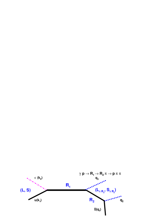
Figure 1: Photoproduction of two mesons due to the cascade of a resonance

The general form of the angular dependent part of the amplitude for such a process is

$$\bar{u}(q_{1})\tilde{N}_{\alpha_{1}\ldots\alpha_{n}}(R_{2}\!\to\!\mu N)F^{\alpha_{1}\ldots\alpha_{n}}_{\beta_{1}\ldots\beta_{n}}(q_{1}+q_{2})$$

$$\tilde{N}^{(j)\beta_{1}\ldots\beta_{n}}_{\gamma_{1}\ldots\gamma_{m}}(R_{1}\!\to\!\mu R_{2})F^{\gamma_{1}\ldots\gamma_{m}}_{\xi_{1}\ldots\xi_{m}}(P)V^{(i)\mu}_{\xi_{1}\ldots\xi_{m}}(R_{1}\!\to\!\gamma N)$$

$$u(k_{1})\varepsilon_{\mu},\qquad\qquad P=q_{1}+q_{2}+q_{3}=k_{1}+k_{2}$$ (153)

The resonance $R_{1}$ with spin $J=m+1/2$ is produced in $\gamma N$ interaction, propagates and then decays into a meson and a baryon resonance $R_{2}$ with spin $J=n+1/2$. Then the resonance $R_{2}$ propagates and decays into the final meson and a nucleon.

In the following the full vertex functions used for the construction of amplitudes are given here for convenience of the reader. One should remember that the $\tilde{N}$ functions are different from $N$-functions by the order of $\gamma$-matrices. For $R\to 0^{-}\!+1/2^{+}$ transitions

$$\tilde{N}^{+}_{\mu_{1}\ldots\mu_{n}}=X^{(n)}_{\mu_{1}\ldots\mu_{n}}\;\;\tilde{N}^{-}_{\mu_{1}\ldots\mu_{n}}=i\gamma_{\nu}\gamma_{5}X^{(n+1)}_{\nu\mu_{1}\ldots\mu_{n}}$$ (154)

holds, while we have

$$\begin{array}[]{ll}\tilde{N}^{(1+)\mu}_{\alpha_{1}\ldots\alpha_{n}}=i\gamma_{\nu}\gamma_{5}X^{(n+2)}_{\mu\nu\alpha_{1}\ldots\alpha_{n}}\;,&\tilde{N}^{(1-)\mu}_{\alpha_{1}\ldots\alpha_{n}}=X^{(n+1)}_{\mu\alpha_{1}\ldots\alpha_{n}}\;,\\ \tilde{N}^{(2+)\mu}_{\alpha_{1}\ldots\alpha_{n}}=i\gamma_{\nu}\gamma_{5}X^{(n)}_{\nu\alpha_{2}\ldots\alpha_{n}}g^{\perp}_{\alpha_{1}\mu}\;,&\tilde{N}^{(2-)\mu}_{\alpha_{1}\ldots\alpha_{n}}=X^{(n-1)}_{\alpha_{2}\ldots\alpha_{n}}g^{\perp}_{\alpha_{1}\mu}\;.\end{array}$$ (157)

(158)

for $R\to 0^{-}\!+3/2^{+}$ transitions, and

$$\begin{array}[]{ll}V^{(1+)\mu}_{\alpha_{1}\ldots\alpha_{n}}=\gamma_{\mu}i\gamma_{5}X^{(n)}_{\alpha_{1}\ldots\alpha_{n}}\;,&V^{(1-)\mu}_{\alpha_{1}\ldots\alpha_{n}}=\gamma_{\xi}\gamma_{\mu}X^{(n+1)}_{\xi\alpha_{1}\ldots\alpha_{n}}\;,\\ V^{(2+)\mu}_{\alpha_{1}\ldots\alpha_{n}}=\gamma_{\nu}i\gamma_{5}X^{(n+2)}_{\mu\nu\alpha_{1}\ldots\alpha_{n}}\;,&V^{(2-)\mu}_{\alpha_{1}\ldots\alpha_{n}}=X^{(n+1)}_{\mu\alpha_{1}\ldots\alpha_{n}}\;,\\ V^{(3+)\mu}_{\alpha_{1}\ldots\alpha_{n}}=\gamma_{\nu}i\gamma_{5}X^{(n+1)}_{\nu\alpha_{1}\ldots\alpha_{n}}g^{\perp}_{\mu\alpha_{n}}\;,&V^{(3-)\mu}_{\alpha_{1}\ldots\alpha_{n}}=X^{(n-1)}_{\alpha_{2}\ldots\alpha_{n}}g^{\perp}_{\alpha_{1}\mu}\;.\end{array}$$ (162)

(163)

for $R\to 1^{-}\!+1/2^{+}$ transitions. Here $n$ is related to the total spin of the resonance by $J=n+1/2$.

7.1 Amplitudes for baryons states decaying into a $1/2$ state and a pion

In this section explicit expressions for the angular dependent part of the amplitudes are given for the case of a baryon produced in a $\gamma^{*}N$ collision. The baryon decays into a pseudoscalar particle and another (intermediate) baryon with spin 1/2 (decaying in turn into meson and nucleon).

7.1.1 The $1/2^{-},\;3/2^{+},\;5/2^{-}\ldots$ states

The amplitude for a ’+’ state ($R_{1}$) produced in a $\gamma^{*}N$ collision in a partial wave $(i)$ decaying into a $0^{-}$ meson and an intermediate $1/2^{+}$ baryon ($R_{2}$) has the form

$$A^{(i)}=\bar{u}(q_{1})\tilde{N}^{-}(q^{\perp}_{12})\;\frac{\hat{q}_{1}\!+\!\hat{q}_{2}\!+\!\sqrt{s_{12}}}{2\sqrt{s_{12}}}\tilde{N}^{+}_{\alpha_{1}\ldots\alpha_{L}}(q^{\perp}_{1})$$

$$F^{\alpha_{1}\ldots\alpha_{L}}_{\beta_{1}\ldots\beta_{L}}(P)V^{(i+)\mu}_{\beta_{1}\ldots\beta_{L}}(k^{\perp})u(k_{1})\varepsilon_{\mu}$$

$$=\bar{u}(q_{1})\;i\hat{q}^{\perp}_{12}\gamma_{5}\;\frac{\hat{q}_{1}\!+\!\hat{q}_{2}\!+\!\sqrt{s_{12}}}{2\sqrt{s_{12}}}\;X^{(L)}_{\alpha_{1}\ldots\alpha_{L}}(q^{\perp}_{1})\frac{\sqrt{s}\!+\!\hat{P}}{2\sqrt{s}}\;$$

$$R^{\alpha_{1}\ldots\alpha_{L}}_{\beta_{1}\ldots\beta_{L}}V^{(i+)\mu}_{\beta_{1}\ldots\beta_{L}}(k^{\perp})u(k_{1})\varepsilon_{\mu}\;,$$ (164)

where the $k_{1}$ and $q_{1}$ are the momenta of the nucleon in the initial and the final state, $k^{\perp}=1/2(k_{1}-k_{2})^{\perp}$ and $q_{1}^{\perp}=1/2(q_{1}+q_{2}-q_{3})^{\perp}$ are their components orthogonal to the total momentum of the first resonance $R_{1}$. Further, $s_{12}=(q_{1}+q_{2})^{2}$ and the factors $1/(2\sqrt{s})$ and $1/(2\sqrt{s_{12}})$ are introduced to suppress the divergency of the numerator of the fermion propagators at large energies. The relative momentum $q_{12}^{\perp}$ is the component of $q_{1}$ and $q_{2}$ orthogonal to the total momentum $q_{1}+q_{2}$. It is given by:

$$q_{12\mu}^{\perp}=\frac{1}{2}(q_{1}-q_{2})_{\nu}\left(g_{\mu\nu}-\frac{(q_{1}+q_{2})_{\mu}(q_{1}+q_{2})_{\nu}}{(q_{1}+q_{2})^{2}}\right)$$ (165)

The vertex functions (154)-(158) are given for the case when the nucleon wave function is placed on the right-hand side of the amplitude. Therefore the order of the $\gamma$-matrices needs to be changed for the meson-nucleon vertices in eq.(153).

If the baryon $R_{2}$ has spin $1/2^{-}$ one has to construct the vertex for decay of ’+’ states into a $0^{-}$ and a $1/2^{-}$ particle. However such operators coincide with the operators for the decay of ’-’ states into a $0^{-}+1/2^{+}$ system. Therefore

$$A^{(i)}=\bar{u}(q_{1})\tilde{N}^{+}(q^{\perp}_{12})\;\frac{\hat{q}_{1}\!+\!\hat{q}_{2}\!+\!\sqrt{s_{12}}}{2\sqrt{s_{12}}}\tilde{N}^{-}_{\alpha_{1}\ldots\alpha_{L}}(q^{\perp}_{1})$$

$$F^{\alpha_{1}\ldots\alpha_{L}}_{\beta_{1}\ldots\beta_{L}}(P)V^{(i+)\mu}_{\beta_{1}\ldots\beta_{L}}(k^{\perp})u(k_{1})\varepsilon_{\mu}=$$

$$\bar{u}(q_{1})\;\frac{\hat{q}_{1}\!+\!\hat{q}_{2}\!+\!\sqrt{s_{12}}}{2\sqrt{s_{12}}}i\gamma_{\nu}\gamma_{5}X^{(L+1)}_{\nu\alpha_{1}\ldots\alpha_{L}}(q^{\perp}_{1})$$

$$F^{\alpha_{1}\ldots\alpha_{L}}_{\beta_{1}\ldots\beta_{L}}(P)V^{(i+)\mu}_{\beta_{1}\ldots\beta_{L}}(k^{\perp})u(k_{1})\varepsilon_{\mu}\;.$$ (166)

In case of the photoproduction with real photons, the $V^{(2+)\mu}_{\beta_{1}\ldots\beta_{L}}$ vertex is reduced to $V^{(1+)\mu}_{\beta_{1}\ldots\beta_{L}}$, and can be omitted.

7.1.2 The $1/2^{+},\;3/2^{-},\;5/2^{+}\ldots$ states

If a ’-’ state is produced in a $\gamma^{*}N$ interaction and then decays into a pseudoscalar pion and $1/2^{+}$ baryon the amplitude has the structure

$$A^{(i)}\!=\bar{u}(q_{1})\tilde{N}^{-}(q^{\perp}_{12})\;\frac{\hat{q}_{1}\!+\!\hat{q}_{2}\!+\!\sqrt{s_{12}}}{2\sqrt{s_{12}}}\tilde{N}^{-}_{\alpha_{1}\ldots\alpha_{L-1}}(q^{\perp}_{1})$$

$$F^{\alpha_{1}\ldots\alpha_{L-1}}_{\beta_{1}\ldots\beta_{L-1}}(P)V^{(i-)\mu}_{\beta_{1}\ldots\beta_{L-1}}(k^{\perp})u(k_{1})\varepsilon_{\mu}=$$

$$\bar{u}(q_{1})\;i\hat{q}^{\perp}_{12}\gamma_{5}\;\frac{\hat{q}_{1}\!+\!\hat{q}_{2}\!+\!\sqrt{s_{12}}}{2\sqrt{s_{12}}}i\gamma_{\nu}\gamma_{5}X^{(L)}_{\nu\alpha_{1}\ldots\alpha_{L-1}}(q^{\perp}_{1})$$

$$F^{\alpha_{1}\ldots\alpha_{L-1}}_{\beta_{1}\ldots\beta_{L-1}}(P)V^{(i-)\mu}_{\beta_{1}\ldots\beta_{L-1}}(k^{\perp})u(k_{1})\varepsilon_{\mu}\;.$$ (167)

If the intermediate baryon has spin $1/2^{-}$ then:

$$A^{(i)}\!=\bar{u}(q_{1})\tilde{N}^{+}(q^{\perp}_{12})\;\frac{\hat{q}_{1}\!+\!\hat{q}_{2}\!+\!\sqrt{s_{12}}}{2\sqrt{s_{12}}}\tilde{N}^{+}_{\alpha_{1}\ldots\alpha_{L-1}}(q^{\perp}_{1})$$

$$F^{\alpha_{1}\ldots\alpha_{L-1}}_{\beta_{1}\ldots\beta_{L-1}}(P)V^{(i-)\mu}_{\beta_{1}\ldots\beta_{L-1}}(k^{\perp})u(k_{1})\varepsilon_{\mu}=$$

$$\bar{u}(q_{1})\;\frac{\hat{q}_{1}\!+\!\hat{q}_{2}\!+\!\sqrt{s_{12}}}{2\sqrt{s_{12}}}X^{(L)}_{\alpha_{1}\ldots\alpha_{L}}(q^{\perp}_{1})$$

$$F^{\alpha_{1}\ldots\alpha_{L-1}}_{\beta_{1}\ldots\beta_{L-1}}(P)V^{(i-)\mu}_{\beta_{1}\ldots\beta_{L-1}}(k^{\perp})u(k_{1})\varepsilon_{\mu}\;.$$ (168)

For photoproduction with real photons only amplitudes with $V^{(1-)}$ and $V^{(3-)}$ vertex functions should be taken into account.

7.2 Photoproduction amplitudes for baryon states decaying into a $3/2$ state and a pseudoscalar meson

Experimentally important is photoproduction of resonances decaying into $\Delta(1232)\pi$ followed by a $\Delta(1232)$ decay into a nucleon and a pion.

7.2.1 The $1/2^{-},\;3/2^{+},\;5/2^{-}\ldots$ states decaying into a meson with spin $0$ and a baryon with spin $3/2$

The ’+’ states produced in a $\gamma^{*}N$ collision can decay into a pseudoscalar meson and an intermediate baryon with spin $3/2^{+}$ in two partial waves. The amplitude depends on indices $(ij)$ where index $(i)$ is related, as before, to the partial wave in the $\gamma N$ channel while index $(j)$ is related to the partial wave in the decay of the resonance into the spin $0$ meson and the $3/2$ resonance $R_{2}$.

$$A^{(ij)}=\bar{u}(q_{1})\;\tilde{N}^{+}_{\delta}(q^{\perp}_{12})F^{\delta}_{\nu}(q_{1}+q_{2})\;\tilde{N}^{(j+)\nu}_{\alpha_{1}\ldots\alpha_{L}}(q^{\perp}_{1})$$

$$F^{\alpha_{1}\ldots\alpha_{L}}_{\beta_{1}\ldots\beta_{L}}(P)V^{(i+)\mu}_{\beta_{1}\ldots\beta_{L}}(k^{\perp})u(k_{1})\varepsilon_{\mu}\;.$$ (169)

If the intermediate baryon $R_{2}$ has $J^{P}=3/2^{-}$, the structure of the amplitude structure is

$$A^{(ij)}=\bar{u}(q_{1})\;\tilde{N}^{-}_{\delta}(q^{\perp}_{12})F^{\delta}_{\nu}(q_{1}+q_{2})\;\tilde{N}^{(j-)\nu}_{\alpha_{1}\ldots\alpha_{L}}(q^{\perp}_{1})$$

$$F^{\alpha_{1}\ldots\alpha_{L}}_{\beta_{1}\ldots\beta_{L}}(P)V^{(i+)\mu}_{\beta_{1}\ldots\beta_{L}}(k^{\perp})u(k_{1})\varepsilon_{\mu}\;.$$ (170)

7.2.2 The $1/2^{+},\;3/2^{-},\;5/2^{+}\ldots$ states decaying into a $0^{-}$ meson and a $3/2^{+}$ baryon

The amplitudes for ’-’ states decaying into $0^{-}$ meson and $3/2^{+}$ intermediate baryon are

$$A^{(ij)}=\bar{u}(q_{1})\;\tilde{N}^{+}_{\delta}(q^{\perp}_{12})\;F^{\delta}_{\nu}(q_{1}+q_{2})\;\tilde{N}^{(j-)\nu}_{\alpha_{1}\ldots\alpha_{L-1}}(q^{\perp}_{1})$$

$$F^{\alpha_{1}\ldots\alpha_{L-1}}_{\beta_{1}\ldots\beta_{L-1}}(P)V^{(i-)\mu}_{\beta_{1}\ldots\beta_{L-1}}(k^{\perp})u(k_{1})\varepsilon_{\mu}\;.$$ (171)

and if the intermediate baryon $R_{2}$ has the quantum numbers $3/2^{-}$

$$A^{(ij)}=\bar{u}(q_{1})\;\tilde{N}^{-}_{\delta}(q^{\perp}_{12})\;F^{\delta}_{\nu}(q_{1}+q_{2})\;\tilde{N}^{(j+)\nu}_{\alpha_{1}\ldots\alpha_{L-1}}(q^{\perp}_{1})$$

$$F^{\alpha_{1}\ldots\alpha_{L-1}}_{\beta_{1}\ldots\beta_{L-1}}(P)V^{(i-)\mu}_{\beta_{1}\ldots\beta_{L-1}}(k^{\perp})u(k_{1})\varepsilon_{\mu}\;.$$ (172)

8 t- and u-channel exchange amplitudes

Meson exchange in the t-channel plays an important role in both, in photoproduction and in pion induced reactions. Especially at large energies this mechanism often dominates. In the resonance region we expect that production of baryon resonances in the s-channel dominates the interaction, at least when neutral mesons are produced. Nevertheless the t- and u-channel exchanges must be taken into account carefully.

The most straight forward parameterization of particle exchange amplitudes is the exchange of Regge trajectories. For construction of a cross-symmetrical amplitude it is convenient to use the variable

$$\nu=\frac{1}{2}(s-u).$$

The amplitude for t-channel exchange can be written as

$$A=g_{1}(t)g_{2}(t)\frac{1+\xi exp(-i\pi\alpha(t))}{\sin(\pi\alpha(t))}\left(\frac{\nu}{\nu_{0}}\right)^{\alpha(t)}\;.$$ (173)

Here $g_{i}$ are vertex functions, $\alpha(t)$ is the function which describes the trajectory, $\nu_{0}$ is a normalization factor (which can be taken to be 1) and $\xi$ is the signature of the trajectory. The Pomeron, $f_{0}$ and $\pi$ exchanges have a positive signature while $\rho$, $\omega$ and $a_{1}$ exchanges have a negative one.

Accordingly, the Reggeon propagators can be written as

$$R(+,\nu,t)=\frac{e^{-i\frac{\pi}{2}\alpha(t)}}{\sin(\frac{\pi}{2}\alpha(t))}\left(\frac{\nu}{\nu_{0}}\right)^{\alpha(t)}\;,$$

$$R(-,\nu,t)=\frac{ie^{-i\frac{\pi}{2}\alpha(t)}}{\cos(\frac{\pi}{2}\alpha(t))}\left(\frac{\nu}{\nu_{0}}\right)^{\alpha(t)}\;.$$ (174)

where ’+’ and ’-’ indicate the signature of the Regge-trajectories. To eliminate the poles at $t<0$ additional $\Gamma$-functions are introduced in (174). If the Pomeron trajectory is taken as $1.0+0.15t$ pom_slope , negative $t$ poles are at $\alpha=0,-2,-4,\ldots$ and therefore

$$\sin\left(\frac{\pi}{2}\alpha(t)\right)\to\sin\left(\frac{\pi}{2}\alpha(t)\right)\;\Gamma\left(\frac{\alpha(t)}{2}\right)\;.$$ (175)

For the pion trajectory $\alpha(t)=-0.014+0.72t$ pom_slope , and the negative poles are at $\alpha=-2,-4,\ldots$. Regularization must be taken as

$$\sin\left(\frac{\pi}{2}\alpha(t)\right)\to\sin\left(\frac{\pi}{2}\alpha(t)\right)\;\Gamma\left(\frac{\alpha(t)}{2}+1\right)\;.$$ (176)

For $\rho$, $\omega$ and $a_{1}$ exchanges the negative poles start from $a=-1$ and therefore

$$\cos\left(\frac{\pi}{2}\alpha(t)\right)\to\cos\left(\frac{\pi}{2}\alpha(t)\right)\;\Gamma\left(\frac{\alpha(t)}{2}+\frac{1}{2}\right)\,.$$ (177)

8.1 Single meson photoproduction due to $\rho$ and $\omega$ exchange

In the following, the 4-vectors of the initial photon and proton are denoted as $k_{1}$ and $k_{2}$ and 4-vectors of the final state nucleon (e.g. proton) and the meson (e.g. pion) as $q_{1}$ and $q_{2}$ respectively (see Fig. 2). The photon couples to the $\pi\rho(770)$ system in a P-wave, and the corresponding amplitude for upper vertex is

$$A_{upper}=\varepsilon_{\mu}\rho_{\alpha}\epsilon_{\mu\alpha\beta\gamma}\;q_{2\beta}\;k_{2\gamma}\;,$$ (178)

where $\rho_{\alpha}$ is the polarization vector of $\rho$-meson.

Figure 2: The t-channel exchange diagram for single meson photoproduction

Another vertex in this diagram describes the transition of the proton and the $\rho$-meson into the final proton. Such a transition has the same vertex structure as the transition $\gamma^{*}N$ to a nucleon at the lower vertex:

$$A_{lower}^{(i-)}=\bar{u}(q_{1})V^{(i-)\mu}(k_{1}^{\perp})u(k_{1})\rho_{\mu}\;,\qquad\qquad i=1,2$$

$$k_{1\mu}^{\perp}=k_{1\nu}\Big{(}g_{\mu\nu}-\frac{q_{1\mu}q_{1\nu}}{q_{1}^{2}}\Big{)}=\frac{1}{2}(k_{1}-k_{t})_{\nu}\Big{(}g_{\mu\nu}-\frac{q_{1\mu}q_{1\nu}}{q_{1}^{2}}\Big{)}\;.$$

Here $k_{t}=k_{2}-q_{2}=q_{1}-k_{1}$ is the $\rho$-meson momentum. Summing over its polarizations yields

$$\sum\limits_{polarization}\rho_{\alpha}\rho_{\beta}=g_{\alpha\beta}-\frac{k_{t\alpha}k_{t\beta}}{k_{t}^{2}}\;,$$ (180)

we obtain the following expression for the amplitude:

$$A^{i-}=\varepsilon_{\mu}\epsilon_{\mu\alpha\beta\gamma}\;q_{2\beta}\;k_{2\gamma}\bar{u}(q_{1})V^{(i-)\alpha}(k_{1}^{\perp})u(k_{1})\;,\;\;i=1,2$$

(181)

The same amplitude structure corresponds also to $\omega$- exchange.

8.2 Double meson photoproduction due to $\rho$ and $\omega$ exchange

Let us consider photoproduction of two meson (e.g. pions) due to $\rho$ exchange in t-channel with a $1/2$ resonance in the intermediate state (see Fig. 3).

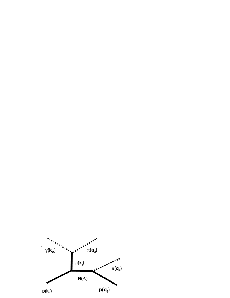
Figure 3: The t-channel exchange diagram for double meson photoproduction reactions

In this case we should add to eq.(181) the $1/2$ propagator and the vertex for decay of this resonance into final meson and nucleon:

$$A^{i\pm}=\varepsilon_{\mu}\epsilon_{\mu\alpha\beta\gamma}\;q_{3\beta}\;k_{2\gamma}\bar{u}(q_{1})\tilde{N}^{\pm}(q^{\perp}_{12})\;\frac{\hat{q}_{1}\!+\!\hat{q}_{2}\!+\!\sqrt{s_{12}}}{2\sqrt{s_{12}}}$$

$$V^{(i\pm)\alpha}(k_{1}^{\perp})u(k_{1})\;,\quad\quad i=1,2\;$$ (182)

with    $k_{1\mu}^{\perp}=k_{1\nu}\big{(}g_{\mu\nu}-(q_{1}+q_{2})_{\mu}(q_{1}+q_{2})_{\nu}/s_{12}\big{)}$.
The definition of $q_{12}^{\perp}$ is given in (165). The ’-’ amplitude corresponds to production of a $1/2^{+}$ intermediate state while the ’+’ amplitude corresponds to production of a $1/2^{-}$ intermediate state.

Two-meson photoproduction due to $\rho$ exchange in t-channel with a $3/2$ resonance in the intermediate state can be easily obtained following the procedure given above. In

$$A^{i\pm}=\varepsilon_{\mu}\epsilon_{\mu\alpha\beta\gamma}\;q_{3\beta}\;k_{2\gamma}\bar{u}(q_{1})\tilde{N}^{\pm}_{\xi}(q^{\perp}_{12})\;$$

$$F^{\xi}_{\chi}(q_{1}+q_{2})V^{(i\pm)\alpha}_{\chi}(k_{1}^{\perp})u(k_{1})\qquad i=1,2,3$$ (183)

the ’-’ amplitude corresponds to a $3/2^{-}$ intermediate state and ’+’ amplitude to $3/2^{+}$ intermediate state.

The examples of other $t$-channel and u-channel exchange amplitudes exchange amplitudes used in the analysis of the single and double meson photoproduction are given in Appendix D.

9 The cross section for photoproduction processes

The differential cross section for production of two or more particles has the form:

$$d\sigma=\frac{(2\pi)^{4}|A|^{2}}{4\sqrt{(k_{1}k_{2})^{2}-m_{1}^{2}m_{2}^{2}}}d\Phi_{n}(k_{1}+k_{2},q_{1},\ldots,q_{n})\;,$$

where $k_{1}$ and $k_{2}$ are momenta of the initial particles (nucleon and $\gamma$ in the case of photoproduction) and $q_{i}$ are momenta of final state particles. The $d\Phi_{n}(k_{1}+k_{2},q_{1},\ldots,q_{n})$ is the element of the n-body phase volume given by

$$d\Phi_{n}(k_{1}+k_{2},q_{1},\ldots,q_{n}) = \delta^{4}(k_{1}+k_{2}-\sum\limits_{i=1}^{n}q_{i})$$ (185)

$$\prod\limits_{i=1}^{n}\frac{d^{3}q_{i}}{(2\pi)^{3}2q_{0i}}\;.$$

The photoproduction amplitude can be written as

$$A=\varepsilon_{\mu}\bar{u}_{i}A_{\mu}u_{f}\;,$$ (186)

where $\varepsilon_{\mu}$ is the $\gamma$ polarization vector and $\bar{u}_{i}$ and $u_{f}$ are the bispinors of the initial and final state nucleon. When the $\gamma$ and nucleon polarization are not measured the amplitude squared is equal to

$$|A|^{2}=\frac{1}{4}\sum\limits_{\alpha jk}A\;A^{*}=\frac{1}{4}\sum\limits_{\alpha jk}\varepsilon^{\alpha}_{\mu}\varepsilon^{\alpha}_{\nu}\bar{u}^{j}_{i}A_{\mu}u^{k}_{f}\bar{u}^{k}_{f}A^{tr}_{\nu}u^{j}_{i}\;,\;$$ (187)

where one averages over the polarization of the initial and sums over the polarization of the final state particles. $A^{tr}$ is the hermitian conjugate amplitude.

For the unpolarized real photons:

$$-\sum\limits_{\alpha}\varepsilon^{\alpha}_{\mu}\varepsilon^{\alpha}_{\nu}=g_{\mu\nu}^{\perp\perp}=g_{\mu\nu}-\frac{P_{\mu}P_{\nu}}{P^{2}}-\frac{k^{\perp}_{\mu}k^{\perp}_{\nu}}{k_{\perp}^{2}}$$ (188)

with $P=k_{1}+k_{2}$ and

$$k^{\perp}_{\mu}=\frac{1}{2}(k_{1}-k_{2})_{\nu}g^{\perp}_{\mu\nu}=\frac{1}{2}(k_{1}-k_{2})_{\nu}\left(g^{\perp}_{\mu\nu}-\frac{P_{\mu}P_{\nu}}{P^{2}}\right)$$

Let us remind that in the c.m.s. with the momentum of $\gamma$ being parallel to the z-axis:

$$g^{\perp\perp}_{\mu\nu}\qquad=\qquad\left(\begin{array}[]{cccc}0&0&0&0\\ 0&-1&0&0\\ 0&0&-1&0\\ 0&0&0&0\end{array}\right)\;.$$ (193)

The bispinors of fermions with momentum $k_{1}$ summed over polarization are convoluted (taking into account normalization (40)) and yield

$$\sum\limits_{j}u^{j}(k_{1})\bar{u}^{j}(k_{1})=m+\hat{k}_{1}$$ (194)

and therefore

$$|A|^{2}=\frac{1}{4}g_{\mu\nu}^{\perp\perp}Tr\left[(m+\hat{k}_{1})A_{\mu}(m+\hat{q}_{1})A^{tr}_{\nu}\right]\;.$$ (195)

In case of a polarised target the density matrix of the fermion propagator $(m+\hat{k}_{1})$ must be changed to the polarization density matrix:

$$m+\hat{k}_{1}\to(m+\hat{k}_{1})(1+\gamma_{5}\hat{S}_{T})\;,$$ (196)

where the 4-vector $S_{T}$ is the polarization vector of the target baryon ($S^{2}_{T}=-1$, $(k_{1}S_{T})=0$). If the polarisation of final baryon is measured the density matrix of the propagator $(m+\hat{q}_{1})$ is substituted by:

$$m+\hat{q}_{1}\to(m+\hat{q}_{1})(1+\gamma_{5}\hat{S}_{R})\;,$$ (197)

where the 4-vector $S_{R}$ is the polarization vector of the final baryon ($S^{2}_{R}=-1$, $(q_{1}S_{R})=0$).

When a $\gamma$ is linearly polarised along the x-axis the polarization vector is: $\varepsilon_{\mu}=(0,1,0,0)$ and we do not need to average over two polarizations. Then one has to change (195) by substituting

$$\frac{1}{2}g^{\perp\perp}_{\mu\nu}\qquad\to\qquad\left(\begin{array}[]{cccc}0&0&0&0\\ 0&-1&0&0\\ 0&0&0&0\\ 0&0&0&0\end{array}\right)$$ (202)

If one has a circular polarised beam

$$\frac{1}{2}g^{\perp\perp}_{\mu\nu}\qquad\to\qquad\frac{1}{2}\left(\begin{array}[]{cccc}0&0&0&0\\ 0&-1&-i&0\\ 0&i&-1&0\\ 0&0&0&0\end{array}\right)$$ (207)

10 Conclusion

In the present paper the operator expansion approach has been developed for the construction of amplitudes for pion- and photon-induced reactions. The method is relativistically invariant and can be easily applied to the construction of amplitudes with multi-body final states. For production of pseudoscalar mesons the identity of our amplitudes to the well known CGLN amplitudes is explicitly shown. The formulas are given explicitly in the form used by the Crystal Barrel at ELSA collaboration in the analysis of single and double meson photoproduction.

Appendices

A   Properties of Legendre polynomials

The recurrent expression for Legendre polynomials is given by

$$P_{L}(z)\ =\ \frac{2L-1}{L}\ z\ P_{L-1}(z)-\frac{L-1}{L}\ P_{L-2}(z)\;.$$ (208)

The first and second derivative of the Legendre polynomials can be expressed as

$$P^{\prime}_{L}(z)\ =\ L\frac{P_{L-1}(z)-z\ P_{L}(z)}{1-z^{2}}\ =\ (L+1)\frac{z\ P_{L}-P_{L+1}}{1-z^{2}}\ \;,$$

$$P^{\prime\prime}_{L}(z) = \frac{2z\ P^{\prime}_{L}(z)-L(L+1)\ P_{L}(z)}{1-z^{2}}\$$ (210)

$$= \ \frac{2P^{\prime}_{L+1}(z)-(L+1)(L+2)\ P_{L}(z)}{1-z^{2}}\;.$$

Some other useful expressions given here for convenience are:

$$P^{\prime}_{L-1}=P^{\prime}_{L}\ z-L\ P_{L},\;\;P^{\prime}_{L+1}=P^{\prime}_{L}\ z+(L+1)\ P_{L}\;,$$

$$P^{\prime}_{L+1}-P^{\prime}_{L-1}\ =\ (2L+1)P_{L}\;,$$

$$P^{\prime\prime}_{L+1}-P^{\prime\prime}_{L-1}\ =\ (2L+1)P^{\prime}_{L}\;.$$

B   Properties of angular momentum operators

In the following we list useful properties of angular momentum operators.

$$X^{(n+1)}_{\mu\alpha_{1}\ldots\alpha_{n}}(q_{\perp})X^{(n)}_{\alpha_{1}\ldots\alpha_{n}}(k_{\perp})=$$ (211)

$$\frac{\alpha_{n}}{n+1}(\sqrt{k_{\perp}^{2}})^{n}(\sqrt{q_{\perp}^{2}})^{n+1}\biggl{[}-\frac{k_{1\mu}}{\sqrt{k_{\perp}^{2}}}P^{\prime}_{n}+\frac{q_{1\mu}}{\sqrt{q_{\perp}^{2}}}P^{\prime}_{n+1}\biggl{]}\;,$$

$$X^{(n)}_{\mu\alpha_{2}\ldots\alpha_{n}}(q_{\perp})X^{(n)}_{\nu\alpha_{2}\ldots\alpha_{n}}(k_{\perp})=$$

$$\frac{\alpha_{n-1}}{n^{2}}(\sqrt{k_{\perp}^{2}})^{n}(\sqrt{q_{\perp}^{2}})^{n}\biggl{[}g^{\perp}_{\mu\nu}P^{\prime}_{n-1}-\biggl{(}\frac{q_{\mu}^{\perp}q_{\nu}^{\perp}}{q_{\perp}^{2}}+\frac{k_{\mu}^{\perp}k_{\nu}^{\perp}}{k_{\perp}^{2}}\biggl{)}P^{\prime\prime}_{n}+$$

$$\frac{1}{2}\biggl{(}\frac{q_{\mu}^{\perp}k_{\nu}^{\perp}+k_{\mu}^{\perp}q_{\nu}^{\perp}}{\sqrt{k_{\perp}^{2}}\sqrt{q_{\perp}^{2}}}\biggl{)}(P^{\prime}_{n}+2zP^{\prime\prime}_{n})+$$ (212)

$$\frac{2n-1}{2}\biggl{(}\frac{q_{\mu}^{\perp}k_{\nu}^{\perp}-k_{\mu}^{\perp}q_{\nu}^{\perp}}{\sqrt{k_{\perp}^{2}}\sqrt{q_{\perp}^{2}}}\biggl{)}P^{\prime}_{n}\biggl{]}\;,$$

$$X^{(n+2)}_{\mu\nu\alpha_{1}\ldots\alpha_{n}}(q_{\perp})X^{(n)}_{\alpha_{1}\ldots\alpha_{n}}(k_{\perp})=$$

$$\frac{2}{3}\frac{\alpha_{n}}{(n+1)(n+2)}(\sqrt{k_{\perp}^{2}})^{n}(\sqrt{q_{\perp}^{2}})^{n+2}\biggl{(}\frac{X^{(2)}_{\mu\nu}(q_{\perp})}{q_{\perp}^{2}}P^{\prime\prime}_{n+2}+$$

$$\frac{X^{(2)}_{\mu\nu}(k_{\perp})}{k_{\perp}^{2}}P^{\prime\prime}_{n}-\frac{3}{2}\frac{k_{\mu}^{\perp}q_{\nu}^{\perp}+k_{\nu}^{\perp}q_{\mu}^{\perp}-\frac{2}{3}g_{\mu\nu}^{\perp}(k^{\perp}q^{\perp})}{\sqrt{k_{\perp}^{2}}\sqrt{q_{\perp}^{2}}}P^{\prime\prime}_{n+1}\biggl{)}\;,$$

$$X^{(n)}_{\alpha\gamma_{2}\ldots\gamma_{n}}(q_{\perp})O_{\mu\beta_{2}\ldots\beta_{n}}^{\tau\gamma_{2}\ldots\gamma_{n}}X^{(n)}_{\xi\beta_{2}\ldots\beta_{n}}(k_{\perp})=$$

$$X^{(n)}_{\alpha\gamma_{2}\ldots\gamma_{n}}(q_{\perp})\frac{g_{\tau\mu}}{n}X^{(n)}_{\xi\gamma_{2}\ldots\gamma_{n}}(k_{\perp})+$$

$$+\frac{n-1}{n}X^{n}_{\alpha\mu\gamma_{3}\ldots\gamma_{n}}(q_{\perp})X^{(n)}_{\xi\tau\gamma_{3}\ldots\gamma_{n}}(k_{\perp})-$$

$$\frac{2(n-1)}{n(2n-1)}X^{(n)}_{\alpha\tau\gamma_{3}\ldots\gamma_{n}}(q_{\perp})X^{(n)}_{\xi\mu\gamma_{3}\ldots\gamma_{n}}(k_{\perp})\;.$$ (214)

C   Blatt-Weisskopf formfactors

If a resonance with radius $r$ decays into two particle with (squared) momentum $k^{2}$:

$$k^{2}=\frac{(s-(m_{1}+m_{2})^{2})(s-(m_{1}-m_{2}))^{2}}{4s},$$ (215)

where $s$ is total energy and $m_{1}$ and $m_{2}$ are masses of the final particles, then the first few expressions for formfactors $F(L,k^{2},r)$ are

$$F(0,k^{2},r) = 1\;,$$

$$F(1,k^{2},r) = \frac{\sqrt{(x+1)}}{r}\;,$$

$$F(2,k^{2},r) = \frac{\sqrt{(x^{2}+3x+9)}}{r^{2}}\;,$$ (216)

$$F(3,k^{2},r) = \frac{\sqrt{(x^{3}+6x^{2}+45x+225)}}{r^{3}}\;,$$

$$F(4,k^{2},r) = \frac{\sqrt{x^{4}+10x^{3}+135x^{2}+1575x+11025}}{r^{4}}\;,$$

where $x=k^{2}r^{2}$. Remember that
$r(GeV^{-1})=r(fm)/(0.1973(fmGeV))$.

D   Structure of amplitudes for t-channel and u-channel exchanges

D1   t-channel amplitudes

For the photoproduction of a single neutral pion, $\rho$ and $\omega$ exchanges play a significant role. The exchange of a $\pi^{0}$ is forbidden since the photon does not couple to a neutral pion. When charged pions are produced the pion exchange diagram can play an important role. The upper vertex function for pion exchange is

$$A_{upper} = \varepsilon_{\mu}\frac{1}{2}(k_{2}+k_{t})_{\nu}\Big{(}g_{\mu\nu}-\frac{q_{2\mu}q_{2\nu}}{m_{\pi}^{2}}\Big{)}=$$ (217)

$$\varepsilon_{\mu}k_{t\nu}\Big{(}g_{\mu\nu}-\frac{q_{2\mu}q_{2\nu}}{m_{\pi}^{2}}\Big{)}\;.$$

The lower vertex function is described by a $N\to\pi N$ transition. Thus

$$A=\varepsilon_{\mu}k_{t\nu}\Big{(}g_{\mu\nu}-\frac{q_{2\mu}q_{2\nu}}{m_{\pi}^{2}}\Big{)}\bar{u}(q_{1})N^{-}(k_{1}^{\perp})u(k_{1})\;.$$ (218)

Remember that for single meson production

$$k_{1\mu}^{\perp}=\frac{1}{2}(k_{1}-k_{t})_{\nu}\Big{(}g_{\mu\nu}-\frac{q_{1\mu}q_{1\nu}}{q_{1}^{2}}\Big{)}=k_{1\nu}\Big{(}g_{\mu\nu}-\frac{q_{1\mu}q_{1\nu}}{q_{1}^{2}}\Big{)}\;.$$

(219)

This expression can be easily extended to the case of double meson photoproduction. If the intermediate baryon has spin $1/2$ one obtains

$$A^{\pm} = \varepsilon_{\mu}k_{t\nu}\Big{(}g_{\mu\nu}-\frac{q_{2\mu}q_{2\nu}}{m_{\pi}^{2}}\Big{)}$$

$$\bar{u}(q_{1})\tilde{N}^{\pm}(q^{\perp}_{12})\;\frac{\hat{q}_{1}\!+\!\hat{q}_{2}\!+\!\sqrt{s_{12}}}{2\sqrt{s_{12}}}N^{\pm}(k_{1}^{\perp})u(k_{1})\;.$$

Here the ’-’ amplitude corresponds to a $1/2^{+}$ intermediate state, the ’+’ to a $1/2^{-}$ state,

$$k_{1\mu}^{\perp}=k_{1\nu}\big{(}g_{\mu\nu}-(q_{1}+q_{2})_{\mu}(q_{1}+q_{2})_{\nu}/s_{12}\big{)}\;,$$ (221)

the definition of $q_{12}^{\perp}$ is given in eqn.(165) and the notation of momenta is shown in Fig. 3.

For an intermediate resonance with spin $J=L\pm 1/2$ the amplitude structure reads

$$A^{\pm} = \varepsilon_{\mu}k_{t\nu}\Big{(}g_{\mu\nu}-\frac{q_{2\mu}q_{2\nu}}{m_{\pi}^{2}}\Big{)}\bar{u}(q_{1})\tilde{N}^{\pm}_{\alpha_{1}\alpha_{2}\ldots\alpha_{n}}(q^{\perp}_{12})\;$$ (222)

$$F^{\alpha_{1}\alpha_{2}\ldots\alpha_{L}}_{\beta_{1}\beta_{2}\ldots\beta_{L}}(q_{1}+q_{2})N^{\pm}_{\beta_{1}\beta_{2}\ldots\beta_{L}}(k_{1}^{\perp})u(k_{1})\;.$$

The upper vertex for $\rho$-meson production due to pion exchange has the following structure

$$A_{upper} = \varepsilon_{\mu}\epsilon_{\mu\alpha\beta\gamma}\;\frac{1}{2}(q_{3}-q_{2})_{\alpha}q_{2\beta}\;k_{2\gamma}=$$ (223)

$$\varepsilon_{\mu}\epsilon_{\mu\alpha\beta\gamma}\;q_{3\alpha}q_{2\beta}\;k_{2\gamma}\;,$$

while the lower vertex has the same structure as the $\pi N$ scattering amplitude. Therefore

$$A=\varepsilon_{\mu}\epsilon_{\mu\alpha\beta\gamma}\;q_{3\alpha}q_{2\beta}\;k_{2\gamma}\;\bar{u}(q_{1})N^{-}(k_{1}^{\perp})u(k_{1})\;.$$ (224)

Here $k_{1}^{\perp}$ is given by eq.(219).

The $\rho$ meson can also be produced by Pomeron or $f_{0}$ exchange. The upper vertex for such a case is $\varepsilon_{\mu}\frac{1}{2}(q_{3}-q_{2})_{\mu}$ and the amplitude is equal to

$$A=\varepsilon_{\mu}\frac{1}{2}(q_{3}-q_{2})_{\mu}\bar{u}(q_{1})N^{+}(k_{1}^{\perp})u(k_{1})\;.$$ (225)

The next amplitude which we consider is the $f_{0}$ production due to $\rho$ (or $\omega$) t-channel exchange. Such an amplitude has the structure:

$$A^{i-}=\varepsilon_{\mu}\Big{(}g_{\mu\nu}-\frac{k_{t\mu}k_{t\nu}}{k^{2}_{t}}\Big{)}\bar{u}(q_{1})V^{(i-)}_{\nu}(k_{1}^{\perp})u(k_{1})\;\;i=1,2$$

D2   u-channel amplitudes

Figure 4: The u-channel exchange diagram for photoproduction of single mesons

Apart from meson exchange amplitudes (which we define as t-channel exchanges), mesons can be produced from baryon exchange in the u-channel. An example of such a diagram is given in Fig. 4. For nucleon exchange, the vertex for meson production (the lower vertex) is defined by

$$\bar{u}(k_{u})N^{-}(q_{2}^{\perp})u(k_{1})\;,\qquad\qquad k_{u}=k_{1}-q_{2}.$$ (227)

Here the $N^{-}$ vertex describes the production of a pseudoscalar meson. Further,

$$q_{2\mu}^{\perp} = \left(g_{\mu\nu}-\frac{k_{1\mu}k_{1\nu}}{m_{p}^{2}}\right)\frac{1}{2}(q_{2}-k_{u})_{\nu}=$$ (228)

$$\left(g_{\mu\nu}-\frac{k_{1\mu}k_{1\nu}}{m_{p}^{2}}\right)q_{2\nu}.$$

Figure 5: A u-channel exchange diagram for production of a baryon resonance in photoproduction of two mesons

If the reaction is induced by a meson the upper vertex has the same structure

$$\bar{u}(q_{1})N^{-}(k_{2}^{\perp})u(k_{u})\;,$$ (229)

where

$$k_{2\mu}^{\perp}=\left(g_{\mu\nu}-\frac{q_{1\mu}q_{1\nu}}{m_{p}^{2}}\right)\frac{1}{2}(k_{2}-k_{u})_{\nu}=\left(g_{\mu\nu}-\frac{q_{1\mu}q_{1\nu}}{m_{p}^{2}}\right)k_{2\nu}$$

The angular dependent part of the amplitude for the nucleon exchange diagram is

$$A=\bar{u}(q_{1})N^{-}(k_{2}^{\perp})\frac{m_{p}+\hat{k}_{u}}{m_{p}^{2}-k_{u}^{2}}N^{-}(q_{2}^{\perp})u(k_{1})\;.$$ (230)

In the case of photoproduction the upper vertex is defined by $V^{(i-)}_{\mu}$:

$$A^{i}=\varepsilon_{\mu}\bar{u}(q_{1})V^{(i-)}(k_{2}^{\perp})\frac{m_{p}+\hat{k}_{u}}{m_{p}^{2}-k_{u}^{2}}N^{-}(q_{2}^{\perp})u(k_{1}),\;\;i=1,2$$

(231)

The production of $0^{++}$ states in double meson production can be obtained from eqs.(230,231) by replacing $N^{-}(q_{2}^{\perp})$ by $N^{+}(q_{2}^{\perp})$.

In the case when a baryon resonance with $J=L\pm 1/2$ is produced in the intermediate state (see Fig. 5) the amplitude for meson induced reaction has the structure

$$A=\bar{u}(q_{1})N^{\pm}_{\alpha_{1}\alpha_{2}\ldots\alpha_{L}}(q_{12}^{\perp})F^{\alpha_{1}\alpha_{2}\ldots\alpha_{L}}_{\beta_{1}\beta_{2}\ldots\beta_{L}}(q_{1}+q_{2})\;,$$

$$N^{\pm}_{\beta_{1}\beta_{2}\ldots\beta_{L}}(k_{2}^{\perp})\frac{m_{p}+\hat{k}_{u}}{m_{p}^{2}-k_{u}^{2}}N^{-}(q_{3}^{\perp})u(k_{1})$$ (232)

and for $\gamma^{*}$ induced reactions

$$A^{i\pm}=\bar{u}(q_{1})V^{(i\pm)}_{\alpha_{1}\alpha_{2}\ldots\alpha_{L}}(q_{12}^{\perp})F^{\alpha_{1}\alpha_{2}\ldots\alpha_{L}}_{\beta_{1}\beta_{2}\ldots\beta_{L}}(q_{1}+q_{2})\;,$$

$$N^{\pm}_{\beta_{1}\beta_{2}\ldots\beta_{L}}(k_{2}^{\perp})\frac{m_{p}+\hat{k}_{u}}{m_{p}^{2}-k_{u}^{2}}N^{-}(q_{3}^{\perp})u(k_{1})\;.$$ (233)

References

• (1) C. Amsler and F. E. Close, Phys. Lett. B 353 (1995) 385.
• (2) V. V. Anisovich and A. V. Sarantsev, Nucl. Phys. Proc. Suppl. 54A (1997) 367.
• (3) P. Minkowski and W. Ochs, Eur. Phys. J. C 9 (1999) 283.
• (4) E. Klempt, Meson spectroscopy: glueballs, hybrids, and $q$ anti-$q$ mesons, hep-ex/0101031 (2001).
• (5) C. Amsler and N. A. Tornqvist, Phys. Rept.  389 (2004) 61.
• (6) A. V. Anisovich, V. V. Anisovich and A. V. Sarantsev, Phys. Rev. D 62, 051502 (2000) [arXiv:hep-ph/0003113].
• (7) E. Klempt, Phys. Rev. C 66 (2002) 058201.
• (8) V. V. Anisovich, D. V. Bugg, A. V. Sarantsev and B. S. Zou, Phys. Atom. Nucl.  57 (1994) 1595 [Yad. Fiz.  57 (1994) 1666].
• (9) V.V. Anisovich and L.G. Dakhno, JETP 44 (1963) 198;
V.V. Anisovich and A.A. Anselm, UFN 88, 287 (1965), [Sov. Phys. Uspekhi 88, 177 (1966)].
• (10) C. Zemach, Phys. Rev. 97 (1965) B97; 97 (1965) B109.
• (11) A.V. Anisovich and A.V. Sarantsev, Sov. J. Nucl. Phys. 55 (1992) 1200.
• (12) V. V. Anisovich, M. N. Kobrinsky, D. I. Melikhov and A. V. Sarantsev, Nucl. Phys. A 544 (1992) 747.
• (13) A.V. Anisovich and V.A. Sadovnikova, Sov. J. Nucl. Phys. 55 (1992) 1483; Eur. Phys. J. A2 (1998) 199.
• (14) S.U. Chung, Phys. Rev. D57 (1998) 431.
• (15) A. V. Anisovich, V. V. Anisovich, V. N. Markov, M. A. Matveev and A. V. Sarantsev, J. Phys. G 28 (2002) 15.
• (16) A. V. Anisovich, V. V. Anisovich, M. A. Matveev and V. A. Nikonov, Phys. Atom. Nucl.  66 (2003) 914 [Yad. Fiz.  66 (2003) 946].
• (17) B. Krusche et al., Phys. Rev. Lett.  74 (1995) 3736.
R. Beck et al., Phys. Rev. Lett.  78 (1997) 606.
• (18) J. Ajaka et al., Phys. Rev. Lett. 81 (1998) 1797.
D. Rebreyend et al., Nucl. Phys. A 663 (2000) 436.
F. Renard et al., Phys. Lett. B 528 (2002) 215.
D. Rebreyend, private communication, 2004.
• (19) K. H. Glander et al., Eur. Phys. J. A 19 (2004) 251.
J. Barth et al., Eur. Phys. J. A. 18 (2003) 117.
J. Barth et al., Phys. Lett. B 572 (2003) 127.
J. Barth et al., Eur. Phys. J. A 17 (2003) 269.
S. Goers et al., Phys. Lett. B 464 (1999) 331.
R. Plötzke et al., Phys. Lett. B 444 (1998) 555.
C. Bennhold et al., Nucl. Phys. A 639 (1998) 209.
• (20) O. Bartholomy et al., submitted to PRL.
V. Crede et al., submitted to PRL.
• (21) V. Kubarovsky et al., Phys. Rev. Lett.  92 (2004) 032001 [Erratum-ibid.  92 (2004) 049902]. J. W. C. McNabb et al., Phys. Rev. C 69 (2004) 042201.
S. Stepanyan et al., Phys. Rev. Lett.  91 (2003) 252001.
M. Ripani et al., Phys. Rev. Lett.  91 (2003) 022002.
M. Dugger et al., Phys. Rev. Lett.  89 (2002) 222002 [Erratum-ibid.  89 (2002) 249904]. R. Thompson et al., Phys. Rev. Lett.  86 (2001) 1702.
S. P. Barrow et al., Phys. Rev. C 64 (2001) 044601.
• (22) D. Drechsel, O. Hanstein, S. S. Kamalov and L. Tiator, Nucl. Phys. A 645 (1999) 145.
• (23) R. A. Arndt, R. L. Workman, Z. Li and L. D. Roper, Phys. Rev. C 42 (1990) 1864.
• (24) A.B. Kaidalov and B.M. Karnakov, Yad. Fiz. 11 (1970) 216.
G.D. Alkhazov, V.V. Anisovich and P.E. Volkovitsky, ”Diffractive interaction of high energy hadrons on nuclei”, Chapter I, ”Science”, Leningrad, 1991.